economides petroleum productions system ii
TRANSCRIPT


PETROLEUM PRODUCTION SYSTEMS
SECOND EDITION

This page intentionally left blank

PETROLEUM PRODUCTION SYSTEMS
SECOND EDITION
Michael J. Economides
A. Daniel Hill
Christine Ehlig-Economides
Ding Zhu
Upper Saddle River, NJ • Boston • Indianapolis • San FranciscoNew York • Toronto • Montreal • London • Munich • Paris • Madrid
Capetown • Sydney • Tokyo • Singapore • Mexico City

Many of the designations used by manufacturers and sellers to distinguishtheir products are claimed as trademarks. Where those designations ap-pear in this book, and the publisher was aware of a trademark claim, thedesignations have been printed with initial capital letters or in all capitals.
The authors and publisher have taken care in the preparation of thisbook, but make no expressed or implied warranty of any kind and as-sume no responsibility for errors or omissions. No liability is assumedfor incidental or consequential damages in connection with or arisingout of the use of the information or programs contained herein.
The publisher offers excellent discounts on this book when ordered inquantity for bulk purchases or special sales, which may include elec-tronic versions and/or custom covers and content particular to your busi-ness, training goals, marketing focus, and branding interests. For moreinformation, please contact:
U.S. Corporate and Government Sales(800) [email protected]
For sales outside the United States please contact:
International [email protected]
Visit us on the Web: informit.com/ph
Library of Congress Cataloging-in-Publication Data
Petroleum production systems / Michael J. Economides. — 2nd ed.p. cm.
Includes bibliographical references and index.ISBN 0-13-703158-0 (hardcover : alk. paper)1. Oil fields—Production methods. 2. Petroleum engineering. I. Economides, Michael J.TN870.E29 2013622'.338—dc23 2012022357
Copyright © 2013 Pearson Education, Inc.
All rights reserved. Printed in the United States of America. This publi-cation is protected by copyright, and permission must be obtained fromthe publisher prior to any prohibited reproduction, storage in a retrievalsystem, or transmission in any form or by any means, electronic, me-chanical, photocopying, recording, or likewise. To obtain permission touse material from this work, please submit a written request to PearsonEducation, Inc., Permissions Department, One Lake Street, Upper Saddle River, New Jersey 07458, or you may fax your request to (201)236-3290.
ISBN-13: 978-0-13-703158-0ISBN-10: 0-13-703158-0
Text printed in the United States on recycled paper at Courier in Westford, Masscachusetts. Second printing, January, 2013
Executive Editor:Bernard Goodwin
Managing Editor:John Fuller
Project Editor:Elizabeth Ryan
Packager:Laserwords
Copy Editor:Laura Patchkofsky
Indexer:Constance Angelo
Proofreader:Susan Gall
Developmental Editor:Michael Thurston
Cover Designer:Chuti Prasertsith
Compositor:Laserwords

Contents
Foreword xvPreface xviiAbout the Authors xix
Chapter 1 The Role of Petroleum Production Engineering 11.1 Introduction 11.2 Components of the Petroleum Production System 2
1.2.1 Volume and Phase of Reservoir Hydrocarbons 21.2.2 Permeability 81.2.3 The Zone near the Well, the Sandface, and the Well Completion 91.2.4 The Well 101.2.5 The Surface Equipment 11
1.3 Well Productivity and Production Engineering 111.3.1 The Objectives of Production Engineering 111.3.2 Organization of the Book 14
1.4 Units and Conversions 15References 18
Chapter 2 Production from Undersaturated Oil Reservoirs 192.1 Introduction 192.2 Steady-State Well Performance 192.3 Transient Flow of Undersaturated Oil 242.4 Pseudosteady-State Flow 26
2.4.1 Transition to Pseudosteady State from Infinite Acting Behavior 292.5 Wells Draining Irregular Patterns 302.6 Inflow Performance Relationship 342.7 Effects of Water Production, Relative Permeability 372.8 Summary of Single-Phase Oil Inflow Performance Relationships 39References 39Problems 39
v

Chapter 3 Production from Two-Phase Reservoirs 413.1 Introduction 413.2 Properties of Saturated Oil 42
3.2.1 General Properties of Saturated Oil 423.2.2 Property Correlations for Two-Phase Systems 47
3.3 Two-Phase Flow in a Reservoir 533.4 Oil Inflow Performance for a Two-Phase Reservoir 553.5 Generalized Vogel Inflow Performance 563.6 Fetkovich’s Approximation 57References 58Problems 58
Chapter 4 Production from Natural Gas Reservoirs 614.1 Introduction 61
4.1.1 Gas Gravity 614.1.2 Real Gas Law 63
4.2 Correlations and Useful Calculations for Natural Gases 664.2.1 Pseudocritical Properties from Gas Gravity 664.2.2 Presence of Nonhydrocarbon Gases 684.2.3 Gas Compressibility Factor Correction for Nonhydrocarbon Gases 684.2.4 Gas Viscosity 714.2.5 Gas Formation Volume Factor 744.2.6 Gas Isothermal Compressibility 75
4.3 Approximation of Gas Well Deliverability 764.4 Gas Well Deliverability for Non-Darcy Flow 794.5 Transient Flow of a Gas Well 84References 91Problems 93
Chapter 5 Production from Horizontal Wells 955.1 Introduction 955.2 Steady-State Well Performance 97
5.2.1 The Joshi Model 975.2.2 The Furui Model 100
5.3 Pseudosteady-State Flow 103
vi Contents

5.3.1 The Babu and Odeh Model 1035.3.2 The Economides et al. Model 109
5.4 Inflow Performance Relationship for Horizontal Gas Wells 114
5.5 Two-Phase Correlations for Horizontal Well Inflow 115
5.6 Multilateral Well Technology 116References 117Problems 119
Chapter 6 The Near-Wellbore Condition and Damage Characterization; Skin Effects 121
6.1 Introduction 121
6.2 Hawkins’ Formula 122
6.3 Skin Components for Vertical and Inclined Wells 126
6.4 Skin from Partial Completion and Well Deviation 128
6.5 Horizontal Well Damage Skin Effect 134
6.6 Well Completion Skin Factors 1386.6.1 Cased, Perforated Completions 1386.6.2 Slotted or Perforated Liner Completions 1466.6.3 Gravel Pack Completions 148
6.7 Formation Damage Mechanisms 1516.7.1 Particle Plugging of Pore Spaces 1516.7.2 Mechanisms for Fines Migration 1546.7.3 Chemical Precipitation 1546.7.4 Fluid Damage: Emulsions, Relative Permeability,
and Wettability Changes 1556.7.5 Mechanical Damage 1566.7.6 Biological Damage 157
6.8 Sources of Formation Damage During Well Operations 1576.8.1 Drilling Damage 157
6.8.2 Completion Damage 159
6.8.3 Production Damage 161
6.8.4 Injection Damage 162References 163Problems 165
Contents vii

Chapter 7 Wellbore Flow Performance 1677.1 Introduction 1677.2 Single-Phase Flow of an Incompressible, Newtonian Fluid 168
7.2.1 Laminar or Turbulent Flow 1687.2.2 Velocity Profiles 1697.2.3 Pressure-Drop Calculations 1727.2.4 Annular Flow 179
7.3 Single-Phase Flow of a Compressible, Newtonian Fluid 1797.4 Multiphase Flow in Wells 184
7.4.1 Holdup Behavior 1857.4.2 Two-Phase Flow Regimes 1877.4.3 Two-Phase Pressure Gradient Models 1917.4.4 Pressure Traverse Calculations 210
References 214Problems 215
Chapter 8 Flow in Horizontal Wellbores, Wellheads, and Gathering Systems 2178.1 Introduction 2178.2 Flow in Horizontal Pipes 217
8.2.1 Single-Phase Flow: Liquid 2178.2.2 Single-Phase Flow: Gas 2188.2.3 Two-Phase Flow 2208.2.4 Pressure Drop through Pipe Fittings 236
8.3 Flow through Chokes 2368.3.1 Single-Phase Liquid Flow 2408.3.2 Single-Phase Gas Flow 2418.3.3 Gas–Liquid Flow 243
8.4 Surface Gathering Systems 2478.5 Flow in Horizontal Wellbores 250
8.5.1 Importance of Wellbore Pressure Drop 2508.5.2 Wellbore Pressure Drop for Single-Phase Flow 2528.5.3 Wellbore Pressure Drop for Two-Phase Flow 252
References 256Problems 258
viii Contents
Chapter 9 Well Deliverability 2619.1 Introduction 2619.2 Combination of Inflow Performance Relationship (IPR)
and Vertical Flow Performance (VFP) 2629.3 IPR and VFP of Two-Phase Reservoirs 2689.4 IPR and VFP in Gas Reservoirs 270Problems 274
Chapter 10 Forecast of Well Production 27510.1 Introduction 27510.2 Transient Production Rate Forecast 27510.3 Material Balance for an Undersaturated Reservoir
and Production Forecast Under Pseudosteady-State Conditions 27710.4 The General Material Balance for Oil Reservoirs 281
10.4.1 The Generalized Expression 28110.4.2 Calculation of Important Reservoir Variables 282
10.5 Production Forecast from a Two-Phase Reservoir: Solution Gas Drive 286
10.6 Gas Material Balance and Forecast of Gas Well Performance 294References 296Problems 297
Chapter 11 Gas Lift 29911.1 Introduction 29911.2 Well Construction for Gas Lift 29911.3 Continuous Gas-Lift Design 303
11.3.1 Natural versus Artificial Flowing Gradient 30311.3.2 Pressure of Injected Gas 30411.3.3 Point of Gas Injection 30511.3.4 Power Requirements for Gas Compressors 309
11.4 Unloading Wells with Multiple Gas-Lift Valves 31011.5 Optimization of Gas-Lift Design 312
11.5.1 Impact of Increase of Gas Injection Rate, Sustaining of Oil Rate with Reservoir Pressure Decline 312
11.5.2 Maximum Production Rate with Gas Lift 314
Contents ix

11.6 Gas-Lift Performance Curve 31611.7 Gas-Lift Requirements versus Time 328
References 332Problems 333
Chapter 12 Pump-Assisted Lift 33512.1 Introduction 33512.2 Positive-Displacement Pumps 338
12.2.1 Sucker Rod Pumping 33812.2.2 Progressing Cavity Pumps 352
12.3 Dynamic Displacement Pumps 35412.3.1 Electrical Submersible Pumps 354
12.4 Lifting Liquids in Gas Wells; Plunger Lift 359References 362Problems 362
Chapter 13 Well Performance Evaluation 36513.1 Introduction 36513.2 Open-Hole Formation Evaluation 36613.3 Cased Hole Logs 368
13.3.1 Cement Evaluation 36813.3.2 Cased Hole Formation Evaluation 36913.3.3 Production Log Evaluation 370
13.4 Transient Well Analysis 38713.4.1 Rate Transient Analysis 38713.4.2 Wireline Formation Testing and Formation Fluid Sampling 39013.4.3 Well Rate and Pressure Transient Analysis 39313.4.4 Flow Regime Analysis 400
References 438Problems 439
Chapter 14 Matrix Acidizing: Acid/Rock Interactions 44314.1 Introduction 44314.2 Acid–Mineral Reaction Stoichiometry 44614.3 Acid–Mineral Reaction Kinetics 453
14.3.1 Laboratory Measurement of Reaction Kinetics 45414.3.2 Reactions of HCl and Weak Acids with Carbonates 454
x Contents

14.3.3 Reaction of HF with Sandstone Minerals 45514.3.4 Reactions of Fluosilicic Acid with Sandstone Minerals 460
14.4 Acid Transport to the Mineral Surface 46014.5 Precipitation of Acid Reaction Products 461
References 464Problems 466
Chapter 15 Sandstone Acidizing Design 46915.1 Introduction 469
15.2 Acid Selection 47015.3 Acid Volume and Injection Rate 472
15.3.1 Competing Factors Influencing Treatment Design 47215.3.2 Sandstone Acidizing Models 47215.3.3 Monitoring the Acidizing Process, the Optimal Rate Schedule 486
15.4 Fluid Placement and Diversion 49615.4.1 Mechanical Acid Placement 49615.4.2 Ball Sealers 49715.4.3 Particulate Diverting Agents 49715.4.4 Viscous Diversion 508
15.5 Preflush and Postflush Design 50915.5.1 The HCl Preflush 50915.5.2 The Postflush 511
15.6 Acid Additives 51215.7 Acidizing Treatment Operations 512
References 513Problems 516
Chapter 16 Carbonate Acidizing Design 51916.1 Introduction 51916.2 Wormhole Formation and Growth 52216.3 Wormhole Propagation Models 525
16.3.1 The Volumetric Model 52616.3.2 The Buijse-Glasbergen Model 52916.3.3 The Furui et al. Model 531
16.4 Matrix Acidizing Design for Carbonates 53516.4.1 Acid Type and Concentration 535
Contents xi

16.4.2 Acid Volume and Injection Rate 53616.4.3 Monitoring the Acidizing Process 53816.4.4 Fluid Diversion in Carbonates 540
16.5 Acid Fracturing 54116.5.1 Acid Penetration in Fractures 54216.5.2 Acid Fracture Conductivity 54516.5.3 Productivity of an Acid-Fractured Well 55216.5.4 Comparison of Propped and Acid Fracture Performance 553
16.6 Acidizing of Horizontal Wells 554References 555Problems 558
Chapter 17 Hydraulic Fracturing for Well Stimulation 55917.1 Introduction 55917.2 Length, Conductivity, and Equivalent Skin Effect 56217.3 Optimal Fracture Geometry for Maximizing
the Fractured Well Productivity 56617.3.1 Unified Fracture Design 567
17.4 Fractured Well Behavior in Conventional Low-Permeability Reservoirs 57417.4.1 Infinite Fracture Conductivity Performance 57417.4.2 Finite Fracture Conductivity Performance 578
17.5 The Effect of Non-Darcy Flow on Fractured Well Performance 57917.6 Fractured Well Performance for Unconventional Tight Sand
or Shale Reservoirs 58517.6.1 Tight Gas Sands 58617.6.2 Shale 586
17.7 Choke Effect for Transverse Hydraulic Fractures 592References 594Problems 597
Chapter 18 The Design and Execution of Hydraulic Fracturing Treatments 60118.1 Introduction 60118.2 The Fracturing of Reservoir Rock 602
18.2.1 In-Situ Stresses 60218.2.2 Breakdown Pressure 60418.2.3 Fracture Direction 606
xii Contents

18.3 Fracture Geometry 60918.3.1 Hydraulic Fracture Width with the PKN Model 61018.3.2 Fracture Width with a Non-Newtonian Fluid 61318.3.3 Fracture Width with the KGD Model 61418.3.4 Fracture Width with the Radial Model 61518.3.5 Tip Screenout (TSO) Treatments 61518.3.6 Creating Complex Fracture Geometries 615
18.4 The Created Fracture Geometry and Net Pressure 61618.4.1 Net Fracturing Pressure 616
18.4.2 Height Migration 621
18.4.3 Fluid Volume Requirements 624
18.4.4 Proppant Schedule 629
18.4.5 Propped Fracture Width 63118.5 Fracturing Fluids 635
18.5.1 Rheological Properties 63618.5.2 Frictional Pressure Drop during Pumping 641
18.6 Proppants and Fracture Conductivity 64218.6.1 Propped Fracture Conductivity 64318.6.2 Proppant Transport 645
18.7 Fracture Diagnostics 64618.7.1 Fracturing Pressure Analysis 64618.7.2 Fracture Geometry Measurement 647
18.8 Fracturing Horizontal Wells 65118.8.1 Fracture Orientation in Horizontal Well Fracturing 65118.8.2 Well Completions for Multiple Fracturing 652
References 655Problems 657
Chapter 19 Sand Management 66119.1 Introduction 66119.2 Sand Flow Modeling 662
19.2.1 Factors Affecting Formation Sand Production 66219.2.2 Sand Flow in the Wellbore 672
19.3 Sand Management 67619.3.1 Sand Production Prevention 67619.3.2 Cavity Completion 677
Contents xiii

19.4 Sand Exclusion 67719.4.1 Gravel Pack Completion 67819.4.2 Frac-Pack Completion 68819.4.3 High-Performance Fracturing 69319.4.4 High-Performance Fractures in Deviated Production Wells 69419.4.5 Perforating Strategy for High-Performance Fractures 697
19.5 Completion Failure Avoidance 698References 699Problems 702
Appendix A 703
Appendix B 705
Appendix C 709
Index 711
xiv Contents

Foreword
I have waited on this book for the last 10 years. It is a modernized version of the classic first edi-tion, thousands of copies of which have been distributed to my former trainees, engineers, andassociates. The authors of the book have worked with me in a number of capacities for 25 yearsand we have become kindred spirits both in how we think about oil and gas production enhance-ment and, especially, in knowing how bad production management can be, even in the most un-expected places and companies.
It is a comprehensive book that describes the “production system,” or what I refer to as“nodal analysis,” artificial lift, well diagnosis, matrix stimulation, hydraulic fracturing, and sandcontrol.
There are some important points that are made in this book, which I have made repeatedlyin the past:
1. To increase field production, well improvement can be more effective than infill drilling,especially when the new wells are just as suboptimum as existing wells. We demonstratedthis while I was managing Yukos E&P in Russia. During that time appropriate produc-tion enhancement actions improved field production by more than 15% even after stop-ping all drilling for as long as a year.
2. In conventional reservoirs, optimized well completions do not sacrifice ultimate fieldrecovery as long as they are achieved with adequate reservoir pressure support from ei-ther natural gas cap or water drive mechanisms or through injection wells.
3. Many, if not most, operators fail to address well performance, and few wells are pro-duced at their maximum flow potential. This book takes great steps to show that properproduction optimization is far more important to success than just simply executing blindlywell completions and even stimulation practices. In particular, I consider the UnifiedFracture Design (UFD) approach, the brainchild of the lead author, to be the only coher-ent approach to hydraulic fracture design. I have been using it exclusively and success-fully in all my hydraulic fracture design work.
xv

xvi Foreword
—Joe MachInventor, Nodal Analysis
Former Executive VP, YukosFormer VP, Schlumberger
This book provides not only best practices but also the rationale for new activities. Thestrategies shown in this book explain why unconventional oil and gas reservoirs are successfullyproduced today.
The book fills a vacuum in the industry and has come not a moment too soon.

Preface
Since the first edition of this book appeared in 1994, many advances in the practice of petroleumproduction engineering have occurred. The objective of this book is the same as for the first edition:to provide a comprehensive and relatively advanced textbook in petroleum production engineering,that suffices as a terminal exposure to senior undergraduates or an introduction to graduate students.This book is also intended to be used in industrial training to enable nonpetroleum engineers to un-derstand the essential elements of petroleum production. Numerous technical advances in the yearssince the first edition have led to the extensive revisions that readers will notice in this second edi-tion. In particular, widespread use of horizontal wells and much broader application of hydraulicfracturing have changed the face of production practices and justified critical updating of the text.The authors have benefited from wide experience in both university and industrial settings. Ourareas of interest are complementary and ideally suited for this book, spanning classical productionengineering, well testing, production logging, artificial lift, and matrix and hydraulic fracture stimu-lation. We have been contributors in these areas for many years. Among the four of us, we havetaught petroleum production engineering to literally thousands of students and practicing engineersusing the first edition of this book, both in university classes and in industry short courses, and thisexperience has been one of the key guiding factors in the creation of the second edition.
This book offers a structured approach toward the goal defined above. Chapters 2–4 presentthe inflow performance for oil, two-phase, and gas reservoirs. Chapter 5 deals with complex wellarchitecture such as horizontal and multilateral wells, reflecting the enormous growth of this areaof production engineering since the first edition of the book. Chapter 6 deals with the condition ofthe near-wellbore zone, such as damage, perforations, and gravel packing. Chapter 7 covers theflow of fluids to the surface. Chapter 8 describes the surface flow system, flow in horizontal pipes,and flow in horizontal wells. Combination of inflow performance and well performance versustime, taking into account single-well transient flow and material balance, is shown in Chapters 9and 10. Therefore, Chapters 1–10 describe the workings of the reservoir and well systems.
Gas lift is outlined in Chapter 11, and mechanical lift in Chapter 12. For an appropriateproduction engineering remedy it is essential that well and reservoir diagnosis be done. Chapter13 presents the state-of-the-art in modern diagnosis that includes well testing, production log-ging, and well monitoring with permanent downhole instruments.
From the well diagnosis it can be concluded whether the well is in need of matrix stimulation,hydraulic fracturing, artificial lift, combinations of the above, or none. Matrix stimulation for allmajor types of reservoirs is presented in Chapters 14, 15, and 16, while hydraulic fracturing is treatedin Chapters 17 and 18. Chapter 19 is a new chapter dealing with advances in sand management.
xvii

To simplify the presentation of realistic examples, data for three characteristic reservoirtypes—an undersaturated oil reservoir, a saturated oil reservoir, and a gas reservoir—are pre-sented in the Appendixes. These data sets are used throughout the book.
Revising this textbook to include the primary production engineering of the past 20 yearshas been a considerable task, requiring a long and concerted (and only occasionally con-tentious!) effort from the authors. We have also benefited from the efforts of many of our gradu-ate students and support staff. Discussions with many of our colleagues in industry andacademia have also been a key to the completion of the book. We would like to thank in particu-lar the contributions of Dr. Paul Bommer, who provided some very useful material on artificiallift; Dr. Chen Yang, who assisted with some of the new material on carbonate acidizing; Dr. TomBlasingame and Mr. Chih Chen, who shared well data used as pressure buildup and productiondata examples; Mr. Tony Rose, who created the graphics; and Ms. Katherine Brady and Mr.Imran Ali for their assistance in the production of this second edition.
As we did for the first edition, we acknowledge the many colleagues, students, and ourown professors who contributed to our efforts. In particular, feedback from all of our students inpetroleum production engineering courses has guided our revision of the first edition of this text,and we thank them for their suggestions, comments, and contributions.
We would like to gratefully acknowledge the following organizations and persons for per-mitting us to reprint some of the figures and tables in this text: for Figs. 3-2, 3-3, 5-2, 5-4, 5-7,6-15, 6-16, 6-18, 6-19, 6-20, 6-21, 6-22, 624, 6-24, 6-26, 6-27, 6-28, 6-29, 7-1, 7-9, 7-12, 7-13,7-13, 7-14, 8-1, 8-4, 8-6, 8-7, 8-17, 13-13, 13-19, 14-3, 15-1, 15-2, 15-4, 15-7, 15-10, 15-12, 16-1, 16-2, 16-4, 16-5, 16-6, 16-7, 16-8, 16-14, 16-16, 16-17, 16-20, 17-2, 17-3, 17-6, 17-11,17-12, 17-13, 17-14, 17-15, 17-16, 17-17, 17-18, 17-19, 18-20, 18-21, 18-22, 18-23, 18-25, 18-26, 19-1, 19-6, 19-7, 19-8, 19-9, 19-10, 19-17, 19-18, 19-19, 19-20, 19-21a, 19-21b, and 19-22, the Society of Petroleum Engineers; for Figs. 6-13, 6-14, 13-2, 13-18, 18-13, 18-14, 18-19, 19-2, and 19-3, Schlumberger; for Figs. 6-23, 12-5, 12-6, 15-3, 15-6, 16-17, and 16-19,Prentice Hall; for Figs. 8-3, 8-14, 12-15, 12-16, and 16-13, Elsevier Science Publishers; for Figs.4-3, 19-12, 19-13, 19-14, and 19-15, Gulf Publishing Co., Houston, TX; for Figs. 13-5, 13-6, 13-8, 13-9, 13-11, and 13-12, Hart Energy, Houston, TX; for Figs. 7-11 and 8-5, the AmericanInstitute of Chemical Engineers; for Figs. 7-6 and 7-7, the American Society of Mechanical Engineers; for Figs. 8-11 and Table 8-1, Crane Co., Stamford, CT; for Figs. 12-8, 12-9, and 12-10, Editions Technip, Paris, France; for Fig. 2-3, the American Institute of Mining, Metallur-gical & Petroleum Engineers; for Fig. 3-4, McGraw-Hill; for Fig. 7-10, World Petroleum Coun-cil; for Fig. 12-11, Baker Hughes; for Fig. 13-1, PennWell Publishing Co., Tulsa, OK; for Fig.13-3, the Society of Petrophysicists and Well Log Analysts; for Fig. 18-16, Carbo Ceramics,Inc.; for Figs. 12-1, 12-2, and 12-7, Dr. Michael Golan and Dr. Curtis Whitson; for Fig. 6-17, Dr. Kenji Furui; for Fig. 8-8, Dr. James P. Brill; for Fig. 15-8, Dr. Eduardo Ponce da Motta; forFigs. 18-11 and 18-15, Dr. Harold Brannon. Used with permission, all rights reserved.
xviii Preface

About the Authors
MICHAEL J. ECONOMIDES A chemical and petroleum engineer and an expert on en-ergy geopolitics, Dr. Michael J. Economides is a profes-sor at the University of Houston and managing partner of Economides Consultants, Inc., with a wide range ofindustrial consulting, including major retainers by For-tune 500 companies and national oil companies. He haswritten 15 textbooks and almost 300 journal papers andarticles.
A. DANIEL HILLDr. A. Daniel Hill is professor and holder of the NobleChair in Petroleum Engineering at Texas A&M Univer-sity. The author of 150 papers, three books, and fivepatents, he teaches and conducts research in the areas ofproduction engineering, well completions, well stimula-tion, production logging, and complex well performance.
xix

CHRISTINE EHLIG-ECONOMIDES Dr. Christine Ehlig-Economides holds the Albert B.Stevens Endowed Chair and is professor of petroleumengineering at Texas A&M University and Senior Part-ner of Economides Consultants, Inc. Dr. Ehlig-Econo-mides provides industry consulting and training andsupervises student research in well production and reser-voir analysis. She has authored more than 70 papers andjournal articles and is a member of the U. S. NationalAcademy of Engineering.
xx About the Authors
DING ZHUDr. Ding Zhu is associate professor and holder of the W. D.Von Gonten Faculty Fellowship in Petroleum Engineeringat Texas A&M University. Dr. Zhu’s main research areas in-clude general production engineering, well stimulation, andcomplex well performance. Dr. Zhu is a coauthor of morethan 100 technical papers and one book.

The Role of Petroleum Production Engineering
1.1 IntroductionPetroleum production involves two distinct but intimately connected general systems: the reser-voir, which is a porous medium with unique storage and flow characteristics; and the artificialstructures, which include the well, bottomhole, and wellhead assemblies, as well as the surfacegathering, separation, and storage facilities.
Production engineering is that part of petroleum engineering that attempts to maximize produc-tion (or injection) in a cost-effective manner. In the 15 years that separated the first and second editionsof this textbook worldwide production enhancement, headed by hydraulic fracturing, has increasedtenfold in constant dollars, becoming the second largest budget item of the industry, right behinddrilling. Complex well architecture, far more elaborate than vertical or single horizontal wells, has alsoevolved considerably since the first edition and has emerged as a critical tool in reservoir exploitation.
In practice one or more wells may be involved, but in distinguishing production engineer-ing from, for example, reservoir engineering, the focus is often on specific wells and with ashort-time intention, emphasizing production or injection optimization. In contrast, reservoirengineering takes a much longer view and is concerned primarily with recovery. As such, theremay be occasional conflict in the industry, especially when international petroleum companies,whose focus is accelerating and maximizing production, have to work with national oil compa-nies, whose main concerns are to manage reserves and long-term exploitation strategies.
Production engineering technologies and methods of application are related directly and inter-dependently with other major areas of petroleum engineering, such as formation evaluation, drilling,and reservoir engineering. Some of the most important connections are summarized below.
Modern formation evaluation provides a composite reservoir description through three-dimensional (3-D) seismic, interwell log correlation and well testing. Such description leads tothe identification of geological flow units, each with specific characteristics. Connected flowunits form a reservoir.
1
C H A P T E R 1

2 Chapter 1 • The Role of Petroleum Production Engineering
Drilling creates the all-important well, and with the advent of directional drilling technologyit is possible to envision many controllable well configurations, including very long horizontal sec-tions and multilateral, multilevel, and multibranched wells, targeting individual flow units. Thedrilling of these wells is never left to chance but, instead, is guided by very sophisticated measure-ments while drilling (MWD) and logging while drilling (LWD). Control of drilling-induced, near-wellbore damage is critical, especially in long horizontal wells.
Reservoir engineering in its widest sense overlaps production engineering to a degree. Thedistinction is frequently blurred both in the context of study (single well versus multiple well)and in the time duration of interest (long term versus short term). Single-well performance, un-deniably the object of production engineering, may serve as a boundary condition in a fieldwide,long-term reservoir engineering study. Conversely, findings from the material balance calcula-tions or reservoir simulation further define and refine the forecasts of well performance andallow for more appropriate production engineering decisions.
In developing a petroleum production engineering thinking process, it is first necessary tounderstand important parameters that control the performance and the character of the system.Below, several definitions are presented.
1.2 Components of the Petroleum Production System1.2.1 Volume and Phase of Reservoir Hydrocarbons1.2.1.1 ReservoirThe reservoir consists of one or several interconnected geological flow units. While the shape of awell and converging flow have created in the past the notion of radial flow configuration, moderntechniques such as 3-D seismic and new logging and well testing measurements allow for a moreprecise description of the shape of a geological flow unit and the ensuing production character of thewell. This is particularly true in identifying lateral and vertical boundaries and the inherent hetero-geneities.
Appropriate reservoir description, including the extent of heterogeneities, discontinuities,and anisotropies, while always important, has become compelling after the emergence of horizon-tal wells and complex well architecture with total lengths of reservoir exposure of many thousandsof feet.
Figure 1-1 is a schematic showing two wells, one vertical and the other horizontal, con-tained within a reservoir with potential lateral heterogeneities or discontinuities (sealing faults),vertical boundaries (shale lenses), and anisotropies (stress or permeability).
While appropriate reservoir description and identification of boundaries, heterogeneities,and anisotropies is important, it is somewhat forgiving in the presence of only vertical wells.These issues become critical when horizontal and complex wells are drilled.
The encountering of lateral discontinuities (including heterogeneous pressure depletioncaused by existing wells) has a major impact on the expected complex well production. The wellbranch trajectories vis à vis the azimuth of directional properties also has a great effect on wellproduction. Ordinarily, there would be only one set of optimum directions.

1.2 Components of the Petroleum Production System 3
kv
σv
σH,min
σH,max
kH,max kH,min
h
Fault
Multilateral wells
Verticalwell
Shale Lenses
Figure 1-1 Common reservoir heterogeneities, anisotropies, discontinuities, and boundariesaffecting the performance of vertical, horizontal, and complex-architecture wells.
Understanding the geological history that preceded the present hydrocarbon accumulationis essential. There is little doubt that the best petroleum engineers are those who understand thegeological processes of deposition, fluid migration, and accumulation. Whether a reservoir is ananticline, a fault block, or a channel sand not only dictates the amount of hydrocarbon presentbut also greatly controls well performance.
1.2.1.2 PorosityAll of petroleum engineering deals with the exploitation of fluids residing within porous media.Porosity, simply defined as the ratio of the pore volume, to the bulk volume,
(1-1)
is an indicator of the amount of fluid in place. Porosity values vary from over 0.3 to less than0.1. The porosity of the reservoir can be measured based on laboratory techniques using reser-voir cores or with field measurements including logs and well tests. Porosity is one of the veryfirst measurements obtained in any exploration scheme, and a desirable value is essential for the
f =Vp
Vb
Vb,Vp,

4 Chapter 1 • The Role of Petroleum Production Engineering
continuation of any further activities toward the potential exploitation of a reservoir. In theabsence of substantial porosity there is no need to proceed with an attempt to exploit a reservoir.
1.2.1.3 Reservoir HeightOften known as “reservoir thickness” or “pay thickness,” the reservoir height describes thethickness of a porous medium in hydraulic communication contained between two layers. Theselayers are usually considered impermeable. At times the thickness of the hydrocarbon-bearingformation is distinguished from an underlaying water-bearing formation, or aquifer. Often theterm “gross height” is employed in a multilayered, but co-mingled during production, formation.In such cases the term “net height” may be used to account for only the permeable layers in ageologic sequence.
Well logging techniques have been developed to identify likely reservoirs and quantifytheir vertical extent. For example, measuring the spontaneous potential (SP) and knowing thatsandstones have a distinctly different response than shales (a likely lithology to contain a layer),one can estimate the thickness of a formation. Figure 1-2 is a well log showing clearly thedeflection of the spontaneous potential of a sandstone reservoir and the clearly different re-sponse of the adjoining shale layers. This deflection corresponds to the thickness of a potentiallyhydrocarbon-bearing, porous medium.
The presence of satisfactory net reservoir height is an additional imperative in any explo-ration activity.
1.2.1.4 Fluid SaturationsOil and/or gas are never alone in “saturating” the available pore space. Water is always present.Certain rocks are “oil-wet,” implying that oil molecules cling to the rock surface. More fre-quently, rocks are “water-wet.” Electrostatic forces and surface tension act to create these wetta-bilities, which may change, usually with detrimental consequences, as a result of injection offluids, drilling, stimulation, or other activity, and in the presence of surface-acting chemicals. Ifthe water is present but does not flow, the corresponding water saturation is known as “connate”or “interstitial.” Saturations larger than this value would result in free flow of water along withhydrocarbons.
Petroleum hydrocarbons, which are mixtures of many compounds, are divided into oil andgas. Any mixture depending on its composition and the conditions of pressure and temperaturemay appear as liquid (oil) or gas or a mixture of the two.
Frequently the use of the terms oil and gas is blurred. Produced oil and gas refer to thoseparts of the total mixture that would be in liquid and gaseous states, respectively, after surfaceseparation. Usually the corresponding pressure and temperature are “standard conditions,” thatis, usually (but not always) 14.7 psi and 60° F.
Flowing oil and gas in the reservoir imply, of course, that either the initial reservoir pressureor the induced flowing bottomhole pressures are such as to allow the concurrent presence of twophases. Temperature, except in the case of high-rate gas wells, is for all practical purposes constant.

1.2 Components of the Petroleum Production System 5
SP20
MV- +
300015000
Resistivityohm-m
Self-PotentialMillivolts
x200
Shale
Sand-stone
Sand-stone
x300
x400
Figure 1-2 Spontaneous potential and electrical resistivity logs identifying sandstones versusshales, and water-bearing versus hydrocarbon-bearing formations.
An attractive hydrocarbon saturation is the third critical variable (along with porosity andreservoir height) to be determined before a well is tested or completed. A classic method, cur-rently performed in a variety of ways, is the measurement of the formation electrical resistivity.Knowing that formation brines are good conductors of electricity (i.e., they have poor resistivity)and hydrocarbons are the opposite, a measurement of this electrical property in a porous forma-tion of sufficient height can detect the presence of hydrocarbons. With proper calibration, not

6 Chapter 1 • The Role of Petroleum Production Engineering
just the presence but also the hydrocarbon saturation (i.e., fraction of the pore space occupied byhydrocarbons) can be estimated.
Figure 1-2 also contains a resistivity log. The previously described SP log along with theresistivity log, showing a high resistivity within the same zone, are good indicators that the iden-tified porous medium is likely saturated with hydrocarbons.
The combination of porosity, reservoir net thickness, and saturations is essential in decid-ing whether a prospect is attractive or not. These variables can allow the estimation of hydrocar-bons near the well.
1.2.1.5 Classification of ReservoirsAll hydrocarbon mixtures can be described by a phase diagram such as the one shown in Figure 1-3.Plotted are temperature (x axis) and pressure (y axis). A specific point is the critical point, where theproperties of liquid and gas converge. For each temperature less than the critical-point temperature(to the left of in Figure 1-3) there exists a pressure called the “bubble-point” pressure, abovewhich only liquid (oil) is present and below which gas and liquid coexist. For lower pressures (atconstant temperature), more gas is liberated. Reservoirs above the bubble-point pressure are called“undersaturated.”
If the initial reservoir pressure is less than or equal to the bubble-point pressure, or if theflowing bottomhole pressure is allowed to be at such a value (even if the initial reservoir pres-sure is above the bubble point), then free gas will at least form and will likely flow in the reser-voir. This type of a reservoir is known as “two-phase” or “saturated.”
Tc
4000
3000
2000
1000
500
1500
2500
3500
Bubble Point Dew
Point
CricondenthermPoint
Critical Point
Rese
rvoi
r Pre
ssur
e (p
sia)
Reservoir Temperature (˚F)0 50 100 200 300150 250 350
80%
40%
20%
10%
5% 0%
Liquid Volume
Figure 1-3 Oilfield hydrocarbon phase diagram showing bubble-point and dew-point curves,lines of constant-phase distribution, region of retrograde condensation, and the critical andcricondentherm points.

1.2 Components of the Petroleum Production System 7
For temperatures larger than the critical point (to the right of in Figure 1-3), the curveenclosing the two-phase envelop is known as the “dew-point” curve. Outside, the fluid is gas,and reservoirs with these conditions are “lean” gas reservoirs.
The maximum temperature of a two-phase envelop is known as the “cricondentherm.”Between these two points there exists a region where, because of the shape of the gas satu-ration curves, as the pressure decreases, liquid or “condensate” is formed. This happensuntil a limited value of the pressure, after which further pressure reduction results in revap-orization. The region in which this phenomenon takes place is known as the “retrogradecondensation” region, and reservoirs with this type of behavior are known as “retrogradecondensate reservoirs.”
Each hydrocarbon reservoir has a characteristic phase diagram and resulting physical andthermodynamic properties. These are usually measured in the laboratory with tests performed onfluid samples obtained from the well in a highly specialized manner. Petroleum thermodynamicproperties are known collectively as PVT (pressure–volume–temperature) properties.
1.2.1.6 Areal ExtentFavorable conclusions on the porosity, reservoir height, fluid saturations, and pressure (and im-plied phase distribution) of a petroleum reservoir, based on single well measurements, are insuf-ficient for both the decision to develop the reservoir and for the establishment of an appropriateexploitation scheme.
Advances in 3-D and wellbore seismic techniques, in combination with well testing, canincrease greatly the region where knowledge of the reservoir extent (with height, porosity, andsaturations) is possible. Discontinuities and their locations can be detected. As more wells aredrilled, additional information can enhance further the knowledge of the reservoir’s peculiaritiesand limits.
The areal extent is essential in the estimation of the “original-oil (or gas)-in-place.” Thehydrocarbon volume, in reservoir cubic ft is
(1-2)
where A is the areal extent in h is the reservoir thickness in ft, is the porosity, and is thewater saturation. (Thus, is the hydrocarbon saturation.) The porosity, height, and satura-tion can of course vary within the areal extent of the reservoir.
Equation (1-2) can lead to the estimation of the oil or gas volume under standard condi-tions after dividing by the oil formation volume factor, or the gas formation volume factor,
This factor is simply a ratio of the volume of liquid or gas under reservoir conditions to thecorresponding volumes under standard conditions. Thus, for oil,
(1-3)N =7758Ahf(1 - Sw)
Bo
Bg.Bo,
1 - Sw
Swfft2,
VHC = Ahf(1 - Sw)
VHC,
Tc

8 Chapter 1 • The Role of Petroleum Production Engineering
where N is in stock tank barrels (STB). In Equation (1-3) the area is in acres. For gas,
(1-4)
where G is in standard cubic ft (SCF) and A is in The gas formation volume factor (traditionally, res ), simply implies a volu-
metric relationship and can be calculated readily with an application of the real gas law. The gasformation volume factor is much smaller than 1.
The oil formation volume factor (res bbl/STB), is not a simple physical property.Instead, it is an empirical thermodynamic relationship allowing for the reintroduction into theliquid (at the elevated reservoir pressure) of all of the gas that would be liberated at standardconditions. Thus the oil formation volume factor is invariably larger than 1, reflecting theswelling of the oil volume because of the gas dissolution.
The reader is referred to the classic textbooks by Muskat (1949), Craft and Hawkins(revised by Terry, 1991), and Amyx, Bass, and Whiting (1960), and the newer book by Dake(1978) for further information. The present textbook assumes basic reservoir engineering knowl-edge as a prerequisite.
1.2.2 PermeabilityThe presence of a substantial porosity usually (but not always) implies that pores will be inter-connected. Therefore the porous medium is also “permeable.” The property that describes theability of fluids to flow in the porous medium is permeability. In certain lithologies (e.g., sand-stones), a larger porosity is associated with a larger permeability. In other lithologies (e.g.,chalks), very large porosities, at times over 0.4, are not necessarily associated with proportion-ately large permeabilities.
Correlations of porosity versus permeability should be used with a considerable degree ofcaution, especially when going from one lithology to another. For production engineering calcu-lations these correlations are rarely useful, except when considering matrix stimulation. In thisinstance, correlations of the altered permeability with the altered porosity after stimulation areuseful.
The concept of permeability was introduced by Darcy (1856) in a classic experimentalwork from which both petroleum engineering and groundwater hydrology have benefited greatly.
Figure 1-4 is a schematic of Darcy’s experiment. The flow rate (or fluid velocity) can bemeasured against pressure (head) for different porous media.
Darcy observed that the flow rate (or velocity) of a fluid through a specific porous mediumis linearly proportional to the head or pressure difference between the inlet and the outlet and acharacteristic property of the medium. Thus,
(1-5)u a k¢p
Bo,
Bg,ft3/SCFft2.
G =Ahf(1 - Sw)
Bg

1.2 Components of the Petroleum Production System 9
q
L
h1
h2
SandPack
Figure 1-4 Darcy’s experiment. Water flows through a sand pack and the pressure difference(head) is recorded.
where k is the permeability and is a characteristic property of the porous medium. Darcy’sexperiments were done with water. If fluids of other viscosities flow, the permeability must bedivided by the viscosity and the ratio is known as the “mobility.”
1.2.3 The Zone near the Well, the Sandface, and the Well CompletionThe zone surrounding a well is important. First, even without any man-made disturbance, con-verging, radial flow results in a considerable pressure drop around the wellbore and, as will bedemonstrated later in this book, the pressure drop away from the well varies logarithmically withthe distance. This means that the pressure drop in the first foot away from the well is naturallyequal to that 10 feet away and equal to that 100 feet away, and so on. Second, all intrusive activ-ities such as drilling, cementing, and well completion are certain to alter the condition of thereservoir near the well. This is usually detrimental and it is not inconceivable that in some cases90% of the total pressure drop in the reservoir may be consumed in a zone just a few feet awayfrom the well.
Matrix stimulation is intended to recover or even improve the near-wellbore permeability.(There is damage associated even with stimulation. It is the net effect that is expected to be ben-eficial.) Hydraulic fracturing, today one of the most widely practiced well-completion tech-niques, alters the manner by which fluids flow to the well; one of the most profound effects isthat near-well radial flow and the damage associated with it are eliminated.
Many wells are cemented and cased. One of the purposes of cementing is to support thecasing, but at formation depths the most important reason is to provide zonal isolation. Contami-nation of the produced fluid from the other formations or the loss of fluid into other formations
k/m

10 Chapter 1 • The Role of Petroleum Production Engineering
can be envisioned readily in an open-hole completion. If no zonal isolation or wellbore stabilityproblems are present, the well can be open hole. A cemented and cased well must be perforated inorder to reestablish communication with the reservoir. Slotted liners can be used if a cementedand cased well is not deemed necessary and are particularly common in horizontal wells wherecementing is more difficult.
Finally, to combat the problems of sand or other fines production, screens can be placedbetween the well and the formation. Gravel packing can be used as an additional safeguard andas a means to keep permeability-reducing fines away from the well.
The various well completions and the resulting near-wellbore zones are shown in Figure 1-5.The ability to direct the drilling of a well allows the creation of highly deviated, horizon-
tal, and complex wells. In these cases, a longer to far longer exposure of the well with the reser-voir is accomplished than would be the case for vertical wells.
1.2.4 The WellEntrance of fluids into the well, following their flow through the porous medium, the near-wellzone, and the completion assembly, requires that they are lifted through the well up to the surface.
There is a required flowing pressure gradient between the bottomhole and the well head.The pressure gradient consists of the potential energy difference (hydrostatic pressure) and the
OpenHole
Slotted LinerHorizontal Well
Cemented,Cased andPerforated
GravelPack
Figure 1-5 Options for well completions.

1.3 Well Productivity and Production Engineering 11
frictional pressure drop. The former depends on the reservoir depth and the latter depends on thewell length.
If the bottomhole pressure is sufficient to lift the fluids to the top, then the well is “natu-rally flowing.” Otherwise, artificial lift is indicated. Mechanical lift can be supplied by a pump.Another technique is to reduce the density of the fluid in the well and thus to reduce the hydro-static pressure. This is accomplished by the injection of lean gas in a designated spot along thewell. This is known as “gas lift.”
1.2.5 The Surface EquipmentAfter the fluid reaches the top, it is likely to be directed toward a manifold connecting a numberof wells. The reservoir fluid consists of oil, gas (even if the flowing bottomhole pressure is largerthan the bubble-point pressure, gas is likely to come out of solution along the well), and water.
Traditionally, the oil, gas, and water are not transported long distances as a mixed stream,but instead are separated at a surface processing facility located in close proximity to the wells.An exception that is becoming more common is in some offshore fields, where production fromsubsea wells, or sometimes the commingled production from several wells, may be transportedlong distances before any phase separation takes place.
Finally, the separated fluids are transported or stored. In the case of formation water it isusually disposed in the ground through a reinjection well.
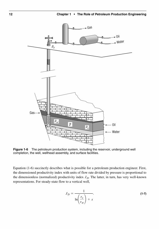
The reservoir, well, and surface facilities are sketched in Figure 1-6. The flow systemsfrom the reservoir to the entrance to the separation facility are the production engineering sys-tems that are the subjects of study in this book.
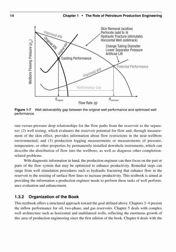
1.3 Well Productivity and Production Engineering1.3.1 The Objectives of Production EngineeringMany of the components of the petroleum production system can be considered together by graph-ing the inflow performance relationship (IPR) and the vertical flow performance (VFP). Both theIPR and the VFP relate the wellbore flowing pressure to the surface production rate. The IPR repre-sents what the reservoir can deliver, and the VFP represents what the well can deliver. Combined, asin Figure 1-7, the intersection of the IPR with the VFP yields the well deliverability, an expressionof what a well will actually produce for a given operating condition. The role of a petroleum produc-tion engineer is to maximize the well deliverability in a cost-effective manner. Understanding andmeasuring the variables that control these relationships (well diagnosis) becomes imperative.
While these concepts will be dealt with extensively in subsequent chapters, it is usefulhere to present the productivity index, J, of an oil well (analogous expressions can be written forgas and two-phase wells):
(1-6)J =q
p - pwf=
kh
arBmJD.
12 Chapter 1 • The Role of Petroleum Production Engineering
ptf
Oil
Gas
Water
pwfp
po
Oil
Gas
Water
Figure 1-6 The petroleum production system, including the reservoir, underground wellcompletion, the well, wellhead assembly, and surface facilities.
Equation (1-6) succinctly describes what is possible for a petroleum production engineer. First,the dimensioned productivity index with units of flow rate divided by pressure is proportional tothe dimensionless (normalized) productivity index The latter, in turn, has very well-knownrepresentations. For steady-state flow to a vertical well,
(1-7)JD =1
ln¢ re
rw≤ + s
.
JD.

1.3 Well Productivity and Production Engineering 13
For pseudosteady state flow,
(1-8)
and for transient flow,
(1-9)
where is the dimensionless pressure. The terms steady state, pseudosteady state, and tran-sient will be explained in Chapter 2. The concept of the dimensionless productivity index com-bines flow geometry and skin effects, and can be calculated for any well by measuring flow rateand pressure (reservoir and flowing bottomhole) and some other basic but important reservoirand fluid data.
For a specific reservoir with permeability k, thickness h, and with fluid formation vol-ume factor B and viscosity the only variable on the right-hand side of Equation (1-6) thatcan be engineered is the dimensionless productivity index. For example, the skin effect canbe reduced or eliminated through matrix stimulation if it is caused by damage or can be oth-erwise remedied if it is caused by mechanical means. A negative skin effect can be imposedif a successful hydraulic fracture is created. Thus, stimulation can improve the productivityindex. Finally, more favorable well geometry such as horizontal or complex wells can resultin much higher values of
In reservoirs with pressure drawdown-related problems (fines production, water or gasconing), increasing the productivity can allow lower drawdown with economically attractiveproduction rates, as can be easily surmised by Equation (1-6).
Increasing the drawdown by lowering is the other option available to theproduction engineer to increase well deliverability. While the IPR remains the same, reductionof the flowing bottomhole pressure would increase the pressure gradient and theflow rate, q, must increase accordingly. The VFP change in Figure 1-7 shows that the flowingbottomhole pressure may be lowered by minimizing the pressure losses between the bottomholeand the separation facility (by, for example, removing unnecessary restrictions, optimizing tub-ing size, etc.), or by implementing or improving artificial lift procedures. Improving well deliv-erability by optimizing the flow system from the bottomhole location to the surface productionfacility is a major role of the production engineer.
In summary, well performance evaluation and enhancement are the primary chargesof the production engineer. The production engineer has three major tools for well perform-ance evaluation: (1) the measurement of (or sometimes, simply the understanding of ) the
(p - pwf)
pwf(p - pwf)
JD.
m,
pD
JD =1
pD + s
JD =1
ln¢ re
rw≤ - 0.75 + s
,
14 Chapter 1 • The Role of Petroleum Production Engineering
rate-versus-pressure drop relationships for the flow paths from the reservoir to the separa-tor; (2) well testing, which evaluates the reservoir potential for flow and, through measure-ment of the skin effect, provides information about flow restrictions in the near-wellboreenvironmental; and (3) production logging measurements or measurements of pressure,temperature, or other properties by permanently installed downhole instruments, which candescribe the distribution of flow into the wellbore, as well as diagnose other completion-related problems.
With diagnostic information in hand, the production engineer can then focus on the part orparts of the flow system that may be optimized to enhance productivity. Remedial steps canrange from well stimulation procedures such as hydraulic fracturing that enhance flow in thereservoir to the resizing of surface flow lines to increase productivity. This textbook is aimed atproviding the information a production engineer needs to perform these tasks of well perform-ance evaluation and enhancement.
1.3.2 Organization of the BookThis textbook offers a structured approach toward the goal defined above. Chapters 2–4 presentthe inflow performance for oil, two-phase, and gas reservoirs. Chapter 5 deals with complexwell architecture such as horizontal and multilateral wells, reflecting the enormous growth ofthis area of production engineering since the first edition of the book. Chapter 6 deals with the
Flow Rate (q)
Skin Removal (acidize)Perforate (add to h)Hydraulic Fracture (stimulate)Horizontal Well (sidetrack)
Performance Gap
Potential Performance
Existing Performance
qoriginal qimproved
Improved IPROriginal IPR
Origi
nal V
FP
Improved VFP
Change Tubing DiameterLower Separator PressureArtificial Lift
Wel
lbor
e Fl
owin
g Pr
essu
re (p
wf)
Figure 1-7 Well deliverability gap between the original well performance and optimized wellperformance.

1.4 Units and Conversions 15
condition of the near-wellbore zone, such as damage, perforations, and gravel packing. Chapter7 covers the flow of fluids to the surface. Chapter 8 describes the surface flow system, flow inhorizontal pipes, and flow in horizontal wells. Combination of inflow performance and wellperformance versus time, taking into account single-well transient flow and material balance, isshown in Chapters 9 and 10. Therefore, Chapters 1–10 describe the workings of the reservoirand well systems.
Gas lift is outlined in Chapter 11, and mechanical lift in Chapter 12.For an appropriate product engineering remedy, it is essential that well and reservoir diag-
nosis be done.Chapter 13 presents the state-of-the-art in modern diagnosis that includes well testing,
production logging, and well monitoring with permanent downhole instruments.From the well diagnosis it can be concluded whether the well is in need of matrix stimula-
tion, hydraulic fracturing, artificial lift, combinations of the above, or none.Matrix stimulation for all major types of reservoirs is presented in Chapters 14, 15, and 16.
Hydraulic fracturing is discussed in Chapters 17 and 18.Chapter 19 is a new chapter dealing with advances in sand management.This textbook is designed for a two-semester, three-contact-hour-per-week sequence of
petroleum engineering courses, or a similar training exposure.To simplify the presentation of realistic examples, data for three characteristic reservoir
types—an undersaturated oil reservoir, a saturated oil reservoir, and a gas reservoir—are pre-sented in Appendixes. These data sets are used throughout the book. Examples and home-work follow a more modern format than those used in the first edition. Less emphasis isgiven to hand-done calculations, although we still think it is essential for the reader to under-stand the salient fundamentals. Instead, exercises require application of modern softwaresuch as Excel spreadsheets and the PPS software included with this book, and trends of solu-tions and parametric studies are preferred in addition to single calculations with a given setof variables.
1.4 Units and ConversionsWe have used “oilfield” units throughout the text, even though this system of units is inher-ently inconsistent. We chose this system because more petroleum engineers “think” inbbl/day and psi than in terms of and Pa. All equations presented include the constantor constants needed with oilfield units. To employ these equations with SI units, it will beeasiest to first convert the SI units to oilfield units, calculate the desired results in oilfieldunits, then convert the results to SI units. However, if an equation is to be used repeatedlywith the input known in SI units, it will be more convenient to convert the constant or con-stants in the equation of interest. Conversion factors between oilfield and SI units are givenin Table 1-1.
m3/s

16 Chapter 1 • The Role of Petroleum Production Engineering
Example 1-1 Conversion from Oilfield to SI UnitsThe steady-state, radial flow form of Darcy’s law in oilfield units is given in Chapter 2 as
(1-10)
for p in psi, q in STB/d, B in res bbl/STB, in cp, k in md, h in ft, and and in ft (s is dimen-sionless). Calculate the pressure drawdown in Pa for the following SI data, first byconverting units to oilfield units and converting the result to SI units, then by deriving the constantin this equation for SI units.
Data
SolutionUsing the first approach, we first convert all data to oilfield units. Using the conversion factors inTable 1-1,
re = 575 m, rw = 0.1 m, and s = 0.q = 0.001 m3/s, B = 1.1 res m3/ST m3, m = 2 * 10-3 Pa-s, k = 10-14 m2, h = 10 m,
(pe - pwf)rwrem
pe - pwf =141.2qBm
kh¢ ln
re
rw+ s≤
Table 1-1 Typical Units for Reservoir and Production Engineering Calculations
Variable Oilfield Unit SI Unit Conversion (Multiply SI Unit)
Area acre m2 2.475 * 10-4
Compressibility psi-1 Pa-1 6897
Length ft m 3.28
Permeability md m2 1.01 * 1015
Pressure psi Pa 1.45 * 10-4
Rate (oil) STB/d m3/s 5.434 * 105
Rate (gas) Mscf/d m3/s 3049
Viscosity cp Pa-s 1000
1.4 Units and Conversions 17
(1-11)
(1-12)
(1-13)
(1-14)
(1-15)
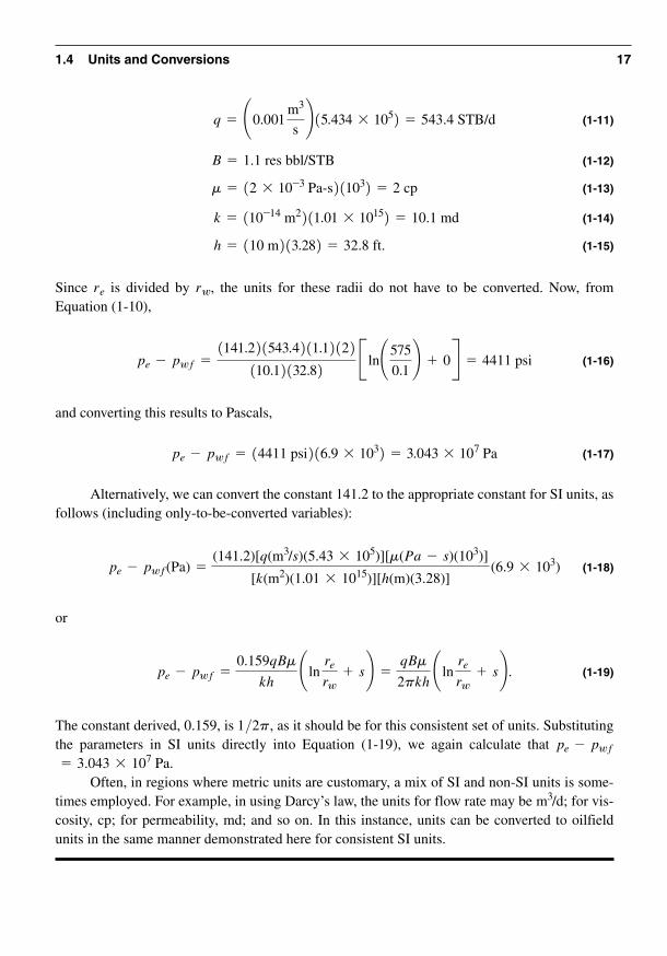
Since is divided by the units for these radii do not have to be converted. Now, fromEquation (1-10),
(1-16)
and converting this results to Pascals,
(1-17)
Alternatively, we can convert the constant 141.2 to the appropriate constant for SI units, asfollows (including only-to-be-converted variables):
(1-18)
or
(1-19)
The constant derived, 0.159, is as it should be for this consistent set of units. Substitutingthe parameters in SI units directly into Equation (1-19), we again calculate that
Often, in regions where metric units are customary, a mix of SI and non-SI units is some-times employed. For example, in using Darcy’s law, the units for flow rate may be for vis-cosity, cp; for permeability, md; and so on. In this instance, units can be converted to oilfieldunits in the same manner demonstrated here for consistent SI units.
m3/d;
= 3.043 * 107 Pa.pe - pwf
1/2p,
pe - pwf =0.159qBm
kh¢ ln
re
rw+ s≤ =
qBm
2pkh¢ ln
re
rw+ s≤ .
pe - pwf(Pa) =(141.2)[q(m3/s)(5.43 * 105)][m(Pa - s)(103)]
[k(m2)(1.01 * 1015)][h(m)(3.28)](6.9 * 103)
pe - pwf = (4411 psi)(6.9 * 103) = 3.043 * 107 Pa
pe - pwf =(141.2)(543.4)(1.1)(2)
(10.1)(32.8)B ln¢ 575
0.1≤ + 0R = 4411 psi
rw,re
h = (10 m)(3.28) = 32.8 ft.
k = (10-14 m2)(1.01 * 1015) = 10.1 md
m = (2 * 10-3 Pa-s)(103) = 2 cp
B = 1.1 res bbl/STB
q = ¢0.001m3
s≤(5.434 * 105) = 543.4 STB/d
References1. Amyx, J.W., Bass, D.M., Jr., and Whiting, R.L., Petroleum Reservoir Engineering,
McGraw-Hill, New York, 1960.
2. Craft, B.C., and Hawkins, M. (revised by Terry, R.E.), Applied Petroleum Engineering,2nd ed., Prentice Hall, Englewood Cliffs, NJ, 1991.
3. Dake, L.P., Fundamentals of Reservoir Engineering, Elsevier, Amsterdam, 1978.
4. Darcy, H., Les Fontaines Publiques de la Ville de Dijon, Victor Dalmont, Paris, 1856.
5. Earlougher, R.C., Jr., Advances in Well Test Analysis, SPE Monograph, Vol. 5, SPE,Richardson, TX, 1977.
6. Muskat, M., Physical Principles of Oil Production, McGraw-Hill, New York, 1949.
18 Chapter 1 • The Role of Petroleum Production Engineering

711
Index
A
ACA (after-closure analysis), 430, 433, 434–35Acid
acid/rock interactions (See Matrix acidizing)additives, in sandstone acidizing
design, 512concentration profiles, 475fgas, 68injection into gas reservoir, 494–96placement, mechanical, 496–97reaction products, precipitation of, 461–64response curves, 471fselection, in sandstone acidizing design,
470–71, 471ttransport to mineral surface, 460–61
Acid capacity numberfast-reacting minerals, 474, 477HCI, 510slow-reacting minerals, 474
Acid fracture conductivity, 545–52average, 551, 552teffective, 548–49tfracture width profile along a fracture, 546f
Acid fracturing, 541–54acid diffusion coefficients, 544facid fracture conductivity, 545–52acid-fractured well, productivity of, 552–53,
553facid penetration distance, 544–45acid penetration in fractures, 542–45, 543fvs. matrix acidizing, 443propped fracture vs. acid fracture performance,
553–54well productivity, 552–53, 553f
Acidizing process, optimal rate schedule formonitoring, 486–96
acid injection into gas reservoir, 494–96acid treatment data, 492tdesign chart for monitoring acidizing,
Paccaloni’s, 489–90, 490f
injection rate and pressure, maximum, 487–89,488f
maximum p, maximum rate procedure,Paccaloni’s, 489–90, 490f
skin factor evolution during acidizing, 486f,490–93, 493t, 494f
Acidizing treatment. See also Matrix acidizingin sandstone acidizing design, 512–13
Acid-mineral reaction kinetics, 453–60constants in HCI-mineral reaction kinetics
models, 455tconstants in HF-mineral reaction kinetics
models, 456tdissolution rate of rotating disk of feldspar,
457–58fluosilicic acid with sandstone minerals, 460HCl and weak acids with carbonates, 454–55HF with sandstone minerals, 455–60measurement of, 454relative reaction rates of sandstone minerals,
459Acid-mineral reaction stoichiometry, 446–52
chemical reactions, primary, 448tdissolving power of acids, 450t, 451tHCI preflush volume, calculating, 452spending of acid components, 451t
Acid penetrationdistance, 544–45in fractures, 542–45, 543f
Acid volume, 472–96acidizing process, optimal rate schedule for
monitoring, 486–96design, 478–80injection rate and, 472–96to remove drilling mud damage, 480–81, 481fsandstone acidizing models, 472–85treatment design, competing factors
influencing, 472After-closure analysis (ACA), 430, 433, 434–35Agarwal-Gardner type curves, 578–79, 578fAltered permeability, 8
¢
Note: Page numbers with “f” indicate figures; those with “t” indicate tables.

712 Index
Altered porosity, 8Anisotropy, 2, 3f, 401
dependence of deviated well skin factor onreservoir, 134
horizontal, 113ratio, 98, 104vertical-to-horizontal, 95, 97–98, 112
Annular flow, 179, 188, 220, 221, 221f, 222,223f, 224f, 226
Annular mist flow, 222, 223f, 224f, 226Areal extent, 7–8Arps decline curve analysis, 388, 388t, 390Artificial lift, 11, 13
B
Babu-Odeh model, 103–9schematic of, 103fwell performance with, 106–8
Backflow, 392Baker flow regime map, 222f, 225–26Ball sealers, 497Barnett shale formation, 586Beam loads, sucker rod and, 345–47Beam pumping units, 345Bean (choke diameter), 241Before-closure behavior, 430, 432, 433, 435–37Beggs-Brill correlation, 201–6, 223, 226–28Beggs-Brill flow regime map, 224f, 225, 226B factor correlations, 693tBilinear flow, 416, 416f, 418–20Biological damage, 157Biwing fracture, events with, 648fBorate-crosslinked fluid, properties of, 638–39f,
638–40Bottomhole flowing pressure, 1, 4, 6, 10–11, 13
in gas well, calculating, 182–84in gas well, flow rate vs., 78–79, 78t, 79fwith GLR values of 300 and 800 SCF/STB,
264–65injected gas, 313injection rate increase, impact of, 312–13modified Hagedorn-Brown correlation, 266,
266tproduction rates, 266, 266treduction in, VFP curve and, 268well deliverability, 261wellhead pressure, 262
Bottomwater, excessive, 380–81Boundaries, 2, 3f
Boundary dominated flow, 577Breakdown pressure, 602, 604, 605, 605f, 606fBrill-Mukherjee model, 192Bubble flow, 188, 210
dispersed, 222, 222f, 223f, 224f, 226elongated, 222, 222f, 223f, 224fGriffith correlation, 198–201
Bubble-point pressure, 6introduction, 41–42PVT properties below, 43, 45fsaturated oil characterized by, 42–43
Buijse-Glasbergen model, 529–31, 531fBuildup analysis. See also Log-log diagnostic plot
limited-entry vertical well, 413–14, 414ffor limited-entry well, 413–14, 414fmodel match for, 409f, 414f
C
Cake resistance, effect on acid placement, 506–8injection rate history, total, 508finjection rate into high-permeability layer,
507finjection rate into low-permeability layer, 507f
Carbonate acidizing design, 519–55acid fracturing, 541–54HCl acid and weak acid reactions with,
454–55horizontal wells, acidizing of, 554–55, 554fintroduction, 519–22matrix acidizing design for carbonates, 535–41skin evolution during, 539–40, 540fwormhole formation and growth, 522–25wormhole propagation models, 525–35
Cased hole logs, 368–87. See also Production logevaluation
Cased well, 9–10, 10fcompletion skin factors, 138–46
Cavity completion, 677Cemented well, 9–10, 10fCement evaluation, 368–69, 369fCement squeeze, 370, 374–75Channeling, 374–375f, 374–76, 376fChemical precipitation, 154–55Chen equation, 177–78, 197, 206Choke, 236–47
critical flow, 242, 246, 247diameter (bean), 241flow coefficient, 240fflow rate, 237

gas-liquid flow, 243–47horizontal well flow profile, 255fkinetic energy pressure drop through, 240performance curves, 246–47, 247fschematic of, 237fsingle-phase gas flow, 241–43single-phase liquid flow, 240–41size, 242, 243f, 244–46, 255ftransverse hydraulic fractures, 592–94
Churn flow, 188, 191Closure stress, 430–37
after-closure analysis, 430, 433, 434–35before-closure behavior, 430, 432, 433,
435–37vs. proppant conductivity, 643, 644f
Colebrook-White equation, 176–77Completion damage, 159–61Completion failure avoidance, 698–99Complex fracture geometry, creating, 615–16Complex fracturing, defined, 610, 615Compressible, single-phase flow of, 179–84
calculation of bottomhole flowing pressure ingas well, 182–84
equation for pressure drop, 179–82Condensate, 7Conductive fracture length, 562–66, 565fConductivity performance
finite fracture, 578–79infinite fracture, 574–78
Conical wormhole forms, 523Connate water saturation, 4Continuous gas-lift design, 303–10
gas compressors, power requirements for,309–10
GLR and gas-lift rate, calculating, 303–4natural vs. artificial flowing gradient, 303–4point of injected gas, 305–8pressure of injected gas, 304–5tubing performance curve, 306, 308f
Continuous gas-lift system, 300–301, 301fCorrelations
Beggs-Brill, 201–6, 223, 226–28factor, 693t
Dukler, 231–34Eaton, 228–31empirical constants in two-phase critical flow,
243–44, 244tflow in formation in non-Darcy coefficient,
81–82tGilbert, 243, 244–46, 244tGray, 206–10
Griffith, 198–201Hagedorn-Brown, 192–98, 228Omana, 244, 245, 246porosity vs. permeability, 8pressure gradient, 226, 230, 231, 232property, for two-phase systems, 47–52Ros, 243, 244–46, 244ttwo-phase, for horizontal well inflow, 115–16
Cricondentherm, 7Critical depth for horizontal fracture, 607–8, 608fCritical flow
vs. critical point of fluid, 237empirical correlations for, in gas-liquid flow,
243–44, 244tthrough choke, 242, 246, 247
Critical point, 6Crossover method of gravel pack placement, 680,
681fCylindrical flow, 401, 418
D
Damkohler number, 474–75Darcy. See also Non-Darcy flow
experiment, 8–9, 9flaw in radial coordinates, 19
Data farcs, 303Decline curve analysis, 387–90, 590, 591f
in kinetic energy pressure drop, meaning of,234
pF, frictional pressure drop, 176–79pKE, pressure drop due to kinetic energy
change, 174–76pPE, pressure drop due to potential energy
change, 173–74Depth
critical, for horizontal fracture, 607–8, 608fstresses vs., 604
Design fracture treatment to achieve optimaldimensions, 634–35
Deterministic models, 192Deviated production wells in HPF, 694–97,
698fDew-point curve, 7Diagnostic fracture injection test (DFIT).
See Fracture calibration injection falloff
Differential depletion, 392, 393Dimensionless effective wellbore radius, 563,
564, 564f
¢
¢¢
¢
b
Index 713

Dimensionless groups in sandstone acidizingmodel, 476t
Dimensionless productivity index, 13Discontinuities, 2, 3fDispersed bubble flow, 222, 222f, 223f, 224f, 226Distributed flow, 220–26
bubble, 221f, 222, 222f, 223f, 224f, 226mist, 221f, 222, 222f
Downhole instruments, 14Downhole properties, estimating, 51–52Draining patterns, irregular, 30–34
production rate and, 30, 32reservoir pressure in adjoining drainage areas,
determining, 32–34, 32fshape factor for closed, single-well drainage
areas, 31fDrawdown, 13, 16, 22Drawdown failure condition, 666–67, 671fDrilling damage
mud, acid volume needed to remove, 480–81,481f
sources of, 157–59Dual-porosity approach, 592Dukler correlation, 231–34, 233fDuns-Ros flow regime map, 188, 190fDynamic displacement pumps, 335, 354–59
electrical submersible, 354–59Dynamic value, 610Dynamometer card
for elastic rods, 348ffrom properly working rod pump, 348frod pump performance analyzed from, 347–50shapes, 348–50, 349f
E
Eaton correlation, 228–31friction factor, 228, 229fholdup, 228, 229f
Economides et al. model, 109–13parallelepiped model with appropriate
coordinates, 110fresults summary, 113tshape factors, approximate, 111twell performance with, 112–13
Effective drainage radius, 80, 390, 418Effective wellbore radius, 21–22Electrical resistivity, 5–6, 5fElectrical submersible pump (ESP), 335, 354–59
completion, 353f, 354, 355f
design, 357, 358–59pump characteristic chart, 354, 356f, 358fselecting, 356–57
Ellipsoidal flow around perforation, 476fElongated bubble flow, 222, 222f, 223f, 224fEmpirical models, 192Emulsions, fluid damage and, 155–56Equations
Chen, 177–78, 197, 206Colebrook-White, 176–77flow regimes, 402–3tHagen-Poiseuille, 171, 172mechanical energy balance, 172, 179, 192,
193–94, 335pressure drawdown, 25pressure drop, 179–82
ESP. See Electrical submersible pump (ESP)EUR (expected ultimate recovery), 388–90, 389fExpected ultimate recovery (EUR), 388–90, 389fExponential decline, 577
F
Fanning friction factor, 176, 197, 210Feldspar, dissolution rate of rotating disk of,
457–58Fetkovich’s approximation, 57–58F-function constants, 573, 573tFine migration, mechanisms for, 154Fines, 151Finite fracture conductivity performance, 578–79Fittings, equivalent lengths of, 238–39tFlow, 217–56
capacity of low-pressure gas line, 219–20horizontal pipes, 217–36horizontal wellbores, 250–56introduction, 217surface gathering systems, 247–50through chokes, 236–47
Flow geometries. See Flow regimesFlow profile used to evaluate damaged well, 372Flow regime analysis, 400–437
flow regime equations, 402–3tfracture calibration injection falloff, 429–37,
430, 431fhorizontal well, 429, 429flimited-entry vertical well, 410–16, 410fpermeability, determining, 401pressure buildup analysis, 406–7, 410fradial flow geometries for vertical wells, 405
714 Index

reservoir pressure, estimating, 405–6skin factor, estimating, 405transient well analysis, 400–437unit conversion factors, 404tvertically fractured vertical well, 416–28wellbore storage, 407–10
Flow regime maps, 188, 190–91Baker, 222f, 225–26Beggs-Brill, 224f, 225, 226Duns-Ros, 188, 190fMandhane, 223, 223f, 225, 226Taitel-Dukler, 190–91, 190f, 223, 224f
Flow regimes. See also Single-phase flowregimes; Two-phase flow regimes
defined, 400–401distributed, 220, 221f, 222, 223, 224fequations, 402–3tintermittent, 220, 221f, 222, 223, 224f, 226,
227limited-entry vertical well, 410–11, 410fmaps of (See Flow regime maps)pressure buildup analysis, 406–7, 410fsegregated, 220–21, 221f, 223, 224fvertically fractured vertical well, 416–19, 416f
Fluid damage, 155–56Fluid diversion in carbonates, 540–41Fluid efficiency in fracture calibration injection
falloff, 430, 432, 433t, 435Fluid placement and diversion, 496–509
ball sealers, 497mechanical acid placement, 496–97particulate diverting agents, 497–508viscous diversion, 508–9
Fluid saturations, 4–6Fluid volume
calculations, total, 626–28requirements, 624–29
Fluosilicic acid reactions with sandstone minerals,460
Formation damage, 157–63completion damage, 159–61drilling damage, 157–59injection damage, 162–63production damage, 161–62during well operations, sources of, 157–63
Formation damage mechanisms, 151–57biological damage, 157chemical precipitation, 154–55emulsions, 155–56fine migration, mechanisms for, 154mechanical damage, 156
particle plugging of pore spaces, 151–54permeability, 155–56wettability changes, 155–56
Formation flow velocityin gravel pack completion, 687–88to HPF, 693–94
Formation fluid sampling, 391–93Formation linear flow, 416Formation linear flow approximation,
577–78Formation sand production, factors affecting,
662–72drawdown failure condition, 666–67, 671fevents to induce sand problems, 663fMohr circle, 663, 663fMohr-Coulomb criterion, 664–65, 664f, 666fnumerical simulation cases, conditions for,
667–69, 668t, 669fproductivity ratio vs. perforation
density, 672fshut-in, 669–70simulated failure criteria, 670f
Frac-pack completion, 688–93factor correlations for, 693t
flowing perforations, number of, 692model for radial and fracture-face damage,
689–90, 690fskin, 690–91
Fracture calibration injection falloff, 429–37, 430,431f
closure stress, 430–37fluid efficiency, 430, 432, 433t, 435fracture height, 432, 433t, 436fracture models, 432, 433t, 434fracture width, 432, 433t, 436g-function, 430leakoff coefficient, 430, 432, 433t, 435log-log diagnostic plot, 430, 431fparameters, 430power law fracture surface growth assumption,
430, 432sequence of events observed in, 430, 431f
Fracture diagnostics, 646–50fracture geometry measurement, 647–50fracturing pressure analysis, 646–47Nolte-Smith analysis pressure response modes,
647tNolte-Smith plot, 646–47, 647f
Fracture direction in reservoir rock, 606–7, 608–9
Fractured oil well model match, 422f
b
Index 715

Fractured well behavior in low-permeabilityreservoirs, 574–79
Agarwal-Gardner type curves, 578–79, 578ffinite fracture conductivity performance,
578–79formation linear flow approximation,
577–78infinite fracture conductivity performance,
574–78long-term, 575–76, 577f
Fractured well performance, 585–92shale reservoirs, 586–92tight gas reservoirs, 586
Fractured well productivity, 566–73Fracture geometry, 609–16. See also Fracture
widthcomplex, creating, 615–16evolving, 628–29, 629fmeasurement, 647–50TSO treatments, 615
Fracture geometry and net pressure, 616–35
design fracture treatment to achieve optimaldimensions, 634–35
fluid volume calculations, total, 626–28fluid volume requirements, 624–29height migration, 621–23, 622f, 624fnet fracturing pressure, 616–20, 621pad volume calculations, total, 626–28proppant schedule, 629–30, 631fpropped fracture width, 631–35
Fracture geometry for maximizing fractured well productivity, 566–73, 568f, 569f, 570f
calculating, 571–72F-function constants, 573, 573tunified fracture design, 567–73
Fracture geometry measurement, 647–50microseismic monitoring, 648–50tiltmeter mapping, 650tracers and temperature, 650
Fracture heightfracture calibration injection falloff, 432, 433t,
436mapping, with microseismic monitoring,
650fmeasured with radioactively tagged proppant,
382–83, 384fmigration, 621–23, 622f, 624fproduction log evaluation, measurement of,
381
temperature log interpretation of, in production log evaluation, 382, 383f
Fracture initiation pressure, calculating, 606Fracture injection tests, 603Fracture length, 562–66, 565fFracture models
KGD, 432, 433tPKN, 433t, 434radial, 432, 433t
Fracture patterns, 586–89, 588f, 589fdrainage, 589fmicroseismic map of, 589fin tight reservoirs, 586, 588, 588f
Fracture ports, 653Fracture properties in HPF, 697tFractures. See Acid fracturingFracture width
fracture calibration injection falloff, 432, 433t,436
KGD model, 609–10, 614, 614fnon-Newtonian fluid, 610, 613PKN model, 609, 610–13, 611fradial model, 609, 615
Fracturing. See Acid fracturing; Hydraulicfracturing for well stimulation
Fracturing fluids, 635–42frictional pressure drop during pumping,
641–42perfect, 646rheological properties, 636–41selection guide, 637fusage, 635f
Fracturing horizontal wells, 651–55fracture orientation in, 651–52, 651fwell completions for multiple fracturing,
652Fracturing pressure analysis, 646–47Frictional pressure drop
pF, 176–79during pumping, 641–42well length, 11
Friction factor correlation, Eaton, 228, 229f
Froth flow, 222, 223f, 224f, 226Froude number, 223, 224f, 226Full-strength mud acid, 470Furui et al. model, 100–103
schematic of, 101fwell performance with, 102–3wormhole, 531–35, 534f
¢
716 Index

G
Gaseffect on pump efficiency, 350–52, 350fin reservoir fluid, 11use of term, 4
Gas anchors, 352Gas compressibility factor
calculated, in transient IPR for gas well, 88–90tcorrection for nonhydrocarbon gases, 68–71for mixtures of hydrocarbon gases, 63–65, 64fof sour gas, 70–71, 70t
Gas compressors, power requirements for, 309–10Gas coning, 379–80, 380fGas deviation factor. See Gas compressibility
factorGas flow, 218–20, 241–43. See also Gas-liquid
flowcapacity of low-pressure gas line, 219–20excessive, 374, 378–79, 378f, 379fkinetic energy pressure drop in, 218performance for different choke sizes, 242, 243fpreferential, 376–77single-phase, 218–20, 241–43
Gas formation volume factor, 7–8, 74–75Gas gravity, 61–63
pseudocritical properties from, 66–68Gas isothermal compressibility, 75–76Gas lift, 11, 299–332
depleting reservoir, 330, 330feconomics of, 324–26, 325f, 325tintroduction, 299near-wellbore damage and, 232f, 321, 322–24onset of, 331–32performance, GLR and, 261–62purpose of, 261requirements vs. time, 328–32tubing size vs. gas-lift requirements, 326–27,
327f, 328f, 329ftypes of, 300–301, 301fvalves, unloading wells with multiple, 310–12
Gas-lift designcontinuous, 303–12optimization of, 312–16
Gas-lift design, continuous, 303–12flowing gradient, natural vs. artificial, 303–4gas compressors, power requirements of,
309–10Gas-lift design, optimization of, 312–16
GLR values, 312–15, 315f, 316f, 318f, 319finjection rate increase, impact of, 312–13
maximum production rate with gas lift,314–16, 315f, 316f
sustaining production rate while pressuredepletes, 313–14
Gas-lift performance curve, 316–28, 321fdevelopment of, 319–20IPR and optimum gas lift, 321ftime dependency, 320f
Gas-lift system, 299–302. See also Gas-liftvalves
completions of, 299, 300, 301fschematic of, 300f
Gas-lift valves, 300–301, 302fmultiple, unloading wells with, 310–12, 311fopening and closing, 301positioning, 300pressure regulator, 301, 302f
Gas-liquid flow, 243–47choke size for, 244–46horizontal, predicting, 225–26through chokes, 243–47
Gas-liquid ratio (GLR)continuous gas-lift design, 303–4gas lift performance, 261–62gradient curves for, 303gradient curves for range of values, 265fliquid production rate vs., 319f, 320fmaximum gas-lift production rate, 312–15,
315f, 316f, 318foptimum gas-lift performance, 317–21,
317fVFP and, impact on, 264–65
Gas production gathering systems. See Surfacegathering systems
Gas viscosity, 71–74, 72–73fGas well
acid injection into, 494–96horizontal, inflow performance relationship
for, 114–15material balance, 294–96performance and production forecast, 294–96,
296ttransient flow of, 84–91
Gas well deliverability, 270–73, 272fapproximation of, 76–79curve, formation of, 82–83, 84fflow rate vs. bottomhole pressure for gas well,
78–79, 78t, 79fIPR and VFP in, 270–73, 272ffor non-Darcy flow, 79–84, 84ftubing size and, 272–73, 273f
Index 717

Gel frac vs.Waterfrac map, comparison of, 649fGeneralized expression, 281–82G-function, 430Gilbert correlation, 243, 244–46, 244tGLR. See Gas-liquid ratio (GLR)Gradient curves, 213, 213f
expanded-scale, 332fin gas-lift requirements vs. time, 329ffor GLR, 265f, 303intersection of gas injection pressure with,
309f, 310in tubing size vs. gas-lift requirements,
326–27, 327f, 328fGravel pack completion, 678–88
factor correlations for, 693tformation flow velocity, 687–88gravel and screen sizing, 682–86, 683–84tgravel pack evaluation, 688high-rate water pack, 686–88log showing response to voids in gravel pack,
689fproductivity of gravel-packed wells, 686skin factors, 148–51types, 678, 679f
Gravel packing, 10, 10fGravel pack placement, 678–80
crossover method of, 680, 681ffor inside-casing gravel packs, 680, 681fin open-hole or underreamed casing
completions, 679, 680fGravel sizing, 682–86, 683–84tGray correlation, 206–10Griffith correlation, 198–201Gross height, 4
H
Hagedorn-Brown correlation, 228modified (mH-B), 192–93, 266, 266toriginal, 193–98
Hagen-Poiseuille equation for laminar flow inpipe, 171, 172
Halo, 688Hawkins’ formula, 122–26HCI. See Hydrochloric (HCl) acidHeight. See Fracture heightHeight migration, 621–23, 622f, 624fHeterogeneities, 2, 3f. See also Acid-mineral
reaction kinetics
HF. See Hydrofluoric (HF) acidHigh-conductivity vertically fractured vertical
well, production data analysis for, 420–24,423f
High-performance fracturing (HPF), 693–97in deviated production wells, 694–97, 698fflow directly to abandoned perforations,
696fformation flow velocity to, 693–94perforating strategy for, 697–98reservoir and fracture properties, 697t
High-permeability layersexcessive flow through, 378–79, 378f, 379fpreferential flow through, 376–77
High-permeability reservoirs, 560fHigh-rate horizontal well, pressure drop in,
252–54High-rate water pack, 686–88Holdup behavior, 185–87Holdup phenomenon, 185–87Horizontal anisotropy, 113Horizontal borehole, measurements along, 393,
393fHorizontal gas wells, inflow performance
relationship for, 114–15Horizontal permeability, 401Horizontal pipes, flow in, 217–36
Beggs-Brill correlation, 226–28Dukler correlation, 231–34Eaton correlation, 228–31flow regimes, 220–26, 221fgas, single-phase flow, 218–20liquid, single-phase flow, 217–18pressure gradient correlations, 226pressure traverse, calculating, 234–36two-phase flow, 220–36wellbore pressure drop for, 252–56
Horizontal wellacidizing, 554–55, 554fdamage skin effect, 134–37drainage pattern formed around, 96fgas, inflow performance relationship for,
114–15inflow, two-phase correlations for, 115–16introduction, 95–97multilateral well technology, 116–17, 117fperforation skin factor for, 145–46production from, 95–117productivity index for, vs. vertical wells,
108–9
b
718 Index

pseudosteady state flow, 103–13steady-state well performance, 97–103
Horizontal wellbores, flow in, 250–56. See alsoPressure drop
HPF. See High-performance fracturing (HPF)Hydraulic fracture, 9
defined, 559diagram of, 560ftubing size selection in gas well, 272–73
Hydraulic fracturing for well stimulation, 559–94
choke effect for transverse hydraulic fractures,592–94
conductive fracture length, 562–66, 565feffective wellbore radius, 564ffractured well behavior, 574–79fractured well performance, 585–92fracture geometry for maximizing fractured
well productivity, 566–73, 568f, 569f, 570ffracture length, 562–66, 565ffracture patterns, 586–89, 588f, 589fhigh-permeability reservoirs, production and
recovery acceleration, 560fintroduction, 559–62low-permeability reservoirs, 561f, 574–79non-Darcy flow, 579–85shale reservoirs, fractured well performance
for, 586–92skin effect, 562–66, 565fSRV, 562f, 588tight gas reservoirs, fractured well
performance for, 586, 588fHydraulic fracturing treatments, design and
execution of, 601–55fracture diagnostics, 646–50fracture geometry, 609–16fracture geometry and net pressure, created,
616–35fracturing fluids, 635–42fracturing horizontal wells, 651–55introduction, 601–2proppants and fracture conductivity, 642–46proppant schedule, 629–30, 631freservoir rock, fracturing of, 602–9
Hydrocarbon mixture, schematic phase diagramof, 42f
Hydrocarbons, 4Hydrocarbon saturation, 5Hydrochloric (HCl) acid
acid capacity number for, 510
constants in HCI-mineral reaction kineticsmodels, 455t
effective diffusion coefficient of, 460, 461fpreflush, 509–11preflush volume, calculating, 452weak acid reactions with carbonates, 454–55
Hydrofluoric (HF) acidconstants in HF-mineral reaction kinetics
models, 456tdissolving power of, 451treactions with sandstone minerals, 455–60
Hydrostatic pressure, 10–11
I
Inclined wells, skin components for, 126–27Incompressible, single-phase flow of, 168–79
annular flow, 179laminar or turbulent flow, 168–69pressure-drop calculations, 172–79velocity profiles, 169–72
Infinite-acting behavior, transition topseudosteady state from, 29
Infinite-acting radial flow, 564, 566Infinite-acting reservoir
IPR calculations, 275–77prediction of production rate in, 25–26rate decline for, 26f
Infinite fracture conductivity performance, 574–78Inflow performance for two-phase reservoir,
55–56Inflow performance relationship (IPR), 11, 13,
14f, 34–37. See also IPR curvechanges in, 267–68, 268fgas reservoirs, 270–73, 272fhorizontal gas wells, 114–15pseudosteady-state, influence of average
reservoir pressure, 35, 37, 37fskin effect on, 267, 267fsteady-state, influence of skin effect, 35, 36ftransient, 34–35, 36f, 87–91transient production rate forecast, 275–77of two-phase reservoirs, 268–70, 269fVFP and, combination of, 262–68
Initial reservoir pressure, 275Injected gas
bottomhole pressure, 313point of, 305–8pressure of, 304–5
Index 719

Injection damage, 162–63Injection rate, 472–96. See also Acid volumeInjection well diagnosis, 383, 384–85Inside-casing gravel pack, 678, 679f, 680, 681fIn-situ average density, 194, 200, 201, 205, 207,
209In-situ average liquid velocity, 198In-situ stresses, 602–3Integral of RNP (IRNP)
computing, 398, 399fvertically fractured vertical well, diagnostic
plot, 424fIntermittent flow, 220–27
plug, 221f, 222slug, 220, 221f, 222, 222f, 223f, 224f, 226
Intermittent gas lift, 300–301, 301fInterstitial water saturation, 4Inverse injectivity, 491IPR curve, 262, 263f. See Inflow performance
relationship (IPR)with declining reservoir pressure, 330fat different reservoir pressures, 331fin gas well deliverability, 271–73, 272f, 273ffor oil well under pseudosteady-state
conditions, 279foptimum gas-lift performance, 317–21, 317f,
321ffor solution gas-drive reservoir, 292ffor steady-state flow, 275transient, 275–77, 276ffor two wellhead flowing pressures in
two-phase reservoir, 270fIsothermal compressibility, 75–76, 277Isotropy, 112
J
Joshi model, 97–100schematic of, 97fwell performance with, 99–100, 100f
K
KGD fracture model, 432, 433twith fracture width, 609–10, 614, 614f
Kinetic energy pressure drop, 217–19computing, 228, 230
in, meaning of, 234differential form of, 218–19
due to change, 174–76neglecting, 228, 230, 235pressure gradient correlations, 226, 230, 231,
232in single-phase gas flow, 218in single-phase liquid flow, 217through choke, 240
Kinetics of a reaction, 453. See also Acid-mineralreaction kinetics
L
Laminar or turbulent flow, 168–69Leakoff coefficient, 430, 432, 433t, 435Lean gas reservoirs, 7Limited-entry geometry, 411Limited-entry vertical well, 410–12
buildup analysis for, 413–14, 414fflow regimes for, 410–11, 410flog-log diagnostic plot, 412ftest design, 415–16, 415f
Liquid density, 48–49, 49fLiquid flow. See also Gas-liquid flow
kinetic energy pressure drop in, 217pressure drop in water injection supply line,
218single-phase, 217–18, 240–41
Liquid holdup, 192Beggs-Brill correlation, 226–28Dukler correlation, 231–34, 233fEaton correlation, 228–31, 229f
Liquids in gas wells, lifting, 359–61. See alsoPlunger lift
Logging while drilling (LWD), 2Log-log diagnostic plot
fracture calibration injection falloff, 430, 431flimited-entry vertical well, 412fwell rate and pressure transient analysis,
395–96, 395fLongitudinal fractures, 651, 651fLow-conductivity vertically fractured vertical well
buildup analysis for, 425–26production data analysis for, 426–28, 428f,
428tLow-permeability reservoirs
fractured well behavior in, 574–79production and reserves enhancement from,
561fLow-pressure gas line, flow capacity of, 219–20Low productivity, 372
¢
720 Index

M
Mandhane flow regime map, 223, 223f, 225, 226Maps/mapping
fracture height, 650fGel frac vs.Waterfrac, comparison of, 649fwith microseismic monitoring, 650fof multi-stage fracture treatment, 649ftiltmeter, 650
Matrix acidizing, 443–64vs. acid fracturing, 443acid-mineral reaction kinetics, 453–60acid-mineral reaction stoichiometry, 446–52acid transport to mineral surface, 460–61chemical reactions, primary, 448tin damaged and undamaged wells, benefits of,
444–46, 445–46fdissolving power of acids, 450tdissolving power of HF acid, 451tHCI preflush volume, calculating, 452introduction, 443–46molecular weights of species in, 449tprecipitation of acid reaction products,
461–64spending of acid components, 451t
Matrix acidizing design for carbonates, 535–41acid selection design chart, 537facid type and concentration, 535–36acid use guidelines, 536tacid volume and injection rate, 536–38fluid diversion in carbonates, 540–41monitoring the acidizing process, 538–40viscoelastic surfactant, 540–41, 541f
Matrix stimulationcorrelations of porosity vs. permeability and, 8near-wellbore permeability recovered or
improved by, 9skin effect reduced or eliminated through, 13
Measurementsacid-mineral reaction kinetics, 454along horizontal borehole, 393, 393felectrical resistivity formation, 5–6fracture geometry, 647–50fracture height with radioactively tagged
proppant, 382–83, 384fpetroleum thermodynamic properties, 7porosity, 3–4pressure, 14production logging, 14rate-vs.-pressure drop relationships, 14reaction kinetics, 454
well testing, 2, 14wireline formation test, 392f, 393, 393f
Measurements while drilling (MWD), 2Mechanical acid placement, 496–97Mechanical damage, 156Mechanical energy balance equation, 172, 179,
192, 193–94, 335MH-B (modified Hagedorn-Brown method),
192–93Microseismic monitoring, 648–50
biwing fracture, events with, 648fmap comparison of Gel frac vs.Waterfrac, 649fmap of multi-stage fracture treatment, 649fmapping fracture height with, 650f
Minifracs, 303. See also Fracture calibrationinjection falloff
Mist flowannular, 222, 223f, 224f, 226distributed, 221f, 222, 222f
Mobility, 9Model match
buildup analysis, 409f, 414ffractured oil well, 422fparameters, 423t, 428t
Modified Hagedorn-Brown method (mH-B), 192–93Mohr circle
in drawdown failure condition, 666–67, 667fin formation sand production, 663, 663fMohr-Coulomb criterion, 664–65, 664f, 666f
Moody friction factor chart, 176, 178fMultilateral well technology, 116–17, 117fMultiphase flow in wells, 184–213
holdup behavior, 185–87pressure traverse calculations, 210–13two-phase flow regimes, 187–91two-phase pressure gradient models, 191–210
Multiple fracturing, well completions for, 652openhole fracturing, 652open hole with liners and sleeves for, 652–53,
653–54fperf and plug fracturing, 655
Multi-stage fracture treatment, map of, 649f
N
NAc,F and NDa,S, determining from data, 477–78, 478f
Natural gascorrelations and calculations for, 66–76gas formation volume factor, 74–75
Index 721

Natural gas (continued )gas gravity, pseudocritical properties from,
66–68gas isothermal compressibility, 75–76gas viscosity, 71–74, 72–73fgravity of, 62–63molecular weights and critical properties for,
62tnonhydrocarbon gases, 68–71
Natural gas reservoirsgas gravity, 61–63gas well deliverability, 76–84gas well transient flow of, 84–91introduction, 61–66production from, 61–91real gas law, 63–66
Naturally flowing well, 11Near-well
damage and perforations, 145radial flow, 9
Near-wellborecondition and damage characterization (See
Skin effects)permeability, 9region, 20treatment (See Matrix acidizing)zones, 10, 10f
Net fracturing pressure, 616–20, 621Net height, 4Newtonian fluid
non-, with fracture width, 613single-phase flow of compressible, 179–84single-phase flow of incompressible, 168–79
No-flow boundary reservoir, production from,28–29
Nolte-Smith analysis pressure response modes,647t
Nolte-Smith plot, 646–47, 647fNon-Darcy flow
coefficient, estimation of, 83in formation, correlations for, 81–82tfractured well performance, effect on,
579–85gas well deliverability, 79–84, 84fhydraulic fracturing for well stimulation,
579–85Nonhydrocarbon gases
gas compressibility factor correction for,68–71
presence of, 68
Non-Newtonian fluid with fracture width, 613No-slip holdups, 186, 192NRe (Reynolds number), 168–69
O
Oilformation volume factor, 7–8inflow performance for two-phase reservoir,
55–56production gathering systems (See Surface
gathering systems)reservoir, material balance for (See Oil
material balance)in reservoir fluid, 4saturated, properties of, 42–52single-phase oil inflow performance
relationships, summary of, 39undersaturated, transient flow of, 24–26understaurated oil reservoirs, production from,
19–39use of term, 4viscosity, estimating, 49–50water-oil ratio, 39
Oil and gas resource triangle, 585fOilfield units, 15–17
converting to SI units, 16–17, 16tOil material balance, 277–86
generalized expression, 281–82graph for two-phase reservoir, 286fproduction and fluid data, 284tunder pseudosteady-state conditions, 278–80reservoir variables, calculating, 282–86saturated, 283–86straight lines for calculating, 282–83, 285t,
295undersaturated, 277–78
Oil-wet rocks, 4Omana correlation, 244, 245, 246Open hole
completion, 10, 10f, 679, 680ffracturing, 652gravel pack, 678, 679fwith liners and sleeves, 652–53, 653–54flog determination of porosity and fluid
saturations, 366–68, 367fperformance evaluation, 366–68
Opening time distribution factor, 625Over flush, 625
722 Index

P
Paccalonidesign chart for monitoring acidizing, 489–90,
490fmaximum p, maximum rate procedure,
489–90, 490fPad
defined, 624volume calculations, total, 626–28
Partial completionradial flow, 411skin factor, 128–34
Particle plugging of pore spaces, 151–54Particulate diverting agents, 497–508
cake resistance, effect on acid placement,506–8
flow distribution during acidizing with, 502–6summary of, 498t
Payne et al. correction, 192, 204, 205Pay thickness, 4PCP (progressing cavity pump), 351f, 352–53,
352fPenny-shaped fractures, 615Penny-shaped model, 609Perf and plug fracturing, 655Perfect fracturing fluids, 646Perforated liner completions, 146–48Perforations
acid volume design for ellipsoidal flow from,479–80
density, vs. productivity ratio, 672fellipsoidal flow around, 476fflowing, in Frac-pack completion, 692in HPF, 696fin HPF, strategy for, 697–98near-well damage and, 145
Perforation skin effectcalculating, 141for horizontal wells, 145–46
Performance curves, choke, 246–47, 247fPermeability
anisotropy (See Anisotropy)data, schematic of laboratory-derived, 54feffect of, on oil flow in two-phase reservoir,
54–55effects of, 37–39flow regime analysis, 401fluid damage and, 155–56models, 483–85
in petroleum production system, 8–9vs. porosity, 8response to acidizing, 485values, 37–39water production, 37–39, 38f
Petroleum production engineering, role of, 1–17introduction, 1–2petroleum production system, components of,
2–11units and conversions, 15–17well productivity and production engineering,
11–15Petroleum production system, components of,
2–11permeability, 8–9reservoir hydrocarbons, volume and phase of,
2–8surface equipment, 11well, 10–11zone near well, sandface, and well completion,
9–10Petroleum thermodynamic properties, 7Phase diagram, 6, 6f, 7Piceance Basin stratigraphic column, 586, 587fPKN fracture model, 433t, 434
with fracture width, 609, 610–13, 611fPlug flow, 221f, 222Plunger lift, 359–61
life cycle, 360, 361foperation, 360fprinciple of, 360purpose of, 359–60well completion, 360, 361f
Plunger stroke length, 340–41Pore spaces, particle plugging of, 151–54Porosity, 3–4
vs. permeability, 8Positive-displacement pumps, 335, 338–53
progressing cavity, 352–53sucker rod pumping, 338–52
Postflush, 511Potential energy change, pressure drop due to,
173–74Potential energy pressure gradient, 192Power law
fluids, rheological properties of, 640–41fracture surface growth assumption, 430, 432model, 172
Precipitate zone, effect on well productivity,462–63, 464f
¢
Index 723
Precipitation models, 482–83, 483fPrecipitation of acid reaction products, 461–64Preflush and postflush design, 509–11
HCI preflush, 509–11postflush, 511
Pressure buildupanalysis, 406–7, 410ftest, 394, 394f
Pressure depletion, gas-oil ratio vs., 294fPressure drawdown equation, 25Pressure drawdown-related problems, 13Pressure drop
in high-rate horizontal well, 252–54horizontal well flow profile with small choke
size, 255fimportance of, 250–52kinetic energy, 217–19relative, 251–52single-phase flow, 252two-phase flow, 252–56in water injection supply line, 218wellbore vs. reservoir, 251t
Pressure-drop calculations, 172–79, 235–36,238–39t, 249t
pF, frictional pressure drop, 176–79pKE, pressure drop due to kinetic energy
change, 174–76pPE, pressure drop due to potential energy
change, 173–74pressure traverse, 235–36
Pressure drop equation, 179–82Pressure gradient, 10–11
correlations, 226curves, 213, 213fkinetic energy pressure drop in, 226, 230, 231,
232models, two-phase, 191–210
Pressure gradient calculationsBeggs-Brill correlation, 227–28Dukler correlation, 232–34Eaton correlation, 230–31
Pressure-normalized rate, 397–98Pressure profiles in well, 336fPressure radius of investigation, 396–97Pressure traverse calculations, 210–13, 234–36
with fixed length interval, 211–13Pressure-volume-temperature (PVT). See PVT
(pressure-volume-temperature) propertiesPrime mover power requirements, 341–45Production damage, 161–62Production data analysis methods, 397–98, 399f
Production engineer, 11–14Production engineering, objectives of, 11–14Production log evaluation, 370–87
abnormally high injection rate, 385–87, 386fbottomwater production, excessive, 380–81cased hole formation evaluation, 369–70cement evaluation, 368–69, 369fchanneling, 374–375f, 374–76, 376fexample of, 371fflow profile used to evaluate damaged well,
372fracture height, 381–83, 384fgas coning, 379–80, 380fgas production, excessive, 374gas production from thief zone, excessive,
378–79, 378fhigh-permeability layers, preferential flow
through, 376–77, 377finjection well diagnosis, 383, 384–85low productivity, 372production logging, 372–74, 373f, 381water coning, 379–80, 379fwater production, excessive, 374
Production loggingstrategy and analysis, 372–74, 373ffor well treatment evaluation, 381
Productivity index, 11–13dimensioned, 12–13dimensionless, 13, 28maximizing, in cost-effective manner, 22
Progressing cavity pump (PCP), 351f, 352–53,352f
Property correlations for two-phase systems,47–52
downhole properties, estimating, 51–52liquid density, 48–49, 49foil viscosity, 49–50water presence, accounting for, 50–52
Proppantcharacteristics of, 642closure stress vs. proppant conductivity, 643,
644fcommonly used, 642, 643ffluid volume requirements, 624fracture conductivity and, 642–46propped fracture conductivity, 643–45schedule, 629–30, 631fsettling velocities, 645–46transport, 645
Propped fracturevs. acid fracture performance, 553–54
¢
¢¢
724 Index

conductivity, 643–45width, 631–35
Pseudocritical properties from gas gravity, 66–68,67f
Pseudolinear flow, 416, 416f, 418–20Pseudoradial flow, 416, 416f, 418–20Pseudosteady-state flow, 26–29, 103–13
Babu-Odeh model, 103–9Economides et al. model, 109–13IPR curves, 34, 37fproduction forecast under, 278–80production from no-flow boundary reservoir,
28–29transition to pseudosteady state from infinite
acting behavior, 29Pseudo-three-dimensional (p3-D) model, 609p3-D (pseudo-three-dimensional) model, 609Pump-assisted lift, 335–61
dynamic displacement pumps, 354–59introduction, 335–37liquids in gas wells, 359–61positive-displacement pumps, 338–53pressure increase from downhole pump, 337
Pump efficiency, effect of gas on, 350–52Pumping, frictional pressure drop during, 641–42PVT (pressure-volume-temperature) properties, 7,
43–46below bubble-point pressure, 43, 45fof saturated oil reserves, obtaining, 44, 46f
R
Radial flow geometries for vertical wells, 405Radial fracture model, 432, 433t
with fracture width, 609, 615Radial fractures, 615Rate decline data, recovery from, 388–90, 389fRate-normalized pressure (RNP), 397–98.
See also Integral of RNP (IRNP)Rate transient analysis (RTA), 387–90. See also
Well rate and pressure transient analysisReaction kinetics. See Acid-mineral reaction
kineticsReal gas law, 63–66Real gas pseudopressure, 88–90tRelative permeability. See PermeabilityRelative roughness, 176, 177fReservoir, 2–3
classification of, 6–7fluid, components of, 11
height, 4HPF properties, 697tlimited production rate, 273permeability, 401pressure, estimating, 405–6schematic showing, 3fthickness, 4
Reservoir hydrocarbons, volume and phase of,2–8
areal extent, 7–8classification of reservoirs, 6–7fluid saturations, 4–6porosity, 3–4reservoir, 2–3reservoir height, 4
Reservoir rock, fracturing of, 602–9breakdown pressure, 602, 604, 605, 605f, 606fcritical depth for horizontal fracture, 607–8,
608ffracture direction, 606–7, 608–9fracture initiation pressure, calculating, 606in-situ stresses, 602–3stresses vs. depth, 604
Reservoir variables, calculating, 282–86saturated reservoirs, 282undersaturated reservoirs, 282–86
Resistivity log, 5–6, 5fRetrograde condensate reservoir, 7Retrograde condensation region, 7Revaporization, 7Reynolds number (NRe), 168–69Rheological properties of fracturing fluids,
636–41of borate-crosslinked fluid, 638–39f, 638–40determination of, of power law fluids, 640–41
Rod pump performance, analyzing fromdynamometer cards, 347–50
Ros correlation, 243, 244–46, 244t
S
Sand exclusion, 677–98Frac-pack completion, 688–93gravel pack completion, 678–88high-performance fractures, 693–98
Sandface, in petroleum production system, 9–10Sand flow modeling, 662–75
formation sand production, factors affecting,662–72
in wellbore, 672–75
Index 725

Sand management, 676–77cavity completion, 677completion failure avoidance, 698–99introduction, 661sand exclusion, 677–98sand flow modeling, 662–75sand production prevention, 676–77
Sand problems, events to induce, 663fSand production prevention, 676–77Sandstone acidizing design, 469–513
acid additives, 512acidizing treatment operations, 512–13acid selection, 470–71, 471tacid volume and injection rate, 472–96fluid placement and diversion, 496–509introduction, 469–70permeability response to, 485preflush and postflush design, 509–11
Sandstone acidizing models, 472–85acid and fast-reacting mineral concentration
profiles, 475facid volume design for ellipsoidal flow from
perforation, 479–80acid volume design for radial flow, 478–79acid volume needed to remove drilling mud
damage, 480–81, 481fdimensionless groups in, 476tellipsoidal flow around perforation, 476fNAc,F and NDa,S, determining from data,
477–78, 478fpermeability, 483–85precipitation, 482–83two-acid, three-mineral, 481–82two-mineral, 472–81
Sandstone mineralsfluosilicic acid reactions with, 460HF acid reactions with, 455–60relative reaction rates of, 459
Saturated oil, properties of, 42–52bubble-point pressure and, 42–43, 45fcorrelations to obtain PVT properties of, 44,
46fgeneral, 42–46two-phase systems, property correlations for,
47–52Saturated reservoirs, 6
material balance for, 283–86variables, calculating, 282
SCF (standard cubic ft), 8Screenout, 608, 625
Screen sizing, 682–86, 683–84tSegregated flow, 220–26
annular, 220, 221, 221f, 222, 223f, 224f, 226
stratified, 220–21, 221f, 223f, 224fwavy, 220, 221, 221f
Semi-analytical modeling approach, 590Separation facility, 11, 13Settling velocities, 645–46SH, calculation of, 141–42Shale reservoirs, 586–92
decline curve analysis, 590, 591fdual-porosity approach, 592fracture patterns, 586–89, 588f, 589fproductivity of fractured horizontal wells in,
predicting, 588, 589–90, 589fsemi-analytical modeling approach, 590
Single-phase flow regimesof compressible, Newtonian fluid, 179–84gas, 218–20, 241–43of incompressible, Newtonian fluid, 168–79liquid, 217–18, 240–41oil inflow performance relationships, summary
of, 39VFP combined with IPR, calculating, 262–64,
264fwellbore pressure drop for, 252
SI units, 15–17converting to oilfield units, 16–17, 16t
Skin componentsinclined wells, 126–27partial completion, 128–34vertical wells, 126–27well deviation, 128–34
Skin effects, 121–63deviated, 126, 130evolution, carbonate acidizing design, 539–40,
540fformation damage mechanisms, 151–57formation damage sources, 157–63Hawkins’ formula, 122–26horizontal well damage skin effect, 134–37hydraulic fracturing for well stimulation,
562–66, 565fintroduction, 121–22IPR, 35, 36f, 267, 267fmatrix stimulation to reduced or eliminate, 13perforation, 141, 145–46phase change-dependent, 124well deliverability, 267, 267f
726 Index

Skin factors, 138–51. See also Well completionskin factors
acid treatment data, 492tanisotropy, 134calculating, 490–94cased well completion, 138–46evolution during acidizing, 486f, 490–93, 493t,
494fexample results, 493tflow regime analysis, estimating, 405Frac-pack completion, 690–91gravel pack completion, 148–51injection rate, effect of, 486flimited-entry vertical well, 413partial completion, 128–34viscous, in gas well treatment, 495–96, 496f
Sleeves, 653Slip velocity, 186–87, 672Slotted liners, 10, 10fSlotted or perforated liner completions,
146–48Slug flow, 188, 191, 220, 221f, 222, 222f, 223f,
224f, 226Slurry packing, 686Solution gas drive, 286–94, 292fSour gas, 68
gas compressibility factor of, 70–71, 70tviscosity of, calculating, 74
Spontaneous potential (SP), 4, 5fStandard conditions, 4, 7–8Standard cubic ft (SCF), 8STB (stock tank barrels), 8Steady-state flow
IPR curve for, 275VFP curve for, 275
Steady-state performance, 19–24, 97–103effect of drainage area on, 23, 24tFurui model, 100–103Joshi model, 97–100, 97fproduction rate calculation and rate
improvement, 22–23schematic for, 20f
Stepwise calculation procedure. See Pressuretraverse calculations
Stimulated reservoir volume (SRV), 562f, 588Stock tank barrels (STB), 8Stratified flow, 220–21, 221f, 223f, 224fStresses
vs. depth, 604in-situ, 602–3
Stripper wells, 39Sucker rod pumping, 338–52
beam loads, 345–47beam pumping units, 345, 345tequipment, 338–39, 338–39fgas, effect on pump efficiency, 350–52,
350fperformance, analyzing from dynamometer
cards, 347–50prime mover power requirements, 341–45rod load service factors, 347tspeed, calculation of required, 339–40steel sucker rod and tubing properties,
342–43tstroke length, 340–41volumetric displacement with, 339–40
Surface equipment, in petroleum productionsystem, 11, 12f
Surface gathering systems, 247–50, 248f, 249fanalysis of, 248–49pressure distribution in, 250fpressure drop calculation results, 249t
sV, calculating, 142swb, calculating, 143–45Sweet gas, 68
T
Taitel-Dukler flow regime map, 190–91, 190f,223, 224f
Tarner’s method, 287–88, 290tTaylor bubbles, 188Telltale screen, 680Temperature, 650Test design, limited-entry vertical well, 415–16,
415fTheile modulus, 522Thief zone. See High-permeability layers3-D model, 6093-D techniques, 7Three-well fault block, 32–34, 32fTight gas reservoirs, 586, 588fTiltmeter mapping, 650Time-averaged quantity, 185Time-distance diagram showing regions of
precipitation, 482–83, 482fTip screenout (TSO) treatments, 608, 615Total compressibility, 278, 283Tracers, 650
Index 727

Transient IPR curvescurves for, 91ffor gas well, 87–91inflow performance relationship, 34–35, 36fviscosity, gas deviation factor, real gas
pseudopressure for, 88–90tTransient production rate forecast, 275–77,
276–77fTransiet well analysis, 387–437
Arps decline curve analysis, 388, 388t, 390expected ultimate recovery, 388–90, 389fflow regime analysis, 400–437formation fluid sampling, 391–93limited-entry vertical well, 410–12rate transient analysis, 387–90well rate and pressure transient analysis,
393–99wireline formation test, 390–93
Transport proppants, 645Transverse fractures
horizontal well fracturing, 651, 651fhydraulic, choke effect for, 592–94
Treatment design, competing factors influencing,472
TSO (tip screenout) treatments, 608, 615Tubing
balance point of, 306, 307flimited wells, 273performance curve, 306, 308fpickling, 513
Tubing sizevs. gas-lift requirements, 326–27, 327f, 328f,
329fin gas well deliverability, 272–73, 273f
2-D model, 609–10. See also Fracture widthTwo-acid, three-mineral model, 481–82Two-mineral model, 472–81
acid and fast-reacting mineral concentrationprofiles, 475f
acid volume design, 478–80acid volume needed to remove drilling mud
damage, 480–81, 481fdimensionless groups in, 476tellipsoidal flow around perforation, 476fNAc,F and NDa,S, determining from data,
477–78, 478fTwo-phase correlations for horizontal well inflow,
115–16Two-phase flow regimes, 187–91, 189f
description of, 188, 189fin horizontal pipes, 220–36
map, 188, 190–91original Hagedorn-Brown correlation, 193–98predicting, 191in reservoir, 53–55schematic of, 185f
Two-phase pressure gradient models, 191–210Beggs-Bill method, 201–6bubble flow: Griffith correlation, 198–201flow regimes other than bubble flow: original
Hagedorn-Brown correlation, 193–98Gray correlation, 206–10modified Hagedorn-Brown method, 192–93,
266, 266trelative performance factors, 193t
Two-phase reservoirs, 6IPR and VFP of, 268–70, 269fmaterial balance graph for, 286fproduction forecast from, 286–94
Two-phase reservoirs, production fromFetkovich’s approximation, 57–58flow, 53–55introduction, 41–42oil inflow performance, 55–56production from, 41–58property correlations for, 47–52saturated oil, properties of, 42–52Vogel inflow performance, 55–57, 57f
U
Unconventional resources, 585. See also Shalereservoirs; Tight gas reservoirs
Underreamed casing completions, 679, 680fUnderreamed-casing gravel pack, 678, 679fUndersaturated oil, transient flow of, 24–26Undersaturated reservoirs, 6
material balance for, 277–78variables, calculating, 282–86
Understaurated reservoirs, production from,19–39
inflow performance relationship, 34–37introduction, 19pseudosteady-state flow, 26–29single-phase oil inflow performance
relationships, summary of, 39steady-state performance, 19–24undersaturated oil, transient flow of, 24–26water production, relative permeability, effects
of, 37–39wells draining irregular patterns, 30–34
728 Index
Unified fracture design, 567–73Units and conversions, 15–17, 404t
V
Valves, equivalent lengths of, 238–39tVelocity profiles, 169–72Vertical flow performance (VFP), 11, 13, 14f.
See also VFP curveof gas reservoirs, 270–73, 272fGLR’s impact on, 264–65IPR and, combination of, 262–68, 263ftransient production rate forecast, 275–77of two-phase reservoirs, 268–70, 269f
Vertically fractured vertical well, 416–28flow regimes, 416–19, 416fhigh-conductivity, 420–24, 423fIRNP diagnostic plot, 424flow-conductivity, 425–28, 428f, 428tmodel match parameters, 422f, 423t, 428tpressure buildup data, 424f
Vertical permeability, 401Vertical-to-horizontal anisotropy, 95,
97–98, 112Vertical wells, skin components for, 126–27VES (viscoelastic surfactant), 540–41, 541fVFP. See Vertical flow performance (VFP)VFP curve, 262, 263f. See also Vertical flow
performance (VFP)in gas well deliverability, 271–73, 272f,
273ffor oil well under pseudosteady-state
conditions, 279ffor solution gas-drive reservoir, 292ffor steady-state flow, 275transient, 275–77, 276ffor two wellhead flowing pressures in
two-phase reservoir, 270fViscoelastic surfactant (VES), 540–41, 541fViscosity, calculating
gas, 71–74, 72–73foil, 49–50sour gas, 74transient IPR for gas well, 88–90t
Viscous diversion, 508–9Vogel inflow performance, 55–57, 57fVoid fraction, 186Volume equalized power law, 640–41Volumetric flow rate, 168–69, 170fVolumetric model, 526–29, 528–29f
W
Waterflow through high-permeability layers,
376–77, 377fpresence of, accounting for, 50–52in reservoir fluid, 11sensitivity, 154
Water block, 156Water coning, 379–80, 379fWater injection supply line, pressure drop
in, 218Water-oil ratio, 39Water production
excessive, in production log evaluation, 374
relative permeability, effects of, 37–39, 38fWater-wet rocks, 4Wavy flow, 220, 221, 221fWell
configuration, 336fdeviation, skin from, 128–34draining irregular patterns, 30–34performance enhancement, 13–14petroleum production system, 10–11pressure profiles, 336fstimulation (See Hydraulic fracturing for well
stimulation)zone near, 9–10
Wellbore, sand flow in, 672–75sand accumulation in wellbore, 675sand erosion, 675sand production to surface, 673–75, 674f
Wellbore crossflow, 392Wellbore flowing pressure, 19Wellbore flow performance, 167–213
introduction, 167multiphase flow in wells, 184–213single-phase flow of compressible, Newtonian
fluid, 179–84single-phase flow of incompressible,
Newtonian fluid, 168–79Wellbore pressure drop. See Pressure dropWell completion
in petroleum production system, 9–10techniques, 9–10, 10f
Well completion, cased and perforated, 138–46near-well damage and perforations, 145perforation skin effect, calculating, 141perforation skin factor for horizontal wells,
145–46
Index 729

Well completion, cased and perforated (continued)sH, calculating, 141–42sV, calculating, 142swb, calculating, 143–45
Well completion skin factors, 138–51cased, perforated completions, 138–46gravel pack completions, 148–51slotted or perforated liner completions, 146–48
Well deliverability, 261–73analysis, 19bottomhole flowing pressure, 261declining reservoir pressure, 267–68, 268fgas, 270–73, 272fintroduction, 261–62IPR and VFP, combination of, 262–68, 263fskin effect, 267, 267ftwo-phase reservoir, 268–70, 269f
Wellheadassembly, 1, 12fflowing pressure, 265–67, 266f, 269f
Well logging techniques, 4Well performance evaluation, 13–14, 365–437
cased hole logs, 368–87introduction, 365–66open-hole performance evaluation, 366–68
Well production forecast, 275–96depleting pressure, cumulative, 291tgas well performance, 294–96, 296tintroduction, 275material balance, 277–86production and fluid data, 284tproduction rate, incremental, and total
cumulative recovery, 280tunder pseudosteady-state conditions, 278–80rate vs. time, 276–77, 277fTarner’s method, 287–88, 290ttransient production rate forecast, 275–77,
276–77ftwo-phase reservoir, production forecast from,
286–94, 293tWell productivity and production engineering,
11–15organization of book, 14–15production engineering, objectives of, 11–14
Well rate and pressure transient analysis, 393–99IRNP, 398, 399flog-log diagnostic plot, 395–96, 395f
pressure buildup data, 394, 394fpressure radius of investigation, 396–97production data analysis methods, 397–98,
399fWell testing, 1
areal extent and, 7measurements, 2, 14purpose of, 14
Wettability changes, fluid damage and, 155–56
Wirelineformation test, 390–93differential depletion, 392, 393horizontal borehole, 393, 393fmeasurements, 392f, 393, 393fmultiprobe formation test, 391, 391freservoir description, 392f
Wormhole formation and growth, 522–25from acid injection into a perforated
completion, 521facid volumes needed to propagate
wormholes through linear San Andresdolomite cores, 525f
conical wormhole forms, 523in large block experiment, 520fmorphologies at different injection rates,
521fpost-stimulation buildup test data for
carbonate matrix acidizing, 522fpropagation efficiency, 525f, 535fstructures created by different injection rates,
524fTheile modulus, 522
Wormhole propagation models, 525–35Buijse-Glasbergen model, 529–31,
531fFurui et al. model, 531–35, 534fvolumetric model, 526–29, 528–29f
X
Xiao et al. correlation, 226
Z
Zone near well, 9–10
730 Index