eef van beveren - universidade de coimbra
TRANSCRIPT

Some notes on group theory.
Eef van Beveren
Departamento de Fısica
Faculdade de Ciencias e Tecnologia
P-3000 COIMBRA (Portugal)
February 2012

Contents
1 Some intuitive notions of groups. 11.1 What is a group? . . . . . . . . . . . . . . . . . . . . . . . . . . . . . 11.2 The cyclic notation for permutation groups. . . . . . . . . . . . . . . 41.3 Partitions and Young diagrams . . . . . . . . . . . . . . . . . . . . . 81.4 Subgroups and cosets . . . . . . . . . . . . . . . . . . . . . . . . . . . 91.5 Equivalence classes . . . . . . . . . . . . . . . . . . . . . . . . . . . . 11
2 Representations of finite groups. 132.1 What is a matrix representation of a group? . . . . . . . . . . . . . . 132.2 The word-representation D(w) of S3. . . . . . . . . . . . . . . . . . . . 132.3 The regular representation. . . . . . . . . . . . . . . . . . . . . . . . . 152.4 The symmetry group of the triangle. . . . . . . . . . . . . . . . . . . 172.5 One-dimensional and trivial representations. . . . . . . . . . . . . . . 202.6 Reducible representations. . . . . . . . . . . . . . . . . . . . . . . . . 212.7 Irreducible representations (Irreps). . . . . . . . . . . . . . . . . . . . 252.8 Unitary representations. . . . . . . . . . . . . . . . . . . . . . . . . . 25
3 The standard irreps of Sn. 273.1 Standard Young tableaux and their associated Yamanouchi symbols. . 273.2 Hooklength, hookproduct and axial distance. . . . . . . . . . . . . . . 283.3 The dimension of irreps for Sn. . . . . . . . . . . . . . . . . . . . . . 293.4 Young’s orthogonal form for the irreps of Sn. . . . . . . . . . . . . . . 303.5 The standard irreps of S3. . . . . . . . . . . . . . . . . . . . . . . . . 313.6 The standard irreps of S4. . . . . . . . . . . . . . . . . . . . . . . . . 31
4 The classification of irreps. 354.1 The character table of a representation. . . . . . . . . . . . . . . . . . 354.2 The first lemma of Schur. . . . . . . . . . . . . . . . . . . . . . . . . 384.3 The second lemma of Schur. . . . . . . . . . . . . . . . . . . . . . . . 404.4 The orthogonality theorem. . . . . . . . . . . . . . . . . . . . . . . . 424.5 The orthogonality of characters for irreps. . . . . . . . . . . . . . . . 434.6 Irreps and equivalence classes. . . . . . . . . . . . . . . . . . . . . . . 454.7 Abelian groups. . . . . . . . . . . . . . . . . . . . . . . . . . . . . . . 46
5 Series of matrices and direct products. 475.1 Det(Exp)=Exp(Trace). . . . . . . . . . . . . . . . . . . . . . . . . . . 485.2 The Baker-Campbell-Hausdorff formula. . . . . . . . . . . . . . . . . 50
i

5.3 Orthogonal transformations. . . . . . . . . . . . . . . . . . . . . . . . 535.4 Unitary transformations. . . . . . . . . . . . . . . . . . . . . . . . . . 545.5 The direct product of two matrices. . . . . . . . . . . . . . . . . . . . 55
6 The special orthogonal group in two dimensions. 576.1 The group SO(2). . . . . . . . . . . . . . . . . . . . . . . . . . . . . . 576.2 Irreps of SO(2). . . . . . . . . . . . . . . . . . . . . . . . . . . . . . . 596.3 Active rotations in two dimensions. . . . . . . . . . . . . . . . . . . . 616.4 Passive rotations in two dimensions. . . . . . . . . . . . . . . . . . . . 626.5 The standard irreps of SO(2). . . . . . . . . . . . . . . . . . . . . . . 636.6 The generator of SO(2). . . . . . . . . . . . . . . . . . . . . . . . . . 676.7 A differential operator for the generator. . . . . . . . . . . . . . . . . 676.8 The generator for physicists. . . . . . . . . . . . . . . . . . . . . . . . 706.9 The Lie-algebra. . . . . . . . . . . . . . . . . . . . . . . . . . . . . . . 70
7 The orthogonal group in two dimensions. 717.1 Representations and the reduction procedure . . . . . . . . . . . . . . 717.2 The group O(2) . . . . . . . . . . . . . . . . . . . . . . . . . . . . . . 727.3 Irreps of O(2). . . . . . . . . . . . . . . . . . . . . . . . . . . . . . . . 74
8 The special orthogonal group in three dimensions. 778.1 The rotation group SO(3). . . . . . . . . . . . . . . . . . . . . . . . . 778.2 The Euler angles. . . . . . . . . . . . . . . . . . . . . . . . . . . . . . 798.3 The generators. . . . . . . . . . . . . . . . . . . . . . . . . . . . . . . 798.4 The rotation axis. . . . . . . . . . . . . . . . . . . . . . . . . . . . . . 808.5 The Lie-algebra of SO(3). . . . . . . . . . . . . . . . . . . . . . . . . 848.6 The Casimir operator of SO(3). . . . . . . . . . . . . . . . . . . . . . 858.7 The (2ℓ+ 1)-dimensional irrep d(ℓ). . . . . . . . . . . . . . . . . . . . 868.8 The three dimensional irrep for ℓ = 1. . . . . . . . . . . . . . . . . . . 898.9 The standard irreps of SO(3). . . . . . . . . . . . . . . . . . . . . . . 918.10 The spherical harmonics. . . . . . . . . . . . . . . . . . . . . . . . . . 948.11 Weight diagrams. . . . . . . . . . . . . . . . . . . . . . . . . . . . . . 968.12 Equivalence classes and characters. . . . . . . . . . . . . . . . . . . . 96
9 The special unitary group in two dimensions. 999.1 Unitary transformations in two dimensions. . . . . . . . . . . . . . . . 999.2 The generators of SU(2). . . . . . . . . . . . . . . . . . . . . . . . . . 1019.3 The relation between SU(2) and SO(3). . . . . . . . . . . . . . . . . 1019.4 The subgroup U(1). . . . . . . . . . . . . . . . . . . . . . . . . . . . . 1049.5 The (2j + 1)-dimensional irrep 2j + 1. . . . . . . . . . . . . . . . . 1059.6 The two-dimensional irrep 2. . . . . . . . . . . . . . . . . . . . . . 1069.7 The three-dimensional irrep 3. . . . . . . . . . . . . . . . . . . . . . 1079.8 The four-dimensional irrep 4. . . . . . . . . . . . . . . . . . . . . . 1089.9 The product space 2 ⊗ 3. . . . . . . . . . . . . . . . . . . . . . . 1099.10 Clebsch-Gordan or Wigner coefficients. . . . . . . . . . . . . . . . . . 1159.11 The Lie-algebra of SU(2). . . . . . . . . . . . . . . . . . . . . . . . . 1179.12 The product space 2 ⊗ 2 ⊗ 2. . . . . . . . . . . . . . . . . . . . 1189.13 Tensors for SU(2). . . . . . . . . . . . . . . . . . . . . . . . . . . . . 122
ii

9.14 Irreducible tensors for SU(2). . . . . . . . . . . . . . . . . . . . . . . 1239.15 Rotations in the generator space. . . . . . . . . . . . . . . . . . . . . 1259.16 Real representations . . . . . . . . . . . . . . . . . . . . . . . . . . . 127
10 The special unitary group in three dimensions. 12910.1 The generators. . . . . . . . . . . . . . . . . . . . . . . . . . . . . . . 12910.2 The representations of SU(3). . . . . . . . . . . . . . . . . . . . . . . 13110.3 Weight diagrams for SU(3). . . . . . . . . . . . . . . . . . . . . . . . 13310.4 The Lie-algebra of SU(3). . . . . . . . . . . . . . . . . . . . . . . . . 13510.5 The three-dimensional irrep 3 of SU(3). . . . . . . . . . . . . . . . 13610.6 The conjugate representation 3∗. . . . . . . . . . . . . . . . . . . . 14010.7 Tensors for SU(3). . . . . . . . . . . . . . . . . . . . . . . . . . . . . 14210.8 Traceless tensors. . . . . . . . . . . . . . . . . . . . . . . . . . . . . . 14410.9 Symmetric tensors. . . . . . . . . . . . . . . . . . . . . . . . . . . . . 14610.10Irreducible tensors D(p,q). . . . . . . . . . . . . . . . . . . . . . . . . . 14710.11The matrix elements of the step operators. . . . . . . . . . . . . . . . 14910.12The six-dimensional irrep D(2,0). . . . . . . . . . . . . . . . . . . . . . 15010.13The eight-dimensional irrep D(1,1). . . . . . . . . . . . . . . . . . . . . 153
11 The classification of semi-simple Lie groups. 15511.1 Invariant subgoups and subalgebras. . . . . . . . . . . . . . . . . . . 15511.2 The general structure of the Lie algebra. . . . . . . . . . . . . . . . . 15811.3 The step operators. . . . . . . . . . . . . . . . . . . . . . . . . . . . . 15911.4 The root vectors. . . . . . . . . . . . . . . . . . . . . . . . . . . . . . 16011.5 Dynkin diagrams. . . . . . . . . . . . . . . . . . . . . . . . . . . . . . 16411.6 The Dynkin diagram for SU(3). . . . . . . . . . . . . . . . . . . . . . 166
12 The orthogonal group in four dimensions. 16912.1 The generators of SO(N). . . . . . . . . . . . . . . . . . . . . . . . . 16912.2 The generators of SO(4). . . . . . . . . . . . . . . . . . . . . . . . . 17112.3 The group SU(2) ⊗ SU(2). . . . . . . . . . . . . . . . . . . . . . . 17412.4 The relation between SO(4) and SU(2) ⊗ SU(2). . . . . . . . . . 17712.5 Irreps for SO(4). . . . . . . . . . . . . . . . . . . . . . . . . . . . . . 17712.6 Weight diagrams for SO(4). . . . . . . . . . . . . . . . . . . . . . . . 17912.7 Invariant subgroups of SO(4). . . . . . . . . . . . . . . . . . . . . . . 18112.8 The Hydrogen atom . . . . . . . . . . . . . . . . . . . . . . . . . . . 182
iii

iv

Chapter 1
Some intuitive notions of groups.
In this chapter we will discuss the definition and the properties of a group. As anexample we will study the symmetric groups Sn of permutations of n objects.
1.1 What is a group?
For our purpose it is sufficient to consider a group G as a set of operations, i.e.:
G = g1, g2, · · · , gp. (1.1)
Each element gi (i = 1, · · · , p) of the group G ( 1.1) represents an operation. Groupscan be finite as well as infinite. The number of elements of a finite group is calledthe order p of the group.As an example let us study the group S3 of permutations of three objects. Let us
define as objects the letters A, B and C. With those objects one can form ”three-letter” words, like ABC and CAB (six possibilities). We define the operation of anelement of S3 on a ”three-letter” word, by a reshuffling of the order of the letters ina word, i.e.:
gi(word) = another (or the same) word. (1.2)
Let us denote the elements of S3 in such a way that from the notation it isimmediatly clear how it operates on a ”three-letter” word, i.e. by:
g1 = [123] = I, g2 = [231], g3 = [312],g4 = [132], g5 = [213], and g6 = [321].
Table 1.1: The elements of the permutation group S3.
Then, we might define the action of the elements of the group S3 by:
[123](ABC) =
the 1st letter remains in the 1st position
the 2nd letter remains in the 2nd position
the 3rd letter remains in the 3rd position
= ABC
1

[231](ABC) =
the 2nd letter moves to the 1st position
the 3rd letter moves to the 2nd position
the 1st letter moves to the 3rd position
= BCA
[312](ABC) =
the 3rd letter moves to the 1st position
the 1st letter moves to the 2nd position
the 2nd letter moves to the 3rd position
= CAB
[132](ABC) =
the 1st letter remains in the 1st position
the 3rd letter moves to the 2nd position
the 2nd letter moves to the 3rd position
= ACB
[213](ABC) =
the 2nd letter moves to the 1st position
the 1st letter moves to the 2nd position
the 3rd letter remains in the 3rd position
= BAC
[321](ABC) =
the 3rd letter moves to the 1st position
the 2nd letter remains in the 2nd position
the 1st letter moves to the 3rd position
= CBA
(1.3)
In equations ( 1.3) a definition is given for the operation of the group elements oftable ( 1.1) at page 1 of the permutation group S3. But a group is not only a set ofoperations. A group must also be endowed with a suitable definition of a product.In the case of the example of S3 such a product might be chosen as follows:First one observes that the repeated operation of two group elements on a ”three-
letter” word results again in a ”three-letter” word, for example:
[213] ([312](ABC)) = [213](CAB) = ACB. (1.4)
Then one notices that such repeated operation is equal to one of the other oper-ations of the group; in the case of the above example ( 1.4) one finds:
[213] ([312](ABC)) = ACB = [132](ABC). (1.5)
In agreement with the definition of the product function in Analysis for repeatedactions of operations on the ”variable” ABC, we define here for the product of groupoperations the following:
([213] [312]) (ABC) = [213] ([312](ABC)) . (1.6)
From this definition and the relation ( 1.5) one might deduce for the product of[213] and [312] the result:
[213] [312] = [132]. (1.7)
Notice that, in the final notation of formula ( 1.7) for the product of two groupelements, we dropped the symbol , which is used in formula ( 1.6). The product ofgroup elements must, in general, be defined such, that the product of two elementsof the group is itself also an element of the group.
2

The products between all elements of S3 are collected in table (1.2) below. Suchtable is called the multiplication table of the group. It contains all information onthe structure of the group; in the case of table ( 1.2), of the group S3.
S3 b I [231] [312] [132] [213] [321]
a abI I [231] [312] [132] [213] [321]
[231] [231] [312] I [321] [132] [213][312] [312] I [231] [213] [321] [132][132] [132] [213] [321] I [231] [312][213] [213] [321] [132] [312] I [231][321] [321] [132] [213] [231] [312] I
Table 1.2: The multiplication table of the group S3.
The product which is defined for a group must have the following properties:
1. The product must be associative, i.e.:
(
gigj
)
gk = gi
(
gjgk
)
. (1.8)
2. There must exist an identity operation, I. For example the identity operationfor S3 is defined by:
I = [123] i.e. : I(ABC) = ABC. (1.9)
3. Each element g of the group G must have its inverse operation g−1, such that:
gg−1 = g−1g = I. (1.10)
From the multiplication table we find for S3 the following results for the inverses ofits elements:
I−1 = I , [231]−1 = [312] , [312]−1 = [231] ,
[132]−1 = [132] , [213]−1 = [213] , [321]−1 = [321] .
Notice that some group elements are their own inverse. Notice also that the groupproduct is in general not commutative. For example:
[312][132] = [213] 6= [321] = [132][312].
A group for which the group product is commutative is called an Abelian group.Notice moreover from table ( 1.2) that in each row and in each column appear
once all elements of the group. This is a quite reasonable result, since:
if ab = ac , then consequently b = a−1ac = c .
3

1.2 The cyclic notation for permutation groups.
A different way of denoting the elements of a permutation group Sn is by means ofcycles (e.g. (ijk · · · l)(m)). In a cycle each object is followed by its image, and theimage of the last object of a cycle is given by the first object, i.e.:
(ijk · · · l)(m) =
i → jj → kk → .
.... → ll → im → m
for the numbers i, j, k, . . . lall different.
(1.11)
For example, the cyclic notation of the elements of S3 is given by:
[123] =
1 → 12 → 23 → 3
= (1)(2)(3)
[231] =
2 → 13 → 21 → 3
= (132) = (321) = (213)
[312] =
3 → 11 → 22 → 3
= (123) = (231) = (312)
[132] =
1 → 13 → 22 → 3
= (1)(23) = (23) = (32)
[213] =
2 → 11 → 23 → 3
= (12)(3) = (12) = (21)
[321] =
3 → 12 → 21 → 3
= (13)(2) = (13) = (31)
(1.12)
As the length of a cycle one might define the amount of numbers which appearin between its brackets. Cycles of length 2, like (12), (13) and (23), are calledtranspositions. A cycle of length l is called an l-cycle.Notice that cycles of length 1 may be omitted, since it is understood that positions
in the ”n-letter” words, which are not mentioned in the cyclic notation of an elementof Sn, are not touched by the operation of that element on those words. This leads,however, to some ambiguity in responding to the questions as to which group acertain group element belongs. For example, in S6 the meaning of the group element(23) is explicitly given by:
(23) = (1)(23)(4)(5)(6).
4

In terms of the cyclic notation, the multiplication table of S3 is given in table( 1.3) below.
S3 b I (132) (123) (23) (12) (13)
a abI I (132) (123) (23) (12) (13)
(132) (132) (123) I (13) (23) (12)(123) (123) I (132) (12) (13) (23)(23) (23) (12) (13) I (132) (123)(12) (12) (13) (23) (123) I (132)(13) (13) (23) (12) (132) (123) I
Table 1.3: The multiplication table of S3 in the cyclic notation.
As the order q of an element of a finite group one defines the number of times ithas to be multiplied with itself in order to obtain the identity operator. In table( 1.4) is collected the order of each element of S3. One might notice from thattable that the order of an element of the permutation group S3 (and of any otherpermutation group) equals the length of its cyclic representation.
element (g) order (q) gq
I 1 I(132) 3 (132)(132)(132) = (132)(123) = I(123) 3 (123)(123)(123) = (123)(132) = I(23) 2 (23)(23) = I(12) 2 (12)(12) = I(13) 2 (13)(13) = I
Table 1.4: The order of the elements of S3.
Let us study the product of elements of permutation groups in the cyclic notation,in a bit more detail. First we notice for elements of S3 the following:
(12)(23) =
1 → 1 → 22 → 3 → 33 → 2 → 1
= (123)
(123)(31) =
1 → 3 → 12 → 2 → 33 → 1 → 2
= (23) (1.13)
i.e. In multiplying a cycle by a transposition, one can add or take out a numberfrom the cycle, depending on whether it is multiplied from the left or from the right.In the first line of ( 1.13) the number 1 is added to the cycle (23) by multiplyingit by (12) from the left. In the second line the number 1 is taken out of the cycle(123) by multiplying it from the right by (13).
5

These results for S3 can be generalized to any permutation group Sn, as follows:
For the numbers i1, i2, . . ., ik all different:
(i1 i2)(i2 · · · ik) =
i1 → i1 → i2i2 → i3 → i3i3 → i4 → i4
...ik → i2 → i1
= (i1 i2 · · · ik)
(i1 i2 i3)(i3 · · · ik) =
i1 → i1 → i2i2 → i2 → i3i3 → i4 → i4
...ik → i3 → i1
= (i1 i2 · · · ik)
etc (1.14)
and : (i1 · · · ik)(ik i1) =
i1 → ik → i1i2 → i2 → i3i3 → i3 → i4
...ik → i1 → i2
= (i2 · · · ik)
(i1 · · · ik)(ik i2 i1) =
i1 → ik → i1i2 → i1 → i2i3 → i3 → i4
...ik → i2 → i3
= (i3 · · · ik)
etc (1.15)
From the above procedures ( 1.14) and ( 1.15) one might conclude that startingwith only its transpositions, i.e. (12), (13), . . ., (1n), (23), . . ., (2n), . . ., (n− 1, n),it is possible, using group multiplication, to construct all other group elements ofthe group Sn, by adding numbers to the cycles, removing and interchanging them.However, the same can be achieved with a more restricted set of transpositions, i.e.:
(12), (23), (34), . . . , (n− 1, n). (1.16)
For example, one can construct the other elements of S3 starting with the transpo-sitions (12) and (23), as follows:
I = (12)(12), (132) = (23)(12), (123) = (12)(23) and (13) = (12)(23)(12) .
This way one obtains all elements of S3 starting out with two transpositions andusing the product operation which is defined on the group.
6

For S4 we may restrict ourselves to demonstrating the construction of the re-maining transpositions, starting from the set (12), (23), (34), because all othergroup elements can readily be obtained using repeatingly the procedures ( 1.14) and( 1.15). The result is shown below:
(13) = (12)(23)(12) ,
(14) = (12)(23)(12)(34)(12)(23)(12) and
(24) = (23)(12)(34)(12)(23) .
For other permutation groups the procedure is similar as here outlined for S3 andS4.There exist, however, more interesting properties of cycles: The product of all
elements of the set of transpositions shown in ( 1.16), yields the following groupelement of Sn:
(12)(23)(34) · · · (n− 1, n) = (123 · · ·n) .
It can be shown that the complete permutation group Sn can be generated by thefollowing two elements:
(12) and (123 · · ·n). (1.17)
We will show this below for S4. Now, since we know already that it is possible toconstruct this permutation group starting with the set (12), (23), (34), we onlymust demonstrate the construction of the group elements (23) and (34) using thegenerator set (12), (1234), i.e.:
(23) = (12)(1234)(12)(1234)(1234)(12)(1234)(1234)(12) and
(34) = (12)(1234)(1234)(12)(1234)(1234)(12) .
Similarly, one can achieve comparable results for any symmetric group Sn.
7

1.3 Partitions and Young diagrams
The cyclic structure of a group element of Sn can be represented by a partition ofn. A partition of n is a set of positive integer numbers:
[n1, n2, · · · , nk] (1.18)
with the following properties:
n1 ≥ n2 ≥ · · · ≥ nk , and n1 + n2 + · · ·+ nk = n.
Such partitions are very often visualized by means of Young diagrams as shownbelow.
A way of representing a partition [n1, n2, · · · , nk ], is bymeans of a Young diagram, which is a figure of n boxesarranged in horizontal rows: n1 boxes in the upper row, n2
boxes in the second row, · · ·, nk boxes in the k-th and lastrow, as shown in the figure.
n1
n2...
nk
Let us assume that a group element of Sn consists of a n1-cycle, followed by an2-cycle, followed by . . ., followed by a nk-cycle. And let us moreover assume thatthose cycles are ordered according to their lengths, such that the largest cycle (n1)comes first and the smallest cycle (nk) last. In that case is the cyclic structure ofthis particular group element represented by the partition ( 1.18) or, alternatively,by the above Young diagram. In table ( 1.5) are represented the partitions andYoung diagrams for the several cyclic structures of S3.
Cyclic notation partition Young diagram
(1)(2)(3) [13]=[111]
(132) (123) [3]
(1)(23) (13)(2) (12)(3) [21]
Table 1.5: The representation by partitions and Young diagrams of the cyclic struc-tures of the permutation group S3.
8

1.4 Subgroups and cosets
It might be noticed from the multiplication table ( 1.3) at page 5 of S3, that if onerestricts oneself to the first three rows and columns of the table, then one finds thegroup A3 of symmetric permutations of three objects. In table ( 1.6) those lines andcolumns are collected.
A3 b I (132) (123)
a abI I (132) (123)
(132) (132) (123) I(123) (123) I (132)
Table 1.6: The multiplication table of the group A3 of symmetric permutations ofthree objects.
Notice that A3 = I, (231) (321) satisfies all conditions for a group: existence ofa product, existence of an identity operator, associativity and the existence of theinverse of each group element. A3 is called a subgroup of S3.
Other subgroups of S3 are the following sets of operations:
I, (12) , I, (23) , and I, (13) . (1.19)
A coset of a group G with respect to a subgroup S is a set of elements of G whichis obtained by multiplying one element g of G with all elements of the subgroup S.There are left- and right cosets, given by:
gS represents a left coset and Sg a right coset. (1.20)
In order to find the right cosets of S3 with respect to the subgroup A3, we onlyhave to study the first three lines of the multiplication table ( 1.3) at page 5 of S3.Those lines are for our convenience collected in table ( 1.7) below.
A3 b I (132) (123) (23) (12) (13)
a abI I (132) (123) (23) (12) (13)
(132) (132) (123) I (13) (23) (12)(123) (123) I (132) (12) (13) (23)
Table 1.7: The right cosets of S3 with respect to its subgroup A3.
Each column of the table forms a right coset A3g of S3. We find from table ( 1.7)two different types of cosets, i.e.: I, (132), (123) and (23), (12), (13). Noticethat no group element is contained in both types of cosets and also that each groupelement of S3 appears at least in one of the cosets of table ( 1.7).
This is valid for any group:
9

1. Either Sgi = Sgj , or no group element in Sgi coincides with a group elementof Sgj .
This may be understood as follows: Let the subgroup S of the group G be givenby the set of elements g1, g2, . . ., gk. Then we know that for a group elementgα of the subgroup S the operator products g1gα, g2gα, . . ., gkgα are elements ofS too. Moreover we know that in the set g1gα, g2gα, . . ., gkgα each element ofS appears once and only once. So, the subgroup S might alternatively be givenby this latter set of elements. Now, if for two group elements gα and gβ of the
subgroup S and two elements gi and gj of the group G one has gαgi = gβgj , then
also g1gαgi = g1gβgj , g2gαgi = g2gβgj , . . . gkgαgi = gkgβgj . Consequently, the
two cosets are equal, i.e.
g1gαgi, g2gαgi, . . . , gkgαgi = g1gβgi, g2gβgi, . . . , gkgβgi ,
or equivalently Sgi = Sgj .
2. Each group element g appears at least in one coset. This is not surprising,since I belongs always to the subgroup S and thus comes g = Ig at least in thecoset Sg.
3. The number of elements in each coset is equal to the order of the subgroup S.
As a consequence of the above properties for cosets, one might deduce that thenumber of elements of a subgroup S is always an integer fraction of the number ofelements of the group G, i.e.:
order of G
order of S= positive integer. (1.21)
A subgroup S is called normal or invariant, if for all elements g in the group Gthe following holds:
g−1Sg = S. (1.22)
One might check that A3 is an invariant subgroup of S3.
10
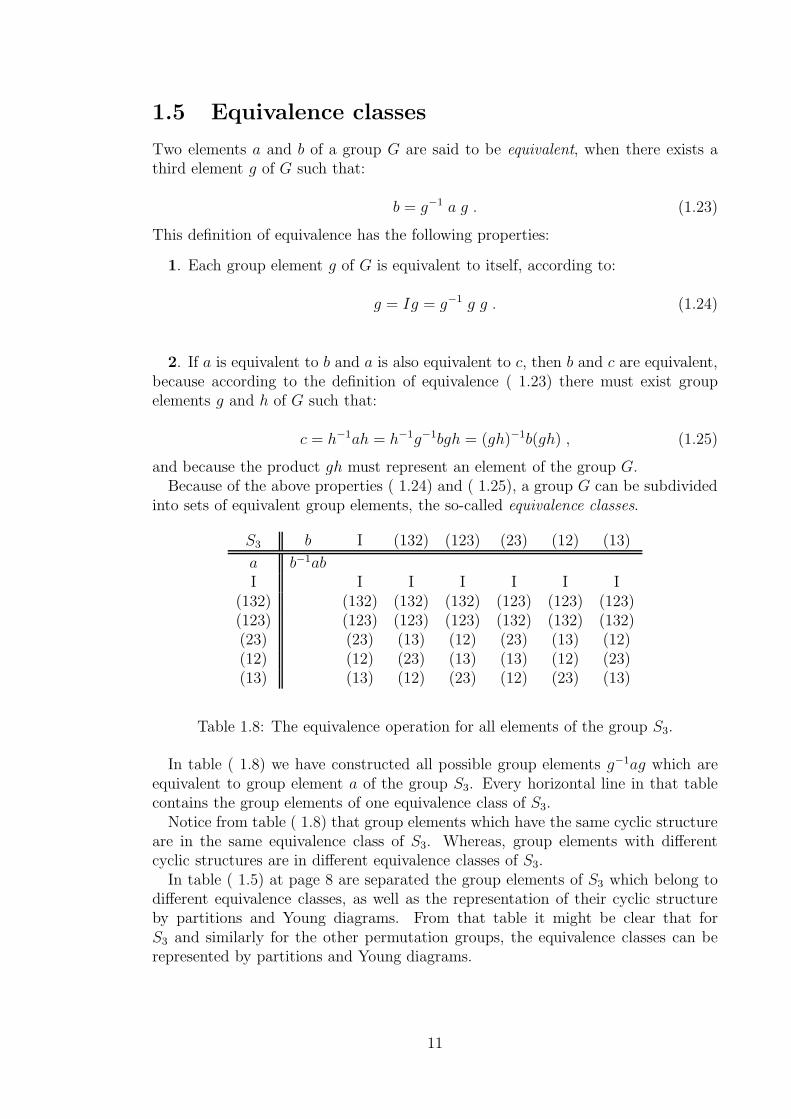
1.5 Equivalence classes
Two elements a and b of a group G are said to be equivalent, when there exists athird element g of G such that:
b = g−1 a g . (1.23)
This definition of equivalence has the following properties:
1. Each group element g of G is equivalent to itself, according to:
g = Ig = g−1 g g . (1.24)
2. If a is equivalent to b and a is also equivalent to c, then b and c are equivalent,because according to the definition of equivalence ( 1.23) there must exist groupelements g and h of G such that:
c = h−1ah = h−1g−1bgh = (gh)−1b(gh) , (1.25)
and because the product gh must represent an element of the group G.Because of the above properties ( 1.24) and ( 1.25), a group G can be subdivided
into sets of equivalent group elements, the so-called equivalence classes.
S3 b I (132) (123) (23) (12) (13)
a b−1abI I I I I I I
(132) (132) (132) (132) (123) (123) (123)(123) (123) (123) (123) (132) (132) (132)(23) (23) (13) (12) (23) (13) (12)(12) (12) (23) (13) (13) (12) (23)(13) (13) (12) (23) (12) (23) (13)
Table 1.8: The equivalence operation for all elements of the group S3.
In table ( 1.8) we have constructed all possible group elements g−1ag which areequivalent to group element a of the group S3. Every horizontal line in that tablecontains the group elements of one equivalence class of S3.Notice from table ( 1.8) that group elements which have the same cyclic structure
are in the same equivalence class of S3. Whereas, group elements with differentcyclic structures are in different equivalence classes of S3.In table ( 1.5) at page 8 are separated the group elements of S3 which belong to
different equivalence classes, as well as the representation of their cyclic structureby partitions and Young diagrams. From that table it might be clear that forS3 and similarly for the other permutation groups, the equivalence classes can berepresented by partitions and Young diagrams.
11

As an example of an other permutation group, we collect in table ( 1.9) theequivalence classes and their representations by partitions and Young diagrams ofthe group S4.
Equivalence class partition Young diagram
(1)(2)(3)(4) [1111]
(1)(2)(34) (1)(23)(4) (1)(24)(3)(12)(3)(4) (13)(2)(4) (14)(2)(3)
[211]
(12)(34) (13)(24) (14)(23) [22]
(1)(234) (1)(243) (123)(4) (132)(4)(124)(3) (142)(3) (134)(2) (143)(2)
[31]
(1234) (1243) (1324)(1342) (1423) (1432)
[4]
Table 1.9: The equivalence classes and their representation by partitions and Youngdiagrams of the permutation group S4.
12

Chapter 2
Representations of finite groups.
In this chapter we will discuss the definition and the properties of matrix represen-tations of finite groups.
2.1 What is a matrix representation of a group?
An n-dimensional matrix representation of a group element g of the group G, isgiven by a transformation D(g) of an n-dimensional (complex) vector space Vn intoitself, i.e.:
D(g) : Vn → Vn. (2.1)
The matrix for D(g) is known, once the transformation of the basis vectors ei(i = 1, · · · , n) of Vn is specified.
2.2 The word-representation D(w) of S3.
Instead of the ”three-letter” words introduced in section (1.1), we represent thosewords here by vectors of a three-dimensional vector space, i.e.:
ABC ⇒
ABC
= A
100
+B
010
+ C
001
. (2.2)
Moreover, the operations ( 1.12) are ”translated” into vector transformations. Forexample, the operation of (12) on a ”three-letter” word, given in ( 1.3), is heretranslated into the transformation:
D(w)((12))
ABC
=
BAC
. (2.3)
Then, assuming arbitrary (complex) values for A, B and C, the transformations
D(w)(g) can be represented by matrices. In the above example one finds:
13

D(w)((12)) =
0 1 01 0 00 0 1
. (2.4)
Similarly, one can represent the other operations of S3 by matrices D(w)(g). Intable ( 2.1) below, the result is summarized.
g D(w)(g) g D(w)(g) g D(w)(g)
I
1 0 00 1 00 0 1
(132)
0 1 00 0 11 0 0
(123)
0 0 11 0 00 1 0
(23)
1 0 00 0 10 1 0
(12)
0 1 01 0 00 0 1
(13)
0 0 10 1 01 0 0
Table 2.1: The word-representation D(w) of S3.
The structure of a matrix representation D of a group G reflects the structureof the group, i.e. the group product is preserved by the matrix representation.Consequently, we have for any two group elements a and b ofG the following propertyof their matrix representations D(a) and D(b):
D(a)D(b) = D(ab). (2.5)
For example, for D(w) of S3, using table ( 2.1) for the word-representation andmultiplication table ( 1.3) at page 5, we find for the group elements (12) and (23):
D(w)((12))D(w)((23)) =
0 1 01 0 00 0 1
1 0 00 0 10 1 0
=
0 0 11 0 00 1 0
= D(w)((123)) = D(w)((12)(23)). (2.6)
Notice from table ( 2.1) that all group elements of S3 are represented by a differentmatrix. A representation with that property is called a faithful representation.Notice also from table ( 2.1) that I is represented by the unit matrix. This is
always the case, for any representation.
14

2.3 The regular representation.
In the regular representation D(r) of a finite group G, the matrix which representsa group element g is defined in close analogy with the product operation of g onall elements of the group. The dimension of the vector space is in the case of theregular representation equal to the order p of the group G. The elements ei of theorthonormal basis e1, · · · , ep of the vector space are somehow related to the groupelements gi of G.
The operation of the matrix which represents the transformation D(r)(gk) on abasis vector ej is defined as follows:
D(r)(gk) ej =p∑
i = 1δ(gkgj, gi)ei, (2.7)
where the ”Kronecker delta function” is here defined by:
δ(gkgj, gi) =
1 if gkgj = gi
0 if gkgj 6= gi
.
Let us study the regular representation for the group S3. Its dimension is equalto the order of S3, i.e. equal to 6. So, each element g of S3 is represented by a 6× 6
matrix D(r)(g).
For the numbering of the group elements we take the one given in table ( 1.1) atpage 1.
As an explicit example, let us construct the matrix D(r)(g3 = (123)). From themultiplication table ( 1.2) at page 3 we have the following results:
g3g1 = g3 , g3g2 = g1 , g3g3 = g2 ,g3g4 = g5 , g3g5 = g6 , g3g6 = g4 .
Using these results and formula ( 2.7), we find for the orthonormal basis vectorsei of the six-dimensional vector space, the set of transformations:
D(r)(g3)e1 = e3
D(r)(g3)e2 = e1
D(r)(g3)e3 = e2
D(r)(g3)e4 = e5
D(r)(g3)e5 = e6
D(r)(g3)e6 = e4. (2.8)
Consequently, the matrix which belongs to this set of transformations, is givenby:
15

D(r)(g3) =
0 1 0 0 0 00 0 1 0 0 01 0 0 0 0 00 0 0 0 0 10 0 0 1 0 00 0 0 0 1 0
. (2.9)
The other matrices can be determined in a similar way. The resulting regular
representation D(r) of S3 is shown in table ( 2.2) below.
g D(r)(g) g D(r)(g)
I
1 0 0 0 0 00 1 0 0 0 00 0 1 0 0 00 0 0 1 0 00 0 0 0 1 00 0 0 0 0 1
(23)
0 0 0 1 0 00 0 0 0 1 00 0 0 0 0 11 0 0 0 0 00 1 0 0 0 00 0 1 0 0 0
(132)
0 0 1 0 0 01 0 0 0 0 00 1 0 0 0 00 0 0 0 1 00 0 0 0 0 10 0 0 1 0 0
(12)
0 0 0 0 1 00 0 0 0 0 10 0 0 1 0 00 0 1 0 0 01 0 0 0 0 00 1 0 0 0 0
(123)
0 1 0 0 0 00 0 1 0 0 01 0 0 0 0 00 0 0 0 0 10 0 0 1 0 00 0 0 0 1 0
(13)
0 0 0 0 0 10 0 0 1 0 00 0 0 0 1 00 1 0 0 0 00 0 1 0 0 01 0 0 0 0 0
Table 2.2: The regular representation D(r) of S3.
Notice from table ( 2.2) that, as in the previous case, each group element of S3
is represented by a different matrix. The regular representation is thus a faithfulrepresentation.From formula ( 2.7) one might deduce the following general equation for the matrix
elements of the regular representation of a group:
[
D(r)(gk)]
ij= δ(gkgj, gi). (2.10)
16

2.4 The symmetry group of the triangle.
In this section we study those transformations of the 2-dimensional plane into itself,which leave invariant the equilateral triangle shown in figure ( 2.1).
x
y
""""""""
""""""""
bbbbbbbb
bbbbbbbb
··
·
(a)
and x
y
TTTTT
TTTTT
-
6e2
e1·
·
·(
−1
0
)
(1/2
√3/2
)
(1/2
−√3/2
)
(b)
Figure 2.1: The equilateral triangle in the plane. The centre of the triangle (a) coin-cides with the origin of the coordinate system. In (b) are indicated the coordinatesof the corners of the triangle and the unit vectors in the plane.
A rotation, R, of 120 of the plane maps the triangle into itself, but maps theunit vectors e1 and e2 into e′1 and e′2 as is shown in figure ( 2.2).From the coordinates of the transformed unit vectors, one can deduce the matrix
for this rotation, which is given by:
R =
−1/2 −√3/2
√3/2 −1/2
. (2.11)
Twice this rotation (i.e. R2) also maps the triangle into itself. The matrix forthat operation is given by:
R2 =
−1/2√3/2
−√3/2 −1/2
. (2.12)
Three times (i.e. R3) leads to the identity operation, I.Reflection, P , around the x-axis also maps the triangle into itself. In that case
the unit vector e1 maps into e1 and e2 maps into −e2. So, the matrix for reflectionaround the x-axis is given by:
P =
1 0
0 −1
. (2.13)
17

x
y
""""""""
""""""""
bbbbbbbb
bbbbbbbb
··
·
(a)
and x
y
TT
TTT
TT
TTT
"""""
"""""
·
·
e′1
e′2
(b)
Figure 2.2: The effect of a rotation of 120 of the plane: In (a) the transformedtriangle is shown. In (b) are indicated the transformed unit vectors.
The other possible invariance operations for the triangle of figure ( 2.1) at page17 are given by:
PR =
−1/2 −√3/2
−√3/2 1/2
and PR2 =
−1/2√3/2
√3/2 1/2
. (2.14)
This way we obtain the six invariance operations for the triangle, i.e.:
I, R,R2, P, PR, PR2
. (2.15)
Now, let us indicate the corners of the triangle of figure ( 2.1) at page 17 by theletters A, B and C, as indicated in figure ( 2.3) below.
""""
bbbb
C
B
A
Figure 2.3: The position of the corners A, B and C of the triangle.
Then, the invariance operations ( 2.15) might be considered as rearrangements ofthe three letters A, B and C.
18

For example, with respect to the positions of the corners, the rotation R definedin formula ( 2.11) is represented by the rearrangement of the three letters A, B andC which is shown in figure ( 2.4).
""""
bbbb
C
B
A
-R
""""
bbbb
A
C
B
ABC BCA
Figure 2.4: The position of the corners A, B and C of the triangle after a rotationof 120.
We notice, that with respect to the order of the letters A, B and C, a rotation of120 has the same effect as the operation (132) of the permutation group S3 (compareformula 1.3). Consequently, one may view the matrix R of equation ( 2.11) as atwo-dimensional representation of the group element (132) of S3.
Similarly, one can compare the other group elements of S3 with the above trans-formations ( 2.15). The resulting two-dimensional representation D(2) of the per-mutation group S3 is shown in table ( 2.3) below.
g D(2)(g) g D(2)(g)
I
1 0
0 1
(23)
−1/2√3/2
√3/2 1/2
(132)
−1/2 −√3/2
√3/2 −1/2
(12)
1 0
0 −1
(123)
−1/2√3/2
−√3/2 −1/2
(13)
−1/2 −√3/2
−√3/2 1/2
Table 2.3: The two-dimensional representation D(2) of S3.
Notice that D(2) is a faithful representation of S3.
19

2.5 One-dimensional and trivial representations.
Every group G has an one-dimensional trivial representation D(1) for which eachgroup element g is represented by 1, i.e.:
D(1)(g)e1 = e1. (2.16)
This representation satisfies all requirements for a (one-dimensional) matrix rep-resentation.For example: if gigj = gk, then
D(1)(gi)D(1)(gj) = 1 · 1 = 1 = D(1)(gk) = D(1)(gigj),
in agreement with the requirement formulated in equation ( 2.5).For the permutation groups Sn exists yet another one-dimensional representation
D(1′), given by:
D(1′)(g) =
1 for even permutations−1 for odd permutations
. (2.17)
Other groups might have other (complex) one-dimensional representations. Forexample the subgroup A3 of even permutations of S3 can be represented by thefollowing complex numbers:
D(I) = 1 , D((132)) = e2πi/3 and D((123)) = e−2πi/3 , (2.18)
or also by the non-equivalent representation, given by:
D(I) = 1 , D((132)) = e−2πi/3 and D((123)) = e2πi/3 . (2.19)
20
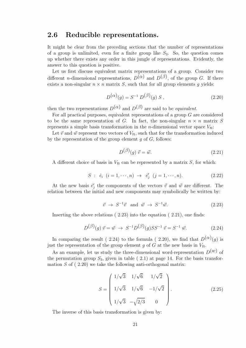
2.6 Reducible representations.
It might be clear from the preceding sections that the number of representationsof a group is unlimited, even for a finite group like S3. So, the question comesup whether there exists any order in this jungle of representations. Evidently, theanswer to this question is positive.
Let us first discuss equivalent matrix representations of a group. Consider two
different n-dimensional representations, D(α) and D(β), of the group G. If thereexists a non-singular n× n matrix S, such that for all group elements g yields:
D(α)(g) = S−1 D(β)(g) S , (2.20)
then the two representations D(α) and D(β) are said to be equivalent.
For all practical purposes, equivalent representations of a group G are consideredto be the same representation of G. In fact, the non-singular n × n matrix Srepresents a simple basis transformation in the n-dimensional vector space Vn:
Let ~v and ~w represent two vectors of Vn, such that for the transformation inducedby the representation of the group element g of G, follows:
D(β)(g) ~v = ~w. (2.21)
A different choice of basis in Vn can be represented by a matrix S, for which:
S : ei (i = 1, · · · , n) → e′j (j = 1, · · · , n). (2.22)
At the new basis e′j the components of the vectors ~v and ~w are different. Therelation between the initial and new components may symbolically be written by:
~v → S−1~v and ~w → S−1 ~w. (2.23)
Inserting the above relations ( 2.23) into the equation ( 2.21), one finds:
D(β)(g) ~v = ~w → S−1D(β)(g)SS−1 ~v = S−1 ~w. (2.24)
In comparing the result ( 2.24) to the formula ( 2.20), we find that D(α)(g) isjust the representation of the group element g of G at the new basis in Vn.
As an example, let us study the three-dimensional word-representation D(w) ofthe permutation group S3, given in table ( 2.1) at page 14. For the basis transfor-mation S of ( 2.20) we take the following anti-orthogonal matrix:
S =
1/√3 1/
√6 1/
√2
1/√3 1/
√6 −1/
√2
1/√3 −
√
2/3 0
. (2.25)
The inverse of this basis transformation is given by:
21

S−1 =
1/√3 1/
√3 1/
√3
1/√6 1/
√6 −
√
2/3
1/√2 −1/
√2 0
. (2.26)
For each group element g of S3 we determine the representation given by:
D(wS)(g) = S−1 D(w)(g) S , (2.27)
which is equivalent to the word-representation of S3. The result is collected in table( 2.4) below.
g S−1D(w)(g)S g S−1D(w)(g)S
I
1 0 0
0 1 0
0 0 1
(23)
1 0 0
0 −1/2√3/2
0√3/2 1/2
(132)
1 0 0
0 −1/2 −√3/2
0√3/2 −1/2
(12)
1 0 0
0 1 0
0 0 −1
(123)
1 0 0
0 −1/2√3/2
0 −√3/2 −1/2
(13)
1 0 0
0 −1/2 −√3/2
0 −√3/2 1/2
Table 2.4: The three-dimensional representation D(wS) = S−1D(w)S of S3.
From the table ( 2.4) for the three-dimensional representation which is equivalentto the word-representation of S3 shown in table ( 2.1) at page 14, we observe thefollowing:
1. For all group elements g of S3 their representation D(wS)(g) = S−1D(w)(g)Shas the form:
22

D(wS)(g) = S−1D(w)(g)S =
1 0 00 2× 20 matrix
. (2.28)
2. The 2 × 2 submatrices of the matrices D(wS)(g) = S−1D(w)(g)S shown intable ( 2.4) are equal to the two-dimensional representations D(2)(g) of the groupelements g of S3 as given in table ( 2.3) at page 19.
As a consequence of the above properties, the 3-dimensional word-representation
D(w) of S3 can be subdivided into two sub-representations of S3.In order to show this we take the following orthonormal basis for the three-
dimensional vector space V3 of the word representation:
a =
1/√3
1/√3
1/√3
, e1 =
1/√6
1/√6
−√
2/3
, e2 =
1/√2
−1/√2
0
. (2.29)
For this basis, using table ( 2.1) at page 14, we find for all group elements g ofS3, that:
D(w)(g) a = a = D(1)(g)a . (2.30)
Consequently, at the one-dimensional subspace of V3 which is spanned by the basisvector a, the word-representation is equal to the trivial representation ( 2.16).At the two-dimensional subspace spanned by the basis vectors e1 and e2 of ( 2.29),
one finds for vectors ~v defined by:
~v = v1e1 + v2e2 =
v1
v2
, (2.31)
that for all group elements g of S3 yields:
D(w)(g)~v = D(2)(g)
v1
v2
. (2.32)
For example:
D(w)((123))~v =
0 0 11 0 00 1 0
v1
1/√6
1/√6
−√
2/3
+ v2
1/√2
−1/√2
0
23

= v1
−√
2/3
1/√6
1/√6
+ v2
0
1/√2
−1/√2
= (−1
2v1 +
√3
2v2)e1 + (−
√3
2v1 −
1
2v2)e2
=
−1/2√3/2
−√3/2 −1/2
v1
v2
= D(2)((123))~v . (2.33)
For the other group elements g of S3 one may verify that D(w)(g) also satisfies( 2.32).
In general, an n-dimensional representation D(α) of the group G on a complexvector space Vn is said to be reducible if there exists a basis transformation S in Vnsuch that for all group elements g of G yields:
S−1D(α)(g)S =
D(a)(g) 0 0 · · · 0
0 D(b)(g) 0 · · · 0
......
......
0 0 0 · · · D(z)(g)
, (2.34)
where D(a), D(b), · · ·, D(z) are representations of dimension smaller than n, suchthat:
dim(a) + dim(b) + · · ·+ dim(z) = n. (2.35)
The vector space Vn can in that case be subdivided into smaller subspaces Vα(α=a, b, . . ., z) in each of which D(α)(g) is represented by a matrix which has adimension smaller than n, for all group elements g of G. If one selects a vector ~vαin one of the subspaces Vα, then the transformed vector ~vα, g = D(α)(g)~vα is alsoa vector of the same subspace Vα for any group element g of G.
24

2.7 Irreducible representations (Irreps).
An n-dimensional representation D(β) of a group G which cannot be reduced bythe procedure described in the previous section ( 2.6), is said to be irreducible.Irreducible representations or irreps are the building blocks of representations.
Other representations can be constructed out of irreps, following the procedureoutlined in the previous section and summarized in formula ( 2.34).The two-dimensional representation D(2) of S3 given in table ( 2.3) at page 19
is an example of an irreducible representation of the permutation group S3. Otherexamples of irreps of S3 are the trivial representation D(1) given in equation ( 2.16)and the one-dimensional representation D(1′) given in equation ( 2.17).The one-dimensional representations D(1) and the ones shown in equations ( 2.18)
and ( 2.19) are irreps of the group A3 defined in table ( 1.6) at page 9.If D is an irrep of the group G = g1, . . . , gp in the vector space V , then for any
arbitrary vector ~v in V the set of vectors ~v1 = D(g1)~v, . . . , ~vn = D(gn)~v may notform a subspace of V but must span the whole vector space V .
2.8 Unitary representations.
One may always restrict oneself to unitary representations, since according to thetheorem of Maschke:
Each representation is equivalent to an unitary representation. (2.36)
A representation D is an unitary representation of a group G when all groupelements g of G are represented by unitary matrices D(g). A matrix A is said to beunitary when its inverse equals its complex conjugated transposed, i.e.:
A†A = AA† = 1. (2.37)
Instead of proving the theorem of Maschke ( 2.36) we just construct an unitaryequivalent representation for an arbitrary representation D of a group G of order p.First recall the following properties of matrix multiplication:
(AB)† = B†A† and (AB)−1 = B−1A−1 . (2.38)
Next, let us study the matrix T , given by:
T =p∑
k = 1
D†(gk)D(gk) . (2.39)
One can easily verify, using ( 2.38), that this matrix is Hermitean, i.e.:
T † =p∑
k = 1
D†(gk)D(gk)† =
p∑
k = 1
D†(gk)D(gk) = T .
It moreover satisfies the following property (using once more 2.38):
25

D†(gi)TD(gi) =p∑
k = 1
D†(gi)D†(gk)D(gk)D(gi) =
p∑
k = 1
D†(gkgi)D(gkgi)
=p∑
j = 1D†(gj)D(gj) = T , (2.40)
where we also used the fact that in multiplying one particular group element gi withall group elements gk (k = 1, . . . p), one obtains all group elements gj only once.Next, we define a basis transformation S such that:
1. S† = S, and 2. S2 = T−1.
S represents a transformation from a basis orthonormal with respect to the scalarproduct given by:
( ~x , ~y ) =
p
Σj = 1
⟨
D(gj)~x ||D(gj)~y⟩
,
to a basis orthonormal with respect to the scalar product given by:
〈~x || ~y〉 .
With the definition of S the property ( 2.40) can be rewritten by:
D†(gi)S−2D(gi) = S−2 .
Multiplying this line from the right by D−1(gi)S and from the left by S, one obtains:
SD†(gi)S−1 = S−1D−1(gi)S ,
which, using the fact that S is Hermitean and using ( 2.38), finally gives:
(S−1D(gi)S)† = (S−1D(gi)S)
−1 .
Leading to the conclusion that the matrix representation S−1DS, equivalent to D,is unitary.As a consequence of ( 2.36) and because of the fact that equivalent representations
are considered the ”same” representations as discussed in section ( 2.6), we may inthe following restrict ourselves to unitary representations of groups.
One can easily verify that D(1), D(1′), D(2), D(w), D(wS) and D(r) are unitaryrepresentations of S3.
26

Chapter 3
The standard irreps of Sn.
In this chapter we will discuss the standard construction of irreps for the symmetricgroups Sn.
3.1 Standard Young tableaux and their associ-
ated Yamanouchi symbols.
A Young tableau is a Young diagram (see section ( 1.3) at page 8 for the definitionof a Young diagram), of n boxes filled with n numbers in some well specified way.A standard Young tableau is a Young diagram of n boxes which contains the
numbers 1 to n in such a way that the numbers in each row increase from the leftto the right, and in each column increase from the top to the bottom.For S3, using the result of table ( 1.5) at page 8, one finds four different possible
standard Young tableaux, i.e.:
321
, 1 2 3 , 13
2and
123 .
(3.1)
Notice that one Young diagram in general allows for several different standard Youngtableaux.Each standard tableau can be denoted in a compact and simple way by a Ya-
manouchi symbol, M = M1,M2, · · · ,Mn. This is a row of n numbers Mi (i =1, · · · , n), where Mi is the number of the row in the standard Young tableau, count-ing from above, in which the number i appears. Below we show the Yamanouchisymbols corresponding to the standard Young tableaux for S3 given in ( 3.1):
321
1 in the 1st row
2 in the 2nd row
3 in the 3rd row
M = 123 ,
1 2 3
1 in the 1st row
2 in the 1st row
3 in the 1st row
M = 111 ,
27

13
2
1 in the 1st row
2 in the 1st row
3 in the 2nd row
M = 112 , and
12
3
1 in the 1st row
2 in the 2nd row
3 in the 1st row
M = 121 . (3.2)
There exists moreover a certain order in the Yamanouchi symbols for the sameYoung diagram: First one orders these symbols with respect to increasing values ofM1, then with respect to increasing values of M2, etc.Let us, as an example, order the Yamanouchi symbols for the standard Young
tableaux of the partition [µ] = [32] of the permutation group S5. The possibleYamanouchi symbols, properly ordered, are given by:
11122 , 11212 , 11221 , 12112 and 12121 .
3.2 Hooklength, hookproduct and axial distance.
Other quantities related to Young diagrams, are the hooklength of a box, thehookproduct and the axial distance between boxes.As the hook of a certain box j in a Young diagram, one defines a set of boxes
given by the following receipt:
1. The box j itself.2. All boxes to the right of j in the same row.3. All boxes below j in the same column.
(3.3)
As an example, we show below the hook of the first box in the second row of theYoung diagram belonging to the partition [433] of S10:
⋆⋆ ⋆ ⋆
As the hooklength of a certain box j in a Young diagram, one defines the numberof boxes in the hook of box j. In the above example one has a hooklength of 4.The hooktableau of a Young diagram is obtained by placing in each box of the
diagram, the hooklength of this box. For example, the hooktableau of the abovediagram [433] of S10, is given by:
3 2 14 3 26 5 4 1
The hookproduct h[µ] of the Young diagram belonging to the partition [µ], is theproduct of all numbers in its hooktableau. In the above example, [µ] = [433] of S10,one finds h[433] = 17280.
28

For the group S3, one has the following hooktableaux:
123
, 3 2 1 and31
1 .
(3.4)
The related hookproducts are h[111] = h[3] = 6 and h[21] = 3.
The axial distance ρ(M ; x, y) between two boxes x and y of a standard Youngtableau M (M represents the Yamanouchi symbol of the tableau), is the number ofsteps (horizontal and/or vertical) to get from x to y, where steps contribute:
+1 when going down or to the left,−1 when going up or to the right.
(3.5)
Notice that the axial distance does not depend on the path. Below we show as anexample the axial distances for the Young tableaux which belong to the partition[µ] = [21] of the permutation group S3.
13
2M = 112
ρ(112; 1, 2) = −ρ(112; 2, 1) = −1ρ(112; 1, 3) = −ρ(112; 3, 1) = +1ρ(112; 2, 3) = −ρ(112; 3, 2) = +2
12
3M = 121
ρ(121; 1, 2) = −ρ(121; 2, 1) = +1ρ(121; 1, 3) = −ρ(121; 3, 1) = −1ρ(121; 2, 3) = −ρ(121; 3, 2) = −2
(3.6)
3.3 The dimension of irreps for Sn.
In one of the following chapters we will see that the number of inequivalent irre-ducible representations for any finite group is equal to the number of equivalenceclasses of the group. Since, moreover, the different equivalence classes of Sn canbe represented by Young diagrams, it will not be surprising that also the differentirreps of Sn can be represented by Young diagrams. The dimension f [µ] of an irrepof Sn corresponding to a Young diagram [µ] (where [µ] represents the correspondingpartition of n) can be found from:
f [µ] = number of possible standard Young tableaux, (3.7)
or alternatively, from:
f [µ] =n!
h[µ], (3.8)
where h[µ] represents the hookproduct of the Young diagram [µ].
For S3, using formula ( 3.7) in order to count the various possible standard Youngtableaux of a partition (see ( 3.1)), or alternatively, using ( 3.8) for the hookproductsof the different Young diagrams of S3 (see ( 3.4)), one finds:
29

f [111] = 1, or alternatively f [111] =3!
6= 1,
f [3] = 1, or alternatively f [3] =3!
6= 1, and
f [21] = 2, or alternatively f [21] =3!
3= 2. (3.9)
3.4 Young’s orthogonal form for the irreps of Sn.
In section ( 1.2) we have seen at page 6 that the permutation group Sn can begenerated by the group elements (12) and (12 · · ·n) (see formula 1.17), or, alterna-tively, by the transpositions (12), (23), . . ., (n−1, n). Consequently, it is more thansufficient to determine the matrix representations for the transpositions (12), (23),. . ., (n − 1, n) of Sn. The matrix representation of the other elements of Sn canthen be obtained by (repeated) multiplication.As standard form we will use Young’s orthogonal form. These matrices are real
and unitary and therefore orthogonal.
The irrep [µ] of Sn is defined in an f [µ]-dimensional vector space V [µ]. In this
space we choose an orthonormal basis e[µ]i (i = 1, · · · , f [µ]), with:
(
e[µ]i , e
[µ]j
)
= δij for (i, j = 1, · · · , f [µ]). (3.10)
To the index i of the basisvector e[µ]i we relate the Yamanouchi symbol M in the
order which has been discussed in section ( 3.1) at page 27. So, alternatively wemay write:
e[µ]i = e
[µ]M , (3.11)
whereM corresponds to the i-th Yamanouchi symbol which belongs to the partition[µ].For example, for the two-dimensional representation [21] of S3, we have as a basis:
e[21]1 = e
[21]112 and e
[21]2 = e
[21]121 . (3.12)
In terms of the basis vectors e[µ]M one obtains the Young’s standard form for
the matrix representation D[µ]((k, k + 1)) of the transposition (k, k + 1) of thepermutation group Sn by the following transformation rule:
D[µ]((k, k + 1)) e[µ]M1 · · ·Mn = (ρ(M1 · · ·Mn; k + 1, k))−1 e
[µ]M1 · · ·Mn+
+√
1− (ρ(M1 · · ·Mn; k + 1, k))−2 e[µ]M1 · · ·Mk + 1Mk · · ·Mn
,
(3.13)
30

where ρ(M ; k + 1, k) represents the axial distance between box k + 1 and k in thestandard Young diagram corresponding to the Yamanouchi symbolM =M1 · · ·Mn.
3.5 The standard irreps of S3.
For the two-dimensional representation [21] of S3, one finds, using relation ( 3.13),the following:
D[21]((12))e[21]112 = e
[21]112 , and D[21]((12))e
[21]121 = −e[21]121 . (3.14)
So, when we represent the basis vector e[21]112 by the column vector
(
10
)
and the
basis vector e[21]121 by the column vector
(
01
)
, then the corresponding matrix is given
by:
D[21]((12)) =
(
1 00 −1
)
. (3.15)
For the transposition (23) one finds:
D[21]((23))e[21]112 = −1
2e[21]112 +
√3
2e[21]121 , and D[21]((23))e
[21]121 =
1
2e[21]121 +
√3
2e[21]112 . (3.16)
Consequently, the corresponding matrix is given by:
D[21]((23)) =
(
−1/2√3/2√
3/2 1/2
)
. (3.17)
These results might be compared to the matrix representation for the invariancegroup of the triangle given in table ( 2.3) at page 19.As far as the one-dimensional representations are concerned, one finds:
D[111]((12))e[111]123 = −e[111]123 , and D[111]((23))e
[111]123 = −e[111]123 . (3.18)
Consequently, [111] corresponds to the irrep D(1′), discussed in formula ( 2.17).Also:
D[3]((12))e[3]111 = e
[3]111, and D[3]((23))e
[3]111 = e
[3]111. (3.19)
So, [3] corresponds to the trivial irrep D(1) (see equation 2.16).
3.6 The standard irreps of S4.
For the symmetric group S4 we have five different partitions, i.e. [1111], [211], [22],[31] and [4] (see the table of equivalence classes of S4, table ( 1.9) at page 12), andconsequently five inequivalent irreducible representations. Let us first collect thenecessary ingredients for the construction of those irreps, i.e. the resulting Youngtableaux, Yamanouchi symbols and relevant axial distances, in the table below.
31

partition Young tableaux Yamanouchi symbols axial distances
[1111]1234
1234ρ(1234; 2, 1) = −1ρ(1234; 3, 2) = −1ρ(1234; 4, 3) = −1
[211]1 234
1123ρ(1123; 2, 1) = +1ρ(1123; 3, 2) = −2ρ(1123; 4, 3) = −1
1 324
1213ρ(1213; 2, 1) = −1ρ(1213; 3, 2) = +2ρ(1213; 4, 3) = −3
1 423
1231ρ(1231; 2, 1) = −1ρ(1231; 3, 2) = −1ρ(1231; 4, 3) = +3
[22] 1 23 4
1122ρ(1122; 2, 1) = +1ρ(1122; 3, 2) = −2ρ(1122; 4, 3) = +1
1 32 4
1212ρ(1212; 2, 1) = −1ρ(1212; 3, 2) = +2ρ(1212; 4, 3) = −1
[31] 1 2 34
1112ρ(1112; 2, 1) = +1ρ(1112; 3, 2) = +1ρ(1112; 4, 3) = −3
1 2 43
1121ρ(1121; 2, 1) = +1ρ(1121; 3, 2) = −2ρ(1121; 4, 3) = +3
1 3 42
1211ρ(1211; 2, 1) = −1ρ(1211; 3, 2) = +2ρ(1211; 4, 3) = +1
[4] 1 2 3 4 1111ρ(1111; 2, 1) = +1ρ(1111; 3, 2) = +1ρ(1111; 4, 3) = +1
Table 3.1: The Young tableaux, Yamanouchi symbols and axial distances for thevarious irreps of S4.
32

Using the results of table ( 3.1) and formula ( 3.13) one obtains the matrices whichare collected in table ( 3.2) below, for the three generator transpositions of S4.
irrep [1111] [211] [22] [31] [4]
basis e[1111]1234 e
[211]1123 =
100
e
[22]1122 =
(
10
)
e[31]1112 =
100
e
[4]1111
e[211]1213 =
010
e
[22]1212 =
(
01
)
e[31]1121 =
010
e[211]1231 =
001
e
[31]1211 =
001
D((12)) -1
1 0 00 −1 00 0 −1
(
1 00 −1
)
1 0 00 1 00 0 −1
+1
D((23)) -1
−12
√32
0√32
12
0
0 0 −1
−1
2
√32√
32
12
1 0 0
0 −12
√32
0√32
12
+1
D((34)) -1
−1 0 0
0 −13
√83
0√83
13
(
1 00 −1
)
−13
√83
0√83
13
0
0 0 1
+1
Table 3.2: Young’s orthogonal form for the irreps of the symmetric group S4 for thethree generator transpositions (12), (23) and (34).
For later use we will also determine the matrices for a representant of each ofthe equivalence classes of S4 which are shown in table ( 1.9) at page 12. The onlymember of [1111] is the identity operator I, which is always represented by the unitmatrix. For the equivalence class [211] one might select the transposition (12) asa representant. Its matrix representations for the five standard irreps are alreadyshown in table ( 3.2). As a representant of the equivalence class [22] we select theoperation (12)(34). Its matrix representations for the various standard irreps canbe determined, using the property formulated in equation ( 2.5) for representations,
33

i.e. D((12)(34)) = D((12))D((34)). The resulting matrices are collected in table( 3.3). For [31] we select the operation (123) = (12)(23) as a representant. Itsmatrix representations follow from D((123)) = D((12))D((23)) using the results oftable ( 3.2). Finally, for the equivalence class [4] we select the operation (1234) =(12)(23)(34). The resulting matrices are collected in table ( 3.3) below.
irrep D((12)(34)) D((123)) D((1234))
[1111] +1 +1 −1
[211]
−1 0 0
0 13
−√83
0 −√83
−13
−12
√32
0
−√32
−12
0
0 0 1
12
−√36
√63√
32
16
−√23
0√83
13
[22]
(
1 00 1
)
−1
2
√32
−√32
−12
−1
2−
√32
−√32
12
[31]
−13
√83
0√83
13
0
0 0 −1
1 0 0
0 −12
√32
0 −√32
−12
−13
√83
0
−√23
−16
√32
−√63
−√36
−12
[4] +1 +1 +1
Table 3.3: Young’s orthogonal form for the irreps of the symmetric group S4 forrepresentants of the three equivalence classes [22], [31] and [4].
34
Chapter 4
The classification of irreps.
In this chapter we discuss some properties of irreducible representations and studythe resulting classification of irreps for finite groups.
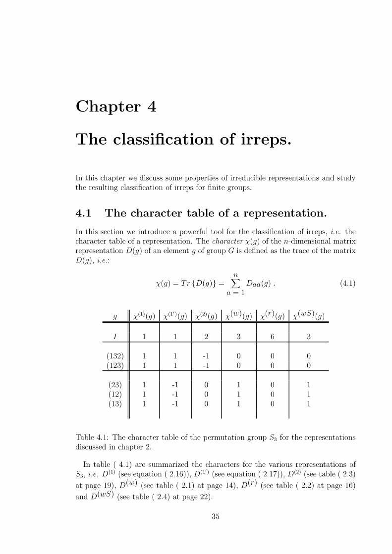
4.1 The character table of a representation.
In this section we introduce a powerful tool for the classification of irreps, i.e. thecharacter table of a representation. The character χ(g) of the n-dimensional matrixrepresentation D(g) of an element g of group G is defined as the trace of the matrixD(g), i.e.:
χ(g) = Tr D(g) =n∑
a = 1Daa(g) . (4.1)
g χ(1)(g) χ(1′)(g) χ(2)(g) χ(w)(g) χ(r)(g) χ(wS)(g)
I 1 1 2 3 6 3
(132) 1 1 -1 0 0 0(123) 1 1 -1 0 0 0
(23) 1 -1 0 1 0 1(12) 1 -1 0 1 0 1(13) 1 -1 0 1 0 1
Table 4.1: The character table of the permutation group S3 for the representationsdiscussed in chapter 2.
In table ( 4.1) are summarized the characters for the various representations ofS3, i.e. D
(1) (see equation ( 2.16)), D(1′) (see equation ( 2.17)), D(2) (see table ( 2.3)
at page 19), D(w) (see table ( 2.1) at page 14), D(r) (see table ( 2.2) at page 16)
and D(wS) (see table ( 2.4) at page 22).
35

In the following we will frequently use a property of the trace of a matrix, relatedto the trace of the product AB of two n× n matrices A and B, i.e.:
Tr AB =n∑
i = 1[AB]ii =
n∑
i = 1
n∑
j = 1AijBji
=n∑
j = 1
n∑
i = 1BjiAij =
n∑
j = 1[BA]jj = Tr BA . (4.2)
Several properties of characters may be noticed from the character table ( 4.1) atpage 35 of the permutation group S3.
1. The characters of the word-representation D(w) and its equivalent represen-
tation D(wS) are identical.This is not surprising, since for any two equivalent matrix representations D(β)
and D(α) = S−1D(β)S (see equation ( 2.20) for the definition of equivalent matrixrepresentations), one has for each group element g of the group G, using the property( 4.2) for the trace of a matrix, the identity:
χ(β)(g) = Tr
D(β)(g)
= Tr
S−1D(α)(g)S
= Tr
D(α)(g)
= χ(α)(g) .
(4.3)Consequently, any two equivalent representations have the same character table.
2. The character χ(I) of the identity operation I, indicates the dimension of therepresentation.In the following we will indicate the dimension n of an n-dimensional representa-
tion D(α) of the group G, by the symbol f(α) = n. From the character table ( 4.1)at page 35 for S3 we observe:
f(α) = χ(α)(I) . (4.4)
3. Group elements which belong to the same equivalence class (see section ( 1.5)for the definition of equivalence classes), have the same characters.This can easily be shown to be a general property of characters: Using formula
( 1.23) for the definition of two equivalent group elements a and b = g−1ag, equation( 2.5) for the representation of the product D(a)D(b) = D(ab) of group elementsand property ( 4.2) of the trace of a matrix, one finds:
χ(b) = Tr D(b) = Tr
D(g−1ag)
= Tr
D(g−1)D(a)D(g)
= Tr
D(a)D(g)D(g−1)
= Tr D(a)D(I) = Tr D(a)
= χ(a) . (4.5)
36

As a consequence, characters are functions of equivalence classes.
Given this property of representations, it is sufficient to know the character of onerepresentant for each equivalence class of a group, in order to determine the charactertable of a group. Using the tables ( 3.2) and ( 3.3) we determine the character tableof S4, which is shown below. The number of elements for each equivalence class canbe found in table ( 1.9) at page 12.
irrepsequivalence number of
classes elements [1111] [211] [22] [31] [4]χ χ χ χ χ
[1111] 1 +1 +3 +2 +3 +1[211] 6 −1 −1 0 +1 +1[22] 3 +1 −1 +2 −1 +1[31] 8 +1 0 −1 0 +1[4] 6 −1 +1 0 −1 +1
Table 4.2: The character table of the symmetry group S4 for the standard irreduciblerepresentations discussed in the previous chapter.
4. The characters of the word-representation D(w) are the sums of the charactersof the trivial representation D(1) and the two-dimensional representation D(2), i.e.for each group element g of S3 we find:
χ(w)(g) = χ(1)(g) + χ(2)(g) . (4.6)
The reason for the above property is, that the word-representation D(w) can bereduced to the direct sum of the trivial representation D(1) and the two-dimensionalrepresentation D(2) (see table ( 2.4) at page 22). So, the traces of the matrices
D(w)(g) are the sums of the traces of the sub-matrices D(1)(g) and D(2)(g).
The property ( 4.6) can be used to discover how a representation can be reduced.
For example, one might observe that for the regular representation D(r) one has foreach group element g of S3, the following:
χ(r)(g) = χ(1)(g) + χ(1′)(g) + 2× χ(2)(g) . (4.7)
This suggests that the 6× 6 regular representation can be reduced into one timethe trivial representation [3], one time the representation [111] and two times thetwo-dimensional representation [21], and that there exists a basis transformation Sin the six-dimensional vector space V6 defined in section ( 2.3), such that for eachgroup element g of S3 yields:
37

S−1D(r)(g)S =
D(1)(g) 0
0 D(1′)(g)
0 0
0 0
0 0
0 0
0 0
0 0D(2)(g)
0 0
0 0
0 0
0 0
0 0
0 0D(2)(g)
. (4.8)
Indeed, such matrix S can be found for the regular representation of S3, whichshows that the regular representation is reducible.For the 24×24 regular representation of S4, using table ( 4.2), one finds similarly:
χ(r)(g) = χ[1111](g) + 3χ[211](g) + 2χ[22](g) + 3χ[31](g) + χ[4](g) , (4.9)
where we also used the fact that the characters of the regular representation for anygroup vanish for all group elements except for the character of the identity operator.One might observe from the expressions ( 4.7) and ( 4.9) that each representation
appears as many times in the sum as the size of its dimension. This is generallytrue for the regular representation of any group, i.e.:
χ(r)(g) =∑
all irrepsf(irrep)χ(irrep)(g) .
For the identity operator I of a group of order p this has the following interestingconsequence:
p = χ(r)(I) =∑
all irreps
f(irrep)χ(irrep)(I) =∑
all irreps
f(irrep)2 . (4.10)
For example, the permutation group S3 has 6 elements. Its irreps are D(1) (seeequation ( 2.16)), D(1′) (see equation ( 2.17)) and D(2) (see table ( 2.3) at page 19),with respective dimensions 1, 1 and 2. So, we find for those irreps:
12 + 12 + 22 = 6,
which, using the above completeness relation ( 4.10), proofs that S3 has no moreinequivalent irreps.
4.2 The first lemma of Schur.
When, for an irrep D of a group G = g1, . . . , gp in a vector space V , a matrix Acommutes with D(g) (i.e. AD(g) = D(g)A) for all elements g of G, then the matrixA must be proportional to the unit matrix, i.e.:
38

A = λ1 for a complex (or real) constant λ. (4.11)
This is Schur’s first lemma.As an example, let us study the 2× 2 irrep D[21] of S3 (see section ( 3.5) at page
31). We define the matrix A by:
A =
a11 a12
a21 a22
.
First, we determine the matrix products AD[21]((12)) and D[21]((12))A, to find thefollowing result:
AD[21]((12)) =
a11 −a12
a21 −a22
and D[21]((12))A =
a11 a12
−a21 −a22
.
Those two matrices are equal under the condition that a12 = a21 = 0. So, we areleft with the matrix:
A =
a11 0
0 a22
.
Next, we determine the matrix products AD[21]((23)) and D[21]((23))A, to obtain:
AD[21]((23)) =
−a112a11
√3
2
a22√3
2a222
and D[21]((23))A =
−a112a22
√3
2
a11√3
2a222
.
Those two matrices are equal under the condition that a11 = a22. So, we finally endup with the matrix:
A = a111
in agreement with the above lemma of Schur.
The condition that the representation is irreducible can be shown to be a necessarycondition by means of the following example: Let us consider the reducible wordrepresentation of S3. From the matrices shown in table ( 2.1) at page 14 it is easyto understand that the matrix A given by:
A =
a a aa a aa a a
commutes with all six matrices but is not proportional to the unit matrix.
39

Proof of Schur’s first lemma:
Let ~r be an eigenvector in V of A with eigenvalue λ. Since D is an irrep of G, theset of vectors ~r1 = D(g1)~r, . . . , ~rp = D(gp)~r must span the whole vector spaceV , which means that each vector of V can be written as a linear combination ofthe vectors ~r1, . . ., ~rp. But, using the condition that A commutes with D(g) for allelements g of G, one has also the relation:
A~ra = AD(ga)~r = D(ga)A~r = D(ga)λ~r = λ~ra , (a = 1, . . . , p) .
Consequently, all vectors in V are eigenvectors of A with the same eigenvalue λ,which leads automatically to the conclusion ( 4.11).
4.3 The second lemma of Schur.
Let D(1) represent an n1 × n1 irrep of a group G = g1, . . . , gp in a n1-dimensionalvector space V1 and D(2) an n2 × n2 irrep of G in a n2-dimensional vector space V2.Let moreover A represent an n2 × n1 matrix describing transformations from V1 onto V2. When for all group elements g of G yields AD(1)(g) = D(2)(g)A, then:
either A = 0
or n1 = n2 and det(A) 6= 0 .(4.12)
In the second case are moreover D(1) and D(2) equivalent.
For an example let us study the irreps D[211] and D[22] of the symmetric group S4
(see table ( 3.2) at page 33) and the matrix A given by:
A =
a11 a12a21 a22a31 a32
.
First, we determine the matrix products D[211]((12))A and AD[22]((12)), to find thefollowing result:
D[211]((12))A =
a11 a12
−a21 −a22
−a31 −a32
and AD[22]((12)) =
a11 −a12
a21 −a22
a31 −a32
.
Those two matrices are equal under the condition that a12 = a21 = a31 = 0. So, weare left with the matrix:
A =
a11 00 a220 a32
.
Next, we determine the matrix products D[211]((23))A and AD[22]((23), to obtain:
40

D[211]((23))A =
−a112a22
√3
2
a11√3
2a222
0 −a32
and AD[22]((23)) =
−a112a11
√3
2
a22√3
2a222
a32√3
2a322
.
Those two matrices are equal under the conditions that a11 = a22 and a32 = 0. So,we are left with the matrix:
A =
a11 00 a110 0
.
Finally, we determine the matrix products D[211]((34))A and AD[22]((34), to get:
D[211]((34))A =
−a11 0
0 −a113
0 0
and AD[22]((34)) =
a11 0
0 −a11
0 0
.
Those two matrices are equal when a11 = 0. So, we end up A = 0 in accordancewith the second lemma of Schur.
Proof of Schur’s second lemma.
We consider separately the two cases n1 ≤ n2 and n1 > n2:
(i) n1 ≤ n2
For ~r an arbitrary vector in the vector space V1, A~r is a vector in V2. The subspaceVA of V2 spanned by all vectors A~r for all possible vectors in V1, has a dimensionnA which is smaller or equal to n1, i.e.:
nA ≤ n1 ≤ n2 .
Let us choose one vector ~v = A~r (for ~r in V1) out of the subspace VA of V2. Thetransformed vector ~va under the transformation D(2)(ga) satisfies:
~va = D(2)(ga)~v = D(2)(ga)A~r = AD(1)(ga)~r = A~ra ,
where ~ra is a vector of V1. Consequently, the vector ~va must be a vector of VA.So, the set of vectors ~v1 = D(2)(g1)~v, . . . , ~vp = D(2)(gp)~v spans the vector
subspace VA of V2. However, since D(2) is an irrep, we must have VA = V2, unlessA = 0. Consequently, we find:
nA = n1 = n2 or A = 0 .
41

In the case that n1 = n2 we may consider V1 = V2 for all practical purposes. Whenmoreover, A 6= 0, the matrix A has an inverse, because then VA = V2 = V1, whichgives D(1)(g) = A−1D(2)(g)A for all group elements g of G and so D(1) and D(2) areequivalent.
(ii) n1 > n2
In that case there must exist vectors ~r in V1 which are mapped on to zero in V2by A, i.e. A~r = 0. The subspace V ′
A of vectors ~r in V1 which are mapped on to zeroin V2 has a dimension n′
A smaller than or equal to n1. Now, if ~r belongs to V′A, then
~ra = D(1)(ga)~r also belongs to V ′A, according to:
A~ra = AD(1)(ga)~r = D(2)(ga)A~r = 0 .
This contradicts the irreducibility of D(1), unless n′A = n1, in which case A = 0.
4.4 The orthogonality theorem.
Let D(i) represent an ni×ni irrep of a group G = g1, . . . , gp of order p, and D(j)
an nj × nj irrep of G. Let moreover D(i) either not be equivalent to D(j) or be
equal to D(j). Then:
∑
all g
[
D(i)(g)]∗ab
[
D(j)(g)]
cd=
p
niδijδacδbd (4.13)
Proof
Let X be a nj × ni matrix, then we define the matrix A as follows:
A =p∑
k = 1D(j)(gk)XD
(i)(g−1
k ) . (4.14)
This matrix has the property D(j)(ga)A = AD(i)(ga) as can easily be verified, usingthe relation ( 2.5) and the fact that D(g−1)D(g) = D(I) = 1. Consequently,
according to the second lemma of Schur ( 4.12) either A = 0 or D(i) and D(j) areequivalent. Remember that in case the two irreps are equivalent we assume thatthey are equal. When the two irreps are equal one has that according to the firstlemma of Schur ( 4.11) A = λ1. One might combine the two possibilities for A into:
A = λδij1 =
0 for D(i) 6= D(j)
λ1 for D(i) = D(j)(4.15)
The value of λ depends on the choice of the matrix X . Let us select matrices Xwhich have zero matrix elements all but one. The nonzero matrix element equals1 and is located at the intersection of the d-th row and the b-th column. For suchmatrices X one finds, using ( 4.14) and ( 4.15):
42

λδijδca = [A]ca
=p∑
k = 1
nj∑
α = 1
ni∑
β = 1
[D(j)(gk)]cαXαβ [D(i)(g−1
k )]βa
=p∑
k = 1
nj∑
α = 1
ni∑
β = 1
[D(j)(gk)]cαδαdδbβ [D(i)(g−1
k )]βa
=p∑
k = 1
[D(j)(gk)]cd[D(i)(g−1
k )]ba (4.16)
The value of λ is only relevant when i = j and a = c. In that case we take the sumover both sides of ( 4.16) in a, leading to:
λni =ni∑
a = 1λδiiδaa
=ni∑
a = 1
p∑
k = 1
[D(i)(gk)]ad[D(i)(g−1
k )]ba
=p∑
k = 1[D(i)(I)]bd
= pδbd
Inserting this result for λ in ( 4.16) and using the fact that for a unitary represen-tation D(g−1) = D−1(g) = D†(g), one obtains the relation ( 4.13).
4.5 The orthogonality of characters for irreps.
Let us define for the representation D(α) of a group G of order p and with elements
g1, · · · , gp, the following (complex) column vector ~χ (α) of length p:
~χ (α) =
χ(α)(g1)...
χ(α)(gp)
. (4.17)
In the following we will refer to such vectors as the character of the representation
D(α) of G.
We define moreover, the (complex) innerproduct of characters by:
43

(
~χ (α) , ~χ (β))
=p∑
i = 1
~χ (α)(gi)∗
~χ (β)(gi) . (4.18)
Let us concentrate on the characters of the irreps D(1), D(1′) and D(2) of S3 (seetable ( 4.1) at page 35, given by the three following six-component vectors:
~χ (1) =
111111
, ~χ (1′) =
111
−1−1−1
and ~χ (2) =
2−1−1000
. (4.19)
First, we notice for those three characters, using the definition ( 4.18) of theinnerproduct for characters, the property:
(
~χ (1) , ~χ (1))
=(
~χ (1′) , ~χ (1′))
=(
~χ (2) , ~χ (2))
= 6 ,
which result is equal to the order of the permutation group S3. Furthermore, wenotice that:
(
~χ (1) , ~χ (1′))
=(
~χ (1′) , ~χ (2))
=(
~χ (2) , ~χ (1))
= 0 .
Or, more compact, one might formulate the above properties for S3 as follows:
(
~χ (α) , ~χ (β))
= 6δαβ for α, β = 1, 1′ and 2. (4.20)
Consequently, the six-component vectors ( 4.19) form an orthogonal basis for athree-dimensional sub-space of all possible vectors in six dimensions.This can be shown to be true for any finite group. Using the property formulated
in equation ( 4.13), we obtain for two non-equivalent irreps (α) of dimension f(α)and (β) of dimension f(β) of a group G of order p , the following:
(
~χ (α) , ~χ (β))
=∑
g ∈ G
χ(α)(g)∗
χ(β)(g)
=∑
g ∈ GTr
D(α)(g)∗
Tr
D(β)(g)
=∑
g ∈ G
f(α)∑
a = 1
D(α)aa (g)
∗ f(β)∑
b = 1D(β)bb (g)
=
f(α)∑
a = 1
f(β)∑
b = 1
∑
g ∈ G
D(α)aa (g)
∗D(β)bb (g)
=
f(α)∑
a = 1
f(β)∑
b = 1
p
f(α)δαβ δab δab = pδαβ . (4.21)
44

Consequently, the characters for different (non-equivalent) irreps of a finite groupare orthogonal.
Next, we remember that the characters for group elements which belong to thesame equivalence class of S3, are equal (see formula ( 4.5)). So, all possible charactersof different representations (α) of S3 have the following form:
~χ (α) =
abbccc
,
where a = f(α) represents the dimension of the representation (α) of S3, where brepresents the trace of the matrix representation for either of the two equivalentsymmetric permutations of S3 and where c represents the trace of any of the threeequivalent antisymmetric permutations of S3.
However, such six-component vectors can be decomposed as linear combinationsof the three basis vectors ( 4.19), according to:
~χ (α) =
abbccc
=1
6(a+2b+3c)~χ (1) +
1
6(a+2b− 3c)~χ (1′) +
1
3(a− b)~χ (2) , (4.22)
which shows that the characters ~χ (1), ~χ (1′) and ~χ (2) form a basis for the space ofall possible characters of S3.
4.6 Irreps and equivalence classes.
In the previous section, we found that the characters for the irreps of S3 as de-fined in equation ( 4.19) form the basis for the space of all possible characters forrepresentations of this group.
This is true for any group: The characters of all non-equivalent irreps of a groupform a complete and orthogonal basis for the vector space of characters of all possiblerepresentations of that group.
Moreover, the number of independent characters which can be formed for therepresentations of a group, equals the number of equivalence classes of the group.Consequently, for a finite group G we have the following property:
number of irreps G = number of equivalence classes G. (4.23)
45

4.7 Abelian groups.
For Abelian groups, the above relation ( 4.23) has a particularly interesting conse-quence, because the number of equivalence classes of an Abelian group G is equalto its order p. This latter property, using the definition ( 1.23) for equivalent groupelements, can be understood as follows: Suppose that the elements a and b of theAbelian group G are equivalent. Then there exists a third element g of G, such that:
b = g−1ag.
But since the group is Abelian, we obtain:
b = g−1ag = g−1ga = Ia = a.
So, each group element is only equivalent to itself for an Abelian group, which proofsthat the number of equivalence classes is equal to the order p of G. As a consequenceof ( 4.23) also the number of irreps of an Abelian group G equals the order p of G.We then find, using also relation ( 4.10), for the dimensions f(i) (i = 1, · · · , p) of
the p irreps of G that:
f(1)2 + f(2)2 + · · ·+ f(p)2 = p,
which has only one possible solution:
f(1) = f(2) = · · · = f(p) = 1. (4.24)
We find as a conclusion for a finite Abelian group, that all its irreps are one-dimensional.
46

Chapter 5
Series of matrices and directproducts.
Since it will be frequently used in the following, we discuss here some properties ofthe matrix series expansion given by:
M = 1+ A +A2
2!+A3
3!+ · · · = exp(A), (5.1)
where M and A represent n× n matrices.
Example 1
For an example, let us take for A the following matrix:
A =
(
0 −αα 0
)
= α
(
0 −11 0
)
.
This matrix has the following properties:
A2 = −α21 , A3 = −α3
(
0 −11 0
)
, A4 = α41 , . . .
Using those properties, we determine the series ( 5.1) for the matrix A, i.e.
M = exp(A)
= 1 + α
(
0 −11 0
)
− α2
2!1 +
α3
3!
(
0 −11 0
)
+α4
4!1+ · · ·
= 1
1− α2
2!+α4
4!+ · · ·
+
(
0 −11 0
)
α− α3
3!+ · · ·
= 1 cos(α) +
(
0 −11 0
)
sin(α)
=
(
cos(α) − sin(α)sin(α) cos(α)
)
, (5.2)
which matrix represents a rotation in two dimensions with a rotation angle α.
47

5.1 Det(Exp)=Exp(Trace).
Let us assume that there exists a similarity transformation S, for which A in formula( 5.1) obtains the triangular form, i.e.:
S−1AS =
λ1λ2 ”non zero”
zero. . .
λn
. (5.3)
The diagonal elements in the triangular form of S−1AS are indicated by λ1, λ2, . . .,λn. In the triangle of ”non-zero” matrix elements incidentally may appear zeroesof course. When all matrix elements in that part vanish, the matrix S−1AS has thediagonal form.An n× n matrix B which has the triangular form ( 5.3) can in general be given
by the following expression for its matrix elements:
Bij =
any (complex) value for j ≥ i ,
0 for j < i .(5.4)
For the matrix elements of the product of two such n× n matrices, B and C, wehave:
[BC]ij =n∑
k = 1
Bik Ckj for (i, j = 1, . . . , n).
Using expression ( 5.4) for the matrix elements of matrices which are in the triangularform ( 5.3), we find:
[BC]ij =∑
k ≥ ij ≥ k
Bik Ckj =
any (complex) value for j ≥ i ,
0 for j < i .(5.5)
and also:
[BC]ii = Bii Cii for (i = 1, . . . , n). (5.6)
Consequently, the product BC of two triangular matrices B and C is again tri-angular (see formula ( 5.5)), and its diagonal matrix elements are just the productsof the corresponding diagonal matrix elements of B and C (see formula ( 5.6)).So, when S−1AS has the triangular form as given in ( 5.3), then the matrices
defined by:
S−1AS2
= S−1A2S ,
S−1AS3
= S−1A3S etc. (5.7)
also have the triangular form, and, using ( 5.6) we find for the related diagonalmatrix elements:
48

[
S−1AS2]
ii=
[
S−1AS
ii
]2=(
λi
)2
[
S−1AS3]
ii=
[
S−1AS
ii
]3=(
λi
)3
etc. (5.8)
When we apply the similarity transformation S to the series ( 5.1) using also ( 5.7),then we obtain:
S−1MS = S−11S + S−1AS + S−1A2
2!S + S−1A
3
3!S + · · ·
= 1+ S−1AS +S−1AS2
2!+
S−1AS3
3!+ · · ·
= exp(
S−1AS)
.
Each term in the sum is triangular, so S−1MS is triangular, and also:
[
S−1MS]
ii= 1 +
S−1AS
ii+
[
S−1AS2]
ii2!
+
[
S−1AS3]
ii3!
+ · · ·
= 1 +(
λi
)
+
(
λi
)2
2!+
(
λi
)3
3!+ · · ·
= exp(
λi
)
for (i = 1, . . . , n). (5.9)
Now, the determinant of a triangular matrix is just the product of its diagonalmatrix elements. So, using the above formula ( 5.9), we find:
det
S−1MS
= exp (λ1) exp (λ2) · · · exp (λn)
= exp (λ1 + λ2 + λn) = exp(
Tr
S−1AS)
. (5.10)
Furthermore, using the property that the determinant of the product of matricesequals the product of the determinants of each of those matrices separately, and theproperty formulated in equation ( 4.2) for the trace of a product of matrices, onehas:
det(M) = det
S−1MS
and Tr(A) = Tr
S−1AS
.
Consequently, inserting those properties in formula ( 5.10), we end up with the finalresult:
49

det(M) = exp Tr(A) , (5.11)
i.e. The exponent of the trace of matrix A equals the determinant of the exponentof A.One might verify this property for the example given in formula ( 5.2), i.e.
Tr(A) = 0 and det(M) = 1 = exp(0) = exp(Tr(A)) .
5.2 The Baker-Campbell-Hausdorff formula.
For the exponents of the n× n matrices A and B it is in general not true that theproduct of their exponents equals the exponent of their sum, as it is true for complexnumbers. However, there exists an n× n matrix C, such that:
eA eB = eC . (5.12)
In the following we will derive a relation for the matrix C in terms of the matricesA and B. For that purpose we define a complex parameter λ and a set of n × nmatrices P1, P2, . . ., and introduce the expression:
exp(λA) exp(λB) = exp
∞∑
k = 1
λk Pk
. (5.13)
For λ = 1 in ( 5.13) one obtains for the matrix C of ( 5.12) the result:
C = P1 + P2 + · · · . (5.14)
Using the expansion ( 5.1) for exp(λA) and for exp(λB), we find for their productthe following expansion in increasing powers of λ:
eλA eλB = 1+ λ(A+B) + λ2(
A2
2!+ AB +
B2
2!
)
+
+ λ3(
A3
3!+A2B
2!+AB2
2!+B3
3!
)
+ · · · (5.15)
Similarly, for the matrices Pk we find:
exp
∞∑
k = 1
λk Pk
= 1+
∞∑
k = 1
λk Pk
+1
2!
∞∑
k = 1
λk Pk
2
+ · · ·
= 1+ λP1 + λ2(
P2 +P 21
2!
)
+
+ λ3(
P3 +P1P2
2!+P2P1
2!+P 31
3!
)
+ · · · (5.16)
50
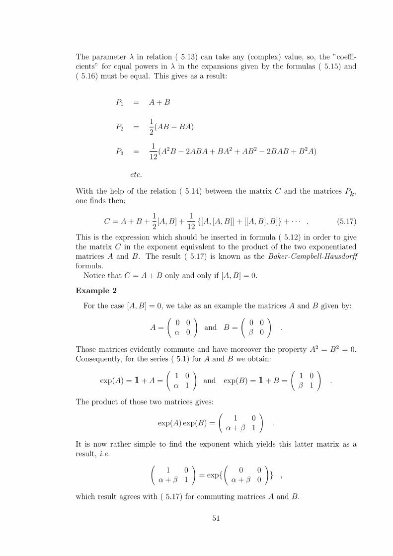
The parameter λ in relation ( 5.13) can take any (complex) value, so, the ”coeffi-cients” for equal powers in λ in the expansions given by the formulas ( 5.15) and( 5.16) must be equal. This gives as a result:
P1 = A+B
P2 =1
2(AB −BA)
P3 =1
12(A2B − 2ABA+BA2 + AB2 − 2BAB +B2A)
etc.
With the help of the relation ( 5.14) between the matrix C and the matrices Pk ,one finds then:
C = A+B +1
2[A,B] +
1
12[A, [A,B]] + [[A,B], B]+ · · · . (5.17)
This is the expression which should be inserted in formula ( 5.12) in order to givethe matrix C in the exponent equivalent to the product of the two exponentiatedmatrices A and B. The result ( 5.17) is known as the Baker-Campbell-Hausdorff
formula.Notice that C = A+B only and only if [A,B] = 0.
Example 2
For the case [A,B] = 0, we take as an example the matrices A and B given by:
A =
(
0 0α 0
)
and B =
(
0 0β 0
)
.
Those matrices evidently commute and have moreover the property A2 = B2 = 0.Consequently, for the series ( 5.1) for A and B we obtain:
exp(A) = 1+ A =
(
1 0α 1
)
and exp(B) = 1 +B =
(
1 0β 1
)
.
The product of those two matrices gives:
exp(A) exp(B) =
(
1 0α + β 1
)
.
It is now rather simple to find the exponent which yields this latter matrix as aresult, i.e.
(
1 0α+ β 1
)
= exp(
0 0α + β 0
)
,
which result agrees with ( 5.17) for commuting matrices A and B.
51

Example 3
For the case [A,B] 6= 0, we take as an example the matrices A and B given by:
A =
(
0 0α 0
)
and B =
(
0 β0 0
)
.
Using the results of the previous example 2, we find for the product of the exponentsof those two matrices the following result:
exp(A) exp(B) =
(
1 0α 1
)(
1 β0 1
)
=
(
1 βα 1 + αβ
)
.
In order to find the matrix C which exponentiated yields as a result the latter matrix,we follow the receipt of formula ( 5.17). Let us first collect the various ingredientsof this formula, i.e.
[A,B] = αβ
(
−1 00 1
)
,
[A, [A,B]] = −2α2β
(
0 01 0
)
,
[[A,B], B] = −2αβ2
(
0 10 0
)
, . . .
In the following expansion we will only take into account terms up to the third orderin α and β. Using formula ( 5.17), one obtains for the matrix C the result:
C =
−12αβ + · · · β − 1
6αβ2 + · · ·
α− 16α2β + · · · 1
2αβ + · · ·
.
Next, we determine the higher order powers of C as far as terms up to the thirdorder in α and β are involved, i.e.
C2 =
αβ + · · · 0 + · · ·
0 + · · · αβ + · · ·
, C3 =
0 + · · · αβ2 + · · ·
α2β + · · · 0 + · · ·
, . . .
When we put the pieces together, then we obtain the result:
exp(C) = 1+ C +1
2C2 +
1
6C3 + · · ·
=
(
1 00 1
)
+
−12αβ + · · · β − 1
6αβ2 + · · ·
α− 16α2β + · · · 1
2αβ + · · ·
+
+1
2
αβ + · · · 0 + · · ·
0 + · · · αβ + · · ·
+
1
6
0 + · · · αβ2 + · · ·
α2β + · · · 0 + · · ·
+ · · ·
=
(
1 βα 1 + αβ
)
+ higher order terms.
52

So, we have shown that the terms in α2β and αβ2 vanish in the sum of all termsin the series of exp(C). When one continues the expansion, the higher order termsalso cancel. Consequently, the complete result yields:
exp(C) =
(
1 βα 1 + αβ
)
.
However, the matrix C is a rather complicated expression, even for this simpleexample.
5.3 Orthogonal transformations.
Let us consider an orthogonal coordinate system S in n dimensions characterized bycoordinates xi (i = 1, . . . , n) and by the orthonormal basis vectors ei (i = 1, . . . , n).And let us furthermore consider in the same n-dimensional space a different orthog-onal coordinate system S ′ characterized by coordinates x′i (i = 1, . . . , n) and by theorthonormal basis vectors e′i (i = 1, . . . , n). The orthonormality of the basis vectorsis expressed by:
ei · ej = δij and e′i · e′j = δij (5.18)
The basis vectors of S and S ′ are related via linear transformation rules, givenby:
e′j = Rij ei and ej = (R−1)ij e′i. (5.19)
Using the orthonormality relations ( 5.18), we find for the matrix elements Rijof the transformation matrix R, the following property:
δij = e′i · e′j =
(
Rkiek
)
·(
Rljel
)
= RkiRlj ek · el
= RkiRljδkl = RkiRkj =(
RT)
ikRkj
=(
RTR)
ij,
or equivalently:
RTR = 1 or RT = R−1. (5.20)
Linear transformations for which the transposed of the matrix equals the inverseof the matrix, are said to be orthogonal. The determinant of such matrices equals±1, as can be seen from:
det(R)2 = det(R)det(R) = det(R)det(RT ) = det(RRT ) = det(1) = 1. (5.21)
Rotations are unimodular which means that they have determinant +1, anti-orthogonal transformations have determinant −1.
53

Rotations.
When the matrix M = exp(A) in ( 5.1) represents a rotation, then the matrix Ais traceless and anti-symmetric.
1. Traceless.
This is a direct consequence of the relations ( 5.11) and ( 5.21), i.e.
exp(Tr(A)) = det(M) = 1 = exp(0) consequently Tr(A) = 0 . (5.22)
2. Anti-symmetric.
The inverse of ( 5.1) is equal to M = exp(−A). This follows from the fact that Acommutes with −A and thus, according to formulas ( 5.12) and ( 5.17), one finds
exp(A) exp(−A) = exp(A− A) = 1 .
For the transposed MT of M , using
[A2]T = (AT )2 , [A3]T = (AT )3 , . . .
we obtain:
MT = exp(AT ) .
At this stage it is convenient to introduce a real parameter λ and define Mλ =exp(λA). Then also:
[Mλ]−1 = exp(−λA) and [Mλ]
T = exp(λAT ) . (5.23)
So, if Mλ is orthogonal, we find, expanding both expressions in the above formula( 5.23), the following equation:
1− λA+ · · · = [Mλ]−1 = [Mλ]
T = 1 + λAT + · · ·which is valid for arbitrary values of the real parameter λ and consequently yields
the solution AT = −A. In particular for λ = 1, we end up with:
[exp(A)]−1 = [exp(A)]T if and only if AT = −A . (5.24)
In example 1 (see formula 5.2) A is anti-symmetric and therefor M orthogonal.
5.4 Unitary transformations.
Complex n× n matrices M = exp(A) which satisfy the property:
M † =M−1 , (5.25)
are said to be unitary. Similar arguments as used above to show that for orthogonalmatrices M , A is anti-symmetric (i.e. formula 5.24), can be used here to show thatfor unitary matrices M , A is anti-Hermitean, i.e.
[exp(A)]−1 = [exp(A)]† if and only if A† = −A . (5.26)
54

5.5 The direct product of two matrices.
We will use the following definition for the direct product of two matrices: Let Arepresent an n1×n1 matrix and B an n2 ×n2 matrix, then for the direct product ofA and B we define:
A⊗ B =
A11B . . . A1n1B...
...
An11B . . . An1n1B
(5.27)
=
A11B11 . . . A11B1n2 A12B11 . . . . . . A1n1B1n2
......
......
A11Bn21 . . . A11Bn2n2 A12Bn21 . . . . . . A1n1Bn2n2
A21B11 . . . A21B1n2 A22B11 . . . . . . A2n1B1n2
......
......
An11Bn21 . . . An11Bn2n2 An12Bn21 . . . . . . An1n1Bn2n2
.
In terms of the matrix elements for the direct product of A and B, one mightalternatively define:
[A⊗ B](k − 1)n2 + i , (ℓ− 1)n2 + j = Akℓ Bij
k, ℓ = 1, . . . , n1
i, j = 1, . . . , n2
(5.28)
For the product of two such matrices one has the following expression:
(A⊗ B) (C ⊗ D) = (AC)⊗ (BD)
A, C n1 × n1 matrices
B,D n2 × n2 matrices(5.29)
proof:
We demonstrate below that identity ( 5.29) holds for an arbitrary matrix element,using definition ( 5.27) for the direct product of two matrices, or, alternatively,definition ( 5.28) for the matrix elements of a direct product:
[(A⊗ B) (C ⊗ D)](a− 1)n2 + b , (c− 1)n2 + d =
=n1n2∑
n = 1[A⊗ B](a− 1)n2 + b , n [C ⊗ D]n , (c− 1)n2 + d
55

=n1∑
k = 1
n2∑
i = 1[A⊗ B](a− 1)n2 + b , (k − 1)n2 + i
[C ⊗ D](k − 1)n2 + i , (c− 1)n2 + d
=n1∑
k = 1
n2∑
i = 1AakBbiCkcDid
=
n1∑
k = 1AakCkc
n2∑
i = 1BbiDid
= [AC]ac [BD]bd = [(AC)⊗ (BD)](a− 1)n2 + b , (c− 1)n2 + d .
Similarly, one may for the inverse of a direct product matrix show that:
[(A⊗ B)]−1 =(
A−1)
⊗(
B−1)
, (5.30)
assuming that 1⊗1 represents the identity matrix.
56

Chapter 6
The special orthogonal group intwo dimensions.
In this chapter we study the representations of the group of rotations in two dimen-sions. This group is the most easy example of a group which has an infinite numberof elements.
6.1 The group SO(2).
The special orthogonal group in two dimensions, SO(2), is defined by the set ofunimodular (i.e. with unit determinant), real and orthogonal 2× 2 matrices.In order to find the most general form of such matrices, let us assume that a, b,
c and d represent four real numbers which satisfy the property that ad − bc = 1.With those numbers we construct a 2× 2 matrix A, according to:
A =
(
a cb d
)
with det(A) = ad− bc = 1. (6.1)
When we assume that A is orthogonal, then A−1 = AT . This leads to the followingrelations for its components:
d = a and c = −b. (6.2)
Using also the condition ( 6.1) for the components of A, we find the following relationfor a and b:
a2 + b2 = 1 . (6.3)
Now, recalling that a and b are real numbers, we obtain as a consequence of thisrelation that:
−1 ≤ a ≤ +1 and − 1 ≤ b ≤ +1 . (6.4)
At this stage it is opportune to introduce a real parameter α such that:
a = cos(α) and b = sin(α) , (6.5)
in which case a and b satisfy simultaneously the conditions ( 6.3) and ( 6.4).
57

So, we obtain for a unimodular, real and orthogonal 2 × 2 matrix R(α), thefollowing general form:
R(α) =
(
cos(α) − sin(α)sin(α) cos(α)
)
for α ∈ (−π,+π] . (6.6)
When α takes values running from −π to +π, then one obtains all possible (infinitelymany!) unimodular, real and orthogonal 2× 2 matrices.
Next we must establish that the matrices ( 6.6) form a group:
1. Product.
Normal matrix multiplication defines a suitable group product for the set of ma-trices ( 6.6), i.e.
R(α2)R(α1) = R(α1 + α2). (6.7)
Strictly speaking might α1 + α2 be outside the parameter space (−π,+π] whenα1 and α2 are elements of this parameter space. But, we assume always an anglemodulus 2π if necessary.
2. Associativity.
Since matrix multiplication is associative, the above defined group product isautomatically endowed with the property of associativity.
3. Identity operator.
The identity operator, I, of the group product ( 6.7), which has the propertyIR(α) = R(α)I = R(α), is defined by the unit matrix:
I = R(α = 0) = 1 . (6.8)
4. Inverse.
For each group element R(α) exists an inverse group element R(−α) in SO(2),such that:
R(−α)R(α) = R(α)R(−α) = 1 . (6.9)
As a consequence of the above properties 1, 2, 3 and 4 we find that the specialorthogonal transformations in two dimensions, i.e. SO(2), form a group. This groupis moreover Abelian, because of the property ( 6.7), i.e.:
R(α2)R(α1) = R(α1 + α2) = R(α2 + α1) = R(α1)R(α2) . (6.10)
58

6.2 Irreps of SO(2).
Since SO(2) is an Abelian group, its irreps are one-dimensional. This propertyof Abelian groups has been shown for finite groups in ( 4.24). Consequently, therepresentation ( 6.6) of the group elements R(α) of SO(2) is reducible.Following the definition of a representation, the 2×2 matrices ( 6.6) might repre-
sent transformations D(R(α)) in a complex two-dimensional vector space. It is easyto verify that the unit vectors u1 and u−1, given by:
u1 =1√2
(
1i
)
and u−1 =1√2
(
i1
)
,
are eigenvectors of the matrices ( 6.6) for all values of α. The eigenvalues arerespectively given by:
c1(α) = e−iα and c−1(α) = e+iα .
So, at the one-dimensional subspace spanned by the unit vector u1, R(α) is rep-resented by the complex number exp(−iα), and at the one-dimensional subspacespanned by u−1, by exp(+iα). The similarity transformation which transforms thematrices D(R(α)) into a diagonal equivalent representation, is thus found to be:
1√2
(
1 −i−i 1
)
D(R(α))1√2
(
1 ii 1
)
=
(
exp(−iα) 00 exp(+iα)
)
.
The two resulting non-equivalent one-dimensional irreps of SO(2) are given by:
D(1)(R(α)) = exp(−iα) and D(−1)(R(α)) = exp(+iα) .
In the following we will simplify the notation for D and write D(α) instead ofD(R(α)). As we will see below, there are infinitely many non-equivalent irreps forSO(2).
An one-dimensional irrep is a set of linear transformations D(α); α ∈ (−π,+π]of a one-dimensional complex vector space V into itself, i.e.:
D(α) : V −→ V .
When u represents the only basis vector of V , then the transformation D(α) is fullycharacterized by:
D(α)u = c(α)u , for a complex number c(α) . (6.11)
Moreover, representations reflect the properties of the group. When, for example,for rotations yields the property:
[R(α)]n = R(nα) , n = 1, 2, . . .
then for the representation D(α) must yield the same property, i.e.:
[c(α)]n u = [D(α)]n u = D(nα)u = c(nα)u . (6.12)
59

The identity operator R(α = 0) is represented by the complex number 1, i.e.:
D(α = 0) = 1 . (6.13)
Next, let us study the possible representations for other values of α 6= 0. Let us forexample take α = 45. Using the relations ( 6.12) and ( 6.13), we obtain:
[c(π/4)]8 = c(2π) = c(0) = 1 .
Consequently, for R(π/4) one finds the following possible representations:
D(R(π/4)) = exp−ikπ/4 , k = 0,±1,±2, . . .
We may repeat this procedure for values of α of the form α = nπ/m (where |n| <m = 1, 2, . . . ), in order to find that for the representations of such transformationsone has the possibilities given by:
D(R(nπ/m)) = exp−iknπ/m , k = 0,±1,±2, . . .
Now, an arbitrary value for α can to any degree of accuracy be approximated byα = nπ/m for some integer numbers n and m > 0. Consequently, we are lead tothe conclusion that the possible representations for R(α) of SO(2) are given by:
D(R(α)) = exp−ikα , k = 0,±1,±2, . . . (6.14)
Each value of k gives an irrep which is not equivalent to any of the irreps for othervalues of k. This can easily be shown, since for any complex number s one has:
s−1 exp−ik1αs = exp−ik2α if and only if k1 = k2 .
Consequently, we may indicate the various one-dimensional vector spaces by anindex k in order to distinguish them, as well as the corresponding irrep, accordingto:
D(k)(α) : V (k) −→ V (k) .
We might moreover indicate the only basis vector of V (k) by uk, in order to obtain:
D(k)(α)uk = e−ikαuk , k = 0,±1,±2, . . . (6.15)
The representations D(k) are called the standard irreps of SO(2).
60

6.3 Active rotations in two dimensions.
An active rotation R(α) of a two-dimensional plane, over an angle α around theorigin of the coordinate system in the plane, is defined as the linear transformationof the plane into itself which rotates each vector of the plane over an angle α. Thecoordinate system though, remains in its place. The linear transformation R(α) isfully characterized once the images, ~u ′
1 and ~u ′2, are given of the vectors, ~u1 = e1
and ~u2 = e2, which originally are at the same positions as the two basis vectors ofthe coordinate system, i.e.:
~u ′1 = e1 cos(α) + e2 sin(α)
and
~u ′2 = −e1 sin(α) + e2 cos(α) . (6.16)
x
y
> P~r
x
y
···········
··········
····α
AA
AA
AAA
AAAAAAA
~r ′P ′
(a)
⇒R(α)
(b)
Figure 6.1: An active rotation of the plane: Physical objects are rotated aroundthe origin; the coordinate system remains in its place. Indicated are the situationsbefore (a) and after (b) the rotation R(α).
The image, ~w = w1e1 + w2e2, under the rotation R(α) of an arbitrary vector, ~v =v1e1 + v2e2, is then given by:
~w = v1~u′1 + v2~u
′2
= v1 cos(α)− v2 sin(α) e1 + v1 sin(α) + v2 cos(α) e2 ,
from which expression we deduce that the relation between the components (w1, w2)of the rotated vector and the components (v1, v2) of the original vector, is as follows:
(
w1
w2
)
=
(
cos(α) − sin(α)sin(α) cos(α)
)(
v1v2
)
= R(α)
(
v1v2
)
. (6.17)
61

Consequently, the active rotation R(α) is in the space of the components of two-dimensional vectors represented by the matrix ( 6.6). So, an active rotation in two
dimensions is a rotation of the position vectors of the plane with respect to a fixed
coordinate system. Equation ( 6.17) relates the components of the original vector tothe components of the rotated vector in the fixed basis.A possible way to concretize this transformation, is to imagine the x-axis and
the y-axis of the coordinate system to be drawn at your desk and a sheet of paper,representing the plane, on top of it. A certain point at the sheet of paper, indicatedby P in figure ( 6.1), is characterized by the position vector ~r before the rotationof the sheet. After rotating the sheet over an angle α around the origin, the samepoint at the sheet moves to a different position, indicated by P ′ in figure ( 6.1). Thepoint P ′ is characterized by the position vector ~r ′ = R(α)~r.Now, imagine the sheet of paper to be replaced by a sheet of metal which is heated
in one corner such that the temperature at the metal sheet is a function of position,say represented by the function T (~r). After rotating the sheet, its temperaturedistribution remains the same. However, in the new situation the function whichdescribes this distribution, is a different function of position, say T ′(~r). But, weassume that the rotation of the sheet does not change the temperature of a givenpoint P at the metal sheet. Consequently, one has the following relation betweenthe functions T and T ′:
T ′(R(α)~r) = T (~r) or equivalently T ′(~r) = T ([R(α)]−1~r) .
So, in function space (i.e. the space of functions f(~r) defined on the plane), theactive rotation R(α) induces the transformation:
R(α) : f −→ D(R(α))f , (6.18)
where D(R(α))f(~r) = f ′(~r) = f([R(α)]−1~r) .
6.4 Passive rotations in two dimensions.
A passive rotation R(α) of the plane is a rotation of the coordinate system of theplane. The vectors of the plane remain in their place, but the coordinate systemrotates over an angle indicated by α. The basis vectors, e′1 and e′2, of the newcoordinate system are related to the original basis vectors, e1 and e2, as follows:
e′1 = e1 cos(α) + e2 sin(α)
and
e′2 = −e1 sin(α) + e2 cos(α) . (6.19)
which is the same expression as given in formula ( 6.16), but with a completelydifferent meaning: In ( 6.16), the vectors ~u ′
1 and ~u ′2 represent the images of the
vectors which originally have the same positions as the basic vectors e1 and e2 ofthe fixed coordinate system. Here, e′1 and e′2 represent the basis vectors of the newcoordinate system.
62
A vector ~v can be characterized by its components (v1, v2) with respect to theoriginal basis vectors, as well as by its components (v′1, v
′2) in the new coordinate
system, i.e.:
~v = v1e1 + v2e2 = v′1e′1 + v′2e
′2 . (6.20)
The relation between (v1, v2) and (v′1, v′2), which can be found by substituting the
expressions ( 6.19) into formula ( 6.20), is given by:
v′1 = v1 cos(α) + v2 sin(α)
and
v′2 = −v1 sin(α) + v2 cos(α) ,
or, using formula ( 6.6), in a more compact notation:
(
v′1v′2
)
=
(
cos(α) sin(α)− sin(α) cos(α)
)(
v1v2
)
= [R(α)]−1
(
v1v2
)
. (6.21)
We find that in the case of a passive or coordinate transformation, the componentsv1 and v2, which describe the vector ~v in the original coordinate system, transformaccording to the inverse of the matrix R(α) into the components v′1 and v′2, whichdescribe the same vector ~v in the new coordinate system e′1 and e′2. Because of thisproperty, vectors are called contra-variant.
6.5 The standard irreps of SO(2).
From Fourier-analysis we know that the space of ”well-behaved” functions at theinterval (−π,+π] has as a basis the functions:
ψm(ϕ) = eimϕ , m = 0,±1,±2, . . . (6.22)
Any ”well-behaved” function f(ϕ) (ϕ ∈ (−π,+π]) can be expanded in a linearcombination of the basis (6.22), i.e.:
f(ϕ) =∞∑
m = −∞amψm(ϕ) , (6.23)
where the coefficients am are given by the innerproduct of the basis vector ψm withthe ”vector” f .The innerproduct of the orthonormal set of basis vectors ψm of this complex
vector space of ”well-behaved” functions at the interval (−π,+π], is defined by:
(ψm , ψn) =∫ +π
−πdϕ
2πψ⋆m(ϕ)ψn(ϕ) =
∫ +π
−πdϕ
2πei(n−m)ϕ = δmn . (6.24)
Consequently, the coefficients am of the expansion ( 6.23) are given by:
63

am = (ψm , f) =∫ +π
−πdϕ
2πψ⋆m(ϕ)f(ϕ) =
∫ +π
−πdϕ
2πf(ϕ)e−imϕ . (6.25)
At the Fourier basis ψm one might view the function f as an infinitely long columnvector with components am, i.e.
f =
...a−2
a−1
a0a1a2...
. (6.26)
In the following we study the effect of a passive rotation R(α) in the (x, y)-planeon the space of ”well-behaved” functions. The situation is shown in the figure ( 6.2)below.
x-e1
y
6e2
~r
P
ϕ···········································································
···········································································
x′
AAA
AA
AA
AAAAAAA
y′
*e′1AAAAK
e′2
~r
P
ϕ′α⇒
R(α)
Figure 6.2: A passive rotation of the plane: The coordinate system is rotated aroundthe origin; physical objects remain in their place.
Let us associate to each point at the unit circle in the plane a complex numbersuch that the resulting function is ”well-behaved”. In the coordinate system (e1, e2)this is described by a function a function f(ϕ) of the parameter ϕ. Whereas in thecoordinate system (e′1, e
′2) the same complex numbers are described by a function
f ′(ϕ′) of the angle ϕ′. Now, in a certain point P of the unit circle is the functionvalue independent of the choice of coordinates. Consequently, there exists a relationbetween f and f ′, given by:
f(ϕ) = f ′(ϕ′) = f ′(ϕ− α) . (6.27)
The Fourier basis at a given coordinate system is defined in formula ( 6.22). Therelevant variable is the azimuthal angle with respect to the basis vectors of thecoordinate system. Consequently, in the unprimed coordinate system are the valuesof the Fourier basis in the point P (see figure 6.2) determined by:
64

ψm(ϕ) = eimϕ , m = 0,±1,±2, . . .
and in the primed coordinate system by:
ψ′m(ϕ′) = eimϕ
′= eim(ϕ− α) , m = 0,±1,±2, . . .
So, we obtain the following relation between the two different Fourier bases:
ψ′m(ϕ′) = ψm(ϕ− α) .
This relation defines a representationD(F )(α) ofR(α) in the space of ”well-behaved”functions:
D(F )(α)ψm(ϕ) = ψ′m(ϕ′) = e−imαeimϕ = D(m)(α)ψm(ϕ) . (6.28)
In the vector space defined by vectors of the form ( 6.26), the representation
D(F )(α) of R(α) becomes a matrix representation. The matrix D(F )(α) might beviewed here as a diagonal matrix at the Fourier basis ψm, with diagonal elementsexp−imα, i.e.:
D(F )(α) =
. . .
e2iα 0
eiα
1
e−iα0 e−2iα
. . .
. (6.29)
In terms of the one-dimensional standard irreps defined in ( 6.15) the above matrixcan be written as:
D(F )(α) =
. . .
D(−2)(α) 0D(−1)(α)
D(0)(α)D(1)(α)
0 D(2)(α). . .
.
(6.30)
As a consequence we find that the representation D(F ) is completely reducible into
a direct sum the standard irreps D(m). For example, consider the one-dimensionalsubspace of ”well-behaved” functions, which have the form:
f(ϕ) = a1ψ1(ϕ),
65

where a1 may take any complex value. At this subspace is DF (α) given by:
DF (α)f(ϕ) = DF (α)
...000a10...
(ϕ) =
...000
D(1)(α)a10...
(ϕ) = D(1)(α))f(ϕ) . (6.31)
The Fourier components of the function f(ϕ) are given by am in the unprimedcoordinate system and by a′m in the primed system, i.e.:
f(ϕ) =∞∑
m = −∞amψm(ϕ) and f ′(ϕ′) =
∞∑
m = −∞a′mψ
′m(ϕ′) . (6.32)
So, using ( 6.27), ( 6.22) and ( 6.28), we obtain:
∞∑
m = −∞a′mψ
′m(ϕ′) = f ′(ϕ′) = f(ϕ) =
∞∑
m = −∞amψm(ϕ)
=∞∑
m = −∞ame
imϕ =∞∑
m = −∞ame
imαeim(ϕ− α)
=∞∑
m = −∞
(
ameimα
)
ψ′m(ϕ′) (6.33)
From which equality, using ( 6.29) and ( 6.30), we may conclude that:
a′m = ameimα =
[
D(F )(α)]−1
mmam . (6.34)
As a result, we find that in the case of a passive rotation R(α), the Fourier
basis transforms with D(F )(α) given in ( 6.29) and the Fourier components of a”well-behaved” function with the inverse of that matrix. It is in a way similar tothe transformation of the basis vectors of the coordinate system as given in formula( 6.19) in relation to the transformation of the components of a contra-variant vectoras shown in formula ( 6.21).
66

6.6 The generator of SO(2).
The group elements of SO(2) can be characterized by one parameter, the rotationangle; that is that all possible rotations in two dimensions are given by:
R(α) , −π < α ≤ +π. (6.35)
In the neighbourhood of the unit operation (α = 0), the above defined matricesform a one dimensional continuous matrix field. So, we might define the matrix Awhich is given by the derivative of the matrix field at α = 0, as follows:
A =d
dαR(α)
∣∣∣∣∣α = 0
=
(
0 −11 0
)
. (6.36)
The matrix A is called the generator of rotations in two dimensions. In thefollowing it will become clear why: For angles different from zero one has similarly:
d
dαR(α) =
(
− sin(α) − cos(α)cos(α) − sin(α)
)
=
(
0 −11 0
)(
cos(α) − sin(α)sin(α) cos(α)
)
= A R(α),
which differential equation can be solved by:
R(α) = expαA. (6.37)
The expansion of the exponent for the matrix A of formula ( 6.36) is shown in detailin ( 5.2) and it confirms the above equality.Because of the above representation of a rotation in terms of a parameter, α,
and the matrix A, it is that this matrix is called the generator of rotations in twodimensions.
A representation D(α) for the group elements R(α) of SO(2), can be translatedinto a representation d(A) of the generator A of the group, according to:
D(α) = expαd(A) . (6.38)
In the cae of the standard irreps ( 6.15) of SO(2), we find for the representations
d(k)(A) of the generator A of SO(2) the result:
d(k)(A) = −ik , k = 0,±1,±2, . . . (6.39)
6.7 A differential operator for the generator.
In the space of ”well-behaved” functions f(~r) = f(x, y) of the two real parameters xand y, we found in formula ( 6.18) the following representation for an active rotationR(α) of the parameter space (i.e. the (x, y)-plane):
D(α)f
(
~r =
(
xy
))
= f
(
[R(α)]−1
(
xy
))
. (6.40)
67

The lefthand side of this relation can be rewritten in terms of the correspondingrepresentation d(A) of the generator of SO(2), using the definition given in ( 6.38),i.e.:
D(α)f(~r) = expαd(A)f(~r) . (6.41)
Moreover, might the righthand side of equation ( 6.40) be expanded in a Taylorseries of the form:
f
(
~r +
(
∆x∆y
))
= f(~r) +
(
∆x∂
∂x+∆y
∂
∂y
)
f(~r) +
(6.42)
+1
2
(
(∆x)2∂2
∂x2+ 2∆x∆y
∂2
∂x∂y+ (∆y)2
∂2
∂y2
)
f(~r) + · · ·
Let us expand the series ( 6.41) and ( 6.42) in α. For ( 6.41) we obtain:
D(α)f(~r) = [1 + αd(A) +α2
2d(A)2 + · · ·]f(~r) . (6.43)
For ( 6.42) we need the expansions for ∆x and ∆y in α, i.e.:
(
∆x∆y
)
= R(−α)~r − ~r =
αy − α2
2 x+ · · ·
−αx− α2
2 y + · · ·
. (6.44)
Consequently, for ( 6.42) we obtain to first order in α, the following:
f([R(α)]−1~r) = f(~r) + α
(
y∂
∂x− x
∂
∂y
)
f(~r) . (6.45)
So, when we compare formula ( 6.43) with formula ( 6.45), then we find for therepresentation d(A) of the generator A of SO(2) in the space of ”well-behaved”functions f(x, y), to first order in α, the following differential operator:
d(A) = y∂
∂x− x
∂
∂y. (6.46)
Now, one might like to inspect the higher order terms in the expansions of theformulas ( 6.41) and ( 6.42). For ( 6.42), the second order in α term equals:
α2
2
(
−x ∂∂x
− y∂
∂y+ y2
∂2
∂x2− 2xy
∂2
∂x∂y+ x2
∂2
∂y2
)
f(~r) =α2
2
(
y∂
∂x− x
∂
∂y
)2
f(~r) .
(6.47)So, in comparing formula ( 6.43) with formula ( 6.47), we find that also to secondorder in α, the solution is given by the differential operator ( 6.46). In fact, thisresult is consistent with expansions up to any order in α.Moreover, when we introduce the azimuthal angle ϕ in the (x, y)-plane, according
to:
68
x = |~r| cos(ϕ) and y = |~r| sin(ϕ) ,
then we get for d(A), using formula ( 6.46), the differential operator given by:
d(A) = − ∂
∂ϕ. (6.48)
Because of this result, ∂/∂ϕ is sometimes refered to as the generator of rotations inthe (x, y)-plane.It is easy to demonstrate that relation ( 6.48) is the correct representation d(A)
in function space. The modulus of ~r remains invariant under a rotation, so the onlyrelevant variable of f(~r) is the azimuthal angle ϕ. Consequently, instead of formula( 6.40), one might take the more simple expression:
D(α)f(~r) = f(ϕ− α) = f(~r)− α∂
∂ϕf(~r) +
α2
2
(
∂
∂ϕ
)2
f(~r) + · · ·
Comparing this expansion with ( 6.43), we are unambiguously lead to the identifi-cation ( 6.48).
69

6.8 The generator for physicists.
Physicists prefer operators like x and −i∂/∂x. So, instead of the operator d(A) offormula ( 6.46), they prefer:
−ix ∂∂y
+ iy∂
∂x.
In order to suit that need, we take for the generator of SO(2) the operator L, definedby:
L = iA =
(
0 −ii 0
)
. (6.49)
The group elements R(α) of SO(2) can then be written in the form:
R(α) = exp−iαL . (6.50)
And, using the expressions ( 6.46) and ( 6.48), the representation d(L) of the gen-erator L turns out to be:
d(L) = −ix ∂∂y
+ iy∂
∂x= −i ∂
∂ϕ. (6.51)
Clearly, there exists no essential difference between the generator L and the genera-tor A. It is just a matter of taste. However, notice that whereas A of formula ( 6.36)is anti-symmetric, L of formula ( 6.49) is Hermitean. Both, A and L are traceless,since the group elements R(α) of SO(2) are unimodular (see formula 5.22).
In the case of the standard irreps ( 6.39), we find for the representations of d(k)(L)of the generator L the form:
d(k)(L) = k , k = 0,±1,±2, . . . (6.52)
6.9 The Lie-algebra.
The special orthogonal group in two dimensions, SO(2), is generated by the operatorL. This means that each element R(α) of the group can be written in the formR(α) = exp(−iαL). The reason that we only need one generator for the group SO(2)is the fact that all group elements R(α) can be parametrized by one parameter α,representing the rotation angle.Since α is a continuous parameter we may define the derivative of of the matrix
field R(α) with respect to α. When this derivative and all higher derivatives exist,then a group is called a Lie-group. SO(2) is a Lie-group.The operator L spans an algebra, which is a vector space endowed with a product.
A vector space is clear, because linear combinations, like α1L+α2L, generate groupelements, like R(α1 + α2). However the discussion on the precise details of theproduct will be postponed to the next chapter.Since this algebra generates a Lie-group it is called a Lie-algbra.
70

Chapter 7
The orthogonal group in twodimensions.
In this chapter we study the representations of the group of orthogonal transforma-tions in two dimensions. But, before doing so, let us first recapitulate what we havelearned so far.
7.1 Representations and the reduction procedure
Since, as we concluded from property ( 6.10) for its group elements, SO(2) is anAbelian group, its irreps are one-dimensional. This property of Abelian groups hasbeen shown for finite groups in ( 4.24). The arguments are, loosely speaking, asfollows:The equivalence classes of an Abelian group consist all of only one group element.
Hence, there are as many equivalence classes as group elements. Moreover, thenumber of non-equivalent irreducible representations of any group equals the numberof equivalence classes of the group. Consequently, in the case of an Abelian group onehas as many non-equivalent irreducible representations as there are group elementsin the group.Furthermore, one has that the sum of the square of the dimensions of the non-
equivalent irreducible representations also equals the number of group elements, asis shown in formula (4.10). This has for an Abelian group then as a consequencethat those dimensions can only be equal to one.
So, for any irreducible representation D(irrep), a group element R(α) of SO(2) isrepresented by a transformation of the complex numbers into the complex numbers,i.e.
D(irrep) (R(α)) : C −→ C . (7.1)
An arbitrary representation of SO(2) in a vector space of a higher dimension canbe reduced to one-dimensional irreducible representations at the basis of invariantone-dimensional subspaces. We have discussed the procedure for the defining rep-resentation of SO(2) in section ( 6.2) and for the space of complex functions of onevariable at the interval (−π,+π) at the Fourier basis in section ( 6.5), culminatingin formula ( 6.30).
71
7.2 The group O(2)
The orthogonal group in two dimensions, O(2), is defined by the set of real andorthogonal (i.e. A−1 = AT ) 2 × 2 matrices. For the determinant of such matricesone has the following relation
[det(A)]2 = det(A)det(A) = det(A)det(
AT)
= det(A)det(
A−1)
=
= det(
AA−1)
= det (1) = 1 ,
which leads to
det(A) = ±1 . (7.2)
For the unimodular, real and orthogonal 2 × 2 matrices, R(α), we found in section( 6.1) the general form
R(α) =
(
cos(α) − sin(α)sin(α) cos(α)
)
for α ∈ (−π,+π] . (7.3)
Those transformations of the two-dimensional plane onto itself are called proper
rotations.Following a similar reasoning as given in section ( 6.1), we find for the real and
orthogonal 2× 2 matrices with determinant −1, R(β), the general form
R(β) =
(
sin(β) cos(β)cos(β) − sin(β)
)
for β ∈ (−π,+π] . (7.4)
The latter type of matrices, which are referred to as the improper rotations, mightalso be written in the following form
R(β) = PR(β) with P =
(
0 11 0
)
. (7.5)
From expression ( 7.3) one learns moreover that the proper rotations form a sub-group of O(2), which is isomorphous to SO(2). Hence representations of O(2) arealso representations of SO(2). But this does not imply that irreducible represen-tations of O(2) are irreducible representations of SO(2). The latter statement caneasily be verified for the defining representation of O(2), given in formulas ( 7.3)and ( 7.4), since the unit vectors u1 and u−1, given by:
u1 =1√2
(
1i
)
and u−1 =1√2
(
i1
)
,
which are eigenvectors of the matrices ( 7.3) for all values of α, as discussed in section( 6.2), are not eigenvectors of the matrices ( 7.4). Consequently, the two-dimensionalvector space has no invariant subspaces under the defining representation of O(2),which representation is hence irreducible. However, its restriction to the subgroupSO(2) is reducible as we have seen in section ( 6.2).
72

The group product is conveniently studied once the square of the operation P ,defined in formula ( 7.5), is known and the product of R(α) and P is expressed interms of proper and improper rotations. Hence, we determine
P 2 = 1 and R(α)P =
(
− sin(α) cos(α)cos(α) sin(α)
)
= R(−α) . (7.6)
Using the definition ( 7.5) and the result ( 7.6), one may easily deduce that allpossible products of group elements of O(2) yield group elements of O(2), i.e.
(a) R(α)R(β) = R(α + β) ,
(b) R(α)R(β) = R(−α + β) ,
(c) R(α)R(β) = R(α + β) , and
(d) R(α)R(β) = R(−α + β) . (7.7)
The group structure follows from formula ( 7.7). In particular we find for the inversesof the two types of group elements
(a) [R(α)]−1 = R(−α) , and
(b)[
R(α)]−1
= R(α) . (7.8)
Furthermore, we obtain the following equivalence relations for proper and improperrotations.
(a) R(β)R(α)R(−β) = R(α) ,
(b) R(β)R(α)R(β) = R(−α) ,
(c) R(β)R(α)R(−β) = R(α− 2β) , and
(d) R(β)R(α)R(β) = R(−α + 2β) . (7.9)
From relations ( 7.9c and d) we conclude that all improper rotations are equivalentand from relation ( 7.9b) that all proper rotations are pairwise equivalent, exceptfor the unit element. Hence we obtain the following equivalence classes:
(type a) R(0) = 1 ,
(type b) R(α) , R(−α) , for each α ∈ (0,+π] , and
(type c)
R(β) , β ∈ (−π,+π]
. (7.10)
There is an infinity of type (b) equivalence classes, but half as many as groupelements in SO(2), which subgroup itself contains half as much group elements as
73

O(2), as can be seen from the construction given in formulas ( 7.3) and ( 7.4).The other two equivalence classes are related to the trivial and the almost trivialirreducible representations. Ignoring those two equivalence classes, we come to theconclusion that there are four times more group elements in O(2) than equivalenceclasses and hence than non-equivalent irreducible representations. As a consequenceall irreps of O(2) must be two-dimensional, with the exception of the two alreadymentioned. The defining representation of O(2), given in formulas ( 7.3) and ( 7.4),is an example of such representation.
7.3 Irreps of O(2).
An arbitrary representation, D, of O(2) has been defined in the foregoing as a setof unitary transformations of a vector space, V , into itself, i.e.
D(g) : V −→ V .
For the vector space V one might select the space of functions of one variable atthe interval (−π,+π), as in chapter ( 6). Now, in section ( 7.2) we have come tothe conclusion that D also forms a representation when restricted to the subgroupof proper rotations, which is isomorphous to SO(2), albeit possibly not irreducible.Moreover, in chapter ( 6) we have studied the irreducible representations of SO(2),hence we know that we may select a basis, . . . ψ−2, ψ−1, ψ0, ψ1, ψ2, . . ., in the vectorspace V at which the representation of a proper rotation, D (R(α)) acts as follows:
D (R(α))ψm = e−imαψm . (7.11)
Consequently, once the action of the representation of the improper rotation P ,defined in formula ( 7.5), is known, the whole representation is characterized. Forthat purpose we define
|ϕ〉 = D (P )ψm . (7.12)
We want to determine the relation of |ϕ〉 with the elements of the basis of the vectorspace V . Hence, also using formula ( 7.11), we do
D (R(α)) |ϕ〉 = D (R(α))D (P )ψm = D (R(α)P )ψm =
= D (PR(−α))ψm = D (P )D (R(−α))ψm =
= D (P ) eimαψm = eimαD (P )ψm = eimα|ϕ〉 ,
from which we conclude that |ϕ〉 is proportional to ψ−m, i.e.
D (P )ψm = |ϕ〉 = amψ−m . (7.13)
Notice that because of this result one has two-dimensional invariant subspaces ofthe vector space V which are spanned by the basis elements ψ−m and ψm, except
74

for the cases where m = 0. Consequently, when one organizes the basis of V in thefollowing order:
ψ0, ψ−1, ψ+1, ψ−2, ψ+2, ψ−3, ψ+3, . . . , (7.14)
then D(g) takes the form
D(g) =
D(0)(g)D(1)(g) 0
D(2)(g)0 D(3)(g)
. . .
, (7.15)
where D(0) is a number and where D(1), D(2), D(3), . . . are 2 × 2 matrices, for allelements g of SO(2).What is left now, is to figure out the value of the constant of proportionality am
of formula ( 7.13). First we settle that its absolute value must equal one, since wewant an unitary representation, i.e.
am = eiαm .
Next, also using formulas ( 7.6) and ( 7.13), we determine
ψm = 1ψm = D (1)ψm = D(
P 2)
ψm = D (P )D (P )ψm =
= D (P ) eiαmψ−m = eiαmD (P )ψ−m = eiαmeiα−mψm ,
from which we conclude that
α−m + αm = 0 , ±2π , ±4π , . . . . (7.16)
For m 6= 0 one might even get rid of the whole phase factor αm, by choosing anequivalent representation for which the new bases of the two-dimensional subspacesare given by
|m〉 = ψm and |−m〉 = eiαmψ−m , (7.17)
because then one has
D (P ) |m〉 = D (P )ψmeiαmψ−m = |−m〉
and D (P ) |−m〉 = D (P ) eiαmψ−m = eiαmeiα−mψm = |m〉 .
We thus find that, besides the two trivial representations, the irreducible rep-resentations of SO(2) are two-dimensional and characterized by positive integersm = 1, 2, 3, .... The representations of the proper and the improper rotations aregiven by
75

D(m) (R(α)) |m〉 = e−imα|m〉 ,
D(m) (R(α)) |−m〉 = eimα|−m〉 ,
D(m)(
R(β))
|m〉 = e−imβ |−m〉 ,
D(m)(
R(β))
|−m〉 = eimβ |m〉 . (7.18)
The two trivial irreducible representations are given by
D(1)(R) = D(1)(R) = 1 and D(1′)(R) = −D(1′)(R) = 1 . (7.19)
76
Chapter 8
The special orthogonal group inthree dimensions.
In this chapter we will study the group of special orthogonal 3× 3 matrices, SO(3).Those matrices represent rotations in three dimensions as we have seen in section( 5.3) at page 53.
8.1 The rotation group SO(3).
Similar to the group of rotations around the origin in two dimensions, we havethe group of rotations around the origin in three dimensions. An important dif-ference with rotations in two dimensions is that in three dimensions rotations donot commute. Consequently, the rotation group in three dimensions is not Abelian.The three rotations around the principal axes of the orthogonal coordinate system(x, y, z) are given by:
R(x, α) =
1 0 00 cos(α) − sin(α)0 sin(α) cos(α)
, R(y, ϑ) =
cos(ϑ) 0 sin(ϑ)0 1 0
− sin(ϑ) 0 cos(ϑ)
,
and R(z, ϕ) =
cos(ϕ) − sin(ϕ) 0sin(ϕ) cos(ϕ) 0
0 0 1
. (8.1)
Those matrices are unimodular (i.e. have unit determinant) and orthogonal.As an example that rotations in general do not commute, let us take a rotation
of 90 around the x-axis and a rotation of 90 around the y-axis. It is, using theabove definitions ( 8.1), easy to show that:
R(x, 90)R(y, 90) 6= R(y, 90)R(x, 90) . (8.2)
An arbitrary rotation can be characterized in various different ways. One way is asfollows: Let e1, e2 and e3 represent the orthonormal basis vectors of the coordinatesystem and let ~u1 = e1, ~u2 = e2 and ~u3 = e3 be three vectors in three dimensionswhich before the rotation R are at the positions of the three basis vectors. Theimages of the three vectors are after an active rotation R given by:
77

~u′i = R ~ui for i = 1, 2, 3.
The rotation matrix for R at the above defined basis ei (i = 1, 2, 3), consists thenof the components of those image vectors, i.e.
R =
(~u′1)1 (~u′2)1 (~u′3)1
(~u′1)2 (~u′2)2 (~u′3)2
(~u′1)3 (~u′2)3 (~u′3)3
. (8.3)
A second way to characterize a rotation is by means of its rotation axis, which isthe one-dimensional subspace of the three dimensional space which remains invariantunder the rotation, and by its rotation angle.In both cases are three free parameters involved: The direction of the rotation axis
in the second case, needs two parameters and the rotation angle gives the third. Inthe case of the rotation R of formula ( 8.3) we have nine different matrix elements.Now, if e1, e2 and e3 form a righthanded set of unit vectors, i.e. e1 × e2 = e3, thenconsequently form the rotated vectors ~u′1, ~u
′2 and ~u
′3 also a righthanded orthonormal
system, i.e. ~u′3 = ~u′1 × ~u′2. This leaves us with the six components of ~u′1 and ~u′2 asparameters. But there are three more conditions, |~u′1| = |~u′2| = 1 and ~u′1 · ~u′2 = 0.So, only three of the nine components of R are free.The matrix R of formula ( 8.3) is unimodular and orthogonal. In order to proof
those properties of R, we first introduce, for now and for later use, the Levi-Civitatensor ǫijk , given by:
ǫijk =
+1 for ijk = 123, 312 and 231.−1 for ijk = 132, 213 and 321.0 for all other combinations.
(8.4)
This tensor has the following properties:
(i) For symmetric permutations of the indices:
ǫjki = ǫkij = ǫijk. (8.5)
(ii) For antisymmetric permutations of indices:
ǫikj = ǫjik = ǫkji = −ǫijk. (8.6)
Now, using the definition of the Levi-Civita tensor and the fact that the rotatedvectors ~u′1, ~u
′2 and ~u′3 form a righthanded orthonormal system, we find for the de-
terminant of the rotation matrix R of formula ( 8.3) the following:
det(R) = ǫijkRi1Rj2Rk3 = ǫjik(~u′1)i(~u
′2)j(~u
′3)k
= (~u′1 × ~u′2)k(~u′3)k = ~u′3 · ~u′3 = 1 .
78

And for the transposed of the rotation matrix R we obtain moreover:(
RTR)
ij=(
RT)
ikRkj = RkiRkj = (~u′i)k(~u
′j)k = δij .
Consequently, the rotation matrix R is unimodular and orthogonal.
8.2 The Euler angles.
So, rotations in three dimensions are characterized by three parameters. Here weconsider the rotation which rotates a point ~a, defined by:
~a = (sin(ϑ) cos(ϕ), sin(ϑ) sin(ϕ), cos(ϑ)) , (8.7)
to the position ~b, defined by
~b = (sin(ϑ′) cos(ϕ′), sin(ϑ′) sin(ϕ′), cos(ϑ′)) . (8.8)
Notice that there exists various different rotations which perform this operation.Here, we just select one. Using the definitions ( 8.1), ( 8.7) and ( 8.8), it is not verydifficult to show that:
R(y,−ϑ)R(z,−ϕ)~a = z, R(z, ϕ′)R(y, ϑ′)z = ~b and R(y, ϑ′)R(y,−ϑ) = R(y, ϑ′−ϑ).
As a consequence of this results, we may conclude that a possible rotation whichtransforms ~a ( 8.7) into ~b ( 8.8), is given by:
R(ϕ′, ϑ′ − ϑ, ϕ) = R(z, ϕ′)R(y, ϑ′ − ϑ)R(z,−ϕ). (8.9)
This parametrization of an arbitrary rotation in three dimensions is due to Euler.The three independent angles ϕ′, ϑ′ − ϑ and ϕ are called the Euler angles.
8.3 The generators.
A second parametrization involves the generators of rotations in three dimensions,as, similar to the matrix A ( 6.36) for two dimensions, are called the following threematrices which result from the three basic rotations defined in ( 8.1):
A1 =d
dαR(x, α)
∣∣∣∣∣α = 0
=
0 0 00 0 −10 1 0
, A2 =
d
dϑR(y, ϑ)
∣∣∣∣∣ϑ = 0
=
0 0 10 0 0
−1 0 0
and A3 =d
dϕR(z, ϕ)
∣∣∣∣∣ϕ = 0
=
0 −1 01 0 00 0 0
. (8.10)
In terms of the Levi-Civita tensor, defined in formula ( 8.4), we can express thematrix representation ( 8.10) for the generators of SO(3), by:
(Ai)jk = −ǫijk. (8.11)
79

The introduction of the Levi-Civita tensor is very useful for the various derivationsin the following, since it allows a compact way of formulating matrix multiplications,as we will see. However, one more property of this tensor should be given here, i.e.the contraction of one index in the product of two Levi-Civita tensors:
ǫijkǫilm = ǫ1jkǫ1lm + ǫ
2jkǫ2lm + ǫ3jkǫ3lm
= δjlδkm − δjmδkl. (8.12)
Equiped with this knowledge, let us determine the commutator of two generators( 8.10), using the above properties ( 8.5), ( 8.6) and ( 8.12). First we concentrateon one matrix element ( 8.11) of the commutator:
[Ai, Aj ]kl = (AiAj)kl − (AjAi)kl = (Ai)km(Aj)ml − (Aj)km(Ai)ml
= ǫikmǫjml − ǫjkmǫiml = ǫmikǫmlj − ǫmjkǫmli
= δilδkj − δijδkl − (δjlδki − δjiδkl) = δilδkj − δjlδki
= ǫmijǫmlk = −ǫijmǫmkl = ǫijm(Am)kl
= (ǫijmAm)kl.
So, for the commutator of the generators ( 8.10) we find:
[Ai, Aj ] = ǫijmAm. (8.13)
Why commutation relations are important for the construction of representations ofLie-groups, will become clear in the following.
8.4 The rotation axis.
In order to determine a second parametrization of a rotation in three dimensions,we define an arbitrary vector ~n by:
~n = (n1, n2, n3), (8.14)
as well as its ”innerproduct” with the three generators ( 8.10), given by the expres-sion:
~n · ~A = niAi = n1A1 + n2A2 + n3A3. (8.15)
In the following we need the higher order powers of this ”innerproduct”. Actually,it is sufficient to determine the third power of ( 8.15), i.e.:
80

(~n · ~A)3 = (niAi)(njAj)(nkAk) = ninjnkAiAjAk.
We proceed by determining one matrix element of the resulting matrix. Using theabove property ( 8.12) of the Levi-Civita tensor, we find:
(~n · ~A)3ab = ninjnkAiAjAkab = ninjnk(Ai)ac(Aj)cd(Ak)db
= −ninjnkǫiacǫjcdǫkdb = −ninjnkδidδaj − δijδadǫkdb
= −ndnankǫkdb + n2nkǫkab = 0− n2nk(Ak)ab
= −n2~n · ~Aab.
The zero in the forelast step of the above derivation, comes from the deliberationthat using the antisymmetry property ( 8.6) of the Levi-Civita tensor, we have thefollowing result for the contraction of two indices with a symmetric expression:
ǫijknjnk = −ǫikjnjnk = −ǫikjnknj = −ǫijknjnk, (8.16)
where in the last step we used the fact that contracted indices are dummy and canconsequently be represented by any symbol.So, we have obtained for the third power of the ”innerproduct” ( 8.15) the follow-
ing:
(~n · ~A)3 = −n2~n · ~A. (8.17)
Using this relation repeatedly for the higher order powers of ~n · ~A, we may alsodetermine its exponential, i.e.
exp~n · ~A = 1+ ~n · ~A +1
2!(~n · ~A)2 + 1
3!(~n · ~A)3 + 1
4!(~n · ~A)4 + · · ·
= 1+ ~n · ~A +1
2!(~n · ~A)2 + 1
3!(−n2~n · ~A) + 1
4!(−n2(~n · ~A)2) + · · ·
= 1+ 1− n2
3!+n4
5!− n6
7!+ · · ·(~n · ~A) +
+ 12!
− n2
4!+n4
6!− n6
8!+ · · ·(~n · ~A)2
= 1+ n− n3
3!+n5
5!− n7
7!+ · · ·(n · ~A) +
+ n2
2!− n4
4!+n6
6!− n8
8!+ · · ·(n · ~A)2.
81

We recognize here the Taylor expansions for the cosine and sine functions. So,substituting these goniometric functions for their expansions, we obtain the followingresult:
exp~n · ~A = 1+ sin(n)(n · ~A) + (1− cos(n))(n · ~A)2. (8.18)
Next, we will show that this exponential operator leaves the vector ~n invariant.For that purpose we proof, using formula ( 8.16), the following:
(~n · ~A)~ni = (~n · ~A)ijnj = (nkAk)ijnj = nk(Ak)ijnj = −nkǫkijnj = 0,
or equivalently:
(~n · ~A)~n = 0. (8.19)
Consequently, the exponential operator ( 8.18) acting at the vector ~n, gives thefollowing result:
exp~n · ~A~n =[
1+ ~n · ~A+ · · ·]
~n = 1~n = ~n (8.20)
So, the exponential operator ( 8.18) leaves the vector ~n invariant and of course alsothe vectors a~n, where a represents an arbitrary real constant. Consequently, the axisthrough the vector ~n is invariant, which implies that it is the rotation axis whenthe exponential operator represents a rotation, i.e. when this operator representsan unimodular, orthogonal transformation. Now, the matrix ~n · ~A of formula ( 8.15)is explicitly given by:
~n · ~A =
0 −n3 n2
n3 0 −n1
−n2 n1 0
, (8.21)
which clearly is a traceless and anti-symmetric matrix. So, using the formulas( 5.22) and ( 5.24), we are lead to the conclusion that exp~n · ~A is orthogonal andunimodular and thus represents a rotation.In order to study the angle of rotation of the transformation ( 8.18), we introduce
a pair of vectors ~v and ~w in the plane perpendicular to the rotation axis ~n:
~v =
n2 − n3
n3 − n1
n1 − n2
and ~w = n× ~v = (n1 + n2 + n3)n− n
111
, (8.22)
where n is defined by n =√
n21 + n2
2 + n23.
The vectors ~v, ~w and ~n form an orthogonal set in three dimensions. Moreover,are the moduli of ~v and ~w equal.Using formula ( 8.21), one finds that under the matrix n · ~A the vectors ~v and ~w
transform according to:
(n · ~A)~v = ~w and (n · ~A)~w = −~v .
82
So, for the rotation exp(~n · ~A) of formula ( 8.18) one obtains for the vectors ~v and~w the following transformations:
~v ′ = exp(~n · ~A)~v = ~v + sin(n)~w + (1− cos(n))(−~v) = ~v cos(n) + ~w sin(n), and
~w ′ = exp(~n · ~A)~w = ~w + sin(n)(−~v) + (1− cos(n))(−~w) = −~v sin(n) + ~w cos(n).
The vectors ~v and ~w are rotated over an angle n in to the resulting vectors ~v ′ and~w ′. This rotation is moreover in the positive sense with respect to the direction ~nof the rotation axis, because of the choice ( 8.22) for ~w.Notice that the case n1 = n2 = n3, which is not covered by the choice ( 8.22), has
to be studied separately. This is left as an exercise for the reader.Concludingly, we may state that we found a second parametrization of a rotation
around the origin in three dimensions, i.e.:
R(n1, n2, n3) = exp~n · ~A, (8.23)
where the rotation angle is determined by:
n =√
n21 + n2
2 + n23,
and where the rotation axis is indicated by the direction of ~n.The vector ~n can take any direction and its modulus can take any value. Con-
sequently, exp(~n · ~A) may represent any rotation and so all possible unimodular,orthogonal 3× 3 matrices can be obtained by formula ( 8.18) once the appropriatevectors ~n are selected.
83

8.5 The Lie-algebra of SO(3).
Instead of the anti-symmetric generators An (n = 1, 2, 3) of formula ( 8.10), weprefer to continue with the Hermitean generators Ln = iAn (n = 1, 2, 3), which inexplicit form, using the expressions ( 8.10), can be given by:
L1 =
0 0 00 0 −i0 i 0
, L2 =
0 0 i0 0 0
−i 0 0
, and L3 =
0 −i 0i 0 00 0 0
. (8.24)
An arbitrary rotation R(n, α) with rotation angle α around the axis spanned byn, can, using formula ( 8.18), be expressed in terms of those generators, accordingto:
R(n, α) = exp−iαn · ~L = 1 + sin(α)(−in · ~L) + (1− cos(α))(−in · ~L)2. (8.25)
SO(3) is a Lie-group, because the derivatives ( 8.10) and all higher derivativesexist. The Lie-algebra is spanned either by A1, A2 and A3 or by −iL1, −iL2 and−iL3. The product of the Lie-algebra is given by the Lie-product, defined by thecommutator of two elements of the algebra. For the generators ( 8.24), using formula( 8.13), the Lie-products yield:
[Li, Lj ] = iǫijmLm. (8.26)
This establishes, moreover, their relation with the so-called angular momentumoperators in Quantum Mechanics.The generator space of SO(3) is an algebra. This implies that any real linear
combination of−iL1, −iL2 and−iL3 can serve as a generator of a rotation. However,the algebra may be extended as to include also complex linear combinations of thebasic generators. Those operators do in general not represent rotations, but mightbe very helpfull for the construction of representations of SO(3). Two such linearcombinations L+ and L− are given by:
L± = L1 ± iL2 . (8.27)
They satisfy the following commutation relations amongst themselves and with thethird generator L3:
[L3, L±] = ±L± and [L+, L−] = 2L3 . (8.28)
Notice moreover that, since L1 and L2 are Hermitean, the Hermitean conjugates ofL+ and L− satisfy:
L†+ = L− and L†
− = L+ . (8.29)
84

8.6 The Casimir operator of SO(3).
According to the first lemma of Schur ( 4.11), a matrix which commutes with allmatrices D(g) of an irreducible representation D for all elements of the group, mustbe proportional to the unit matrix. One irrep of SO(3) is formed by the rotationmatrices themselves. This will be shown in one of the next sections of this chapter.So, let us find a matrix which commutes with all rotation matrices. We representsuch matrix by its generator X , i.e. by exp(X). Then, since the matrix is supposedto commute with a rotation, we have:
exp(X) exp(−iαn · ~L) = exp(−iαn · ~L) exp(X) .
Now, when X commutes with n · ~L, then using the Baker-Campbell-Hausdorff for-mula ( 5.17), we find:
exp(X) exp(−iαn · ~L) = exp(X − iαn · ~L) = exp(−iαn · ~L) exp(X) .
Consequently, X must be an operator which commutes with all three generators L1,L2 and L3. A possible solution for such operator is given by:
X = ~L 2 = (L1)2 + (L2)
2 + (L3)2 , (8.30)
for which it is not difficult to prove that the following commutation relations hold:
[~L 2, Li] = 0 for i = 1, 2, 3 . (8.31)
The operator X , which is usually refered to as L2, is called the Casimir operator ofSO(3). Notice that L2 is not an element of the Lie-algebra, because it can not bewritten as a linear combination of generators. Nevertheless, Casimir operators areimportant for the classification of irreps of Lie-groups, as we will see in the following.For later use, we will give below some alternative expressions for L2 in terms of
the generator L3 and the generators L± of formula ( 8.27):
L2 = (L3)2 + L3 + L−L+
= (L3)2 − L3 + L+L−
= (L3)2 +
1
2
(
L+L− + L−L+)
. (8.32)
85

8.7 The (2ℓ + 1)-dimensional irrep d(ℓ).
A representation of the Lie-algebra of SO(3) and hence of the Lie-group itself, isfully characterized once the transformations d(ℓ)(Li) (for i = 1, 2, 3) of a certaincomplex vector space Vℓ onto itself are known. Let us select an orthonormal basisin Vℓ such that d(ℓ)(L3) is diagonal at that basis. From the considerations for SO(2)which lead to the formulas ( 6.39) and ( 6.52), we know that the eigenvalues for therepresentations of the generator L3 of rotations around the z-axis are integers. So,we might label the basis vectors of Vℓ according to their eigenvalues for d(ℓ)(L3), i.e.
d(ℓ)(L3) |ℓ,m >= m|ℓ,m > for m = 0,±1,±2, . . . (8.33)
The Casimir operator L2 for the representation, given by
L2 =[
d(ℓ)(L1)]2
+[
d(ℓ)(L2)]2
+[
d(ℓ)(L3)]2
, (8.34)
commutes with d(ℓ)(L1), d(ℓ)(L2) and d(ℓ)(L3). Consequently, for an irrep one has,
due the first lemma of Schur ( 4.11), that L2 equals a matrix proportional to theunit matrix. Let us take for the constant of proportionality the symbol λ, i.e.
L2 |ℓ,m >= λ|ℓ,m > for all basis vectors. (8.35)
In the following we will show that λ = ℓ(ℓ + 1) and that m runs from −ℓ to +ℓ.First, we proof that
m2 ≤ λ , (8.36)
from which we conclude that there must exist a maximum and a minimum value forthe integers m. Then we demonstrate that the representation of the operator L+ inVℓ transforms a basis vector |ℓ,m > in to a vector proportional to the basis vector|ℓ,m+ 1 > and similarly, the representation of the operator L− in Vℓ transforms abasis vector |ℓ,m > in to a vector proportional to the basis vector |ℓ,m− 1 >, i.e.
d(ℓ)(L±) |ℓ,m >= C±(ℓ,m)|ℓ,m± 1 > , (8.37)
where the coefficients C±(ℓ,m) represent the constants of proportionality. Becauseof the property ( 8.37) the operator L+ is called the raising operator of SO(3)and similarly L− the lowering operator. Property ( 8.37) leads us to conclude thatoperating on the basis vector which has the maximum eigenvalue mmax for d(ℓ)(L3),the raising operator must yield zero, and similarly on the basis vector with theminimum eigenvalue mmin, the lowering operator must yield zero.
d(ℓ)(L+)|ℓ,mmax >= d(ℓ)(L−)|ℓ,mmin >= 0 . (8.38)
Finally, we show that mmin = −mmax and introduce the symbol ℓ for the maximumvalue of m.The basis |ℓ,m > is orthonormal, which can be expressed by:
< ℓ,m|ℓ,m′ >= δmm′ . (8.39)
86

Relations which hold for the generators, also hold for the representations of thegenerators. So, using ( 8.29) and ( 8.32) we find:
L2 −[
d(ℓ)(L3)]2
=1
2
[d(ℓ)(L+)]†d(ℓ)(L+) + [d(ℓ)(L−)]†d(ℓ)(L−)
.
This leads, at the basis defined in formula ( 8.39), to the following property of thematrix elements for those operators:
λ−m2 = < ℓ,m|
L2 −[
d(ℓ)(L3)]2
|ℓ,m >
= < ℓ,m|12
[d(ℓ)(L+)]†d(ℓ)(L+) + [d(ℓ)(L−)]†d(ℓ)(L−)
|ℓ,m >
=1
2
∣∣∣d(ℓ)(L+)|ℓ,m >
∣∣∣
2+∣∣∣d(ℓ)(L−)|ℓ,m >
∣∣∣
2
≥ 0 .
This proofs relation ( 8.36) and leads to the introduction of a maximum eigenvaluemmax of d(ℓ)(L3) as well as a minimum eigenvalue mmin.Using the commutation relations ( 8.28), one obtains:
d(ℓ)(L3)d(ℓ)(L±) = d(ℓ)(L±L3 + [L3, L±]) = d(ℓ)(L±)d(ℓ)(L3)± d(ℓ)(L±) .
Acting with this operator on the basis ( 8.39), also using ( 8.33), one finds:
d(ℓ)(L3)
d(ℓ)(L±)|ℓ,m >
= d(ℓ)(L±)
d(ℓ)(L3)± 1
|ℓ,m >
= (m± 1)
d(ℓ)(L±)|ℓ,m >
. (8.40)
Consequently, one may conclude that d(ℓ)(L+)|ℓ,m > is proportional to the eigen-vector of d(ℓ)(L3) with eigenvalue m + 1, i.e. |ℓ,m + 1 >, and similarly that thevector d(ℓ)(L−)|ℓ,m > is proportional to |ℓ,m − 1 >. Yet another consequence of( 8.37) is that d(ℓ)(L+)|ℓ,mmax > vanishes, since |ℓ,mmax+1 > is not a basis vectorof Vℓ. Similarly, d(ℓ)(L−)|ℓ,mmin > vanishes. So, using the relations ( 8.32), onefinds:
0 = d(ℓ)(L−)d(ℓ)(L+)|ℓ,mmax >=(
L2 −[
d(ℓ)(L3)]2 − d(ℓ)(L3)
)
|ℓ,mmax >
= (λ− (mmax)2 −mmax)|ℓ,mmax > ,
and
0 = d(ℓ)(L+)d(ℓ)(L−)|ℓ,mmin >=(
L2 −[
d(ℓ)(L3)]2
+ d(ℓ)(L3))
|ℓ,mmin >
= (λ− (mmin)2 +mmin)|ℓ,mmin > ,
87

which leads to the identification mmin = −mmax and after defining ℓ = mmax, to theequation:
λ = ℓ2 + ℓ = ℓ(ℓ+ 1) . (8.41)
This way we obtain for Vℓ the following (2ℓ+ 1)-dimensional basis:
|ℓ,−ℓ >, |ℓ,−ℓ+ 1 >, . . . , |ℓ, ℓ− 1 >, |ℓ,+ℓ > . (8.42)
At this basis L3 is represented by a diagonal (2ℓ + 1)× (2ℓ + 1) matrix, which hasthe following form:
d(ℓ)(L3) =
−ℓ−ℓ + 1 0
. . .
0 ℓ− 1+ℓ
. (8.43)
Notice that d(ℓ)(L3) is traceless and Hermitean.The non-negative integer ℓ characterizes the irrep d(ℓ) of SO(3). To each possible
value for ℓ corresponds one non-equivalent unitary irrep. Its dimension is determinedby the structure of the basis ( 8.42), i.e.
dim(d(ℓ)) = 2ℓ+ 1 . (8.44)
The operator which characterizes the irrep, is the Casimir operator L2, defined informula ( 8.30). Its eigenvalues for any vector of Vℓ have the same value, equal toℓ(ℓ + 1). The basis ( 8.42) is chosen such that the generator L3 is represented bythe diagonal matrix given in ( 8.43).Because of the commutation relations ( 8.29), the operators L± defined in ( 8.27)
serve as raising and lowering operators, usefull to construct the whole basis of Vℓout of one single basis vector.Using equation ( 8.41) and once more the relations ( 8.29) and ( 8.32), we obtain
for the constants of proportionality of formula ( 8.37), moreover:
ℓ(ℓ+ 1)−m(m± 1) = < ℓ,m|
L2 −([
d(ℓ)(L3)]2 ± d(ℓ)(L3)
)
|ℓ,m >
= < ℓ,m|[
d(ℓ)(L±)]†d(ℓ)(L±)|ℓ,m >
=∣∣∣d(ℓ)(L±)|ℓ,m >
∣∣∣
2=∣∣∣C±(ℓ,m)
∣∣∣
2.
It is convention not to consider a phase factor for the coefficients C±(ℓ,m) and totake the following real solutions:
C±(ℓ,m) =√
ℓ(ℓ+ 1)−m(m± 1) . (8.45)
88

8.8 The three dimensional irrep for ℓ = 1.
As an example, let us study the three dimensional irrep d(1) of the Lie-algebra ofSO(3), at the basis of eigenstates of d(1)(L3) given by:
|1,−1 >=
100
, |1, 0 >=
010
and |1,−1 >=
001
. (8.46)
The matrix representation d(1)(L3) of L3 is, because of the above choice of basis,given by:
d(1)(L3) =
−1 0 00 0 00 0 +1
. (8.47)
The matrices d(1)(L±) at the basis ( 8.46) for the raising and lowering operators( 8.27) of SO(3) follow, using ( 8.45), from:
d(1)(L+)|1,−1 > =√2|1, 0 > , d(1)(L−)|1,−1 > = 0
d(1)(L+)|1, 0 > =√2|1,+1 > , d(1)(L−)|1, 0 > =
√2|1,−1 >
d(1)(L+)|1,+1 > = 0 , d(1)(L−)|1,+1 > =√2|1, 0 >
So, the matrices for the choice of basis ( 8.46) are given by:
d(1)(L+) =√2
0 0 01 0 00 1 0
and d(1)(L−) =
√2
0 1 00 0 10 0 0
. (8.48)
The matrices d(1)(L1) and d(1)(L2) can be obtained using the definition ( 8.27) for
the raising and lowering operators and the above result ( 8.48). This leads to:
d(1)(L1) =1√2
0 1 01 0 10 1 0
and d(1)(L2) =
1
i√2
0 −1 01 0 −10 1 0
. (8.49)
Now, we might also like to study the related representation D(1) of the group ele-ments of SO(3), in agreement with ( 8.25) given by:
D(1)(n, α) = exp−iαn · d(1)(~L) . (8.50)
Let us select the group elements shown in formula ( 8.1) and determine their rep-resentations for ℓ = 1. For a rotation around the x-axis, using formulas ( 8.25) and( 8.49), we find:
89

D(1) (R(x, α)) = exp−iαd(1)(L1)
= 1 + sin(α)(−id(1)(L1)) + (1− cos(α))(−id(1)(L1))2
=
12(cos(α) + 1) − i√
2sin(α) 1
2(cos(α)− 1)
− i√2sin(α) cos(α) − i√
2sin(α)
12(cos(α)− 1) − i√
2sin(α) 1
2(cos(α) + 1)
. (8.51)
Similarly, for a rotation around the y-axis, one obtains:
D(1) (R(y, ϑ)) = exp−iαd(1)(L2)
= 1+ sin(α)(−id(1)(L2)) + (1− cos(α))(−id(1)(L2))2
=
12(1 + cos(ϑ))
sin(ϑ)√2
12(1− cos(ϑ))
−sin(ϑ)√2
cos(ϑ)sin(ϑ)√
2
12(1− cos(ϑ)) −sin(ϑ)√
212(1 + cos(ϑ))
. (8.52)
And a rotation around the z-axis is here represented by:
D(1) (R(z, ϕ)) = exp−iαd(1)(L3)
= 1+ sin(α)(−id(1)(L3)) + (1− cos(α))(−id(1)(L3))2
=
eiϕ 0 0
0 1 0
0 0 e−iϕ
. (8.53)
The matrices ( 8.51), ( 8.52) and ( 8.53) of the three dimensional irreducible repre-sentation D(1) are not the same as the rotation matrices in three dimensions ( 8.1).However, one might notice that the traces are the same, respectively 2 cos(α) + 1,2 cos(ϑ) + 1 and 2 cos(ϕ) + 1. So, one might expect a similarity transformation Swhich brings the rotation matrices ( 8.1) at the above form. This is most conve-niently studied, using the expressions ( 8.24) for the generators and the expressions( 8.47) and ( 8.49). But this is left as an exercise for the reader.
90

8.9 The standard irreps of SO(3).
SO(3) is the symmetry group of the sphere in three dimensions. Points at the sphereare characterized by the polar angle ϑ and the azimuthal angle ϕ. As a basis forthe ”well-behaved” functions f(ϑ, ϕ) for the variables ϑ and ϕ, serve the spherical
harmonics:
Yℓm(ϑ, ϕ), for ℓ = 0, 1, 2, . . . and m = −ℓ, . . . ,+ℓ . (8.54)
The innerproduct for two functions χ and ψ in the space of functions on the sphereis defined as follows:
(ψ, χ) =∫
spheredΩ ψ∗(ϑ, ϕ)χ(ϑ, ϕ) . (8.55)
The spherical harmonics ( 8.54) form an orthonormal basis for this innerproduct,i.e.
∫
spheredΩ Y ∗
λµ(ϑ, ϕ)Yℓm(ϑ, ϕ) = δλℓδµm . (8.56)
Each function f(ϑ, ϕ) on the sphere can be expanded in terms of the sphericalharmonics, according to:
f(ϑ, ϕ) =∞∑
ℓ = 0
+ℓ∑
m = −ℓBℓmYℓm(ϑ, ϕ) . (8.57)
The coefficients Bℓm of the above expansion are, using the orthonormality relation( 8.56), given by:
Bℓm =∫
spheredΩ Y ∗
ℓm(ϑ, ϕ)f(ϑ, ϕ) . (8.58)
An active rotation R(n, α) in three dimensions induces a transformation in func-tion space (compare equation 6.18), given by:
D(n, α)f(~r) = f(
[R(n, α)]−1~r)
, (8.59)
where ~r indicates a point at the unit sphere, given by:
~r(ϑ, ϕ) =
sin(ϑ) cos(ϕ)sin(ϑ) sin(ϕ)
cos(ϑ)
. (8.60)
Let us study here the differential operators which follow for the three generatorsL1, L2 and L3, defined in formula ( 8.24), from the above equation. For a rotationR(z, α) around the z-axis we find, using formula ( 8.1), for ∆ϑ and ∆ϕ to first orderin α, the following:
~r(ϑ+∆ϑ, ϕ +∆ϕ) =
1 α 0−α 1 00 0 1
~r(ϑ, ϕ) =
sin(ϑ)cos(ϕ) + α sin(ϕ)sin(ϑ)−α cos(ϕ) + sin(ϕ)
cos(ϑ)
,
91

which is solved by:
∆ϑ = 0 and ∆ϕ = −α .
We obtain then for ( 8.59), expanding the lefthand side in terms of the representationof L3 and the righthand side in a Taylor series, both to first order in α, the following:
(1− iαd(L3)) f(~r) =
(
1− α∂
∂ϕ
)
f(~r) ,
from which we read the identification (compare also 6.51):
d(L3) = −i ∂∂ϕ
. (8.61)
For a rotation R(x, α) around the x-axis we find, once more using formula ( 8.1),for ∆ϑ and ∆ϕ to first order in α, the equations:
~r(ϑ+∆ϑ, ϕ +∆ϕ) =
1 0 00 1 α0 −α 1
~r(ϑ, ϕ) =
sin(ϑ) cos(ϕ)sin(ϑ) sin(ϕ) + α cos(ϑ)−α sin(ϑ) sin(ϕ) + cos(ϑ)
,
which are solved by:
∆ϑ = α sin(ϕ) and ∆ϕ = αcotg(ϑ) cos(ϕ) .
Insertion of those results in the righthand side of ( 8.59), leads to the identification:
d(L1) = i
sin(ϕ)∂
∂ϑ+ cotg(ϑ) cos(ϕ)
∂
∂ϕ
. (8.62)
For a rotation R(y, α) around the y-axis we find, again using formula ( 8.1), for∆ϑ and ∆ϕ to first order in α, the equations:
~r(ϑ+∆ϑ, ϕ+∆ϕ) =
1 0 −α0 1 0α 0 1
~r(ϑ, ϕ) =
sin(ϑ) cos(ϕ)− α cos(ϑ)sin(ϑ) sin(ϕ)
α sin(ϑ) cos(ϕ) + cos(ϑ)
,
which are solved by:
∆ϑ = −α cos(ϕ) and ∆ϕ = αcotg(ϑ) sin(ϕ) ,
and lead to the identification:
d(L2) = i
− cos(ϕ)∂
∂ϑ+ cotg(ϑ) sin(ϕ)
∂
∂ϕ
. (8.63)
The raising and lowering operators L± are, according to their definition ( 8.27),given by:
d(L±) = e±iϕ
icotg(ϑ)∂
∂ϕ± ∂
∂ϑ
. (8.64)
92

For the Casimir operator L2, using relation ( 8.30), we find the following differ-ential operator:
L2 = [d(L1)]2 + [d(L2)]
2 + [d(L3)]2
= −
∂2
∂ϑ2+ cotg(ϑ)
∂
∂ϑ+
1
sin2(ϑ)
∂2
∂ϕ2
= −
1
sin(ϑ)
∂
∂ϑsin(ϑ)
∂
∂ϑ+
1
sin2(ϑ)
∂2
∂ϕ2
(8.65)
The spherical harmonics Yℓm(ϑ, ϕ) for m = −ℓ, . . . ,+ℓ form the standard basisof a (2ℓ+ 1)-dimensional irrep in function space. For L3 their eigenvalues are givenby:
−i ∂∂ϕ
Yℓm(ϑ, ϕ) = d(L3)Yℓm(ϑ, ϕ) = mYℓm(ϑ, ϕ) . (8.66)
And for the Casimir operator L2, by:
−
1
sin(ϑ)
∂
∂ϑsin(ϑ)
∂
∂ϑ+
1
sin2(ϑ)
∂2
∂ϕ2
Yℓm(ϑ, ϕ) = L2Yℓm(ϑ, ϕ)
(8.67)
= ℓ(ℓ+ 1)Yℓm(ϑ, ϕ) .
93

8.10 The spherical harmonics.
Equation ( 8.66) is solved by:
Yℓm(ϑ, ϕ) = Xℓm(ϑ)eimϕ , (8.68)
where Xℓm(ϑ) is some yet unknown function of the polar angle ϑ. For m = 0equation ( 8.67) takes the following form:
− 1
sin(ϑ)
∂
∂ϑsin(ϑ)
∂
∂ϑXℓ0(ϑ) = ℓ(ℓ+ 1)Xℓ0(ϑ) .
By a change of variables:
ξ = cos(ϑ) and Pℓ(ξ) = Xℓ0(ϑ) , (8.69)
this differential equation transforms into:
− d
dξ(1− ξ2)
d
dξPℓ(ξ) = ℓ(ℓ+ 1)Pℓ(ξ) . (8.70)
This equation is known as Legendre’s differential equation, familiar in many problemsof mathematical physics. Its solutions are well-known. The first few solutions aregiven by the following Legendre polynomials:
P0(ξ) = 1 , P1(ξ) = ξP2(ξ) = 1
2(3ξ2 − 1) , and P3(ξ) = 1
2(5ξ3 − 3ξ)
(8.71)
For the construction of the spherical harmonics for m 6= 0, we may use the raisingand lowering operators, given in formula ( 8.64). Let us as an example, constructthe complete basis of spherical harmonics for the standard irrep corresponding toℓ = 1. For m = 0, using the expressions ( 8.68), ( 8.69) and ( 8.71), we find:
Y1,0(ϑ, ϕ) = N cos(ϑ) ,
where the normalization constant N is determined by relation ( 8.56), i.e.
1 = |N |2∫ 2π
0dϕ
∫ +1
−1d cos(ϑ) cos2(ϑ) = 4π|N |2/3 ,
leading to the conventional choice N =√
3/4π. For m = +1, using the formulas
( 8.48) and ( 8.64), we obtain:
√2 Y1,+1(ϑ, ϕ) = d(L+)Y1,0(ϑ, ϕ)
= e+iϕ
icotg(ϑ)∂
∂ϕ+
∂
∂ϑ
√
3
4πcos(ϑ)
= −√
3
4πe+iϕ sin(ϑ) ,
94

leading to the solution:
Y1,+1(ϑ, ϕ) = −√
3
8πe+iϕ sin(ϑ) .
For m = −1, also using the formulas ( 8.48) and ( 8.64), we obtain:
√2 Y1,−1(ϑ, ϕ) = d(L−)Y1,0(ϑ, ϕ)
= e−iϕ
icotg(ϑ)∂
∂ϕ− ∂
∂ϑ
√
3
4πcos(ϑ)
= +
√
3
4πe−iϕ sin(ϑ) ,
leading to the solution:
Y1,−1(ϑ, ϕ) = +
√
3
8πe−iϕ sin(ϑ) .
Applying once more the raising operator to the solution for m = +1, using formula( 8.64), we obtain moreover:
d(L+)Y1,+1(ϑ, ϕ) = e+iϕ
icotg(ϑ)∂
∂ϕ+
∂
∂ϑ
−√
3
8πe+iϕ sin(ϑ)
= −√
3
8πe+2iϕ −cotg(ϑ) sin(ϑ) + cos(ϑ) = 0 ,
which demonstrates that the series of basis elements terminates at m = +1 for theraising operator. Similarly for the lowering operator, one finds that the series ofbasis elements terminates at m = −1. So, the complete basis of the standard irrepof SO(3) for ℓ = 1, reads:
Y1,0(ϑ, ϕ) =
√
3
4πcos(ϑ) and Y1,±1(ϑ, ϕ) = ∓
√
3
8πe±iϕ sin(ϑ) .
95

8.11 Weight diagrams.
A weight diagram is a pictorial way to show the structure of the basis of an irrep. Itshows in diagrammatic form the eigenvalues of those generators of the group whichare represented by diagonal matrices. For an irrep of SO(3) the weight diagramconsists of one axis, along which the eigenvalues of the basis vectors of the irrep forthe generator L3 are indicated (in the case that the representation of L3 is diagonalat the basis of the irrep). In the figure below, the weight diagram for the irreduciblerepresentation of SO(3) corresponding to ℓ = 3 is depicted.
• • • • • • •-3 -2 -1 0 1 2 3
m--L+
L−
Figure 8.1: The weight diagram for d(3) of SO(3). The dots (•) at the horizontalline represent the basis vectors of the vector space V3. The values below the dotsrepresent their eigenvalues m for d(3)(L3).
The raising operator d(L+) takes steps of one unit in the positive direction of thehorizontal weight axis (see for example the weight diagram of figure 8.1), whenoperating on the basis vectors; the lowering operator d(L−), steps of one unit in thenegative direction.
8.12 Equivalence classes and characters.
In this section we discuss the relation which exists between the structure of rep-resentations for finite groups and the structure of the irreps of SO(3). For finitegroups we discovered that the number of inequivalent irreps equals the number ofequivalence classes of the group (see formula 4.23), which is intimately connected tothe structure of the character space for representations of finite groups (see formula4.17). So, let us begin by studying the equivalence classes of SO(3).
In order to do so, we first perform the following exercise: We determine, usingformula ( 8.21), the transformed matrix for (~n · ~A) under a rotation around thez-axis, for the following definition of the transformation:
~n ′ · ~A = R(z, α)(~n · ~A)R−1(z, α)
=
0 −n3 n1 sin(α) + n2 cos(α)
n3 0 −n1 cos(α) + n2 sin(α)
−n1 sin(α)− n2 cos(α) n1 cos(α)− n2 sin(α) 0
.
From this result we read for the transformed vector ~n ′ the relation:
96

~n ′ =
n1 cos(α)− n2 sin(α)
n1 sin(α) + n2 cos(α)
n3
= R(z, α)~n ,
which leads to the conclusion:
R(z, α)(~n · ~A)R−1(z, α) = R(z, α)~n · ~A . (8.72)
This result can be generalized to any rotation, not just rotations around the z-axis.In order to proof that, we need to mention a property of unimodular, orthogonalmatrices, i.e.
ǫℓmnRimRjn = ǫijkRkℓ .
Using this relation and formulas ( 5.20) and ( 8.11), we find:
[
R(~n · ~A)R−1]
ij=
= nk
[
RAkRT]
ij= nkRia(Ak)abRjb = nkRia(−ǫkab)Rjb
= = −nkǫijℓ)Rℓk = (R~n)ℓ(Aℓ)ij =[
(R~n) · ~A]
ij,
which proofs the validity of relation ( 8.72) for an arbitrary rotation R. Using theabove results, it is also not very difficult to proof that:
R exp~n · ~AR−1 = exp
(R~n) · ~A
.
Consequently, the group element exp~n · ~A in the above equation is equivalent
to the group element exp
(R~n) · ~A
(see the definition of equivalence in formula
1.23). The rotation angles are equal for both group elements, because the modulusof vector ~n does not change under a rotation, and therefore:
rotation angle of e(R~n) · ~A = |R~n| = |~n| = rotation angle of e~n · ~A .
Now, since R is arbitrary, we may conclude that all rotations which have the sameangle of rotation form an equivalence class. The trace of the rotation matrices outof one class can be determined by taking the trace of the rotation matrix of onerepresentant of the class. For example a rotation around the z-axis, which leads to:
Tr
e(R~n) · ~A
= Tr
e~n · ~A
= TrR(z, n) = 1 + 2 cos(n) .
All rotation matrices for group elements of the same equivalence class, have thesame character. Consequently, might one characterize the various classes of SO(3)
97

by the corresponding rotation angle. There are infinitely many angles and so, thereexist infinitely many equivalence classes in SO(3). Which settles moreover the pointthat there exist infinitely many irreps of SO(3).Also for a representation of SO(3) one might select the matrix representation of
rotations around the z-axis, in order to determine the characters for the variousequivalence classes. The representation of L3 is shown in formula ( 8.43). Theresulting representation for a rotation around the z-axis is therefore given by:
D(ℓ)(R(z, α)) = e−iαd(ℓ)(L3)
=
e+iℓα
e+i(ℓ− 1)α 0. . .
0 e−i(ℓ− 1)α
e−iℓα
.
So, its character is readily determined to be equal to:
χ(ℓ)(R(z, α)) =+ℓ∑
m = −ℓe−imα =
sin(
(2ℓ+ 1)α2
)
sin(α2
) .
For the particular case of the representation of the unit matrix R(z, 0), we havemoreover that its character yields the dimension of the representation, i.e.
dim(
d(ℓ))
= χ(ℓ)(R(z, 0)) =+ℓ∑
m = −ℓ1 = 2ℓ+ 1 ,
in agreement with ( 8.44).
98

Chapter 9
The special unitary group in twodimensions.
In this chapter we study the representations of the special unitary group in twodimensions, SU(2).
9.1 Unitary transformations in two dimensions.
Unitary 2 × 2 matrices form a group under normal matrix multiplication, becausethe product of two unitary matrices A and B is also unitary, i.e.
(AB)−1 = B−1A−1 = B†A† = (AB)† . (9.1)
The most general form of a unitary matrix in two dimensions is given by:
U(a, b) =
(
a∗ −b∗b a
)
, (9.2)
where a and b represent arbitrary complex numbers. When, moreover this matrixhas unit determinant, we have the condition:
|a|2 + |b|2 = 1 . (9.3)
A convenient paramatrization of unitary 2 × 2 matrices is by means of the Cayley-
Klein parameters ξ0, ξ1, ξ2 and ξ3, which is a set of four real parameters related tothe complex numbers a and b of formula ( 9.2) by:
a = ξ0 + iξ3 and b = ξ2 − iξ1 . (9.4)
When one substitutes a and b in formula ( 9.2) by the Cayley-Klein parameters,then one finds for a unitary 2× 2 matrix the expression:
U(ξ0, ~ξ) = ξ01− i~ξ · ~σ , (9.5)
where σ1, σ2 and σ3 represent the Hermitean Pauli matrices, defined by:
σ1 =
(
0 11 0
)
, σ2 =
(
0 −ii 0
)
and σ3 =
(
1 00 −1
)
. (9.6)
99

When, moreover the matrix ( 9.5) is unimodular, we have the condition:
(ξ0)2 + (ξ1)
2 + (ξ2)2 + (ξ3)
2 = 1 . (9.7)
This way we obtain three free parameters for the characterization of a 2 × 2 uni-modular and unitary matrix.Let us combine three parameters n1, n2 and n3 into a vector ~n given by:
~n =
n1
n2
n3
. (9.8)
By means of those parameters, one might select for the Cayley-Klein parameters( 9.4) which satisfy the condition ( 9.7), the following parametrization:
ξ0 = cos(n
2
)
and ~ξ = n sin(n
2
)
, (9.9)
where n and n are defined by:
n =
n1
n2
n3
=
1
n
n1
n2
n3
and n =
√
(n1)2 + (n2)2 + (n3)2 .
This way we find for an arbitrary unimodular unitary 2 × 2 matrix the followinggeneral expression:
U(~n) = 1 cos(n
2
)
− i(n · σ) sin(n
2
)
. (9.10)
Noticing moreover that (n ·~σ)2 =1, it is easy to show that U(~n) may also be writtenin the form:
U(~n) = exp
− i
2~n · ~σ
. (9.11)
The Pauli matrices ( 9.6) satisfy the following relations:For the product of two Pauli matrices one has:
σiσj = 1δij + iǫijkσk , (9.12)
for their commutator:
[
σi, σj
]
= 2iǫijkσk , (9.13)
and for their anti-commutator:
σi, σj
= σiσj + σjσi = 2δij1 (9.14)
100

9.2 The generators of SU(2).
The group of special unitary transformations in two dimensions SU(2) is a Lie-group. This can easily be understood if one considers the representation ( 9.10) foran arbitrary unimodular unitary transformation. Clearly, for that expression existthe partial derivatives with respect to its parameters to any order.According to formula ( 9.11) we may select for the generators of SU(2) the fol-
lowing set of 2× 2 matrices:
J1 =σ12
, J2 =σ22
and J3 =σ32
. (9.15)
The arbitrary special unitary transformation U(~n = αn) in two dimensions maythen, according to formula ( 9.11), be expressed by:
U(n, α) = e−iαn · ~J . (9.16)
The commutation relations for the generators ~J of SU(2) defined in formula( 9.15), can be read from the commutation relations ( 9.13), i.e.
[
Ji , Jj
]
= iǫijkJk . (9.17)
The commutation relations ( 9.17) for the generators ~J of SU(2) are identical to the
commutation relations ( 8.26) for the generators ~L of SO(3).Notice that, as in the case of SO(3), for SU(2) the generators ( 9.15) are traceless
and Hermitean.
9.3 The relation between SU(2) and SO(3).
In order to establish a relation between SU(2) and SO(3), we first study once morethe effect of a rotation R(n, α) in three dimensions on a vector ~x. A vector ~x maybe decomposed into a part parallel to the rotation axis n and a part perpendicularto this axis, as follows:
~x = (n · ~x)n + ~x− (n · ~x)n . (9.18)
The vector (n · ~x)n does not suffer any transformation under a rotation R(n, α)(see equation 8.20). But, the second part of ( 9.18), which represents a vector inthe plane perpendicular to the rotation axis, transforms into another vector in thatplane.For an orthonormal basis in this plane one might select the unit vectors v and w,
given by:
v =~x− (n · ~x)n√
~x 2 − (n · ~x)2and w =
n× ~x√
~x 2 − (n · ~x)2. (9.19)
The second part of ( 9.18) is before the transformation given by:
101

~x− (n · ~x)n = v√
~x 2 − (n · ~x) 2 .
And after the rotation over an angle α in the plane perpendicular to the rotationaxis n in the positive sense, by:
v cos(α) + w sin(α)√
~x 2 − (n · ~x)2 . (9.20)
So, using formulas ( 9.18), ( 9.19) and ( 9.20), we find for the transformed vector ~x ′
resulting from ~x under a rotation R(n, α), the following:
~x ′ = R(n, α)~x = ~x cos(α) + (n× ~x) sin(α) + (n · ~x)n(1− cos(α)) . (9.21)
A more elegant way to obtain the same result, is by means of the expression ( 8.18)for a rotation of an angle α around the axis indicated by n, i.e.
R(n, α) = eαn · ~A = 1+ sin(α)(n · ~A) + (1− cos(α))(n · ~A)2. (9.22)
Using formula ( 8.11) for the matrix elements of ~A, we find for (~n · ~A)~x the result:
[
(~n · ~A)~x]
i= nk(Ak)ijxj = −ǫkijnkxj = [~n× ~x]i . (9.23)
Moreover, using formula ( 8.12) for the contraction of two Levi-Civita tensors, we
obtain for (~n · ~A)2~x the expression:
[
(~n · ~A)2~x]
i= nanb(Aa)ij(Ab)jkxk = ǫaijǫbjknanbxk = (~n ·~x)ni−n2xi . (9.24)
Insertion of the result ( 9.23) and ( 9.24) in ( 9.22), yields once more the expression( 9.21) for R(n, α)~x.Having derived formula ( 9.21) for a rotation in three dimensions by two alterna-
tive methods, we return to the unitary transformations in two dimensions. Let usintroduce, by means of the Pauli matrices given in formula ( 9.6), a Hermitean 2×2matrix X defined by:
X = ~x · ~σ . (9.25)
The components of the vector ~x can, with the use of formula ( 9.14) for the anti-commutator of the Pauli matrices, uniquely be recovered from any Hermitean matrixX by taking the anti-commutator of X and ~σ, i.e.
~x = 12X,~σ = 1
2(X~σ + ~σX) . (9.26)
For an arbitrary unimodular unitary 2 × 2 matrix U(n, α), we define moreover thefollowing transformation for the matrix X :
X ′ = U(n, α)XU †(n, α) . (9.27)
Since U(n, α) is unitary and X Hermitean by definition ( 9.25), the matrix X ′ isalso Hermitean and thus by the procedure ( 9.26) uniquely related to a vector ~x ′.
102

Inserting the expressions ( 9.10) for U(n, α) and ( 9.25) for X , we obtain for thematrix X ′ the result:
X ′ =
1 cos(α
2
)
− i(n · σ) sin(α
2
)
(~x · ~σ)
1 cos(α
2
)
+ i(n · σ) sin(α
2
)
= (~x · ~σ) cos2(α
2
)
+ i [(~x · ~σ), (n · ~σ)] sin(α
2
)
cos(α
2
)
+
+ (n · ~σ)(~x · ~σ)(n · ~σ) sin2(α
2
)
. (9.28)
Using the relations ( 9.13) for the commutator of two Pauli-matrices and ( 9.12) fortheir product, it is easy to verify that:
i [(~x · ~σ), (n · ~σ)] = 2(n× ~x) · ~σ and
(n · ~σ)(~x · ~σ)(n · ~σ) = 2(n · ~x)(n · ~σ)− (~x · ~σ) .
Inserting those equations in ( 9.28), we find:
X ′ = (~x · ~σ) cos(α) + (n× ~x) · ~σ sin(α) + (n · ~x)(n · ~σ)(1− cos(α)) . (9.29)
The vector ~x ′ can be extracted from this matrix using the relation ( 9.26), for whichone obtains:
~x ′ = ~x cos(α) + (n× ~x) sin(α) + (n · ~x)n(1− cos(α)) .
Comparison of this result to the result of formula ( 9.21) for the expression of thevector ~x rotated around a rotation axis n by an angle α, leads us to the conclusionthat:
R(n, α)~x = 12
U(n, α)(~x · ~σ)U †(n, α) , ~σ
, (9.30)
which formula establishes the relation between a rotation in three dimensions and aunitary transformation in two dimensions.Notice however, that although for rotations one has:
R(n, α+ 2π) = R(n, α) ,
for unitary transformations in two dimensions, we have (see for example the expres-sion 9.10 for U(n, α)):
U(n, α+ 2π) 6= U(n, α) ! (9.31)
This implies that each rotation R(n, α) corresponds according to expression ( 9.30),to two different unitary transformations U(n, α) and U(n, α+ 2π).
103

9.4 The subgroup U(1).
The matrices U(z, α) form a subgroup U(1) of SU(2), because of the followingproperty:
U(z, α2)U(z, α1) = U(z, α1 + α2) . (9.32)
The explicit form of U(z, α), using relation ( 9.10), is given by:
U(z, α) =
e−i2α 0
0 e+i2α
. (9.33)
At the subspace spanned by the vector e1 =
(
10
)
, U(z, α), is represented by
exp−iα/2, according to:
U(z, α)ae1 = e−i2αae1 , so d(U(z, α)) = e−
i2α . (9.34)
The group U(1) is Abelian, as can be read from the property ( 9.32) for the matricesU(z, α). Consequently its irreps are one-dimensional (see also formula 4.24).Other one-dimensional irreps of U(z, α) may be given by:
d(U(z, α)) = e−imα . (9.35)
Now, since:
U(z, 2π) = −1 and U(z, 4π) = 1 , (9.36)
we have for the parameters m of formula ( 9.35), the condition that
e−im4π = 1 ,
which is solved by:
m = 0,±12,±1,±3
2,±2, . . . (9.37)
The representation ( 9.34) corresponds to the case m = 12.
104

9.5 The (2j + 1)-dimensional irrep 2j + 1.In section ( 9.2) we have seen that the generators ~J of SU(2) satisfy the same
commutation relations as the generators ~L of SO(3). Consequently, the structureof the Lie-algebras for the two groups is the same. Therefore, we can repeat theconstruction of irreps followed for SO(3). However, there is one important difference:In the case of SO(3), because of condition ( 8.33) for m, only odd values (2ℓ + 1)for the dimensions of its irreps are possible. For SU(2), because of the condition( 9.37), also even values (2j + 1) are possible for the dimensions of its irreps.The irreps of SU(2) are characterized by the parameter j, which, because of the
result ( 9.37), may take the values:
j = 0, 12, 1, 3
2, 2, . . . (9.38)
The (2j + 1)-dimensional irrep of the Lie-algebra of SU(2), d(j), is characterized bythe (2j + 1) orthonormal basis vectors, given by:
|j,+j > , |j, j − 1 > , . . . , |j,−j + 1 > , |j,−j > . (9.39)
The basis is chosen such that J3 is represented by a diagonal matrix, i.e.
d(j)(J3)|j,m >= m|j,m > . (9.40)
The raising and lowering operators J± are defined by the linear combinations of J1and J2 corresponding to those for L± in SO(3), i.e.
J± = J1 ± iJ2 . (9.41)
At the basis ( 9.39) for the (2j + 1)-dimensional irrep d(j) they are represented by:
d(j)(J±)|j,m >=√
j(j + 1)−m(m± 1)|j,m± 1 > . (9.42)
The Casimir operator, J2, defined by:
J2 =(
d(j)(J1))2
+(
d(j)(J2))2
+(
d(j)(J3))2
, (9.43)
has eigenvalues:
J2 |j,m >= j(j + 1)|j,m > . (9.44)
Besides allowing for more possible irreps, for SU(2) the representations have thesame structure as the representations of SO(3). In this chapter we use the symbol2j + 1, which indicates its dimension, for the irrep D(2j+1) of SU(2).
105

9.6 The two-dimensional irrep 2.For j = 1
2one has the two-dimensional irrep d(1/2) of the Lie-algebra of SU(2). We
denote the basis vectors by:
|12,+1
2>=
(
10
)
and |12,−1
2>=
(
01
)
(9.45)
The generator J3 is at this basis represented by a diagonal matrix. Its eigenvalues,as indicated by the notation for the basis vectors in formula ( 9.45), are respectively+1
2and −1
2. So, we find for d(1/2)(J3) the following matrix:
d(1/2)(J3) =12
(
+1 00 −1
)
=σ32
. (9.46)
For the raising and lowering operators we have, using formula ( 9.42), the transfor-mations:
d(1/2)(J+)|12,+1
2> =
√12(12+ 1)− 1
2(12+ 1)| > = 0 ,
d(1/2)(J+)|12,−1
2> =
√12(12+ 1) + 1
2(−1
2+ 1)|1
2,+1
2> = |1
2,+1
2> ,
d(1/2)(J−)|12,+1
2> =
√12(12+ 1)− 1
2(12− 1)|1
2,−1
2> = |1
2,−1
2> and
d(1/2)(J−)|12,−1
2> =
√12(12+ 1) + 1
2(−1
2− 1)| > = 0 .
(9.47)Consequently, the raising and lowering operators J± are here represented by thefollowing matrices:
d(1/2)(J+) =
(
0 10 0
)
= 12(σ1 + iσ2) and d(1/2)(J−) =
(
0 01 0
)
= 12(σ1 − iσ2) .
(9.48)This leads for the matrix representations of J1 and J2 furthermore to the result:
d(1/2)(J1) =σ12
and d(1/2)(J2) =σ22
. (9.49)
The Casimir operator J2, which is defined in formula ( 9.43), is for j = 12repre-
sented by 341, in agreement with:
J2|12, m >= 1
2(12+ 1)|1
2, m >= 3
4|12, m > . (9.50)
The matrices of the representation d(1/2) are exactly the same as the matrices ofthe definition of the Lie-algebra of SU(2).
106

9.7 The three-dimensional irrep 3.For j = 1 one has the three-dimensional irrep d(1) of SU(2). We denote the basisvectors by:
|1,+1 >=
100
, |1, 0 >=
010
and |1,−1 >=
001
(9.51)
The generator J3 is at this basis represented by a diagonal matrix. Its eigenvalues,as indicated by the notation for the basis vectors in formula ( 9.51), are respectively+1, 0 and −1. So, we find for d(1)(J3) the following matrix:
d(1)(J3) =
+1 0 00 0 00 0 −1
. (9.52)
For the raising and lowering operators we have at the basis ( 9.51), using formula( 9.42), the matrices:
d(1)(J+) =√2
0 1 00 0 10 0 0
and d(1)(J−) =
√2
0 0 01 0 00 1 0
. (9.53)
Notice that those matrices are not exactly equal to the corresponding matrix repre-sentations ( 8.48) of SO(3), because the choice of the basis ( 8.46) for SO(3) is notthe same as the above choice ( 9.51) for SU(2).The representation of the group elements U(n, α) of SU(2) is, according to the
relation ( 9.16), given by:
D(1)(U(n, α)) = e−iαn · d(1)( ~J) . (9.54)
For example for U(z, α), also using formula ( 9.52), one has:
D(1)(U(z, α)) =
e−iα 0 0
0 1 0
0 0 e+iα
. (9.55)
Now, the group elements U(z, α) and U(z, α + 2π) are not equal, but their matrixrepresentations as given in the above formula ( 9.55), are equal. The representationD(1) is therefore not faithfull. This is true for all odd dimensions. The reason isthat there are allways two different group elements U(n, α) and U(n, α+ 2π) whichcorrespond to one rotation R(n, α) (see formula 9.30) and that the odd dimensionalirreps are equivalent for SO(3) and SU(2).In order to determine the matrix representation of J2 we use the following relation
(see also formula 8.32):
J2 = (J3)2 + J3 + J−J+ . (9.56)
107

Using also the formulas ( 9.52) and ( 9.53), we find for the Casimir operator in thiscase:
J2 = 21 = 1(1 + 1)1 . (9.57)
9.8 The four-dimensional irrep 4.For j = 3
2one has the four-dimensional irrep d(3/2) of SU(2). We denote the basis
vectors by:
|32,+3
2>=
1000
, |3
2,+1
2>=
0100
, |3
2,−1
2>=
0010
and |32,−3
2>=
0001
.
(9.58)The generator J3 is at this basis represented by a diagonal matrix. Its eigenvalues,as indicated by the notation for the basis vectors in formula ( 9.58), are respectively+3
2, +1
2, −1
2and −3
2. So, we find for d(3/2)(J3) the following matrix:
d(3/2)(J3) =12
+3 0 0 00 +1 0 00 0 −1 00 0 0 −3
. (9.59)
For the raising and lowering operators we have at the basis ( 9.58), using formula( 9.42), the matrices:
d(3/2)(J+) =
0√3 0 0
0 0 2 0
0 0 0√3
0 0 0 0
and d(3/2)(J−) =
0 0 0 0√3 0 0 00 2 0 0
0 0√3 0
.
(9.60)Using the formulas (9.56), ( 9.52) and ( 9.53), we find for the Casimir operator inthis case:
J2 = 1541 = 3
2(32+ 1)1 . (9.61)
108

9.9 The product space 2 ⊗ 3.As an example of the representation of SU(2) in a product space, we select here theproduct space D(1/2) ⊗ D(1). The basis vectors of this space are, by means of thebasis vectors of the two bases ( 9.45) and ( 9.51), defined by:
|12,+1
2> ⊗|1, m >=
(
|1, m >0
)
and |12,−1
2> ⊗|1, m >=
(
0|1, m >
)
.
(9.62)Before we continue, for typographical reasons, we first simplify the notation of thebasis vectors to:
|m1 > |m2 >= |12, m1 > ⊗|1, m2 > . (9.63)
In a more explicit form one obtains for the basis defined in ( 9.62), column vectorsof length six, e1 , . . . , e6, where e1 represents a column vector which has only zeroesexcept for a 1 in the upper position, e2 represents a column vector which has onlyzeroes except for a 1 in the second position, etc., i.e.
|+ 12> |+ 1 >= e1 , |+ 1
2> | 0 >= e2 , |+ 1
2> | − 1 >= e3 ,
| − 12> |+ 1 >= e4 , | − 1
2> | 0 >= e5 and | − 1
2> | − 1 >= e6 .
(9.64)
Using the matrix representations D(1/2)(U(~n)) and D(1)(U(~n)) of a group elementU(~n) of SU(2) in the spaces respectively defined by the bases ( 9.45) and ( 9.51), welet U(~n) in the product space D(1/2) ⊗D(1) be represented by the following matrix:
D(U(~n)) =
[
D(1/2)(U(~n))]
11D(1)(U(~n))
[
D(1/2)(U(~n))]
12D(1)(U(~n))
[
D(1/2)(U(~n))]
21D(1)(U(~n))
[
D(1/2)(U(~n))]
22D(1)(U(~n))
.
(9.65)The above matrix represents a 6× 6 matrix, because D(1)(U(~n)) stands for a 3× 3matrix. The matrix ( 9.65) acts as follows at the basis vectors ( 9.62):
D(U(~n))|+ 12> |m >=
= D(U(~n))
(
|1, m >0
)
=
[
D(1/2)(U(~n))]
11D(1)(U(~n))|1, m >
[
D(1/2)(U(~n))]
12D(1)(U(~n))|1, m >
= D(1/2)(U(~n))
(
10
)
⊗D(1)(U(~n))|1, m >
=
D(1/2)(U(~n))|12,+1
2>
⊗
D(1)(U(~n))|1, m >
,
and similar:
109

D(U(~n))| − 12> |m >=
D(1/2)(U(~n))|12,−1
2>
⊗
D(1)(U(~n))|1, m >
. (9.66)
In terms of the generators (see formula 9.16), we have
e−i~n · d( ~J) = D(U(~n)) (9.67)
= D(1/2)(U(~n))⊗D(1)(U(~n)) = e−i~n · d(1/2)( ~J) ⊗ e−i~n · d(1)( ~J) ,
from which formula one deduces for the representation of the generators in theproduct space, the following:
d(Ji) = i
∂D(U(~n))
∂ni
∣∣∣∣∣~n = 0
= i
∂D(1/2)(U(~n))
∂ni
∣∣∣∣∣~n = 0
⊗D(1)(U(~n = 0)) +
+ iD(1/2)(U(~n = 0))⊗
∂D(1)(U(~n))
∂ni
∣∣∣∣∣~n = 0
= d(1/2)(Ji)⊗ 13×3 + 12×2 ⊗ d(1)(Ji) (9.68)
So, the representation d(O) in the product spaceD(1/2)⊗D(1) of an arbitrary elementO of the Lie-algebra of SU(2) is, using the irreps d(1/2) and d(1), given by the followingtransformation rule:
d(O)|m1 > |m2 >=
d(1/2)(O)|m1 >
|m2 > +|m1 >
d(1)(O)|m2 >
. (9.69)
• • • •−3/2 −1/2 1/2 3/2
m1 +m2-
| − 1
2> | − 1 > | − 1
2> | 0 >
|+ 1
2> | − 1 >
|+ 1
2> | 0 >
| − 1
2> |+ 1 >
|+ 1
2> |+ 1 >
Figure 9.1: The weight diagram for the product representation D(1/2) ⊗ D(1). Thedots at the horizontal line represent as indicated, the basis vectors ( 9.63) of theproduct vector space. The values below the dots represent their eigenvalues ford(J3).
At the basis ( 9.64) one obtains for J3 obviously a diagonal matrix, which is givenby:
d(J3)|m1 > |m2 >= (m1 +m2)|m1 > |m2 > . (9.70)
110

The weight diagram which results from formula ( 9.70) is depicted in figure ( 9.1).It does not have the form of a possible weight diagram for an irrep of SU(2), sincethere exist different eigenvectors of d(J3) with the same eigenvalue. Consequently,the representation of SU(2) in the product space D(1/2) ⊗ D(1) must be reducible.The principal issue of this section is therefore the reduction of the representation dinto irreps of SU(2).To that aim we first determine the matrix representation of J2 in the product
space, which for arbitrary representations neither is proportional to the unit matrix,nor diagonal. Diagonalization of the resulting matrix J2 leads to another basis ofthe product space, at which basis the matrix representations of the elements of theLie-algebra obtain the form shown in formula ( 2.34).We use the relation ( 9.56) for J2. The representation of J3 is, according to the
result ( 9.70), diagonal at the basis ( 9.62). So, d((J3)2) = [d(J3)]
2 is also diagonaland can be determined using formula ( 9.70). Consequently, what is left to becalculated for the representation of J2 as given by the expression ( 9.56), is theproduct of d(J−) and d(J+).At the basis ( 9.64), using the results ( 9.48) for d(1/2)(J−) and ( 9.53) for d(1)(J−),
one finds for d(J−) the following matrix:
d(J−) = d(1/2)(J−)⊗ 13×3 + 12×2 ⊗ d(1)(J−)
=
0 0
13×3 0
+
d(1)(J−) 0
0 d(1)(J−)
=
· · · · · ·√2 · · · · ··
√2 · · · ·
1 · · · · ·· 1 ·
√2 · ·
· · 1 ·√2 ·
, (9.71)
where the dots in the latter matrix represent zeroes.Let us verify one of the columns of the matrix obtained in formula ( 9.71). We
determine by means of the definition ( 9.69) for the representation of an arbitraryelement of the Lie-algebra of SU(2), the transformation of one of the basis vectors( 9.64):
d(J−)e2 = d(J−)|+ 12> | 0 >
= | − 12> | 0 > +
√2|+ 1
2> | − 1 >= e5 +
√2e3 .
The result corresponds to the second column of the matrix ( 9.71).For the representation of the raising operator J+ in the product spaceD(1/2)⊗D(1),
one finds similarly the transposed matrix:
111

d(J+) =
·√2 · 1 · ·
· ·√2 · 1 ·
· · · · · 1
· · · ·√2 ·
· · · · ·√2
· · · · · ·
. (9.72)
Next, one may determine the product of the matrices ( 9.71) and ( 9.72) and addthe result to the sum of the square of the matrix for d(J3) and the matrix for d(J3)itself, to find according to formula ( 9.56)for J2, the following matrix representationin the product space:
J2 =
154
· · · · ·· 11
4·
√2 · ·
· · 74
·√2 ·
·√2 · 7
4· ·
· ·√2 · 11
4·
· · · · · 154
. (9.73)
The resulting matrix is not even diagonal, let aside being proportional to the unitmatrix. In studying this matrix, one finds that out of the six basis vectors ( 9.64),two are eigenvectors of J2, i.e.
J2| ± 12> | ± 1 >= 15
4| ± 1
2> | ± 1 >= 3
2(32+ 1)| ± 1
2> | ± 1 > . (9.74)
The eigenvalues for d(J3) for those two vectors can be read from equation ( 9.70)to be equal to ±3
2, which leads us to conclude that the two basis vectors ( 9.74)
of the product space form also basis vectors of the irrep d(3/2) of SU(2) for j = 32.
Therefore we identify:
|32,±3
2>= | ± 1
2> | ± 1 > . (9.75)
Now, we might search for the other eigenvectors of J2 in order to obtain the re-maining basis vectors of the four dimensional irrep d(3/2) of SU(2) and the basisvectors of the other, yet unknown, irreps. But, there exists a more elegant method:Starting from one basis vector, one can construct the complete basis for an irrep byrepeatedly applying the raising or lowering operator.Let us start with the basis vector |3
2,+3
2> and apply the representation of the
lowering operator to it. For the lefthand side of equation ( 9.75) we find:
d(3/2)(J−)|32,+3
2>=
√32(32+ 1)− 3
2(32− 1)|3
2,+1
2>=
√3|3
2,+1
2> . (9.76)
And applying d(J−) to the righthand side of equation ( 9.75), one obtains:
d(J−)|+ 12> |+ 1 >= | − 1
2> |+ 1 > +
√2|+ 1
2> | 0 > . (9.77)
The results ( 9.76) and ( 9.77) lead to the identification:
112

|32,+1
2>=
√13| − 1
2> |+ 1 > +
√23|+ 1
2> | 0 > . (9.78)
The eigenvalue of d(J3) for the vector at the righthand side of this formula equals+1
2, since both terms in the linear combination have that eigenvalue for d(J3). Using
the matrix representation ( 9.73) for J2 in the product space and the identifications( 9.64), then we find that the righthand side of ( 9.78) is also an eigenvector of J2
with eigenvalue 154, as expected.
Applying next d(3/2)(J−) to the lefthand side of ( 9.78) and d(J−) to the righthandside, we come to the identification:
|32,−1
2>=
√23| − 1
2> | 0 > +
√13|+ 1
2> | − 1 > . (9.79)
So, with the above procedure we found the four basis vectors ( 9.75), ( 9.78) and( 9.79) of the four dimensional irrep 4 of SU(2) for j = 3
2.
At the subspace of the product space, which is spanned by the basis vectors whichhave eigenvalue +1
2for d(J3), i.e.
|12,+1
2> ⊗|1, 0 > and |1
2,−1
2> ⊗|1,+1 > .
we found one linear combination, ( 9.78), which is an eigenvector of J2. A possiblevector orthogonal to that linear combination is given by:
√13|12,+1
2> ⊗|1, 0 > −
√23|12,−1
2> ⊗|1,+1 > .
This vector is also an eigenvector of J2 with eigenvalue 34. Its eigenvalue for d(J3)
is evidently equal to +12. Consequently, we may identify:
|12,+1
2>=
√13|+ 1
2> | 0 > −
√23| − 1
2> |+ 1 > . (9.80)
Applying d(1/2)(J−) to the lefthand side and d(J−) to the righthand side, gives usthe other basis vector of the two-dimensional irrep d(1/2) of SU(2), i.e.
|12,−1
2>=
√23|+ 1
2> | − 1 > −
√13| − 1
2> | 0 > . (9.81)
When we perform a basis transformation in the product space from the old basis( 9.64) to a new basis given by the expressions ( 9.75), ( 9.78), ( 9.79), ( 9.80)and ( 9.81), then one obtains for the matrix representations of all elements of thealgebra and hence of the group, matrices of the form of a direct sum of a 4×4 matrixequivalent to the irrep d(3/2) and a 2 × 2 matrix equivalent to d(1/2). Consequently,the product space D(1/2) ⊗ D(1) yields a representation which is equivalent to thedirect sum of the four-dimensional and the two-dimensional irreps of SU(2).For example, when we select in the direct product space 2⊗3 the basis given
by:
e′1 = |+ 12> |+ 1 > ,
e′2 =√
13| − 1
2> |+ 1 > +
√23|+ 1
2> | 0 > ,
113

e′3 =√
23| − 1
2> | 0 > +
√13|+ 1
2> | − 1 > ,
(9.82)
e′4 = | − 12> | − 1 > ,
e′5 =√
13|+ 1
2> | 0 > −
√23| − 1
2> |+ 1 > and
e′6 =√
23|+ 1
2> | − 1 > −
√13| − 1
2> | 0 > ,
then we find for all matrices d′(O) which represent elements O of the Lie-algebra ofSU(2) at the new basis ( 9.82), the form:
d′(O) =
d(3/2)(O) 0
0 d(1/2)(O)
. (9.83)
For J2 we obtain at the new basis ( 9.82), the matrix representation given by:
J2 =
15414×4 0
0 3412×2
=
J2(j = 32) 0
0 J2(j = 12)
. (9.84)
For the matrix representations D′(U) at the basis ( 9.82) of all group elements U ofSU(2) we find, using the fact that the product of two matrices which have the form( 9.83) also has that form and hence the exponent exp−iO, the general expression:
D′(U) =
D(3/2)(U) 0
0 D(1/2)(U)
. (9.85)
This result may symbolically be represented by:
2 ⊗ 3 = 4 ⊕ 2 . (9.86)
114

9.10 Clebsch-Gordan or Wigner coefficients.
The identifications between the basis vectors ( 9.62) of the product space 2⊗ 3and the basis vectors of the irreps 4 and 2, involve the linear combinations givenin the formulas ( 9.75), ( 9.78), ( 9.79), ( 9.80) and ( 9.81). In general, let us for the
two irreps d(j1) and d(j2) consider the product space given by:
2j1 + 1 ⊗ 2j2 + 1 . (9.87)
Let moreover, in the reduction of the representation d in this product space, appear
the irrep d(j) of SU(2). The identification of a basis vector |j,m > with a linearcombination of basis vectors of the product space ( 9.87) can then be written as:
|j,m >=∑
m1, m2
Cj1 j2 j
m1 m2 m|j1, m1 > ⊗|j2, m2 > . (9.88)
The coefficients Cj1, j2, j;m1, m2, m in this linear combination are called Clebsch-
Gordan or Wigner coefficients.In formula ( 9.75) we find the following Clebsch-Gordan coefficients:
C12
1 32
+12
+1 +32
= 1 and C12
1 32
−12
−1 −32
= 1 ,
in formula ( 9.78)
C12
1 32
−12
+1 +12
=√
13
and C12
1 32
+12
0 +12
=√
23
,
in formula ( 9.79)
C12
1 32
−12
0 −12
=√
23
and C12
1 32
+12
−1 −12
=√
13
,
in formula ( 9.80)
C12
1 12
+12
0 +12
=√
13
and C12
1 12
−12
+1 +12
= −√
23
,
and in formula ( 9.81)
C12
1 12
+12
−1 −12
=√
23
and C12
1 12
−12
0 −12
= −√
13
,
From the construction it might be clear that the Clebsch-Gordan coefficient given byC(1
2, 1, 1
2; +1
2, 0,+1
2), which relates the various basis vectors given in formula ( 9.80),
could as well have been chosen negative and even complex. It is however conventionto choose one specific Clebsch-Gordan coefficient in each irrep d(j) which is containedin the direct product 2j1 + 1 ⊗ 2j2 + 1, according to the following condition:
115

Cj1 j2 j
j1 j − j1 jreal and positive. (9.89)
Notice that also the identification ( 9.75) implies the rather arbitrary, although themost obvious, choice C(1
2, 1, 3
2; +1
2,+1,+3
2) = +1, only at this stage explained by
the above condition.As a consequence of condition ( 9.89) are all Clebsch-Gordan coefficients real. In
that case is the matrix which describes the transformation from the orthonormal ba-sis of the product space to the orthonormal bases of the various irreps, orthogonal.The matrix elements of this matrix are the Clebsch-Gordan coefficients ( 9.88). Con-sequently, using the orthonormality conditions of rows and columns of an orthogonalmatrix, one obtains:
∑
m1, m2
Cj1 j2 j
m1 m2 mC
j1 j2 j′
m1 m2 m′ = δjj′δmm′
and
∑
j,mC
j1 j2 j
m1 m2 mC
j1 j2 j
m′1 m′
2 m= δm1m
′1δm2m
′2. (9.90)
Notice furthermore the following property of Clebsch-Gordan coefficients:
Cj1 j2 j
m1 m2 m= 0 for m1 +m2 6= m . (9.91)
However, it is not generally true that Clebsch-Gordan coefficients are nonzero ifm1 +m2 = m; for example:
C1 1 1
0 0 0= 0 .
Some of the most useful symmetry relations for the Clebsch-Gordan coefficients aresummarized by the equation:
Cj2 j1 j
m2 m1 m= (−1)j − j1 − j2C
j1 j2 j
m1 m2 m= C
j1 j2 j
−m1 −m2 −m . (9.92)
116

9.11 The Lie-algebra of SU(2).
The generator subspace of the Lie-algebra of SU(2) consists of purely imaginary
linear combinations of the basic generators ~J = ~σ/2. Linear combinations whichare not purely imaginary, like the raising and the lowering operators J±, do notrepresent generators of the group, but can be very useful for the construction andclassification of irreps. For SU(2), we define the following set of traceless standardmatrices Aij (i, j = 1, 2), by:
[
Aij
]
kℓ= δikδjℓ − 1
2δijδkℓ for i, j, k, ℓ = 1, 2. (9.93)
Their relation with the generators ~J is given by:
A11 = 12
(
+1 00 −1
)
= J3 , A12 =
(
0 10 0
)
= J+ ,
A21 =
(
0 01 0
)
= J− and A22 = 12
(
−1 00 +1
)
= −J3 .
(9.94)Using their definition ( 9.93) or alternatively the above explicit expressions, it iseasy to verify the following commutation relations for the standard matrices:
[
Aij, Akℓ
]
= δjkAiℓ − δiℓAkj . (9.95)
The Casimir operator J2 can, using the relations ( 8.32) and ( 9.94), be expressedin terms of the standard matrices, i.e.
J2 = (J3)2 + 1
2(J+J− + J−J+) = 1
2
(J3)2 + J+J− + J−J+ + (−J3)2
= 12AijAji . (9.96)
It is easy to show that this operator commutes with all standard matrices ( 9.93)and hence with all generators of SU(2). Using the commutation relations ( 9.95),we find:
2[
J2, Akℓ
]
=[
AijAji, Akℓ
]
= Aij
[
Aji, Akℓ
]
+[
Aij, Akℓ
]
Aji
= Aij(δikAjℓ − δjℓAki) + (δjkAiℓ − δiℓAkj)Aji = 0 . (9.97)
In general, one might, using the standard matrices ( 9.93), construct similar opera-tors which commute with all generators of SU(2). For example, it is straightforwardto demonstrate that the operator AijAjkAki commutes with all standard matrices
and so, could perfectly serve as a Casimir operator. However, one has, using thecommutation relations ( 8.28), the identity:
117

AijAjkAki = A11A11A11 + A11A12A21 + A12A21A11 + A12A22A21 +
+ A21A11A12 + A21A12A22 + A22A21A12 + A22A22A22
= (J3)3 + J3J+J− + J+J−J3 + J+(−J3)J− +
+ J−J3J+ + J−J+(−J3) + (−J3)J−J+ + (−J3)3
= J3[
J+, J−]
+[
J+, J−]
J3 + J+[
J−, J3]
+[
J−J3, J+]
= 2
(J3)2 + 1
2(J+J− + J−J+)
= AijAji . (9.98)
Consequently, no new Casimir operator results from the contraction of three stan-dard matrices.
9.12 The product space 2 ⊗ 2 ⊗ 2.At the basis ( 9.45) for the irrep D(1/2) of SU(2), the matrix representations of thegenerators and hence of all elements of the Lie-algebra, are identical to the definingmatrices ( 9.15). So, for the standard matrices ( 9.93), we must also have:
[
d(1/2)(Aij)]
kℓ= δikδjℓ − 1
2δijδkℓ . (9.99)
The transformation of the basis vectors ( 9.45), which we shall denote here byrespectively e1 and e2, is then given by:
e′ℓ =[
d(1/2)(Aij)]
kℓek . (9.100)
Let us study the reduction into irreps of the product space 2 ⊗ 2 ⊗ 2. Wedenote the basis of this space by:
Eabc = ea ⊗ eb ⊗ ec for a, b, c = 1, 2. (9.101)
The representation d(Aij) of standard matrix Aij in this product space, is defined
by (compare formula 9.68):
d(Aij)Eabc =[
d(1/2)(Aij)]
λaEλbc+
[
d(1/2)(Aij)]
λbEaλc+
[
d(1/2)(Aij)]
λcEabλ .
(9.102)Using relation ( 9.99), one obtains the following explicit expression:
d(Aij)Eabc = (δiλδja − 12δijδaλ)Eλbc + (δiλδjb − 1
2δijδbλ)Eaλc +
+ (δiλδjc − 12δijδcλ)Eabλ
= δjaEibc + δjbEaic + δjcEabi − 32δijEabc (9.103)
118

In order to determine the representation of the Casimir operator ( 9.96) in theproduct space, we first, using the expression ( 9.103), determine:
2J2Eabc = d(Aji)d(Aij)Eabc
= δjad(Aji)Eibc + δjbd(Aji)Eaic + δjcd(Aji)Eabi +
− 32δijd(Aji)Eabc
= δja
δiiEjbc + δibEijc + δicEibj −32δjiEibc
+
+ δjb
δiaEjic + δiiEajc + δicEaij − 32δjiEaic
+
+ δjc
δiaEjbi + δibEaji + δiiEabj − 32δjiEabi
+
− 32δij
δiaEjbc + δibEajc + δicEabj −32δjiEabc
= 2Eabc + Ebac + Ecba − 32Eabc +
+ Ebac + 2Eabc + Eacb − 32Eabc +
+ Ecba + Eacb + 2Eabc − 32Eabc +
− 32Eabc − 3
2Eabc − 3
2Eabc +
92Eabc
=[
3(2− 32)− 3
2(3− 2 · 3
2)]
Eabc + 2[
Eacb + Ecba + Ebac
]
= 2
34(4− 3)Eabc +
∑
σEσ(abc)
, (9.104)
where σ(abc) stands for the interchange of two indices and where the summation isover all possible combinations in which two indices are interchanged.Using formula ( 9.104), we find in the product space 2⊗ 2⊗ 2 at the basis
( 9.101), for the Casimir operator ( 9.96) the following representation:
J2Eabc =12d(Aji)d(Aij)Eabc
34Eabc + Eacb + Ecba + Ebac . (9.105)
In order to find the reduction of the representation d of SU(2) in the product space2 ⊗ 2 ⊗ 2 into irreps of SU(2), we must first determine the matrices of therepresentation of the Casimir operator and of the representation of J3 = A11 at thebasis ( 9.101).For J3 = A11, we find in the product space, using formula ( 9.103), the transfor-
mation:
d(A11)Eabc = δ1aE1bc+ δ1bEa1c+ δ1cEab1− 32Eabc =
δ1a + δ1b + δ1c − 3
2
Eabc .
(9.106)We find that the basis vectors ( 9.101) are eigenvectors of A11. Consequently, atthe basis vectors ( 9.101) the matrix representation of A11 = J3 is diagonal. The
119

eigenvalues of d(A11) as given in formula ( 9.106) are collected in table ( 9.1) below.From this table we read that the eigenvalues for the representation of J3 take values±3
2and ±1
2. So, we may expect that in the reduction of the representation d will
appear doublets (i.e. 2) and quadruplets (i.e. 4).
vector T 111 112 121 122 211 212 221 222
eigenvalue +32
+12
+12
-12
+12
-12
-12
-32
Table 9.1: The eigenvalues of d(A11) as defined in formula ( 9.106), for the variousbasis vectors ( 9.101).
Notice from the results of table ( 9.1) that, as also can be read from formula ( 9.106),there is a direct relation between the number of times that appears a 1 or a 2 in itsindices, and the eigenvalue of a basis vector.The action of the transformation J2 = 1
2d(Aji)d(Aij) at the basis vectors ( 9.101)
is presented in table ( 9.2) below.
initial basis vector transformed vector
E J2E = 12d(Aji)d(Aij)E
111 154E111
112 74E112 + E121 + E211
121 74E121 + E112 + E211
122 74E122 + E212 + E221
211 74E211 + E121 + E112
212 74E212 + E122 + E221
221 74E221 + E212 + E122
222 154E222
Table 9.2: The transformations of the Casimir operator as defined in formula( 9.105), for the various basis vectors ( 9.101).
Notice from the results of table ( 9.2), that the number of times it appears a 1or a 2 in the indices of the basis vectors involved in one linear combination whichrepresents a transformed basis vector, is a constant.The matrix for the Casimir operator is not diagonal at the basis ( 9.101). But, we
notice from table ( 9.2) that the Casimir operator has two eigenvectors, namely E111
and E222, both with eigenvalue 154
= 32(32+ 1). Their eigenvalues for d(J3 = A11)
are respectively equal to +3/2 and −3/2 (see table 9.1). Consequently, we mightidentify:
|32,+3
2>= E111 and|3
2,−3
2>= E222 . (9.107)
120

Repeated action of d(J− = A21) on E111 or d(J+ = A12) on E222, using formula( 9.103), leads us to the other two basis vectors for the four-dimensional irrep 4contained in the product space given by ( 9.101). The final result is collected intable ( 9.3).
4 2 ⊗ 2 ⊗ 2
|32,+3
2> E111
|32,+1
2>
√13E211 + E121 + E112
|32,−1
2>
√13E221 + E212 + E122
|32,−3
2> E222
Table 9.3: The irrep 4 contained in 2 ⊗ 2 ⊗ 2.
In the space spanned by the basis vectors E211, E121 and E112, which have eigenvalue+1
2for d(J3 = A11), we construct two more orthonormal basis vectors perpendicular
to√
13E211 + E121 + E112, i.e.
√12E211 − E121 and
√16E211 + E121 − 2E112 . (9.108)
So, we find two subspaces of the product space 2 ⊗ 2 ⊗ 2 in which the repre-sentation d is equivalent to the two-dimensional irrep 2. Using formula ( 9.103)for d(J− = A21), we find the other basis vector in each of the two subspaces. Theresulting bases are collected in table ( 9.4).
2 2 ⊗ 2 ⊗ 2 (I) 2 ⊗ 2 ⊗ 2 (II)
|12,+1
2>
√12E211 − E121
√16E211 + E121 − 2E112
|12,−1
2>
√12E212 − E122
√162E221 − E212 − E122
Table 9.4: The two irreps 2 contained in 2 ⊗ 2 ⊗ 2.
When we select the basis:
e′1 = E111 ,
e′2 =√
13E211 + E121 + E112 ,
e′3 =√
13E221 + E212 + E122 ,
e′4 = E222 ,
e′5 =√
12E211 −E121 ,
121

e′6 =√
12E212 −E122 ,
e′7 =√
16E211 + E121 − 2E112 and
e′8 =√
162E221 −E212 −E122 ,
then we find for the representation D′(U) of all group elements U of SU(2) in theproduct space 2 ⊗ 2 ⊗ 2, the form:
D′(U) =
D(3/2)(U) 0 0
0 D(1/2)(U) 0
0 0 D(1/2)(U)
. (9.109)
Symbolically, we may write this result as:
2 ⊗ 2 ⊗ 2 = 4 ⊕ 2 ⊕ 2 . (9.110)
9.13 Tensors for SU(2).
The basis vectors of the irrep 4, which are collected in table ( 9.3), all have theproperty that interchanging two indices does not alter the expression. Let us studythis phenomenon in a bit more detail.An arbitrary vector T in the product space 2 ⊗ 2 ⊗ 2 can be written as a
linear combination of the basis vectors ( 9.101), as follows:
T = TijkEijk . (9.111)
When the coefficients T in ( 9.111) are symmetric in their indices, i.e. when:
T112 = T121 = T211 and T122 = T212 = T221 ,
then we find for the vector T ( 9.111) the expression:
T = T111E111 + T112 E211 + E121 + E112+ T122 E221 + E212 + E122+ T222E222 .(9.112)
Consequently, the vector T is entirely in the subspace spanned by the basis vectors ofthe irrep 4 given in table ( 9.3). Under any transformation D(U), for U in SU(2),such a vector transforms into a vector T ’ which is also entirely in that subspace.So, the subspace of the irrep 4 can be defined as the space of all vectors T whichhave symmetric coefficients T .The objects T of formula ( 9.111) are usually not called vectors but tensors for
SU(2).Notice that 4 has the highest possible dimension of an irrep contained in the
product space 2 ⊗ 2 ⊗ 2. Its eigenvalue j for the Casimir operator can bedetermined from:
j = 12+ 1
2+ 1
2= 3
2. (9.113)
122

9.14 Irreducible tensors for SU(2).
In general, one might study tensor product spaces of length p, given by the directproduct of p times the defining space 2 of SU(2), i.e.
2 ⊗ 2 ⊗ · · · ⊗ 2 p times. (9.114)
The basis vectors of this space can, in analogy with expression ( 9.101) be representedby:
Ei1i2 . . . ip = ei1 ⊗ ei2 ⊗ · · · ⊗ eip for i1, i2, . . . , ip = 1, 2. (9.115)
Tensors T are linear combinations of those basis vectors and take the general form:
T = Ti1i2 . . . ipEi1i2 . . . ip . (9.116)
Such tensor is a vector in the 2p-dimensional product space given in ( 9.114) and issaid to have rank p.For the representations d(Aij) of the standard matrices at the basis given in
formula ( 9.115), we find (compare formulas 9.102 and 9.103):
d(Aij)Ei1i2 . . . ip =
=[
d(1/2)(Aij)]
ki1Eki2 . . . ip
+[
d(1/2)(Aij)]
ki2Ei1ki3 . . . ip
+ · · ·
· · ·+[
d(1/2)(Aij)]
kipEi1i2 . . . ip−1k
= δji1Eii2 . . . ip + · · ·+ δjipEi1i2 . . . ip−1i −p
2δijEi1i2 . . . ip . (9.117)
And for the Casimir operator (compare formula 9.104), we find:
12d(Aij)d(Aji)Ei1i2 . . . ip = 1
4p(4− p)Ei1i2 . . . ip + 1
2
∑
σEσ(i1i2 . . . ip)
, (9.118)
where σ(i1i2 . . . ip) stands for the interchange of two of the indices. The summationis over all possible combinations where two indices are interchanged. Notice thatthere are p(p− 1) such combinations.Let us consider the subspace of the product space ( 9.114) which is spanned by all
tensors T ( 9.116) for which the coefficients T are symmetric under the interchangeof any pair of indices. It is easy to understand that such tensors are eigenvectorsfor the Casimir operator ( 9.118). Their eigenvalues are given by:
12d(Aij)d(Aji)T =
14p(4− p) + 1
2p(p− 1)
T =p
2(p
2+ 1)T . (9.119)
Consequently, symmetric tensors span the subspace of the product space in whichthe vectors transform according to the irrep for j = p/2 of SU(2). Notice, that
123

j = p/2 is the maximum value for j possible in the product space given by formula( 9.114).Using formula ( 9.117) one can also easily find the two eigenvectors of d(J3 = A11)
which have the maximum and minimum eigenvalues, i.e.
d(A11)E11···1 = +p
2E11···1 and d(A11)E22···2 = −p
2E22···2 . (9.120)
Conclusion: ”The vector spaces for the irreps 2j + 1 of SU(2) are formed by the
symmetric tensors of rank p = 2j”.
124

9.15 Rotations in the generator space.
In order not to complicate expressions too much, we will write here J for d(J).A rotation in generator space is given by
eiϕn · ~J ~J e−iϕn · ~J = ~J cos (ϕ) + n× ~J sin (ϕ) + n(
n · ~J)
1− cos (ϕ) . (9.121)We will proof this relation in the following.In order to do so, we will use the following identity (11.2) for matrices a and b:
eaebe−a = eb+ [a , b] + 12![a , [a , b]] + 1
3![a , [a , [a , b]]] + · · · ,
which is proven in section (11.1).Here, we select
a = i ~n · ~J and b = Ji , (9.122)
where we have defined ~n = ϕn.We must determine the commutators which occur in the expansion (11.2).
For n = 0 we obtain0 times
︷ ︸︸ ︷
[a, [a, [· · · [a, b] · · ·]]] = b = Ji .
For n = 1 we find
1 time︷ ︸︸ ︷
[a, [a, [· · · [a, b] · · ·]]] = [a, b] = i[
~n · ~J, Ji]
= i2njεjikJk =(
~n× ~J)
i.
For n = 2, we find
[a, [a, b]] = i3[
~n · ~J, εjiknjJk]
=
== i4nℓεjiknjεℓkmJm = (δjmδiℓ − δjℓδim)njnℓJm = ni
(
~n · ~J)
− n2Ji
For n = 3, by the use of the previous results, we find
[a, [a, [a, b]]] = i[
~n · ~J, ni
(
~n · ~J)
− n2Ji]
= −in2[
~n · ~J, Ji]
= −n2(
~n× ~J)
i
When we return to substitute ~n = ϕn, we obtain thus
0 times︷ ︸︸ ︷
[a, [a, [· · · [a, b] · · ·]]] = Ji , (9.123)
1 time︷ ︸︸ ︷
[a, [a, [· · · [a, b] · · ·]]] = ϕ(
n× ~J)
i,
[a, [a, b]] = ϕ2(
ni
(
n · ~J)
− Ji)
,
[a, [a, [a, b]]] = −ϕ3(
n× ~J)
i,
[a, [a, [a, [a, b]]]] = −ϕ4(
ni
(
n · ~J)
− Ji)
,
...
125

Putting things together, we obtain from this result
eiϕn · ~J ~J e−iϕn · ~J = ~J +
+(
n× ~J)
ϕ− ϕ3
3!+ϕ5
5!− ϕ7
7!+ . . .
+
+(
n(
n · ~J)
− ~J)
ϕ2
2!− ϕ4
4!+ϕ6
6!− ϕ8
8!+ . . .
= ~J +(
n× ~J)
sin (ϕ) +(
n(
n · ~J)
− ~J)
1− cos (ϕ)
= ~J cos (ϕ) +(
n× ~J)
sin (ϕ) + n(
n · ~J)
1− cos (ϕ) , (9.124)
which demonstrates relation (9.121).
126

9.16 Real representations
One should be careful enough not to transport the properties of spherical harmonics(see section 8.9) to any representation of SU(2). Here, we will give an example of areal representation. We denote its basis by |j,m〉 for which
J2|j,m〉 = j(j + 1)|j,m〉 and J3|j,m〉 = m|j,m〉 . (9.125)
In matrix notation we imagine for the basis
|j, j〉 =
100...00
, |j, j − 1〉 =
010...00
, . . . , |j,−j〉 =
000...01
.
At this basis (e.g. for the case j = 5/2)
J+ =
·√5 · · · ·
· ·√8 · · ·
· · ·√9 · ·
· · · ·√8 ·
· · · · ·√5
· · · · · ·
, J− =
· · · · · ·√5 · · · · ··
√8 · · · ·
· ·√9 · · ·
· · ·√8 · ·
· · · ·√5 ·
,
and
J3 =
+52
· · · · ·· +3
2· · · ·
· · +12
· · ·· · · −1
2· ·
· · · · −32
·· · · · · −5
2
.
Furthermore, using J1 = (J+ + J−)/2 and J2 = (J+ − J−)/2i, one readily finds J1and J2.We have obtained a real basis, i.e.
|j,m〉∗ = |j,m〉 ,
real representations for J1 and J3 and a purely imaginary representation for J2.This is, of course, possible for any j.
127

128

Chapter 10
The special unitary group in threedimensions.
In this chapter we study the representations of the special unitary group in threedimensions, SU(3).
10.1 The generators.
The generators H of SU(3) are traceless and Hermitean 3×3 matrices (see formulas5.26 and 6.49), and thus have the following general form:
H(a, b;α, β, γ) =
a α∗ β∗
α b γ∗
β γ −a− b
with a and b real, andα, β and γ complex.
(10.1)
Now, since a and b are real and α, β and γ complex, such a matrix has 2 + 6 = 8free parameters. Consequently, SU(3) is an eight parameter group and hence haseight independent generators. A possible set is the Gell-Mann set of generators:
I1 , I2 , I3 , K1 , K2 , L1 , L2 , and M , (10.2)
given by the following matrices:
I1 =12
0 1 01 0 00 0 0
, I2 =
12
0 −i 0i 0 00 0 0
, I3 =
12
+1 0 00 −1 00 0 0
,
K1 =12
0 0 10 0 01 0 0
, K2 =
12
0 0 −i0 0 0i 0 0
, L1 =
12
0 0 00 0 10 1 0
,
L2 =12
0 0 00 0 −i0 i 0
, and M = 1
2√3
1 0 00 1 00 0 −2
. (10.3)
129

The arbitrary traceless and Hermitean 3× 3 matrix H given in formula ( 10.1), canbe written as a linear combination of the Gell-Mann set of generators, as follows:
H(a, b;α, β, γ) = 2ℜe(α)I1 + 2ℑm(α)I2 + (a− b)I3 + 2ℜe(β)K1 +
+ 2ℑm(β)K2 + 2ℜe(γ)L1 + 2ℑm(γ)L2 + (a+ b)√3M ,
(10.4)
where the symbols ℜe( ) and ℑm( ) stand respectively for the real and imaginarypart of a complex number. When this matrix is exponentiated, we obtain an arbi-trary unitary 3× 3 matrix U with unit determinant, i.e.
U(a, b;α, β, γ) = eiH(a, b;α, β, γ) . (10.5)
The set of eight Gell-Mann generators forms a basis of the Lie-algebra of SU(3).We define in this algebra, the following linear combinations of the generators:
I± = I1 ± iI2 , K± = K1 ± iK2 and L± = L1 ± iL2 . (10.6)
They satisfy the following commutation relations with I3 and M (compare to thecommutation relations given in formula 8.28):
[
I3 , I±]
= ±I± ,[
M , I±]
= 0 ,[
I3 , K±]
= ±12K± ,
[
M , K±]
= ±√32K± ,
[
I3 , L±]
= ∓12L± ,
[
M , L±]
= ±√32L± .
(10.7)
The operators defined in formula ( 10.6) will show very useful in the constructionof irreducible representations.
130

10.2 The representations of SU(3).
The subset of generators I1, I2, I3 satisfies the same type of commutationrelations as the generators of SU(2) (see formula 9.17), i.e.
[
Ii , Ij
]
= iǫijkIk . (10.8)
They generate a subgroup of SU(3) which is equivalent to SU(2) and which is calledthe subgroup for isospin. In the following we will study representations of SU(3)for which the bases are chosen such that I3 is represented by a diagonal matrix. Wehave then moreover the operator I2, given by:
I2 = (I1)2 + (I2)
2 + (I3)2 , (10.9)
which commutes with the generators I1, I2 and I3, i.e.
[
I2 , Ii
]
= 0 for i = 1, 2, 3. (10.10)
This operator does however not commute with all other generators and hence is nota Casimir operator for SU(3). But, it distinguishes within the irreps of SU(3) theso-called isomultiplets, as we will see in the following.Using the representation ( 10.3) of the generators ( 10.2), we find that M com-
mutes with I1, I2 and I3, i.e.
[
M , Ii
]
= 0 for i = 1, 2, 3. (10.11)
This implies that M commutes with I2, i.e.
[
I2 , M]
= 0 . (10.12)
Relation ( 10.11) implies also that it is possible to construct such a basis for arepresentation of SU(3) that both d(I3) and d(M) are diagonal. So, we mightindicate the basis vectors for an irrep of SU(3) by their eigenvalues i3 and m ofrespectively d(I3) and d(M) and moreover by their eigenvalues i(i+ 1) of I2, i.e.:
d(I3)|i, i3, m > = i3|i, i3, m > ,
d(M)|i, i3, m > = m|i, i3, m > and
I2|i, i3, m > = i(i+ 1)|i, i3, m > . (10.13)
The unitary matrices generated by I3, form an U(1) subgroup of SU(3). Con-sequently, the eigenvalues, i3, can take any integer or half-integer value (see thediscussion preceding formula 9.37), i.e.
i3 = 0, ±12, ±1, ±3
2, ±2, . . . (10.14)
The unitary matrices generated by M also form an U(1) subgroup of SU(3) andwhich, because of relation ( 10.11) commute with the unitary matrices generated by
131

I3. Due to the normalization of ( 10.3) of M , the eigenvalues which m can take aregiven by:
m = 0, ±√36, ±
√33
±√32, ±2
√3
3, . . . (10.15)
Now, because of the commutation relations ( 10.11) and ( 10.12), the basis vectorswithin an irrep which have the same eigenvalue m for M , can be subdivided intoisomultiplets, which are sets of basis vectors which have the same eigenvalue i(i+1)for I2. Within each isomultiplet the values for i3 run from −i to +i with integersteps, because of the commutation relations ( 10.7) for I3 and I±. The operatorsI±, K± and L± defined in ( 10.6), function as step operators at the basis of anirrep of SU(3), because of the commutation relations ( 10.7). At the above basisvectors ( 10.13) one obtains:
d(I±)|i, i3, m > =√
i(i+ 1)− i3(i3 ± 1) |i, i3 ± 1, m > ,
d(K±)|i, i3, m > = A±(i, i3, m) |i+ 12, i3 ± 1
2, m±
√32> +
B±(i, i3, m) |i− 12, i3 ± 1
2, m±
√32> and
d(L±)|i, i3, m > = C±(i, i3, m) |i+ 12, i3 ∓ 1
2, m±
√32> +
D±(i, i3, m) |i− 12, i3 ∓ 1
2, m±
√32> . (10.16)
The matrix elements A, B, C and D are rather complicated functions of i, i3 andm and moreover of some other ”quantum” numbers characterizing the irrep underconsideration. We will discuss them in some more detail at a later stage (see section10.11 formula 10.68). Notice that since I2 does not commute with K± and L±, theeigenvalues for I2 change under the action of d(K±) and d(L±) at the basis vectors.In general one even might obtain mixtures of eigenvectors for I2.To define uniquely the matrix elements A, B, C and D of formula ( 10.16), certain
conventions about the relative phases between the basis vectors within an irrep haveto be established. For the basis vectors within the same isomultiplet, we take thestandard Condon and Shortley phase convention. This says that the nonzero matrixelements of d(I±) are all real and positive. This convention defines uniquely thephases between the different basis vectors within the same isomultiplet. But leavesundetermined an overall phase between the various isomultiplets of an irrep.The relative phases between the different isomultiplets are defined by the require-
ment that the nonzero matrix elements of d(K±) are all positive.So, we find from formula ( 10.16) the following transformation rules:
d(I±) : ∆i = 0 , ∆i3 = ±1 , ∆m = 0 ,
d(K±) : |∆i| = 12
, ∆i3 = ±12
, ∆m = ±√32
and
d(L±) : |∆i| = 12
, ∆i3 = ∓12
, ∆m = ±√32
.
(10.17)
The above formula ( 10.17) summarizes the center piece of the irreducible represen-tations of SU(3). It shows the sizes and the directions of the steps which lead fromone basis vector to another.
132

10.3 Weight diagrams for SU(3).
A weight diagram for an irrep of SU(3) has two dimensions. Along the horizontalaxis of the plane we indicate i3, the eigenvalues of d(I3) and along the vertical axis weindicate m, the eigenvalues of d(M). For an example, we show in figure ( 10.1) theweight diagram for the ten-dimensional irreducible representation 10 of SU(3).
- i3+1
2 +1 +32
−12−1−3
2
6
m
+√32
−√32
−√3
• • • •
• • •
• •
•
Figure 10.1: The weight diagram for the ten-dimensional irrep 10 of SU(3). Theten dots in the figure represent the ten basis vectors of this irrep.
For the eigenvalue m = +√32
of d10(M) we find an isoquartet with i = 32for the
eigenvalues i3 = −32, i3 = −1
2, i3 = +1
2and i3 = +3
2for d10(I3). Restricted to the
set of generators I1, I2, I3 the four basis vectors of this isoquartet transform likethe irrep 4 of SU(2) under d10(I1), d
10(I2) and d10(I3). The step operatorI+ generates in this isoquartet the following sequence of transformations:
|32,−3
2,+
√32>I+−→ |3
2,−1
2,+
√32>I+−→ |3
2,+1
2,+
√32>I+−→ |3
2,+3
2,+
√32>I+−→ 0.
(10.18)
For the eigenvalue m = 0 of d10(M) we find an isotriplet with i = 1 for theeigenvalues i3 = −1, i3 = 0 and i3 = +1 for d10(I3). Restricted to the set ofgenerators I1, I2, I3 the three basis vectors of this isotriplet transform like theirrep 3 of SU(2) under d10(I1), d
10(I2) and d10(I3). The step operator I+generates in this isotriplet the following sequence of transformations:
133

|1,−1, 0 >I+−→ |1, 0, 0 >
I+−→ |1,+1, 0 >I+−→ 0. (10.19)
For the eigenvalue m = −√32
of d10(M) we find an isodoublet with i = 12for the
eigenvalues i3 = −12and i3 = +1
2for d10(I3). Restricted to the set of generators
I1, I2, I3 the two basis vectors of this isodoublet transform as the irrep 2 ofSU(2) under d10(I1), d
10(I2) and d10(I3). The step operator I+ generates inthis isodoublet the following sequence of transformations:
|12,−1
2,−
√32>I+−→ |1
2,+1
2,−
√32>I+−→ 0. (10.20)
For the eigenvalue m = −√3 of d10(M) we find an isosinglet with i = 0 for the
eigenvalue i3 = 0 for d10(I3). Restricted to the set of generators I1, I2, I3 theonly basis vectors of this isosinglet transforms like the trivial irrep 1 of SU(2)under d10(I1), d
10(I2) and d10(I3). The step operator I+ generates in thisisosinglet the following transformation:
|0, 0,−√3 >
I+−→ 0. (10.21)
In figure ( 10.2) we show the directions of action of the various step operators definedin formula ( 10.6), in a weight diagram.
- i3+1
2+1−1
2−1
6
m
+√32
−√32
-d(I+)
d(I−)
d(K+)
d(K−)
AA
AA
AA
AAK
d(L+)
AAAAAAAAU d(L−)
Figure 10.2: The action of the six step operators d(I±), d(K±) and d(L±) definedin formula ( 10.6), in the weight diagram for an irrep of SU(3).
In the irrep 10 of SU(3) as show in figure ( 10.1), the step operator K+ generatesthe following sequences:
|0, 0,−√3 >
K+−→ |12,+1
2,−
√32>K+−→ |1,+1, 0 >
K+−→ |32,+3
2,+
√32>K+−→ 0 ,
134

|12,−1
2,−
√32>K+−→ |1, 0, 0 >
K+−→ |32,+1
2,+
√32>K+−→ 0 ,
|1,−1, 0 >K+−→ |3
2,−1
2,+
√32>K+−→ 0 and
|32,−3
2,+
√32>K+−→ 0 .(10.22)
10.4 The Lie-algebra of SU(3).
Like in the case of SU(2) (see formula 9.93), we select for the basis of the Lie-algebraof SU(3) a set of traceless standard matrices Aij (i, j = 1, 2, 3), given by:
[
Aij
]
kl= δikδjl −
13δijδkl for i, j, k, l = 1, 2, 3. (10.23)
Their relation to the generators ( 10.2) also using the definitions ( 10.6) for the stepoperators, is as follows:
A11 = I3 +1√3M , A12 = I+ , A13 = K+ ,
A21 = I− , A22 = −I3 + 1√3M , A23 = L+ ,
A31 = K− , A32 = L− , A33 = − 2√3M .
(10.24)
The commutation relations for the standard matrices are given by (see also formula9.95 for the standard matrices of SU(2)):
[
Aij , Akℓ
]
= δjkAiℓ − δiℓAkj . (10.25)
For SU(3) one has two Casimir operators, given by:
F 2 = 12AijAji and G3 = 1
2
AijAjkAki + AijAkiAjk
. (10.26)
Unlike in the case of SU(2) (see formula 9.98), the contraction of three standardmatrices is in the case of SU(3) not equal to the contraction of two standard matricesand hence give different operators.When we use the representation ( 10.5) for an arbitrary unitary 3× 3 matrix and
formula ( 10.4), or alternatively formula ( 10.1), for its generator, then by defining:
α11 = 0 , α12 = α∗ , α13 = β∗ ,
α21 = α , α22 = b− a , α23 = γ∗ ,
α31 = β , α32 = γ and α33 = −2a− b ,
we may denote the arbitrary unitary 3× 3 matrix U of formula ( 10.5) by:
U(αij) = eiαijAij . (10.27)
135

10.5 The three-dimensional irrep 3 of SU(3).
For the basis of the three-dimensional vector space V for the defining representation3 of SU(3), we select the notation:
e1 =
100
, e2 =
010
and e3 =
001
. (10.28)
The unitary 3× 3 matrices U of SU(3) are represented by themselves, i.e.
D3(U) = U . (10.29)
Consequently, the transformation of a vector ~x = xiei is given by:
D3(U)~x = Uijxjei . (10.30)
One might alternatively view this equation as the transformation of the basis vectors,given by:
e′j = D3(U)ej = Uij ei , (10.31)
or as a transformation of the components of the vector ~x, given by:
x′i=[
D3(U)~x]i
= Uijxj . (10.32)
The components of a vector transform contra-variant, i.e. the summation in ( 10.32)runs over the second index of U , whereas the summation in ( 10.31) for the basisvectors, runs over the first index of U .At the level of the algebra, using formulas (10.23) and ( 10.31), we have for the
standard matrices the following transformation rule at the basis vectors:
e′ℓ = d3(Aij)eℓ =[
Aij
]
kℓek = δjℓei − 1
3δij eℓ . (10.33)
Notice that this transformation, except for the factor 13, is the same as in the case
of the defining representation of SU(2) (see formula 9.100).We are interested here in the eigenvalues for d3(I3) and d
3(M) for the variousbasis vectors ( 10.28), for which we assume that the corresponding matrices arediagonal. From the relations ( 10.24) we understand that it is sufficient to determinethe matrices for d3(A11) and d
3(A22). Hence, using formula ( 10.33), we find thefollowing:
d3(A11)eℓ = δ1ℓe1 − 1
3eℓ ,
d3(A22)eℓ = δ2ℓe2 − 1
3eℓ and
d3(A33)eℓ = δ3ℓe3 − 1
3eℓ . (10.34)
136

The resulting eigenvalues (using the relations 10.24) for the matrices d3(I3) =12
d3(A11)− d3(A22)
and d3(M) =√32
d3(A11) + d3(A22)
are collected
in table ( 10.1).
e d3(A11) d3(A22) d3(I3) d3(M)
e123e1 −1
3e1 +1
2e1
√36e1
e2 −13e2
23e2 −1
2e2
√36e2
e3 −13e3 −1
3e3 0 −
√33e3
Table 10.1: The eigenvalues for d3(A11) and d3(A22) as defined in formula ( 10.34),
and for d3(I3) and d3(M), using the relations ( 10.24), for the basis vectors( 10.28).
Notice from table ( 10.1) that the basis vectors e1 and e2 have the same eigenvaluewith respect to d3(M), and respectively eigenvalues +1
2and −1
2with respect to
d3(I3). The latter eigenvalues correspond to the eigenvalues for 2 of SU(2) withrespect to d2(J3) (compare formula 9.46).
According to the relations ( 10.24), we may associate the step operators to theoperation of replacing indices: The Kronecker delta δij in formula ( 10.33) vanishesfor all step operators. The other Kronecker delta replaces the index ℓ by i in thecase that j equals ℓ, or else vanishes. This process is expressed in the followingequation:
d3(Ai 6= j)eℓ = δjℓei =
ei if j = ℓ
0 if j 6= ℓ. (10.35)
The resulting transformations d3(I±), d3(K±) and d3(L±) at the basis ( 10.28),are collected in table ( 10.2).
e d3(I+) d3(I−) d3(K+) d3(K−) d3(L+) d3(L−)
e1 0 e2 0 e3 0 0
e2 e1 0 0 0 0 e3
e3 0 0 e1 0 e2 0
Table 10.2: The eigenvalues for the step operators defined in formula ( 10.6), usingthe relations ( 10.24) and ( 10.35), for the basis vectors ( 10.28).
Notice from table ( 10.2) that the isospin raising and lowering operators d3(I+) andd3(I−) connect the basis vectors e1 and e2 in the same way that the basis vectors
137

of the irrep 2 of SU(2) are connected by the raising and lowering operators ofSU(2) (compare formula 9.47).
The information of tables ( 10.1) and ( 10.2) may be graphically represented inthe weight diagram for 3. This is depicted in figure ( 10.3).
- i3+1
2−1
2
6
m+
√36
−√33
• •
•
e2 e1
e3
-d(I+)
d(I−)
d(K+)
d(K−)
AAA
AAA
AA
AA
AA
AA
AK
d(L+)
AAAAAAAAAAAAAAAU
d(L−)
Figure 10.3: The action of the six step operators d3(I±), d3(K±) and d3(L±)given in table ( 10.2), in the weight diagram for the irrep 3 of SU(3). The dotsin the diagram represent the basis vectors ( 10.28). Their respective eigenvalues i3and m can be read from table ( 10.1).
From figure ( 10.3) one might guess that the irrep 3 can be subdivided into anisodoublet (e1 and e2) and an isosinglet (e3). So, we might like to verify the values ofi for the isomultiplet Casimir operator I2. To this aim, we use the relation (comparethe corresponding relations 8.32 and 9.56):
I2 = (I3)2 + I3 + I−I+ . (10.36)
Using the information of tables ( 10.2) for d3(I3) and ( 10.1) for d3(I−) andd3(I+), we find:
I2e1 =34e1 , I2e2 =
34e2 and I2e3 = 0 . (10.37)
Formula ( 10.37) indeed confirms that the set of basis vectors e1, e2 span thetwo-dimensional space of an isodoublet. Any linear combination of those two basisvectors transforms under the action of d3(I1), d
3(I2) and d3(I3) into another(or the same) linear combination of those two basis vectors. With respect to thethree isospin operators d3(I1), d
3(I2) and d3(I3) the space spanned by e1 and e2
transforms like the irrep 2 of SU(2). Similarly, spans the basis vector e3 an one-dimensional isosinglet space (i.e. the trivial representation) for SU(2) with respectto the three isospin operators.
138

Finally, we must determine the eigenvalues for the two Casimir operators of SU(3)which are defined in formula ( 10.26). Also using the formulas (10.23) and ( 10.33),we determine:
F 2eℓ = 12d3(Aji)d
3(Aij)eℓ
= 12
[
d3(Aji)d3(Aij)
]
mℓem
= 12
[
Aji
]
mk
[
Aij
]
kℓem
= 12
(
δjmδik − 13δjiδmk
) (
δikδjℓ −13δijδkℓ
)
em
= 43eℓ , (10.38)
where we used moreover the identity δijδji = δii = 3.
So, we find the eigenvalue 43for F 2 at the irreducible representation 3 of SU(3).
Similarly, one obtains, after some algebra, for the Casimir operator G3 the result:
G3eℓ =209eℓ . (10.39)
We find the eigenvalue 209for the Casimir operator G3 at the irrep 3 of SU(3).
139

10.6 The conjugate representation 3∗.In the case of SU(2) the two-dimensional conjugate representation D(∗)(U) = U∗ ofthe 2× 2 unitary matrices U is equivalent to the defining representation D(U) = Uof SU(2). Using the representation of formula ( 9.2) of a 2× 2 unitary matrix U , itis easy to demonstrate this, i.e.
For S =
(
0 1−1 0
)
one has S−1US = S−1
(
a∗ −b∗b a
)
S =
(
a −bb∗ a∗
)
= U∗ .(10.40)
Consequently, the representation D(∗)(U) = U∗ is equivalent to the representationD(U) = U for the 2× 2 unitary matrices U of SU(2).However, in the case of 3× 3 unitary matrices U this is not true, as can be seen
from one example: The matrix S which solves the equation S−1US = U∗ for the3× 3 unitary matrix U given by:
U =
i 0 00 0 10 i 0
,
is equal to S = 0. Consequently, the conjugate representation for SU(3) is notequivalent to the defining representation of SU(3).We denote the vector space in this case by V ∗ and its basis vectors by:
e1 , e2 and e3 . (10.41)
The unitary 3× 3 matrices U of SU(3) are represented by their complex conjugatematrices, i.e.
D3∗(U) = U∗ = (U †)T = (U−1)T . (10.42)
Consequently, the transformation of a vector ~y = yiei is given by:
D3∗(U)~y = (U−1)ijyiej . (10.43)
One might alternatively view this equation as the transformation of the basis vectors,given by:
e, i = D3∗(U)ei = (U−1)ij ej , (10.44)
or as a transformation of the components of the vector ~y, given by:
y′j =[
D3∗(U)~y]
j= (U−1)ijyi . (10.45)
The components of a vector transform co-variant, i.e. the summation in ( 10.45)runs over the first index of U , which is the same index of summation as for thetransformation ( 10.31) of the basis vectors ( 10.28) of V .In order to find the transformation rules for the standard matrices defined in
(10.23), we must recall that using formula ( 10.27)
140

([
U(αij)]−1
)T= e
−iαij(Aij)T . (10.46)
Therefore, at the level of the algebra, using formulas (10.23), ( 10.44) and the aboverelation ( 10.46), we have for the standard matrices the following transformationrule at the basis vectors:
e, ℓ = d3∗(Aij)e
ℓ = −[
Aij
]
ℓkek = −δiℓe
j + 13δij e
ℓ . (10.47)
The weight diagram for the irrep 3∗ of SU(3) is depicted in figure ( 10.4) below.
- i3+1
2−1
2
6
m
+√33
−√36
• •
•
e1 e2
e3
-d(I+)
d(I−)
d(K−)
d(K+)
AAAAAAAAAAAAAAAU
d(L−)
AAA
AA
AA
AA
AA
AA
AAK
d(L+)
Figure 10.4: The action of the six step operators d3∗(I±), d3
∗(K±) and d3∗(L±)
in the weight diagram for the irrep 3∗ of SU(3). The dots in the diagram representthe basis vectors ( 10.41).
The eigenvalues for the Casimir operators F 2 and G3 are in this case respectivelygiven by:
F 2eℓ =43eℓ and G3eℓ = −20
9eℓ . (10.48)
Notice that the eigenvalue for F 2 for the irrep 3∗ is the same as for the irrep3 (see formula 10.38). This demonstrates that we really need one more Casimiroperator (i.e. G3) for SU(3) in order to distinguish between irreps.
141

10.7 Tensors for SU(3).
For SU(3) one has two non-equivalent three-dimensional irreducible representations,namely the irrep 3, which is discussed in section ( 10.5), and the conjugate irrep3∗, which is studied in section ( 10.6). The basis for the irrep 3 in the three-dimensional vector space V is given in formula ( 10.28) and for the irrep 3∗ in theconjugate vector space V ∗ in formula ( 10.41). In this section we study the directproduct space V (p+q) given by the direct product of p times V and q times V ∗, i.e.
V (p+q) =
p times︷ ︸︸ ︷
V ⊗ V ⊗ · · · ⊗ V ⊗q times
︷ ︸︸ ︷
V ∗ ⊗ V ∗ · · · ⊗ V ∗
In the literature one finds the alternative notation:
V (p+q) =
p times︷ ︸︸ ︷
3 ⊗ 3 ⊗ · · · ⊗ 3⊗q times
︷ ︸︸ ︷
3∗ ⊗ 3∗ · · · ⊗ 3∗ . (10.49)
Using the bases given in ( 10.28) and ( 10.41), one can define the basis vectors ofthe direct product space V (p+q) by:
Ej1, j2 . . . , jqi1, i2 . . . , ip
= ei1 ⊗ ei2 ⊗ · · · ⊗ eip ⊗ ej1 ⊗ ej2 ⊗ · · · ⊗ ejq . (10.50)
As one can read from the construction, there are 3(p+q) linearly independent basisvectors in the product space and therefore is its dimension equal to 3(p+q).Tensors T for SU(3) are vectors in the direct product space V (p+q) and thus linear
combinations of the basis elements of this vector space, i.e.
T = Ti1 . . . ipj1 . . . jq
Ej1 . . . jqi1 . . . ip
. (10.51)
An arbitrary element U of SU(3) induces a transformation D(p+q)(U) in the vectorspace V (p+q), represented by 3(p+q) × 3(p+q) unitary matrices. Using the formulas( 10.30) and ( 10.43), we find for this transformation the expression:
T ′ = D(p+q)(U)T
= Ui1k1· · ·Uipkp
[
U−1]
ℓ1j1· · ·
[
U−1]
ℓqjqTk1 . . . kpℓ1 . . . ℓq
Ej1 . . . jqi1 . . . ip
. (10.52)
One may view this expression as either the transformation of the components of thetensor T , i.e.
T ′i1 . . . ipj1 . . . jq
= Ui1k1· · ·Uipkp
[
U−1]
ℓ1j1· · ·
[
U−1]
ℓqjqTk1 . . . kpℓ1 . . . ℓq
, (10.53)
or as a transformation of the basis vectors:
142

E ′ℓ1 . . . ℓpk1 . . . kq
= Ui1k1· · ·Uipkp
[
U−1]
ℓ1j1· · ·
[
U−1]
ℓqjqEj1 . . . jqi1 . . . ip
. (10.54)
At the level of the algebra of SU(3), using the formulas ( 10.33) and ( 10.47), wefind for the basis vectors ( 10.50) under the transformation induced by a standardmatrix Aij the following:
d(p+q)(Aij)Ej1 . . . jqi1 . . . ip
=
=
d3(Aij)ei1
⊗ ei2 ⊗ · · · ⊗ eip ⊗ ej1 ⊗ · · · ⊗ ejq + · · ·
+ ei1 ⊗ · · · ⊗ eip−1⊗
d3(Aij)eip
⊗ ej1 ⊗ · · · ⊗ ejq +
+ ei1 ⊗ · · · ⊗ eip ⊗
d3∗(Aij)e
j1
⊗ ej2 ⊗ · · · ⊗ ejq + · · ·
+ ei1 ⊗ · · · ⊗ eip ⊗ ej1 ⊗ · · · ⊗ ejq−1 ⊗
d3∗(Aij)e
jq
=
δji1 ei −13δij ei1
⊗ ei2 ⊗ · · · ⊗ eip ⊗ ej1 ⊗ · · · ⊗ ejq + · · ·
+ ei1 ⊗ · · · ⊗ eip−1⊗
δjipei −13δij eip
⊗ ej1 ⊗ · · · ⊗ ejq +
+ ei1 ⊗ · · · ⊗ eip ⊗
−δij1 ej + 1
3δjie
j1
⊗ ej2 ⊗ · · · ⊗ ejq + · · ·
+ ei1 ⊗ · · · ⊗ eip ⊗ ej1 ⊗ · · · ⊗ ejq−1 ⊗
−δijq ej + 1
3δjie
jq
= δji1Ej1 . . . jqii2 . . . ip
+ · · ·+ δjipEj1 . . . jqi1 . . . ip−1i
+
−
δij1Ejj2 . . . jqi1 . . . ip
+ · · ·+ δijqEj1 . . . jq−1ji1 . . . ip
+
+ 13(q − p)δijE
j1 . . . jqi1 . . . ip
. (10.55)
The representationD(p+q) is reducible. In the following, we first study some specialtensors and show how the representation D(p+q) can be reduced. Then we concen-trate on irreducible tensors and the related irreducible representations of SU(3).
143

10.8 Traceless tensors.
Let us in the direct product space V (p+q) defined in formula ( 10.49), study tensorsT for which the components are given by:
Ti1 · · · ia . . . ipj1 . . . jb . . . jq
=
Ai1 . . . ia−1ia+1 . . . ipj1 . . . jb−1
jb+1. . . jq
if ia = jb
0 if ia 6= jb
. (10.56)
Such tensors can be written in the form:
T = Ai1 . . . ia−1ia+1 . . . ipj1 . . . jb−1
jb+1. . . jq
δiajbEj1 . . . jqi1 . . . ip
. (10.57)
For an arbitrary SU(3)-induced transformation D(p+q)(U), we obtain for a tensor ofthe form ( 10.57), the following:
T ′ = D(p+q)(U)T
= Ui1k1· · ·Uipkp
[
U−1]
ℓ1j1· · ·
[
U−1]
ℓqjq·
·Ak1 . . . ka−1ka+1 . . . kpℓ1 . . . ℓb−1
ℓb+1. . . ℓq
δkaℓbEj1 . . . jqi1 . . . ip
. (10.58)
When moreover, we use the relation:
Uiaka
[
U−1]
ℓbjbδkaℓb
= δiajb,
then we find for the components of the transformed tensor T ′ the expression:
(T ′)i1 · · · ipj1 . . . jq
= (A′)i1 . . . ia−1ia+1 . . . ipj1 . . . jb−1
jb+1. . . jq
δiajb, (10.59)
where:
(A′)i1 . . . ia−1ia+1 . . . ipj1 . . . jb−1
jb+1. . . jq
=
= Ui1k1· · ·Uia−1ka−1
Uia+1ka+1· · ·Uipkp ·
·[
U−1]
ℓ1j1· · ·
[
U−1]
ℓb−1jb−1
[
U−1]
ℓb+1jb+1
· · ·[
U−1]
ℓqjq·
·Ak1 . . . ka−1ka+1 . . . kpℓ1 . . . ℓb−1
ℓb+1. . . ℓq
. (10.60)
The components ( 10.59) of the transformed tensor (10.58) have exactly the sameform as the components (10.56) of the original tensor (10.57). Consequently, thosetensors form a subspace of V (p+q) which is invariant under the transformations
144

D(p+q)(U) for all elements U of SU(3). Furthermore, counting the number of U ’s and[U−1]’s in formula (10.60), we find that at the subspace of tensors of the form (10.57)the transformations D(p+q)(U) form the representation D((p−1)+(q−1)) of SU(3).So, we must conclude that D(p+q) is reducible, since we found a subspace of V (p+q)
at which SU(3) is represented by a representation of a lower dimension.In fact, we found a whole set of such subspaces, because ia and jb in formula
( 10.56) may be chosen freely amongst respectively the contra-variant and covariantindices of the tensor T . When we remove all those subspaces from V (p+q), then weare left with traceless tensors.In order to define what is understood by traceless, we first study contractions: A
contraction of a pair of one contra-variant (for example ia) and one covariant index(for example jb) of the components of a tensor, is defined by:
Ti1 . . . ia = α . . . ipj1 . . . jb = α . . . jq
=3∑
α=1
Ti1 . . . ia−1α ia+1 . . . ipj1 . . . jb−1
α jb+1. . . jq
. (10.61)
Such a contraction of one upper and one lower index of the components of a tensor,is referred to as a trace of the tensor T . A tensor T is said to be traceless if for thecontraction of any pair of one upper and one lower index one finds vanishing result,i.e.
Ti1 . . . ia−1α ia+1 . . . ipj1 . . . jb−1
α jb+1. . . jq
= 0 . (10.62)
A traceless tensor T remains moreover traceless under SU(3)-induced transforma-tions. This can easily be demonstrated: Using expression ( 10.53) and the relation
Uαka
[
U−1]
ℓbα= δkaℓb
,
we find for the trace of the transformed tensor T ′ the following:
T ′i1 . . . ia−1α ia+1 . . . ipj1 . . . jb−1
α jb+1. . . jq
=
Ui1k1· · ·Uia−1ka−1
Uia+1ka+1· · ·Uipkp ·
·[
U−1]
ℓ1j1· · ·
[
U−1]
ℓb−1jb−1
[
U−1]
ℓb+1jb+1
· · ·[
U−1]
ℓqjq·
·Tk1 . . . ka−1α ka+1 . . . kpℓ1 . . . ℓb−1
α ℓb+1. . . ℓq
.
(10.63)
So, when T is traceless, then T ′ is also traceless. This implies that the subspaceof V (p+q) which is spanned by traceless tensors, is invariant under SU(3)-inducedtransformations.
145

10.9 Symmetric tensors.
Using the Levi-Civita tensors which are defined in formula ( 8.4), let us consider inthis section tensors T of the direct product space V (p+q) ( 10.49) of the form:
T = Bi1 . . . ia−1ia+1 . . . ib−1
ib+1. . . ic−1ic+1 . . . ip
j1 . . . jqǫiaibic
Ej1 . . . jqi1 . . . ip
. (10.64)
Notice that the components of this tensor are antisymmetric under the interchangeof any pair of the indices ia, ib and ic.
In the expression for the transformation of this tensor under D(p+q)(U), we findthe following terms:
· · ·Uiaka · · ·Uibkb · · ·Uickc · · · ǫkakbkc · · ·
Due to a property of unitary unimodular 3 × 3 matrices, the product of those fourterms gives:
UiakaUibkb
Uickcǫkakbkc
= ǫiaibic.
So, we end up with the expression:
T ′ =
= = Ui1k1· · ·Uia−1ka−1
Uia+1ka+1· · ·Uib−1
kb−1Uib+1
kb+1· · ·
· · ·Uic−1kc−1Uic+1kc+1
· · ·Uipkp[
U−1]
ℓ1j1· · ·
[
U−1]
ℓqjq·
·Bk1 . . . ka−1ka+1 . . . kb−1
kb+1. . . kc−1kc+1 . . . kp
l1 . . . lqǫiaibic
Ej1 . . . jqi1 . . . ip
.
(10.65)
This is again a tensor of the form ( 10.64). Consequently, the subspace of V (p+q)
which is spanned by tensors of the form ( 10.64) is invariant under SU(3)-inducedtransformations. Moreover, is the representation D(p+q) at this subspace reduced tothe representation D((p−3)+q) of SU(3).There are as many of those subspaces in V (p+q) as one can take sets of three upper
indices. Similarly, one can find comparable subspaces for the lower indices.When all such subspaces are removed from V (p+q), then the remaining tensors are
all symmetric under the interchange of any pair of upper indices and of any pairof lower indices. Such tensors are called symmetric. A symmetric tensor remainssymmetric under SU(3)-induced transformations. This can easily be understoodfrom equation ( 10.53).
146

10.10 Irreducible tensors D(p,q).
Tensors which are symmetric (as defined in section 10.9) and traceless (as definedin section 10.8) form a subspace V (p,q) of V (p+q) which is invariant under SU(3)-induced transformations. The group SU(3) is in V (p,q) represented by the irreduciblerepresentation D(p,q).The dimension of the irrep D(p,q) is given by:
f(p, q) = 12(p+ 1)(q + 1)(p+ q + 2) . (10.66)
Formula ( 10.66) can be derived by considering the number of possible differentcomponents of a tensor with p upper indices, q lower indices and which is symmetricand traceless: The number of ways in which one can arrange ones, twos and threeson p places such that one gets first all ones, then all twos and then all threes, isgiven by:
p+ 2
2
= 12(p+ 1)(p+ 2) .
So, a tensor with p upper and q lower indices, totally symmetric in the upper indicesand totally symmetric in the lower indices, has
N1 =14(p+ 1)(p+ 2)(q + 1)(q + 2)
linearly independent components. Moreover, because of the symmetry, there existsonly one trace tensor. This tensor has (p− 1) symmetric upper indices and (q − 1)symmetric lower indices, and therefore
N2 =14p(p+ 1)q(q + 1)
linearly independent components. The elements of the trace tensor must be zero,since the original tensor is traceless. This gives N2 linear relations between the N1
components. So, the total number of linearly independent traceless and symmetrictensors in V (p+q) equals:
N1 −N2 =12(p+ 1)(q + 1)(p+ q + 2) .
The trivial one-dimensional representation is denoted by D(0,0). The two three-dimensional irreducible representations are given by 3 = D(1,0) and 3∗ = D(0,1).The eigenvalues of the Casimir operators F 2 and G3 defined in ( 10.26), are at
the irrep D(p,q) respectively given by:
f 2 = 13(p2 + pq + q2) + p+ q and g3 = 1
9(p− q)(2p+ q + 3)(p+ 2q + 3) . (10.67)
Those results can be obtained by applying the Casimir operators F 2 and G3 to thebasis tensor for which all indices are equal to 1, using repeatedly formula ( 10.53).One may compare the results ( 10.39) and ( 10.48) for the eigenvalues of G3 with theabove formula ( 10.67) in order to find how G3 distinguishes between different irreps
147

for which the number p of upper indices and q of lower indices are interchanged;cases for which F 2 gives the same eigenvalue.For each value of p and q there exists an irrep of SU(3) and there are also not
more irreps for SU(3). The irrep D(p,q) can moreover be represented by a Youngdiagram (see 1.3 for the definition), as follows:
· · ·· · ·· · ·
· · ·· · ·
-p times
-q times
Figure 10.5: The Young diagram which represents the irrep D(p,q) of SU(3).
There is one exception, which is the Young diagram for the trivial representationD(0,0). This representation is represented by a Young diagram of three rows of lengthone.In table ( 10.3) we have collected some information on the irreps for p+q = 0, 1, 2
and 3.
irrep p q Young diagram f(p, q) f 2 g3
1 0 0 1 0 0
3 1 0 3 43
+209
3∗ 0 1 3 43
−209
6 2 0 6 103
+709
6∗ 0 2 6 103
−709
8 1 1 8 3 0
10 3 0 10 6 +18
10∗ 0 3 10 6 −18
15 2 1 15 163
+569
15∗ 1 2 15 163
−569
Table 10.3: The Young diagrams, dimensions and eigenvalues for the Casimir oper-ators of some irreps of SU(3).
Notice that there may be more than just two non-equivalent irreps of SU(3) whichhave the same dimension. For example f(0, 4) = f(1, 2) = f(2, 1) = f(4, 0) = 15 andhence four non-equivalent irreps of SU(3) with dimension 15 exist. With dimension9240 one finds ten non-equivalent irreps of SU(3), according to: f(2, 76) = f(3, 65)
148

= f(6, 47) = f(13, 29) = f(19, 21) = f(21, 19) = f(29, 13) = f(47, 6) = f(65, 3) =f(76, 2) = 9240.
In the following we study the sextet and octet irreps of SU(3).
10.11 The matrix elements of the step operators.
We postponed to give the relations for the matrix elements A, B, C and D for thestep operators which are defined in formula ( 10.16), untill all quantum numbers ofSU(3) irreps had been discussed. Since, with the definitions of p and q we completedthe set of quantum numbers which fully characterize the states of the various SU(3)irreps, we are now prepared to discuss those matrix elements for the step operators.The matrix elements A+(i, i3, m) and B+(i, i3, m) are at the irrep D(p,q) given
by:
A+(p, q; i, i3, y = 2m/√3) =
√√√√(i+ i3 + 1)
[13(p− q) + i+
y2+ 1
] [13(p+ 2q) + i+
y2+ 2
] [13(2p+ q)− i− y
2
]
2(i+ 1)(2i+ 1)
and
B+(p, q; i, i3, y = 2m/√3) =
√√√√(i− i3)
[13(q − p) + i− y
2
] [13(p+ 2q)− i+ y
2+ 1
] [13(2p+ q) + i− y
2+ 1
]
2i(2i+ 1)
(10.68)
The expressions for A−(p, q; i, i3, m) and B−(p, q; i, i3, m) can be obtained by usingthe relation:
K− = (K+)† .
And the matrix elements C±(p, q; i, i3, m) and D±(p, q; i, i3, m) follow when oneexplores the relations:
L+ =[
I− , K+]
and L− = (L+)† .
149

10.12 The six-dimensional irrep D(2,0).
In the subspace V (2,0) of the direct product space V (2+0) = 3⊗ 3 we define as abasis for the symmetric tensors (there are no traces in this case) the following linearcombinations of the basisvectors ( 10.50) for 3 ⊗ 3:
u1 = E11 , u2 = 1√2(E12 + E21) , u3 = E22 ,
u4 = 1√2(E13 + E31) , u5 = 1√
2(E23 + E32) and u6 = E33 .
(10.69)
Notice that the basis vectors ( 10.50) are orthonormal. Consequently, for the defini-tion of the above basis vectors ( 10.69) for the subspace V (2,0), we have to introducesome normalization constants 1√
2. Forgetting about those normalization constants,
one might compactify the definitions of the above formula ( 10.69) into:
φkℓ = Ekℓ + Eℓk for k ≤ ℓ = 1, 2, 3. (10.70)
This way one obtains an elegant way to study the transformations of the irreduciblerepresentation D(2,0) at the six-dimensional subspace V (2,0). Exploring expression( 10.54), one obtains for the SU(3)-induced transformations of the basis vectors( 10.70) the relations:
d(2,0)(Aij)φkℓ = δjkφiℓ + δjℓφik − 23δijφkℓ . (10.71)
For the step operators one may forget about the last term containing the Kroneckerdelta δij in formula ( 10.71), since according to the relations ( 10.24) for thoseoperators one has standard matrices for which i 6= j. The resulting transformationsfor those operators at the basis vectors ( 10.69) are collected in table ( 10.4).
u I+ I− K+ K− L+ L−
u1 0√2u2 0
√2u4 0 0
u2√2u1
√2u3 0 u5 0 u4
u3√2u2 0 0 0 0
√2u5
u4 0 u5√2u1
√2u6 u2 0
u5 u4 0 u2 0√2u3
√2u6
u6 0 0√2u4 0
√2u5 0
Table 10.4: The action of the step operators on the basis defined in formula ( 10.69)for the sextet representation of SU(3).
Notice from table ( 10.4) that all matrix elements for I± and K± are positive, asrequired by the phase conventions mentioned in section ( 10.2) in the discussionfollowing formula ( 10.16).
150

Next, let us determine the Casimir operators in this case. As may be verifiedby explicit calculations using repeatedly formula ( 10.71), we find for the Casimiroperators F 2 and G3, defined in formula ( 10.26), at the tensors defined in ( 10.70),the following eigenvalues:
F 2φkℓ =103φkℓ and G3φkℓ =
709φkℓ . (10.72)
Those values are in perfect agreement with formula ( 10.67) for p = 2 and q = 0, asalso shown in table ( 10.3).In order to obtain the full structure of the irrepD(2,0), let us furthermore determine
the eigenvalues i3 and m for respectively the operators I3 = 12(A11 − A22) and
M =√32(A11 + A22), and also the eigenvalues i(i + 1) for I2 = (I3)
2 + I3 + I−I+.The results, with the use of the formulas ( 10.69), ( 10.70) and ( 10.71) and theinformation of table ( 10.4), are collected in table ( 10.5).
u i3 y = 2m√3
I−I+ i(i+1) i
u1 +1 +23
0 2 1
u2 0 +23
2 2 1
u3 −1 +23
2 2 1
u4 +12
−13
0 34
12
u5 −12
−13
1 34
12
u6 0 −43
0 0 0
Table 10.5: The isospin parameters i3 and i for the sextet representation of SU(3)as well as the eigenvalues m for M .
As we notice from table ( 10.5), the SU(3) sextet contains one isotriplet (i.e. thesubspace spanned by u1, u2 and u3), one isodoublet (i.e. the subspace spanned byu4 and u5), one isosinglet (i.e. the subspace spanned by u6). Using the expressions( 10.69) for the various basis vectors of the iso-subspaces, one might also noticethat the isotriplet contains the indices 1 and 2, the isodoublet one index 3 and theisosinglet two indices 3. From the table of the step operators ( 10.4) one mightnotice moreover that I+ substitutes an index 2 for an index 1, whereas I− does thereverse.In the original three quark model, the index 1 is associated with an ”up” quark,
the index 2 with a ”down” quark and the index 3 with a ”strange” quark. Theisospin step operator I+ substitutes ”up” for ”down” and I− does the reverse. Inthat picture, the sextet represents the symmetric configuration (not observed inNature) of two quark states (uu, 1√
2(ud + du), dd, 1√
2(us + su), 1√
2(ds + sd) and
ss). The first three states form a triplet with isospin 1, the next two a doublet withisospin 1
2and the last an isosinglet.
The quantum number y = 2m√3is called the hypercharge of a (multi-)quark state.
As one might read from table ( 10.3) or alternatively from figure ( 10.1), the ”up”
151

and ”down” quarks have hypercharge +13and the ”strange” quark hypercharge −2
3.
Hypercharge is an additive quantum number, and so the hypercharges of the twoquark states of table ( 10.5) are just the sum of the hypercharges of their constituents.With the use of the information of the two tables ( 10.4) and ( 10.5), the weight
diagram for the sextet can be composed. The result is depicted in figure ( 10.6).
- i3+1
2 +1−12−1
6
y
+23
−13
−43
• • •
• •
•
u1u2u3
u4u5
u6
Figure 10.6: The weight diagram for the sextet representation of SU(3).
152

10.13 The eight-dimensional irrep D(1,1).
In the subspace V (1,1) of the direct product space V (1+1) = 3 ⊗ 3∗ we defineas a basis for the traceless tensors (no symmetry in this case) the following linearcombinations of the basisvectors ( 10.50) for 3 ⊗ 3∗:
v1 = −E31 , v2 = −E3
2 ,
v3 = −E21 , v4 = 1√
2(E1
1 − E22) , v5 = E1
2 ,
v6 = −E23 , v7 = E1
3 and v8 = 1√6(E1
1 + E22 − 2E3
3) .
(10.73)Besides the normalization constants, we also introduce some minus signs in thedefinition ( 10.73) of the basis vectors for the octet representation of SU(3). Thoseare necessary to get the relative phases right. Exploring expression ( 10.54), oneobtains for the SU(3)-induced transformations the relations:
d(1,1)(Aij)Eℓk = δjkE
ℓi − δiℓE
jk . (10.74)
The transformations under the step operators at the basis vectors ( 10.73) are col-lected in table ( 10.6).
v I+ I− K+ K− L+ L−
v1 0 v2 0 v4 +√3v8√
20 −v3
v2 v1 0 0 v5 0 −v4 +√3v8√
2
v3 0√2v4 0 v6 −v1 0
v4√2v3
√2v5
v1√2
v7√2
v5√2
v6√2
v5√2v4 0 v2 0 0 v7
v6 0 v7 v3 0 v4 −√3v8√
20
v7 v6 0 v4 +√3v8√
20 v5 0
v8 0 0 32v1
32v7
32v2 −3
2v6
Table 10.6: The action of the step operators on the basis defined in formula ( 10.73)for the octet representation of SU(3).
Notice from table ( 10.6) that, because of our choice of the basis ( 10.73), all ma-trix elements for I± and K± are positive, as required by the phase conventionsmentioned in section ( 10.2) in the discussion following formula ( 10.16).In order to obtain the full structure of the irrep D(1,1), let us also determine
the eigenvalues i3 and m for respectively the operators I3 = 12(A11 − A22) and
153

M =√32(A11 +A22). The results, with the use of the formulas ( 10.73) and ( 10.74)
and the information of table ( 10.6), are joined in figure ( 10.7).
- i3+1
2 +1−12−1
6
y
+1
−1
• •
• • •
• •
v1v2
v3v4v5
v6v7
v8
Figure 10.7: The weight diagram for the octet representation of SU(3).
As we notice from figure ( 10.7), there are two states with the quantum numbersi3 = y = 0. They can only be distinguished by the isospin Casimir operator I2. Itsrespective eigenvalues for those two states are given by:
I2 1√2(E1
1 −E22) = 2 1√
2(E1
1 − E22) and (10.75)
I2 1√6(E1
1 + E22 − 2E3
3) = 0 . (10.76)
Consequently, the SU(3) octet contains one isotriplet (i.e. the subspace spanned byv3, v4 and v5), two isodoublets (i.e. the subspaces spanned by v1 and v2 and by v6and v7), and moreover one isosinglet (i.e. the subspace spanned by v8).The covariant index of a tensor is in the original quark model associated with
antiquarks. Several quark-antiquark octets have been recognized in Nature: Forexample the octet of pseudoscalar mesons: A triplet of pions with isospin 1, twodifferent doublets of Kaons, one with a strange antiquark and one with a strangequark, both with isospin 1
2and one isosinglet η-particle.
154

Chapter 11
The classification of semi-simpleLie groups.
In this chapter we present the full classification of all possible semi-simple Lie groups.In the first section we will define the concept semi-simple.
11.1 Invariant subgoups and subalgebras.
In formula ( 1.22) we find the definition for an invariant subgroup, i.e ”A subgroupS is called invariant if for all elements g in the group G holds:
gSg−1 = S ( 1.22)”.
Let the group G be a Lie group (as defined in section ( 6.9) at page 70) and generatedby the Lie algebra A. When S is a subgroup of G, then it is generated by asubalgebra B of A. If S is moreover an invariant subgroup of G, then B is aninvariant subalgebra of A, i.e. for all elements a of A holds:
[a , B] = B . (11.1)
In order to gain some insight in the above afirmation, we will use the followingidentity for matrices a and b:
eaebe−a = eb+ [a , b] + 12![a , [a , b]] + 1
3![a , [a , [a , b]]] + · · · . (11.2)
We will proof this identity at the end of this section.
Let b in formula ( 11.2) represent a generator of the subgroup S (i.e. eb is anelement of S) and hence an element of the subalgebra B, and a a generator of thegroup G (i.e. ea is an element of G) and therefore an element of the algebra A.
1. When B is an invariant subalgebra of A, then according to the definition ( 11.1)for an invariant subalgebra, we may conclude that the commutators, given by:
[a , b] , [a , [a , b]] , [a , [a , [a , b]]] , . . .
155

are elements of the subalgebra B and therefore that the following sum
b+ [a , b] + 12![a , [a , b]] + 1
3![a , [a , [a , b]]] + · · · (11.3)
is an element of B. Consequently, since B represents the generator space of thesubgroup S, the exponentiation of ( 11.3) gives an element of S. Now, because thisis true for any element g = ea of the group, we may conclude that S is an invariantsubgroup of G.
2. When S is an invariant subgroup of G, then the righthand side of the equation( 11.2) is an element of S, according to the definition ( 1.22) for an invariant sub-group. Consequently, the expression ( 11.3) has to be an element of the generatorspace B for S. Here we might introduce a parameter λ and define a matrix field,given by:
eλaebe−λa = eb+ λ [a , b] + λ22!
[a , [a , b]] + · · · . (11.4)
The term eλa represents a field of matrices in the group G and eb an element of theinvariant subgroup S. So, the sum, given by:
b+ λ [a , b] + λ22!
[a , [a , b]] + · · ·
must be an element of the subalgebra B for any value of λ. Consequently, we mustconclude that
[a , b] , [a , [a , b]] , [a , [a , [a , b]]] , . . .
are elements of B and hence that B forms an invariant subalgebra of A.
A group is called simple when it has no invariant subgroup and semi-simple whenit has no Abelian invariant subgroup. The Lie algebra for a semi-simple Lie grouphas no Abelian invariant subalgebra and is also said to be semi-simple. It canmoreover be shown that each semi-simple Lie algebra is the direct sum of simpleLie algebras. Consequently, we may concentrate on the classification of simple Liealgebras.
Proof of the identity ( 11.2):
Let us for the arbitrary parameter λ, define the following:
eλc = eaeλbe−a . (11.5)
For λ = 0 one obtains the identity I of the group G. Now, since G is a Lie group,we may expand the expression ( 11.5) around the identity, and therefore identify:
c =d
dλeλc
∣∣∣∣∣λ = 0
=d
dλ(eaeλbe−a)
∣∣∣∣∣λ = 0
= eabe−a . (11.6)
156

When we expand the exponents in the righthand side of formula ( 11.6), we obtainthe expression ( 11.3) for c which proofs identity ( 11.2). For that we define
eµa b e−µa =∞∑
k=0
µk
k!ck . (11.7)
One has then for the lefthand side of equation (11.7)
[
dneµa b e−µadµn
]
µ = 0= (11.8)
=
eµa
n times︷ ︸︸ ︷
[a, [a, [· · · [a, b] · · ·]]] e−µa
µ = 0
=
n times︷ ︸︸ ︷
[a, [a, [· · · [a, b] · · ·]]] ,
whereas, for the righthand side we obtain
cn =
dn∑
kµk
k! ck
dµn
µ = 0
=
[ ∞∑
k=0
µk
k!ck+n
]
µ = 0. (11.9)
From the relations (11.8) and (11.9) we find for the coefficients cn of the expansion(11.7)
cn =
n times︷ ︸︸ ︷
[a, [a, [· · · [a, b] · · ·]]] .
When we choose µ = 1 in equation (11.7) we obtain for c of relations (11.5) and(11.6), the result
c = b+ [a , b] + 12![a , [a , b]] + 1
3![a , [a , [a , b]]] + · · · .
When, next, we choose λ = 1 in equation (11.5), we obtain the expression (11.2).
157

11.2 The general structure of the Lie algebra.
Let us consider a p-parameter simple Lie group, generated by a p-dimensional sim-ple Lie-algebra. We select in the Lie algebra a basis which consists of a set of pgenerators, indicated by:
X1, . . . , Xp
. (11.10)
Any other generator of the group can be written as a linear combination of the aboveset of basis generators. The generators Xi span a Lie algebra and hence satisfycertain commutation relations, the so-called Lie product, given by:
[
Xi , Xj
]
= CijkXk . (11.11)
The constants Cijk are called the structure constants of the group. Clearly, they
depend on the choice and normalization of the basis Xi.Out of the set of basis generators Xi one selects a set of generators H1, . . . , Hq
which commute amongst each other, i.e.
[
Hi , Hj
]
= 0 . (11.12)
When this set contains the largest possible number of commuting generators, it iscalled the Cartan subalgebra of the Lie algebra. For example for SO(3) and forSU(2) we only have one such generator, respectively L3 and J3; for SU(3) we have aset of two of such generators, I3 andM . We assume that the set H1, . . . , Hq is theCartan algebra of our Lie group. We assume furthermore that from the remaininggenerators it is not possible to construct a linear combination which commutes withall elements of the Cartan subalgebra.The dimension of the generator space is p and the dimension of the Cartan sub-
algebra equals q. Consequently, the dimension of the subalgebra which is spannedby the remaining generators equals (p− q). We will refer to this vector space as thesubalgebra of the step operators. It can be shown that:
p− q ≥ 2q. (11.13)
It is allways possible to arrange such a basis Eα in the subalgebra of the stepoperators, that for each basis element Eα holds:
[
Hi , Eα]
= αiEα for real constants αi (i = 1, . . . , q). (11.14)
The constants αi depend on the choice of bases Hi in the Cartan subalgebraand Eα in the subalgebra of step operators.For a matrix representation D of the Lie group in a vector space V , it is possible to
choose diagonal matrices for the generators of the Cartan subalgebra. We indicatethe basis vectors of V by their eigenvalues for d(Hi), i.e.
d(Hi) |h1, . . . , hq > = hi |h1, . . . , hq > , i = 1, . . . , q. (11.15)
Due to the commutation relations ( 11.14), we find for the basis vectors of the vectorspace V moreover the following:
158

d(Eα) |h1, . . . , hq > = f(α; h1, . . . , hq) |h1 + α1, . . . , hq + αq > , (11.16)
which is the reason that the operators Eα are called step operators.The weight diagrams for the matrix representations of the Lie group are q-dimen-
sional in this case, where q is also referred to as the rank of the Lie group. SO(3)and SU(2) have rank 1, SU(3) rank 2.
11.3 The step operators.
For each step operator Eα we construct a q-dimensional real root vector α. Thereal components αi of the root vector α are, using expression ( 11.14), defined asfollows:
[α]i = αi when[
Hi , Eα]
= αiEα i = 1, . . . , q. (11.17)
Clearly, the components of the root vectors depend on the choice of the bases Hiin the Cartan subalgebra and Eα in the subalgebra of step operators.Let us in the following study the commutator or Lie product of two step operators
Eα and Eβ , i.e.
[
Eα , Eβ
]
. (11.18)
For this Lie product we have, using the Jacobi identity and equation ( 11.14), thefollowing property:
[
Hi ,[
Eα , Eβ
]]
=[[
Hi , Eα]
, Eβ
]
+[
Eα ,[
Hi , Eβ
]]
= (αi + βi)[
Eα , Eβ
]
for i = 1, . . . , q. (11.19)
From this property we may conclude that in the case α+β 6= 0, the Lie product( 11.18) is a step operator itself, i.e.
[
Eα , Eβ
]
= N(α, β) Eα + β . (11.20)
The constants N(α, β) depend on the choice and normalization of the basis in thesubalgebra of the step operators.A special case happens when β= −α, i.e.
[
Hi ,[
Eα , E−α]]
= 0 for i = 1, . . . , q. (11.21)
In that case the Lie product of the two step operators Eα and E−α commuteswith all basis generators of the Cartan subalgebra. Which, because the Cartansubalgebra is the largest possible subalgebra of commutating generators of the Liealgebra, leads to the conclusion that the Lie product of Eα and E−α must be alinear combination of Hi, i.e.
159

[
Eα , E−α]
= αiHi . (11.22)
The constants αi depend on the choice of basis Hi in the Cartan subalgebraand Eα in the subalgebra of step operators. However, it is allways possible toarrange such bases for both subalgebras that:
αi = αi . (11.23)
11.4 The root vectors.
The dimension of the root vector space in which the root vectors are defined, equalsq (see formula 11.17). So, because of the relation ( 11.13), the root vectors are notlinearly independent.The root vectors may be divided into positive and negative root vectors, as follows:
A root vector α is said to be positive (negative) when the first nonzero componentof α in the row α1, α2, . . ., αq, is positive (negative).
There are 12(p − q) positive root vectors, which because of relation ( 11.13), are
not linearly independent. Out of this set we select those positive root vectors whichcannot be written as the sum of two other positive root vectors. Those positiveroot vectors are said to be simple. There are exactly q simple positive root vectorsand linearly independent for any simple Lie group. They form therefore a basis forthe vector space in which the root vectors are defined. Below we list some of theirproperties:
1. When α and β are two simple positive roots, then β−α cannot be a root of anykind. For suppose:
β −α = γ. (11.24)
-When γ represents a positive root vector, then we find:
β = α+ γ.
This implies that β can be written as the sum of two positive root vectors, whichcontradicts the definition of β as a simple positive root.
-When γ in formula ( 11.24) represents a negative root vector, then, since for eachstep operator Eα there exists a step operator E−α, we have that −γ is a positiveroot vector and we find:
α = β + (−γ).
This implies that α can be written as the sum of two positive root vectors, whichcontradicts the definition of α as a simple positive root.
160
2. However, there may be root vectors of the form β+α, and indeed, there willgenerall be strings of roots of the form:
β, β +α, β + 2α, . . . ,β + nα, (11.25)
which terminate at some integer n (i.e. β+(n+ 1)α is not a root vector of the Liegroup).
3. The value of the non-negative integer n in formula ( 11.25) is related to thesimple positive root vectors α and β, according to
n = −2α · βα ·α . (11.26)
Proof:
We first define the scalar product for the root vectors α and β by the expression:
α · β = αiβi . (11.27)
According to formula ( 11.25) there exists a step operator Eβ +mα for a non-
negative integer m ≤ n. Let us for this step operator determine the following:
(α · β +mα ·α)Eβ +mα =∑
iαi(βi +mαi)Eβ +mα . (11.28)
Using the formulas ( 11.14) and ( 11.17), we obtain for this expression:
(α · β +mα ·α)Eβ +mα =
∑
iαiHi , Eβ +mα
.
Using furthermore the formulas ( 11.22) and ( 11.23), we may write this expressionas:
(α · β +mα ·α)Eβ +mα =[[
Eα , E−α]
, Eβ +mα
]
.
Using finally, once more the Jacobi identity for commutators and moreover thedefinition of N(α, β) as given in formula ( 11.20), we end up with:
−(α · β +mα ·α)Eβ +mα =
=[
Eβ +mα ,[
Eα , E−α]]
=[[
Eβ +mα , Eα]
, E−α]
+[
Eα ,[
Eβ +mα , E−α]]
= N(β +mα, α)[
Eβ +mα + α , E−α]
+N(β +mα,−α)[
Eα , Eβ +mα− α
]
= N(β +mα, α)N(β + (m+ 1)α,−α)
−N(β +mα,−α)N(β + (m− 1)α, α)Eβ +mα .
161

From which relation we conclude that the following identity holds:
−(α · β +mα ·α) =
= N(β +mα, α)N(β + (m+ 1)α,−α)−N(β +mα,−α)N(β + (m− 1)α, α) .
When moreover we define:
Am = N(β +mα, α)N(β + (m+ 1)α,−α) , (11.29)
then we end up with the relation:
α · β +mα ·α = Am−1 −Am . (11.30)
This gives a recurrence relation for Am. Now, since we know that β−α is not a rootvector (see formula 11.24 and the discussion following that formula), we have fromformula ( 11.20) that N(β,−α) = 0, which leads, by the use of formula ( 11.29), toA−1 = 0. So, we deduce:
A0 = A−1 −α · β = −α · β ,
A1 = A0 −α · β −α ·α = −2α · β −α ·α ,
A2 = A1 −α · β − 2α ·α = −3α · β − 3α ·α , . . .
One ends up with the following relation for Am:
Am = −(m+ 1)α · β − 12m(m+ 1)α ·α . (11.31)
The string of root vectors ( 11.25) is supposed to end at the root vector β+(n+1)α,so Eβ+(n+1)α does not exist. This implies that N(β + nα, α) = 0 and hence,
according to the definition ( 11.29), An = 0. Consequently, we have
0 = An = −(n+ 1)α · β − 12n(n+ 1)α ·α ,
which is solved by equation ( 11.26).
4. Similarly, there exists a corresponding string of root vectors of the form:
α, α+ β, α+ 2β, . . . ,α+ n′β, (11.32)
which terminates at some integer n′ (i.e. α+(n′+1)β is not a root vector of the Liegroup). The value of the non-negative integer n′ in formula ( 11.32) is, in a similarway as given in formula ( 11.26), related to the simple positive root vectors α andβ, i.e.
n′ = −2β ·αβ · β . (11.33)
5. This leads, using the formulas ( 11.26) and ( 11.33) and Schwarz’s inequality forscalar products, to the relation:
162

nn′ = 4(β ·α)2
(α ·α)(β · β) ≤ 4 . (11.34)
So, we find for the the product nn′ the possibilities: nn′ = 0, 1, 2, 3 or 4. However,for nn′ = 4 one has for the relation ( 11.34) the solutions β= ±α, which solutionsare both excluded, since:
β = +α implies: β not simple
β = −α implies: β not positive ,
which both contradict the definition of β as a simple positive root vector. Conse-quently, one has for the product nn′ the following possibilities:
nn′ = 0 , 1 , 2 and 3 . (11.35)
6. We define moreover the relative weight of two root vectors α and β, usingequations ( 11.26) and ( 11.33), as follows:
ω(α, β) =β · βα ·α =
n
n′ . (11.36)
One might also define an absolute weight factor for each root vector, such that theroot vector γ which has the lowest relative weight with respect to all other rootvectors takes absolute weight factor 1, and the absolute weight factors of all otherroot vectors equal to their relative weights with respect to γ.
163

11.5 Dynkin diagrams.
The simple positive root vectors of a simple Lie group and their related products nn′
defined in formula ( 11.34), can be represented diagramatically in a so-called Dynkin
diagram. Each simple positive root vector of the group is indicated by a point ina Dynkin diagram. Those points are connected by lines, as many as indicated bythe product nn′ for the two simple positive root vectors represented by the pointsthey connect. So, points which represent simple positive root vectors for which theproduct nn′ of formula ( 11.34) vanishes are not connected by a line. Points whichrepresent simple positive root vectors for which the product nn′ of formula ( 11.34)equals to 1 are connected by one line. And so on.Such a diagram has a series of properties related to the structure of a simple Lie
group:
1. Only connected diagrams occur. This means that there do not exist simple Liegroups for which the corresponding Dynkin diagram contains parts which are by noline connected to the other parts of the diagram.
2. There are no loops.
3. There can at most three lines radiate from one point.
4. There is at most one double-line-connection or one bifurcation in a Dynkindiagram.
The various possible Dynkin diagrams (and hence the various possible simple Liegroups) are grouped into different types. There are A, B, C and D types of Dynkindiagrams and furthermore five exceptional cases: E6, E7, E8, F4 and G2. The A-typeDynkin diagrams have only one-line-junctions, the B- and C-type Dynkin diagramscontain one double-line-junction and the D-type has one bifurcation. Below we showthe resulting Dynkin diagrams for the various types. The numbers written aboveeach point in the diagram indicate the absolute weight factor of the simple positiveroot vector represented by that point.
Aq (q = 1, 2, 3, . . .) • • • •· · ·α1 α2 αq−1 αq
1 1 1 1
Bq (q = 2, 3, 4, . . .) • • • •· · ·α1 α2 αq−1 αq
2 2 2 1
Cq (q = 3, 4, 5, . . .) • • • •· · ·α1 α2 αq−1 αq
1 1 1 2
164
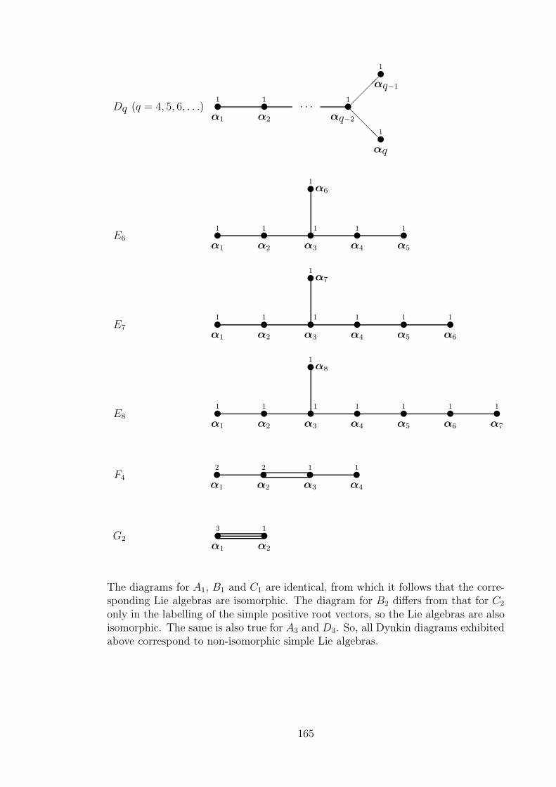
Dq (q = 4, 5, 6, . . .)
@@@@
• • •
•
•
· · ·α1 α2 αq−2
αq−1
αq
1 1 1
1
1
E6 • • • • •
•
α1 α2 α3 α4 α5
α6
1 1 1 1 1
1
E7 • • • • • •
•
α1 α2 α3 α4 α5 α6
α7
1 1 1 1 1 1
1
E8 • • • • • • •
•
α1 α2 α3 α4 α5 α6 α7
α8
1 1 1 1 1 1 1
1
F4 • • • •α1 α2 α3 α4
2 2 1 1
G2 • •α1 α2
3 1
The diagrams for A1, B1 and C1 are identical, from which it follows that the corre-sponding Lie algebras are isomorphic. The diagram for B2 differs from that for C2
only in the labelling of the simple positive root vectors, so the Lie algebras are alsoisomorphic. The same is also true for A3 and D3. So, all Dynkin diagrams exhibitedabove correspond to non-isomorphic simple Lie algebras.
165

11.6 The Dynkin diagram for SU(3).
In this section we study the Dynkin diagram A2, given by:
• •α β
1 1(11.37)
The diagram has two points and hence there are two simple positive root vectors,which are indicated by α and β. Moreover, because the number of simple positiveroot vectors equals the dimension of the Cartan subalgebra, the rank of the groupequals 2 (see section 11.2 for the definition of the rank of a Lie group). The twopoints are connected by one line, so the product nn′ defined in ( 11.34) equals 1,and therefore n = n′ = 1. This leads, by the use of formula ( 11.26), to:
α · βα ·α = −1
2and |α| = |β| = 1 . (11.38)
The latter relation can also be concluded from the absolute weight factors whichare indicated in the Dynkin diagram of formula ( 11.37). As a consequence of theequations ( 11.38), we find that the angle between the simple positive root vectorsα and β equals 120. In the figure below we show the two root vectors for this casein the corresponding two-dimensional root diagram.
-2nd
+1−1
6
1st
+√32
−√32
-α
AA
AA
AA
AAK
β
Figure 11.1: The simple positive root vectors α and β defined in formula ( 11.37)in the corresponding two-dimensional root diagram.
There is however a problem with the choice of the first and the second axis in theroot diagram. When we take the usual x-axis as the first and the y-axis as thesecond axis, then the first component of β becomes negative, −1
2, which contradicts
the definition of β as a simple positive root. This problem can be solved by selecting
166

the y-axis as the first axis and the x-axis as the second, as indicated in the rootdiagram of figure ( 11.1). In that case we find for α and β the following vectors:
α = (0, 1) and β = (+√32,−1
2) . (11.39)
The string ( 11.26) has here length n = 1, i.e.
β , β +α .
So, α+β is the third and also the only non-simple positive root vector. The corre-sponding negative root vectors are:
−α , −β and −α− β .
In figure ( 11.2) we show all root vectors in the root diagram for the group corre-sponding to the Dynkin diagram of formula ( 11.37).
- 2+1
2+1−1
2−1
6
1
+√32
−√32
-α
−α
α+ β
−α− β
AA
AA
AA
AAK
β
AAAAAAAAU −β
Figure 11.2: All root vectors which follow from the Dynkin diagram given in formula( 11.37).
When we compare the above root diagram for the step operators of the Lie groupgiven by formula ( 11.37) with figure ( 10.2) at page 134 for the step operatorsof SU(3), we come to the conclusion that both root diagrams are identical andtherefore both Lie algebras isomorphic, as we will see in the following.As mentioned before, the Cartan subalgebra has two basis elements, say H1 and
H2. Following formula ( 11.17) and using the results of formula ( 11.39), we obtainthe commutation relations for H1 and H2 with the step operators Eα and Eβ , i.e.
[H1 , Eα] = α1 Eα = 0 ,[
H1 , Eβ
]
= β1 Eβ = +√32Eβ ,
[H2 , Eα] = α2 Eα = Eα and[
H2 , Eβ
]
= β2 Eβ = −12Eβ .
(11.40)
167

When we compare those relations with the commutation relations for SU(3) givenin formula ( 10.7), then we find the following identifications:
H1 =M , H2 = I3 , Eα = I+ and Eβ = L+ .
When one also determines the other commutation relations, for example:
[
H1 , Eα + β
]
= (α1 + β1) Eα + β = +√32Eα + β and
[
H2 , Eα + β
]
= (α2 + β2) Eα + β = +12Eα + β ,
then one finds moreover:
Eα + β = K+ , E−α = I− , E−β = L− and E−α − β = K− .
The Lie algebra is now completely known and irreps can be constructed. Noticethat all this information is contained in the Dynkin diagram of formula ( 11.37).
168

Chapter 12
The orthogonal group in fourdimensions.
Rotations in four dimensions may not seem relevant for physics, but incidentelySO(4) is the symmetry group of (distance)−1 potentials, like the Newton gravita-tional potential and the Coulomb potential for the Hydrogen atom. We will studythis group in some detail, because it is also closely related to the symmetries ofspecial relativity.
12.1 The generators of SO(N).
The logarithm of any real, unimodular, orthogonal N × N matrix is, according tothe results of chapter 5 (see formulas 5.22 and 5.24), a real, traceless and anti-symmetric N × N matrix. Moreover, the diagonal elements of an anti-symmetricmatrix are zero. Consequently, an anti-symmetric matrix is automatically traceless.An elementary set of real, antisymmetric N × N matrices is formed by the set ofmatrices Mab (a, b = 1, 2, . . .N), whose matrix elements are defined by:
(
Mab
)
kℓ= −δakδbℓ + δaℓδbk , (12.1)
i.e. matrix element ab of Mab (a 6= b) equals −1, matrix element ba of Mab (a 6= b)equals +1 and all other of its matrix elements vanish.The matrices Mab are not all independent, because of the following properties:
Mba = −Mab and M11 = M22 = · · ·MNN = 0 . (12.2)
As a consequence, one ends up with a set of 12(N2 − N) independent matrices
Mab. This set forms a basis for the space of generators of the group SO(N). Anyreal, unimodular, orthogonal N ×N matrix O can be written as the exponent of alinear combination of the matrices Mab, as follows:
O(α) = exp
N∑
i, j = 1
12αijMij
. (12.3)
As a consequence of property ( 12.2), one may choose for the set of real constantsαij the properties:
169

αji = −αij and α11 = α22 = · · ·αNN = 0 . (12.4)
This implies that all real, unimodular, orthogonal N × N matrices can be para-metrized by a set of 1
2(N2−N) independent parameters. Consequently, SO(N) is a
12N(N − 1) parameter group. SO(2) is thus a one parameter group, SO(3) a three
parameter group and SO(4) a six parameter group.Alternatively, one might define the set of purely imaginary, traceless, Hermitean
N ×N matrices Mab, defined by:
Mab = iMab . (12.5)
Then, substituting definition ( 12.5) into expression ( 12.3) we find that any real,unimodular, orthogonal N ×N matrix O can be written as the exponent of a linearcombination of the matrices Mab, as follows:
O(α) = exp
N∑
i, j = 1− i
2αijMij
. (12.6)
For the generators Mab of SO(N) one has the following commutation relations:
[Mab , Mcd] = i
δacMbd + δbdMac − δadMbc − δbcMad
. (12.7)
In order to proof the above relations, we determine one of the matrix elements ofthe commutator in ( 12.7), using the definitions ( 12.1) and ( 12.5):
(
[Mab , Mcd])
ij=
(
MabMcd −McdMab
)
ij
=(
Mab
)
ik
(
Mcd
)
kj−(
Mcd
)
ik
(
Mab
)
kj
= −(
δaiδbk − δakδbi
) (
δckδdj − δcjδdk
)
+
+(
δciδdk − δckδdi
) (
δakδbj − δajδbk
)
= δac
δbiδdj − δdiδbj
+ δbd
δaiδcj − δciδaj
+
+ δad
δciδbj − δbiδcj
+ δbc
δdiδaj − δaiδdj
= δaci(
Mbd
)
ij+ δbdi (Mac)ij + δadi
(
Mcb
)
ij+ δbci
(
Mda
)
ij
= i
δacMbd + δbdMac − δadMbc − δbcMad
ij,
which shows the equality ( 12.7) for each matrix element and thus proofs relations( 12.7).
170

12.2 The generators of SO(4).
For the six parameter group SO(4) we define the following six generators:
L1 =M23 , L2 =M31 , L3 =M12 ,
K1 =M14 , K2 =M24 , K3 =M34 . (12.8)
Or, using the property ( 12.2) of the matrices Mab, in a more compact notation:
Li =12ǫijkMjk (i, j, k = 1, 2, 3) and Ki =Mi4 (i = 1, 2, 3) . (12.9)
The related matrices are explicitly given by:
L1 =
· · · ·· · −i ·· i · ·· · · ·
, L2 =
· · i ·· · · ·−i · · ·· · · ·
, L3 =
· −i · ·i · · ·· · · ·· · · ·
,
(12.10)
K1 =
· · · −i· · · ·· · · ·i · · ·
, K2 =
· · · ·· · · −i· · · ·· i · ·
, K3 =
· · · ·· · · ·· · · −i· · i ·
.
(12.11)Using the commutation relations ( 12.7) for the matrices Mab, we find for the
generators ~L and ~K the following commutation relations:
[Li , Lj ] = iǫijkLk , [Li , Kj ] = iǫijkKk and [Ki , Kj ] = iǫijkLk . (12.12)
The simple way to proof the above relations is just to use the explicit form of thecommutation relations ( 12.7) and the definitions ( 12.8), i.e.:
[L1 , L2] = [M23 , M31] = −iM21 = iM12 = iL3
[L2 , L3] = [M31 , M12] = −iM32 = iM23 = iL1
[L3 , L1] = [M12 , M23] = −iM13 = iM31 = iL2
[L1 , K1] = [M23 , M14] = 0
[L1 , K2] = [M23 , M24] = iM34 = iK3
[L1 , K3] = [M23 , M34] = −iM24 = −iK2
171

[L2 , K1] = [M31 , M14] = −iM34 = −iK3
[L2 , K2] = [M31 , M24] = 0
[L2 , K3] = [M31 , M34] = iM14 = iK1
[L3 , K1] = [M12 , M14] = iM24 = iK2
[L3 , K2] = [M12 , M24] = −iM14 = iK1
[L3 , K3] = [M12 , M34] = 0
[K1 , K2] = [M14 , M24] = iM12 = iL3
[K2 , K3] = [M24 , M34] = iM23 = iL1
[K3 , K1] = [M34 , M14] = iM31 = iL2
When we define the following six parameters:
n1 = α23 , n2 = α31 , n3 = α12 , k1 = α14 , k2 = α24 , k3 = α34 ,
then, using the relations ( 12.2), ( 12.4), ( 12.6) and ( 12.8), we may express anyreal, unimodular, orthogonal 4×4 matrix O by the exponent of a linear combinationof the matrices ~L and ~K, as follows:
O(
~n,~k)
= exp
−i~n · ~L− i~k · ~K
. (12.13)
From the commutation relations ( 12.12) for the generators ~L, one might observethat the transformations O(~n, 0) form a subgroup of SO(4) which is equivalent toSO(3). However, since the matricesO(~n, 0) are 4×4, they cannot form an irreduciblerepresentation of SO(3), since irreducible representations of SO(3) can only haveodd dimensions. The reduction of the 4 × 4 matrices O(~n, 0) is most convenientlystudied by determining the Casimir operator L2 for the four dimensional represen-tation, i.e. L2 = (L1)
2 + (L2)2 + (L3)
2. Using the explicit expressions ( 12.10) and( 12.11), we obtain for L2 the following result:
L2 =
2 · · ·· 2 · ·· · 2 ·· · · 0
.
We find that the four dimensional representation of the subgroup SO(3) of SO(4)can easily be reduced into two irreducible representations of SO(3): one of dimensionthree (L2 = 2), and one of dimension one (L2 = 0).
172

In order to construct irreducible representations of SO(4) it is convenient to in-troduce yet another set of generators for this group, i.e.:
~A = 12
(
~L+ ~K)
and ~B = 12
(
~L− ~K)
. (12.14)
When, using the expression ( 12.13), we define the following six parameters:
~a = ~n+ ~k and ~b = ~n− ~k ,
then we may express any real, unimodular, orthogonal 4× 4 matrix O by the expo-nent of a linear combination of the matrices ~A and ~B, as follows:
O(
~a,~b)
= exp
−i~a · ~A− i~b · ~B
. (12.15)
The commutation relations for the generators ~A and ~B can easily be obtained,using the relations ( 12.12)
[Ai , Aj ] = iǫijkAk , [Bi , Bj ] = iǫijkBk and [Ai , Bj ] = 0 . (12.16)
Because of the latter commutation relation and relation ( 12.15), remembering theBaker-Campbell-Hausdorf relations, we may express any real, unimodular, orthog-onal 4 × 4 matrix O by the product of two exponents: one of a linear combinationof the matrices ~A and one of a linear combination of the matrices ~B, as follows:
O(
~a,~b)
= exp
−i~a · ~A
exp
−i~b · ~B
. (12.17)
The matrices ~A and ~B are explicitly given by:
A1 =1
2
· · · −i· · −i ·· i · ·i · · ·
, A2 =
1
2
· · i ·· · · −i−i · · ·· i · ·
, A3 =
1
2
· −i · ·i · · ·· · · −i· · i ·
,
(12.18)
B1 =1
2
· · · i· · −i ·· i · ·−i · · ·
, B2 =
1
2
· · i ·· · · i−i · · ·· −i · ·
, B3 =
1
2
· −i · ·i · · ·· · · i· · −i ·
.
(12.19)
The generator subset formed by the matrices ~A generates a subgroup SA of SO(4)which, because of the commutation relations ( 12.16), is equivalent either to SO(3)
or to SU(2), and similar for the generator subset formed by the matrices ~B. Fromexpressions ( 12.18) and ( 12.19) it is easy to determine the Casimir operators A2
and B2 for each of the two subspaces of SO(4). One finds A2 = 34and B2 = 3
4.
Consequently, the subgroup SA of real, unimodular, orthogonal 4×4 matricesO(~a, 0)may be reduced to a two-dimensional representation of the group SU(2) as well as
173

the subgroup SB of real, unimodular, orthogonal 4 × 4 matrices O(0,~b). This canbe shown more explicitly, using the following similarity transformation S:
S =1√2
1 0 0 −1i 0 0 i0 −1 −1 00 −i i 0
with S−1 =1√2
1 −i 0 00 0 −1 i0 0 −1 −i−1 −i 0 0
.
When we apply this basis transformation to the matrices ( 12.18) and ( 12.19),we find:
S−1 ~AS =~σ
2⊗ 1 and S−1 ~BS = 1⊗ ~σ
2. (12.20)
Consequently, for any real, unimodular, orthogonal 4× 4 matrix O we obtain:
S−1O(
~a,~b)
S = exp
−i~a · ~σ2
⊗ exp
−i~b · ~σ2
. (12.21)
Each group element O(
~a,~b)
of SO(4) is equivalent to the direct product of
two group elements U (~a ) = exp
−i~a · ~σ2
and U(
~b)
= exp
−i~b · ~σ2
of SU(2).
Consequently, SO(4) is homomorphous with SU(2) ⊗ SU(2). However, those twogroups are not equal.
12.3 The group SU(2) ⊗ SU(2).
We represent the direct product U(
~a,~b)
of two elements U (~a) and U(
~b)
of SU(2)in the following abstract way, by:
U(
~a,~b)
=(
U (~a) , U(
~b))
. (12.22)
The group product is defined in analogy with the product ( 5.29) of two directproducts of two matrices, as follows:
U(
~a,~b)
U(
~c, ~d)
=(
U (~a)U (~c) , U(
~b)
U(
~d))
. (12.23)
It is easy to verify that under the product ( 12.23) the elements ( 12.22) form agroup, the group SU(2)⊗ SU(2): For example, the identity element I is given by:
I = U(0, 0) = (1 , 1) , (12.24)
and the inverse of group element U(
~a,~b)
by (compare formula ( 5.30)):
[
U(
~a,~b)]−1
=(
[U (~a)]−1 ,[
U(
~b)]−1
)
. (12.25)
The structure of SU(2)⊗ SU(2) is similar to the structure of SO(4) as described
in section ( 12.2). Their algebras are equal. The generators ~A and ~B defined informula ( 12.14) and in detail related to SU(2)⊗ SU(2) in formula ( 12.20), might
here, using the operators ~J for SU(2) defined in formula ( 9.15), be defined by:
174

~A =(σ
2, 0)
= ( ~J, 0) and ~B =(
0,σ
2
)
= (0, ~J) . (12.26)
The generators ~A generate the subgroup SA = (U (~a) ,1) of SU(2) ⊗ SU(2),
and the generators ~B the subgroup SB =(
1, U(
~b))
. The group elements of
SU(2) ⊗ SU(2) can be represented by direct products of matrices. An irreduciblerepresentation is fully determined by the eigenvalues of the two Casimir operatorsA2 and B2, or alternatively by ja and jb, i.e.
D(ja, jb)(
U(
~a,~b))
= D(ja) (U (~a))⊗D(jb)(
U(
~b))
=
e−i~a · d(ja)( ~J)
⊗
e−i~b · d(jb)( ~J)
. (12.27)
The dimension of the irreducible representation is given by:
dim(
D(ja, jb))
= (2ja + 1)(2jb + 1) . (12.28)
The first few irreps of SU(2)⊗SU(2) and their dimensions are listed in the table( 12.1).
d (ja, jb) d (ja, jb)
1 (0,0) 9 (1,1), (0,4), (4,0)
2 (0,12), (1
2,0) 10 (0,9
2), (9
2,0), (2,1
2), (1
2,2)
3 (0,1), (1,0) 11 (0,5), (5,0)
4 (0,32), (3
2,0), (1
2,12) 12 (0,11
2), (11
2,0), (1
2,52), (5
2,12), (1,3
2), (3
2,1)
5 (0,2), (2,0) 13 (0,6), (6,0)
6 (0,52), (5
2,0), (1,1
2), (1
2,1) 14 (0,13
2), (13
2,0), (3,1
2), (1
2,3)
7 (0,3), (3,0) 15 (0,7), (7,0), (1,2), (2,1)
8 (0,72), (7
2,0), (1
2,32), (3
2,12) 16 (0,15
2), (15
2,0) (1
2,72), (7
2,12), (3
2,32)
Table 12.1: Irreps of SU(2)⊗ SU(2) and their dimensions (d).
175

As an example, let us study the two dimensional irrep (0,12) of SU(2)⊗SU(2). A
group element U(
~a,~b)
is, according to formula ( 12.27), represented by:
D(0, 12)(
U(
~a,~b))
= D(0) (U (~a))⊗D(12)(
U(
~b))
=
e0
⊗
e−i~b · ~σ2
= 1⊗
e−i~b · ~σ2
= e
−i~b · ~σ2 , (12.29)
which represents a 2× 2 matrix.The two dimensional irrep (0,1
2) is not a faithfull representation of SU(2)⊗SU(2),
as one has:
D(0, 12)(
U(
~a1,~b))
= D(0, 12)(
U(
~a2,~b))
for all ~a1 and ~a2 .
The identity I=(1,1) is, as always, represented by the unit matrix, according to:
D(0, 12) (I) = D(0) (1)⊗D(
12) (1) = 1⊗ 1 =
(
1 00 1
)
.
The group element (−1,−1) is represented by the minus unit matrix, accordingto:
D(0, 12) ((−1,−1)) = D(0) (−1)⊗D(
12) (−1) = 1⊗ (−1) = −
(
1 00 1
)
.
Notice from the above two expressions that for the two dimensional irrep (0,12)
one has:
D(0, 12) ((1,1)) 6= D(0, 1
2) ((−1,−1)) .
This is not always the case. For example, for the four dimensional irrep (12,12) one
finds:
D(12, 12) ((1,1)) = 1⊗1 =
1 · · ·· 1 · ·· · 1 ·· · · 1
= (−1)⊗(−1) = D(12, 12) ((−1,−1)) .
(12.30)and similar:
D(12, 12)((
U (~a) , U(
~b)))
= U (~a)⊗ U(
~b)
= −U (~a) ⊗
−U(
~b)
= D(12, 12)((
−U (~a) ,−U(
~b)))
. (12.31)
176

So, also the four dimensional irrep (12,12) is not faithfull, since sets of two elements
of SU(2)⊗ SU(2) are represented by the the same matrix.
12.4 The relation between SO(4) and SU(2) ⊗
SU(2).
As we have seen in formula ( 12.21), each group element O(
~a,~b)
of SO(4) is
equivalent to the direct product of two group elements U (~a ) = exp
−i~a · ~σ2
and
U(
~b)
= exp
−i~b · ~σ2
of SU(2). Consequently, SO(4) is isomorphous to the four
dimensional irrep (12,12) of SU(2)⊗ SU(2). Which implies that each group element
of SO(4) is equivalent to two different group elements of SU(2)⊗ SU(2).The set of group elements of SU(2)⊗SU(2) indicated by (1,1) , (−1,−1) is
called the kernel of the homomorphism of SU(2) ⊗ SU(2) onto SO(4). When wedivide SU(2) ⊗ SU(2) by this kernel, which means that when we either consider
group element(
U (~a) , U(
~b))
or group element(
−U (~a) ,−U(
~b))
, then we obtain
the following isomorphism for SO(4):
SO(4) =SU(2)⊗ SU(2)
(1,1) , (−1,−1) . (12.32)
12.5 Irreps for SO(4).
Let us compare the above relation ( 12.32) with the relation between SO(3) andSU(2). All irreps for SO(3) can be obtained from the irreps of SU(2), providedthat we eliminate those irreps of SU(2) for which D(1) 6= D(−1), i.e. those witheven dimensions. For SO(4) the situation is similar: From all irreps of SU(2)⊗SU(2)we just must eliminate those for which:
D ((1,1)) 6= D ((−1,−1)) . (12.33)
When we denote the eigenvalues of A2 by 2ja + 1 and of B2 by 2jb + 1, then, aswe have seen in formula ( 12.27), a general irrep for SU(2)⊗SU(2) may be writtenin the form
D(ja, jb)((
U (~a) , U(
~b)))
= D(ja) (U (~a ))⊗D(jb)(
U(
~b))
. (12.34)
Now, for the element −1 of SU(2), one has:
D(j) (−1) =
D(j) (1) , j = 0, 1, 2, 3, . . .
−D(j) (1) , j = 12, 32, 52, . . .
. (12.35)
Consequently, using relation ( 12.34), one obtains for the representation of thecomparable group elements of SU(2)⊗ SU(2) the following:
177

D(ja, jb) ((−1,−1)) =
D(ja, jb) ((1,1)) , ja + jb = 0, 1, 2, 3, . . .
−D(ja, jb) ((1,1)) , ja + jb =12, 32, 52, . . .
.
(12.36)Now, since for SO(4) we must eliminate those irreps of SU(2)⊗ SU(2) for which
relation ( 12.33) holds, we find as a result from the above formula ( 12.36) that:
ja + jb = integer ⇔
either ja and jb both integer
or ja and jb both half-integer. (12.37)
The dimension of an irrep of SO(4) is given by:
dim(
D(ja, jb))
= (2ja + 1)(2jb + 1) . (12.38)
In table ( 12.2), we indicate the first few irreps of SO(4) and their dimension:
dimension (ja, jb) dimension (ja, jb)
1 (0,0) 9 (1,1), (0,4), (4,0)
2 - 10 -
3 (0,1), (1,0) 11 (0,5), (5,0)
4 (12,12) 12 (1
2,52), (5
2,12)
5 (0,2), (2,0) 13 (0,6), (6,0)
6 - 14 -
7 (0,3), (3,0) 15 (0,7), (7,0), (1,2), (2,1)
8 (12,32), (3
2,12) 16 (1
2,72), (7
2,12), (3
2,32)
Table 12.2: Irreps of SO(4) and their dimension.
From this table, we notice that for some dimensions (2, 6 ,10, 14, . . .) SO(4) hasno corresponding irreps. Whereas for other dimensions more than one inequivalentirrep exist. There are, for instance, two three dimensional irreps, namely (ja = 0,jb = 1) and (ja = 1, jb = 0). Let us, as an example, show that those two irreps arenot equivalent:For the first irrep (ja = 0, jb = 1) we have the representations:
d(0,1)( ~A) = 0 and d(0,1)( ~B) = ~L , (12.39)
where ~L represents the three 3× 3 matrices given in formula ( 8.24). For the group
element O(
~a,~b)
of SO(4) we obtain then the representation:
178

D(0,1)(
O(
~a,~b))
= exp
−i~a · d(0,1)( ~A)
⊗ exp
−i~b · d(0,1)( ~B)
= 1⊗ e−i~b · ~L = e−i~b · ~L , (12.40)
which represents a 3× 3 matrix.Similarly, for the other irrep (ja = 1, jb = 0) we have the representations:
d(1,0)( ~A) = ~L and d(1,0)( ~B) = 0 , (12.41)
leading for the representation of the group element O(
~a,~b)
of SO(4) to the expres-sion:
D(1,0)(
O(
~a,~b))
= e−i~a · ~L . (12.42)
Now, representations (ja = 0, jb = 1) and (ja = 1, jb = 0) are equivalent when
there exists a similarity transformation S, such that for all possible ~a and ~b yields:
S−1 D(0,1)(
O(
~a,~b))
S = D(1,0)(
O(
~a,~b))
, (12.43)
which, using the expressions ( 12.40) and ( 12.42), amounts in finding a basis trans-formation S such that:
S−1 e−i~b · ~L S = e−i~a · ~L , (12.44)
or at the level of the algebra, such that:
S−1 ~b · ~L S = ~a · ~L for all ~a and ~b . (12.45)
This relation must hold for arbitrary and independent ~a and~b, which is impossiblefor one single transformation S. Consequently, the two irreps (ja = 0, jb = 1) and(ja = 1, jb = 0) are not equivalent.
12.6 Weight diagrams for SO(4).
Let us for the irreducible representation D(ja, jb), select basis vectors |ma, mb >which are simultaneously eigenvectors for d(ja, jb) (A3) and d
(ja, jb) (B3) with eigen-values ma and mb respectively, i.e.:
d(ja, jb) (A3) |ma, mb > = ma |ma, mb > and
d(ja, jb) (B3) |ma, mb > = mb |ma, mb > . (12.46)
One might, in analogy with SO(3), also define the step operators A± = A1 ± iA2
for which:
179
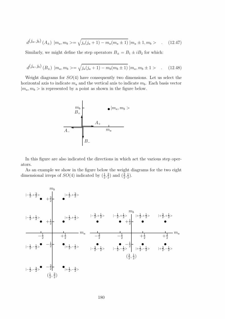
d(ja, jb) (A±) |ma, mb >=√
ja(ja + 1)−ma(ma ± 1) |ma ± 1, mb > . (12.47)
Similarly, we might define the step operators B± = B1 ± iB2 for which:
d(ja, jb) (B±) |ma, mb >=√
ja(ja + 1)−mb(mb ± 1) |ma, mb ± 1 > . (12.48)
Weight diagrams for SO(4) have consequently two dimensions. Let us select thehorizontal axis to indicate ma and the vertical axis to indicate mb. Each basis vector|ma, mb > is represented by a point as shown in the figure below.
ma
mb • |ma, mb >
- A+
A−
6B+
?B−
In this figure are also indicated the directions in which act the various step oper-ators.As an example we show in the figure below the weight diagrams for the two eight
dimensional irreps of SO(4) indicated by (12,32) and (3
2,12).
(12, 32)
•
•
•
•
•
•
•
•
mb
ma−12
+12
+32
+12
−12
−32|−1
2 ,−32>
|−12 ,−
12>
|−12 ,+
12>
|−12 ,+
32>
|+12 ,−
32>
|+12 ,−
12>
|+12 ,+
12>
|+12 ,+
32>
(32, 12)
• • • •
• • • •
mb
ma−32
−12
+12
+32
+12
−12
|−32 ,−
12> |−1
2 ,−12> |+1
2 ,−12> |+3
2 ,−12>
|−32 ,+
12> |−1
2 ,+12> |+1
2 ,+12> |+3
2 ,+12>
180
12.7 Invariant subgroups of SO(4).
In this section we show that the sets of group elements SA = O(~a, 0) and SB =
O(0,~b)
are invariant subgroups of SO(4). Let us, using the expression ( 12.21),
represent group element O(~a,~b) of SO(4) by:
O(
~a,~b)
= S
U (~a )⊗ U(
~b)
S−1 . (12.49)
According to the definition of an invariant subgroup of a group, which is given informula ( 1.24), we must concentrate on the following expression:
[
O(
~α, ~β)]−1O
(
~a,~b) [
O(
~α, ~β)]
. (12.50)
Inserting the above expression ( 12.49) and using formula ( 5.30), we obtain:
S
[U (~α )]−1 ⊗[
U(
~β)]−1
S−1S
U (~a )⊗ U(
~b)
S−1S
U (~α )⊗ U(
~β)
S−1 .
Next, using the property ( 5.29) for the product of direct products of matrices,we obtain:
S(
[U (~α )]−1 U (~a )U (~α )
⊗[
U(
~β)]−1
U(
~b)
U(
~β))
S−1 .
In case that the group element O(~a,~b) belongs to one of the two subgroups SA orSB, we find in particular:
S(
[U (~α )]−1 U (~a )U (~α )
⊗ 1)
S−1 for ~b = 0,
S(
1⊗[
U(
~β)]−1
U(
~b)
U(
~β))
S−1 for ~a = 0.
This can be written in terms of the transformed vectors ~a ′ and ~b ′, according to:
S (U (~a ′)⊗ 1)S−1 for ~b = 0,
S(
1⊗ U(
~b ′))
S−1 for ~a = 0.
(12.51)
So, we find that under the transformation ( 12.50) each subgroup element O(~a, 0)of SA is transformed into another (or the same) subgroup element of SA and similarfor SB. It implies that for an arbitrary element O of SO(4) we have:
O−1 SA O = SA and O−1 SB O = SB . (12.52)
Consequently, SA and SB are invariant subgroups of SO(4). From the commu-
tation relations ( 12.16) for the generators ~A of SA and ~B of SB, we conclude thatthose subgroups are moreover not Abelian.One may show in general that SO(4) has non-trivial invariant subgroups, but no
non-trivial Abelian invariant subgroups. Such a group is called semi-simple.
181

12.8 The Hydrogen atom
As an application of the representations of SO(4) we study in this section the Hy-drogen atom.
1. Classically
Classically, the equations of motion of a charged spinless particle in a centralatractive Coulomb field (or a massive particle in a gravitational field) can be derivedfrom the following Lagrangian:
L(
~r, ~r)
= 12~r 2 +
1
r. (12.53)
The equations of motion are given by:
~r = − ~r
r3. (12.54)
Associated with the Lagrangian ( 12.53) are the following two conserved quanti-ties:
The orbital angular momentum ~L = ~r × ~r d~Ldt = 0
The Runge-Lenz vector ~M = −~r × ~L+ ~rr
d ~Mdt = 0
Using the equations of motion ( 12.54), it is easy to show that the above quantitiesare conserved:
d~L
dt= ~r × ~r + ~r × ~r = 0 + ~r ×
(
− ~r
r3
)
= 0.
d ~M
dt= −~r × ~L− ~r × ~L+
~r
r− ~r
r3
(
~r · ~r)
=~r
r3× ~L− 0 +
~r
r− ~r
r3
(
~r · ~r)
=~r
r3×(
~r × ~r)
+~r
r− ~r
r3
(
~r · ~r)
=1
r3
~r(
~r · ~r)
− ~r (~r · ~r)
+~r
r− ~r
r3
(
~r · ~r)
= 0
The Runge-Lenz vector for a bound state solution of the equations of motion(elipse) points from the force center towards the perihelion of the elipse. The mod-
ulus of ~M equals the excentricity of the orbit.
182
2. Quantum Mechanically
In Quantum Mechanics, the equations of motion are given by the following Hamil-tonian:
H = ~r · ~p− L(
~r, ~r)
= 12~p 2 − 1
rwith ~p =
∂L∂~r
= ~r . (12.55)
In comparison with the classical case, one may derive from this Hamiltonian thefollowing constants of motion:
~L = ~r × ~p and ~M = 12
~L× ~p− ~p× ~L
+~r
r. (12.56)
It may be verified that both ~L and ~M commute with the Hamiltonian, i.e.
[H , ~L] = [H , ~M ] = 0 . (12.57)
Furthermore, one has the expression:
~L · ~M = ~M · ~L = 0; . (12.58)
When we define next the following operators:
~A = 12
(
~L+ ~M)
and ~B = 12
(
~L− ~M)
, (12.59)
then we may verify for ~A and ~B the same commutation relations as those given informula ( 12.16). Moreover, using the commutation relations ( 12.57), it may be
clear that ~A and ~B commute with the Hamiltonian ( 12.55), and using the identity( 12.58), it follows that the Casimir operators A2 and B2 satisfy the relation:
A2 − B2 = ~L · ~M = 0 . (12.60)
The group associated with the operators ~A and ~B is evidently SO(4). Conse-quently, we may expect that the eigenstates of the Hamiltonian ( 12.55) can begrouped into irreps of SO(4).Eigenstates of the Schrodinger equation may then be chosen such that they are
simultaneously eigenstates of d(A3) and d(B3), i.e.:
H |n,ma, mb > ∼ − 1
n2 |n,ma, mb > ,
d(A3) |n,ma, mb > = ma |n,ma, mb > and
d(B3) |n,ma, mb > = mb |n,ma, mb > . (12.61)
For the Casimir operators A2 and B2 one finds:
A2 |n,ma, mb > = ja(ja + 1) |n,ma, mb > and
B2 |n,ma, mb > = jb(jb + 1) |n,ma, mb > . (12.62)
183

However, because of the relation ( 12.60), one has an extra condition for thepossible irreps of SO(4) into which the eigenstates of the Hamiltonian ( 12.55) canbe grouped, i.e.
ja(ja + 1)− jb(jb + 1) = 0 ⇔ ja = jb . (12.63)
Eigenstates which belong to the same irrep (ja, ja) of SO(4) must have the sameenergy eigenvalues, because of the commutation relations ( 12.57). Consequently,the degeneracy of an energy level is given by the dimension of the associated irrep.For the permitted irreps of SO(4) we obtain dimensions 1, 4, 9, 16, . . . , which caneasily be verified to be in agreement with the degeneracies of the solutions of theSchrodinger equation for Hydrogen. In order to see that, we might select a basis forthe eigenstates of the Schrodinger equation which are simultaneously eigenstates ofL2 and d(L3), i.e.:
H |n, ℓ, ℓz > ∼ − 1
n2 |n, ℓ, ℓz > , n = 1, 2, 3, . . .
L2 |n, ℓ, ℓz > = ℓ(ℓ+ 1) |n, ℓ, ℓz > , ℓ < n , and
d(L3) |n, ℓ, ℓz > = ℓz |n, ℓ, ℓz > , |ℓz| ≤ ℓ . (12.64)
Below we compare the degeneracies for the two different bases, ( 12.61) and( 12.64), for the first few levels of Hydrogen:
ja (2ja + 1)2 energy level, n ℓ < n number of states
0 1 1 0 1
12
4 2 0,1 1+3=4
1 9 3 0,1,2 1+3+5=9
32
16 4 0,1,2,3 1+3+5+7=16
2 25 5 0,1,2,3,4 1+3+5+7+9=25
184

185