efficient multiway thetajoin processing using...
TRANSCRIPT
Efficient Multi-way Theta-Join Processing UsingMapReduce
Xiaofei ZhangHKUST
Hong Kong
Lei ChenHKUST
Hong Kong
Min WangHP Labs ChinaBeijing, China
ABSTRACT
Multi-way Theta-join queries are powerful in describing com-plex relations and therefore widely employed in real prac-tices. However, existing solutions from traditional distribut-ed and parallel databases for multi-way Theta-join queriescannot be easily extended to fit a shared-nothing distributedcomputing paradigm, which is proven to be able to sup-port OLAP applications over immense data volumes. Inthis work, we study the problem of efficient processing ofmulti-way Theta-join queries using MapReduce from a cost-effective perspective. Although there have been some worksusing the (key,value) pair-based programming model to sup-port join operations, efficient processing of multi-way Theta-join queries has never been fully explored. The substantialchallenge lies in, given a number of processing units (thatcan run Map or Reduce tasks), mapping a multi-way Theta-join query to a number of MapReduce jobs and having themexecuted in a well scheduled sequence, such that the totalprocessing time span is minimized. Our solution mainly in-cludes two parts: 1) cost metrics for both single MapReducejob and a number of MapReduce jobs executed in a certainorder; 2) the efficient execution of a chain-typed Theta-joinwith only one MapReduce job. Comparing with the queryevaluation strategy proposed in [23] and the widely adoptedPig Latin and Hive SQL solutions, our method achieves sig-nificant improvement of the join processing efficiency.
1. INTRODUCTIONData analytical queries in real practices commonly in-
volve multi-way join operations. The operators involved in amulti-way join query are more than just Equi-join. Instead,the join condition can be defined as a binary function θ thatbelongs to {<,≤,=,≥,>,<>}, as known as Theta-join. Com-pared with Equi-join, it is more general and expressive inrelation description and surprisingly handy in data analyticqueries. Thus, efficient processing of multi-way Theta-joinqueries plays a critical role in the system performance. Infact, evaluating multi-way Theta-joins has always been a
challenging problem along with the development of databasetechnology. Early works, like [8][26][22] and etc., have elab-orated the complexity of the problem and presented theirevaluation strategies. However, their solutions do not scaleto process the multi-way Theta-joins over the data of tremen-dous volumes. For instance, as reported from Facebook [5]and Google [11], the underlying data volume is of hundredsof tera-bytes or even peta-bytes. In such scenarios, solu-tions from the traditional distributed or parallel databasesare infeasible due to unsatisfactory scalability and poor faulttolerance.
On the contrary, (key,value)-based MapReduce program-ming model substantially guarantees great scalability andstrong fault tolerance property. It has emerged as the mostpopular processing paradigm in a shared-nothing computingenvironment. Recently, devoting research efforts towards ef-ficient and effective analytic processing over immense datahave been made within the MapReduce framework. Cur-rently, the database community mainly focuses on two is-sues. First, the transformation from certain relational al-gebra operator, like similarity join, to its (key,value)-basedparallel implementation. Second, the tuning or re-designof the transformation function such that the MapReducejob is executed more efficiently in terms of less time cost orcomputing resources consumption. Although various rela-tional operators, like pair-wise Theta-join, fuzzy join, aggre-gation operators and etc., are evaluated and implementedusing MapReduce, there is little effort exploring the effi-cient processing of multi-way join queries, especially moregeneral computation namely Theta-join, using MapReduce.The reason is that, the problem involves more than just arelational operator→(key,value) pair transformation and thetuning, there are other critical issues needed to be addressed:1) How many MapReduce jobs should we employ to evaluatethe query? 2) What is each MapReduce job responsible for?3) How should multiple MapReduce jobs be scheduled?
To address the problem, there are two challenging issuesneeded to be resolved. Firstly, the number of available com-puting units is in fact limited, which is often neglected whenmapping a task to a set of MapReduce jobs. Althoughthe pay-as-you-go policy of Cloud computing platform couldpromise as many computing resources as required, however,once a computing environment is established, the allowedmaximum number of concurrent Map and Reduce tasks isfixed according to the system configuration. Even takenthe auto scaling feature of Amazon EC2 platform [18] intoconsideration, the maximum number of involved computingunits are pre-determined by the user-defined profiles. There-
1184
Permission to make digital or hard copies of all or part of this work forpersonal or classroom use is granted without fee provided that copies arenot made or distributed for profit or commercial advantage and that copiesbear this notice and the full citation on the first page. To copy otherwise, torepublish, to post on servers or to redistribute to lists, requires prior specificpermission and/or a fee. Articles from this volume were invited to presenttheir results at The 38th International Conference on Very Large Data Bases,August 27th - 31st 2012, Istanbul, Turkey.Proceedings of the VLDB Endowment, Vol. 5, No. 11Copyright 2012 VLDB Endowment 2150-8097/12/07... $ 10.00.
fore, with the user specified Reduce task number, a multi-way Theta-join query is processed with only limited numberof available computing units.
The second challenge is that, the decomposition of a multi-way Theta-join query into a number of MapReduce tasks isnon-trivial. Work [28] targets at the multi-way Equi-joinprocessing. It decomposes a query into several MapReducejobs and schedules the execution based on a specific costmodel. However, it only considers the pair-wise join as thebasic scheduling unit. In other words, it follows the tradi-tional multi-way join processing methodology, which eval-uates the query with a sequence of pair-wise joins. Thismethodology excludes the possible optimization opportunityto evaluate a multi-way join in one MapReduce job. Ourobservation is that, under certain conditions, evaluating amulti-way join with one MapReduce job is much more effi-cient than with a sequence of MapReduce jobs conductingpair-wise joins. Work [23] reports the same observation. Onedominating reason is that, the I/O costs of intermediate re-sults generated by multiple MapReduce jobs may becomeunacceptable overheads. Work [2] presents the solution ofevaluating a multi-way join in one MapReduce job, whichonly works for the Equi-join case. Since the Theta-join can-not be answered by simply making the join attribute thepartition key, thus, the solution proposed in [2] cannot be ex-tended to solve the case of multi-way Theta-joins. Work [25]demonstrates effective pair-wise Theta-join processing usingMapReduce by partitioning a two dimensional result spaceformed by the cross-product of two relations. For the caseof multi-way join, the result space is a hyper-cube, whosedimensionality is the number of the relations involved inthe query. Unfortunately, work [25] does not explore howto extend their solution to handle the partition in high di-mensions. Moreover, the question about whether we shouldevaluate a complex query with a single MapReduce job orseveral MapReduce jobs, is not clear yet. Therefore, thereis no straightforward solution to combine the techniques inexisting literatures to evaluate a multi-way Theta-join query.
Meanwhile, assume a set of MapReduce jobs are gener-ated for the query evaluation. Then given a limited numberof processing units, it remains a challenge to schedule theexecution of MapReduce jobs, such that the query can beanswered with the minimum time span. These jobs may havedependency relationships and inter-competition for resourceconsumptions during the concurrent execution. Currently,the MapReduce framework requires the number of Reducetasks as a user specified input. Thus, after decomposing amulti-way Theta-join query into a number of MapReducejobs, one challenging issue is how to specify each job aproper Reduce task number, such that the overall schedulingachieves the minimum execution time span.
Specifically, the problem that we are working on is: givena number of processing units (that can run Map or Re-duce tasks), mapping a multi-way Theta-join to a number ofMapReduce jobs and having them executed in a well sched-uled order, such that the total processing time span is mini-mized. Our solution to this challenging problem includes twocore techniques. The first one is, given a multi-way Theta-join query, we examine all the possible decomposition plansand estimate the minimum execution time cost for each plan.Especially, we figure out the rules to properly decompose theoriginal multi-way Theta-join query and study the most ef-ficient solution to evaluate multiple join condition functions
using one MapReduce job. The second technique is that,given a limited number of computing units and a pool ofpossible MapReduce jobs to evaluate the query, we design anovel solution to select jobs to effectively evaluate the queryas fast as possible. To evaluate the cost, we develop an I/Oand network aware cost model to describe the behavior of aMapReduce job.
To the best of our knowledge, this is the first work explor-ing the multi-way Theta-joins evaluation using MapReduce.Our main contributions are listed as follows:
• We establish the rules to decompose a multi-way joinquery. Under our proposed cost model, we can figureout whether a multi-way join query should be evalu-ated with multiple MapReduce jobs or a single MapRe-duce job.
• We develop a resource aware (key,value) pair distri-bution method to evaluate the chain-typed multi-wayTheta-join query with one MapReduce job, which guar-antees minimized volume of data copying over the net-work, as well as evenly distributed workload amongReduce tasks.
• We validate our cost model and the solution for multi-way Theta-join queries with extensive experiments.
The rest of the paper is organized as follows. In Section 2,we briefly review the MapReduce computing paradigm andelaborate the application scenario for multi-way Theta-joins.We formally define our problem in Section 3 and presentour cost model in section 4. We take Section 5 to explainour query evaluation strategies in details. We validate oursolution in Section 6 with extensive experiments on both realand synthetic data sets. We summarize and compare themost recent closely related work in Section 7 and concludeour work in Section 8.
2. PRELIMINARIESIn this section we briefly present the MapReduce program-
ming model and how it has been applied to evaluate joinqueries. More importantly, we elaborate the difficulties andlimitations of current solutions to solve the multi-way Theta-joins with a concrete example.
2.1 MapReduce & Join ProcessingMapReduce provides a simple parallel programming model
for data-intensive applications in a shared-nothing environ-ment [12]. It was originally developed for indexing crawledwebsites and OLAP applications. Generally, a Master nodeinvokes Map tasks on computing nodes that possess theinput data, which guarantees the locality of computation.Map tasks transform the input (key,value) pair (k1,v1) to n
new pairs: (k21,v
21), (k
22,v
22), ..., (k
2n,v
2n). The output of Map
tasks are then partitioned by the default hashing to differ-ent Reduce tasks according to k2
i . Once the Reduce tasksreceive (key,value) pairs grouped by k2
i , they perform theuser specified computation on all the values of each key, andwrite results back to the storage.
Obviously, this (key,value)-based programming model im-plies a natural implementation of Equi-join. By making thejoin attribute the key, records that can be joined togetherare sent to the same Reduce task. Even for the similarityjoin case [27], as long as the similarity metric is defined,each data record is assigned with a key set K = {ki, ..., kj},and the intersection of similar data records’ key sets is never
1185
empty. Thus, through such a mapping, it guarantees thatsimilar data records will be sent to at least one commonReduce task.
In fact, this key set method can be applied to any type ofjoin operator. However, to ensure that joinable data recordsare always assigned to overlapping key sets, the cardinalityof a data record’s K can be very large. In the worst case,it is the total number of Reduce tasks. Since the cardinal-ity of a record’s K implies the number of times this recordbeing duplicated among Reduce tasks, the larger the valueis, the more computing overheads in terms of I/O and CPUconsumption will be introduced. Therefore, the essential op-timization goal is to find “the optimal” assignment of K toeach data record, such that the join query can be evaluatedwith minimized data transmission over the network.
Another common concern about the MapReduce program-ming model is its poor immunity to key skews. If (key,value)pairs are highly unevenly distributed among Reduce tasks,the system throughput can degrade significantly. Unfortu-nately, this could be a common scenario in join operations.If there exist “popular” join attribute values, or the join con-dition is an inequality, some data records can be joined withhuge number of data records from other relations, whichimplies significant key skew among the Reduce tasks. More-over, the fault tolerance property of the MapReduce pro-gramming model is guaranteed on the cost of saving all theintermediate results. Thus, the overhead of disk I/O domi-nates the time efficiency of iterative MapReduce jobs. Thesame observation has been made in [28].
In summary, to efficiently process join operations usingMapReduce is non-trivial. Especially when it comes to multi-way join processing, selecting proper MapReduce jobs anddeciding a proper K for each data record make the problemmore challenging.
2.2 Multi-way Theta-JoinTheta-join is the join operation that takes inequality con-
ditions of join attributes’ values into consideration, namelythe join condition function θ ∈ {<,>,=, <>,≤,≥}. Multi-way Theta-join is a powerful analytic tool to elaborate com-plex data correlations. Consider the following applicationscenario:
“Assume we have n cities, {c1, c2, ..., cn}, and all theflights information FIi,j between any two cities ci and cj .Given a sequence of cities < cs, ..., ct >, and the stay-overtime length which must fall in the interval Li = [l1, l2] ateach city ci, find out all the possible travel plans.”This is a practical query that could help travelers plan
their trips. For illustration purpose, we simply assume FIi,jis a table containing flight No., departure time (dt) and ar-rival time (at). Then the above request can be easily an-swered with a multi-way Theta-join operation over FIs,s+1,..., FIt−1,t, by specifying the time interval between two suc-cessive flights falling into the particular city’s stay-over in-terval requirement. For example, the θ function betweenFIs,s+1 and FIs+1,s+2 is FIs,s+1.at+Ls+1.l1 < FIs+1,s+2.dt
< FIs,s+1.at+ Ls+1.l2.To evaluate such queries, a straightforward method is to
iteratively conduct pair-wise Theta-join. However, this eval-uation strategy might exclude some more efficient evaluationplans. For instance, instead of using pair-wise joins, we canevaluate multiple join conditions in one task. Therefore, lessMapReduce jobs are needed, which implies less computation
overheads in terms of the disk I/O of intermediate results.
3. PROBLEM DEFINITIONIn this work, we mainly focus on the efficient processing of
multi-way Theta-joins using MapReduce. Our solution tar-gets on the MapReduce job identification and scheduling.In other words, we work on the rules to properly decom-pose the query processing into several MapReduce jobs andhave them executed in a well scheduled fashion, such thatthe minimum evaluation time span is achieved. In this sec-tion, we shall first present the terminologies that we use inthis paper, and then give the formal definition of the prob-lem. We show that the problem of finding the optimal queryevaluation plan is NP hard.
3.1 Terminology and StatementFor the ease of presentation, in the rest of the paper we
use the notation of “N-join” query to denote a multi-wayTheta-join query. We use MRJ to denote a MapReduce job.
Consider a N-join query Q defined over m relations R1, ...,Rm and n specified join conditions θ1, ..., θn. As adoptedin many other works, like in [28], we can present Q as agraph, namely a join graph. For completeness, we define ajoin graph GJ as follows:Definition 1 A join graph GJ=〈V,E, L〉 is a connected gra-ph with edge labels, where V={v|v ∈ {R1, ...,Rm}}, E={e|e = (vi, vj) ⇐⇒ ∃θ,Ri ⊲⊳θ Rj ∈ Q}, L={l|l(ei) = θi}.
Intuitively, GJ is generated by making every relation inQ avertex and connecting two vertices if there is a join operatorbetween them. The edge is labeled with the correspondingjoin function θ. To evaluate Q, every θ function, i.e., everyedge from GJ, needs to be evaluated. However, to evaluate allthe edges in GJ, there are exponential number of plans sinceany arbitrary number of connecting edges can be evaluatedin one MRJ. We propose a join-path graph to cover all thepossibilities. For the purpose of clear illustration, we definea no-edge-repeating path between two vertices of GJ in thefirst place.Definition 2 A no-edge-repeating path p between two ver-tices vi and vj in GJ is a traversing sequence of connectingedges 〈ei, ..., ej〉 between vi and vj in GJ, in which no edgeappears more than once.Definition 3 A join-path graph GJP=〈V,E′, L′,W, S〉 is acomplete weighted graph with edge labels, where each edge isassociated with a weight and scheduling information. Specif-ically, V={v|v ∈ {R1, ...,Rm}}, E′={e′|e′ = (vi, vj) repre-sents a unique no-edge-repeating path p between vi and vjin GJ}, L
′ = {l′|l′(e′) = l′(vi, vj) =⋃
l(e), e ∈ p between viand vj}, W = {w|w(e′) is the minimal cost to evaluate e′},S = {s|s(e′) is the scheduling to evaluate e′ at the cost ofw(e′)}.
In the definition, the scheduling information on the edgerefers to some user specified parameter to run a MRJ, suchthat this job is expected to be accomplished as fast as pos-sible. In this work, we consider the number of Reduce tasksassigned to a MRJ as the scheduling parameter, denotedas RN(MRJ), as it is the only parameter that users needto specify in their programs. The reason we take this pa-rameter into consideration is based on two observations fromextensive experiments: 1) It is not guaranteed that the morecomputing units involved in Reduce tasks, the sooner a MRJjob is accomplished; 2) Given limited computing units, thereis resource competition among multiple MRJs.
1186
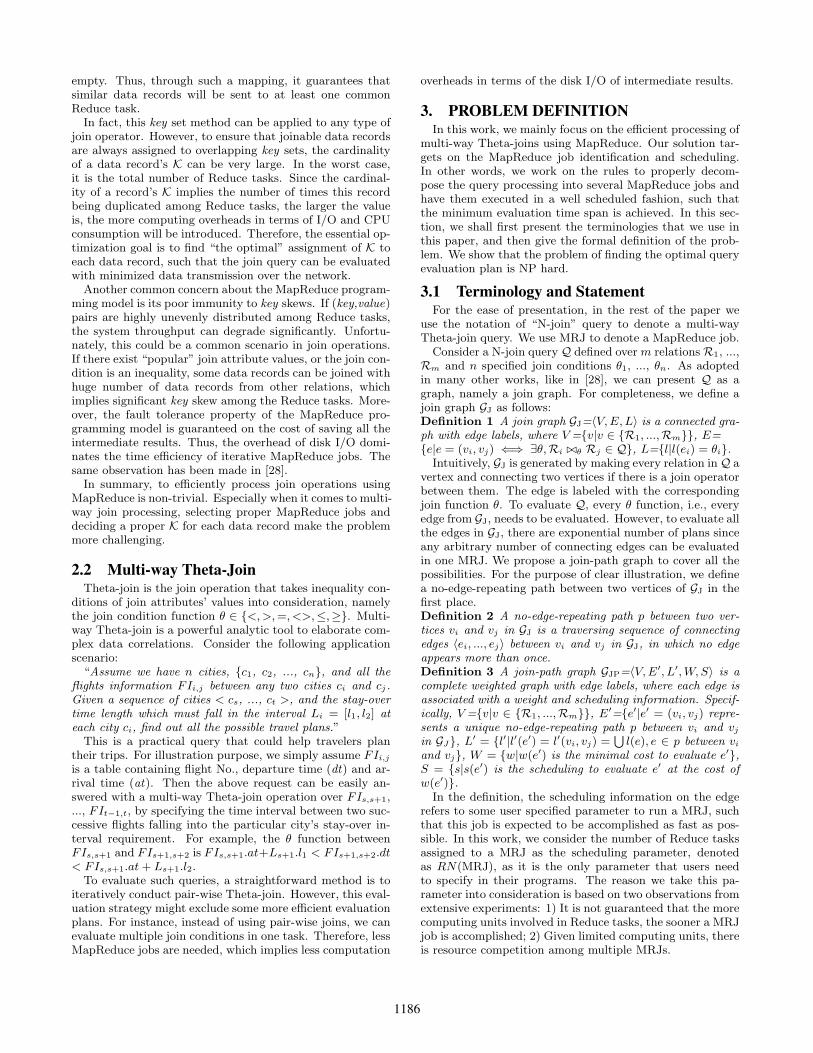
Intuitively, we enumerate all the possible join combina-tions in GJP. Note that in the context of join processing,Ri ⊲⊳ Rk ⊲⊳ Rj is the same with Rj ⊲⊳ Rk ⊲⊳ Ri, therefore,GJP is an undirected graph. We elaborate Definition 3.3 withthe following example. Given a join graph GJ, shown on theleft in Fig.1, a corresponding join-path graph GJP is gener-ated, which is presented in an adjacent matrix format on theright. The numbers enclosed in bracelets are the involved θ
functions on a path. For instance, in the cell correspondingto R1 and R2, {3, 4, 6, 5, 2} indicates a no-edge-repeatingpath {θ3, θ4, θ6, θ5, θ2} between R1 and R2. For this par-ticular example, notice that for every node there exists aclosed traversing path (or circuit) which covers all the edgesexactly once, namely the “Eulerian Circuit”. We use E(GJP)to denote a “Eulerian Circuit” of GJP in the figure. Sincewe only care what edges are involved in a path, any E(GJP)would be sufficient. Notice that in the figure, edge weightsand scheduling information are not presented. As a matterof fact, these information are incrementally computed dur-ing the generation of GJP, which will be illustrated in thelater Section.
R1 R3
R2 R4 R5
1
2
3 4
5
6
R1 R2 R3 R4 R5
R1{1,2,3} {1} {3,2}
{3,4,6,5,2}{3,4} {3,5,6}
{3} {1,2}
{1,2,4,6,5} {3,4,6,5}
{1,2,5} {1,2,4,6}
{3,5} {3,4,6}
R2 !{1,3,2}
{2,4} {2,5,6}
{1,3,4}
{1,3,5,6}
{2} {1,3}
{2,4,6,5}
{1,3,4,6,5}
{2,5} {2,4,6}
{1,3,5} {1,3,4,6}
R3 ! !{4,5,6}
{4} {6,5}
{4,3,1,2}
{6,5,3,1,2}
{6} {4,5}
{4,3,1,2,5}
R4 ! ! !{4,6,5}{3,1,2}
{5} {4,6}
{3,1,2,5}
{3,1,2,4,6}
R5 ! ! ! !{4,5,6}
)( JPG
)( JPG
)( JPG
)( JPG
)( JPG
Figure 1: Example join graph GJ and its correspond-
ing join-path graph GJP, presented in an adjacent
matrix
According to the definition of GJP, any edge e′ in GJP is acollection of connecting edges in GJ. Thus, e
′ in fact impliesa subgraph of GJ. As we use one MRJ to evaluate e′, denotedas MRJ(e′), GJP’s edge set represents all the possible MRJsthat can be employed to evaluate the original query Q. LetT denote a set of MRJs that are selected from GJP’s edge set.Intuitively, if the MRJs in T cover all the join conditions ofthe original query, we can answer the query by executing allthese MRJs. Formally, we define that T is “sufficient” asfollows:
Definition 4 T , a collection of MRJs, is sufficient to eval-uate Q iff
⋃
e′i = GJ.E, where MRJ(e′i)∈ T ,
Since it is trivial to check whether T is sufficient, for therest of this work, we only consider the case that T is suf-ficient. Thus, given T , we define its execution plan P as aspecific execution sequence of MRJs, which minimizes thetime span of using T to evaluate the original query Q. For-mally, we can define our problem as follows:Problem Definition: Given a N-join query Q and kP pro-cessing units, a join-path graph GJP according to Q’s joingraph GJ is built. We want to select a collection of edgesfrom GJP that correspondingly form a set of MRJs, denotedas Topt, such that there exists an execution plan P of Topt
which minimizes the query evaluation time.Obviously, there are many different choices of T to evalu-
ate Q. Moreover, given T and limited processing units, dif-ferent execution plans yield different evaluation time spans.In fact, the determination of P is non-trivial, we give thedetailed analysis of the hardness of our problem in the next
subsection. As we shall elaborate later, given T and kP avail-able processing units, we adopt an approximation method todetermine P in linear time.
3.2 Problem HardnessAccording to the problem definition, we need two steps to
find Topt: 1) generate GJP from GJ; 2) select MRJs for Topt.Neither one of these two steps is easy to solve.
For the first step, to construct GJP, we need to enumerateall the no-edge-repeating paths between any pair of verticesin GJ. Assume GJ has the “Eulerian trail”[16], which is away to traverse the graph with every edge be visited exactlyonce, then for any pair of vertices vi and vj , any differentno-edge-repeating path between them is a “sub-path” of anEulerian trail. If we know all the no-edge-repeating pathsbetween any pair of vertices, we can enumerate all the Eule-rian trails in polynomial time. Therefore, the complexity ofconstructing GJP is at least as hard as enumerating all theEulerian trails of a given graph, which is known to be #P-complete [6]. Moreover, we find that even GJ does not havean Eulerian trail, the problem complexity is not reduced atall, as we elaborate in the proof of the following theorem.
Theorem 1 Generating GJP from a given GJ is a #P com-plete problem.
Proof. If GJ has the Eulerian trail, constructing GJP is#P-complete (see the discussion above).On the contrary, if GJ does not have the Eulerian trail, it
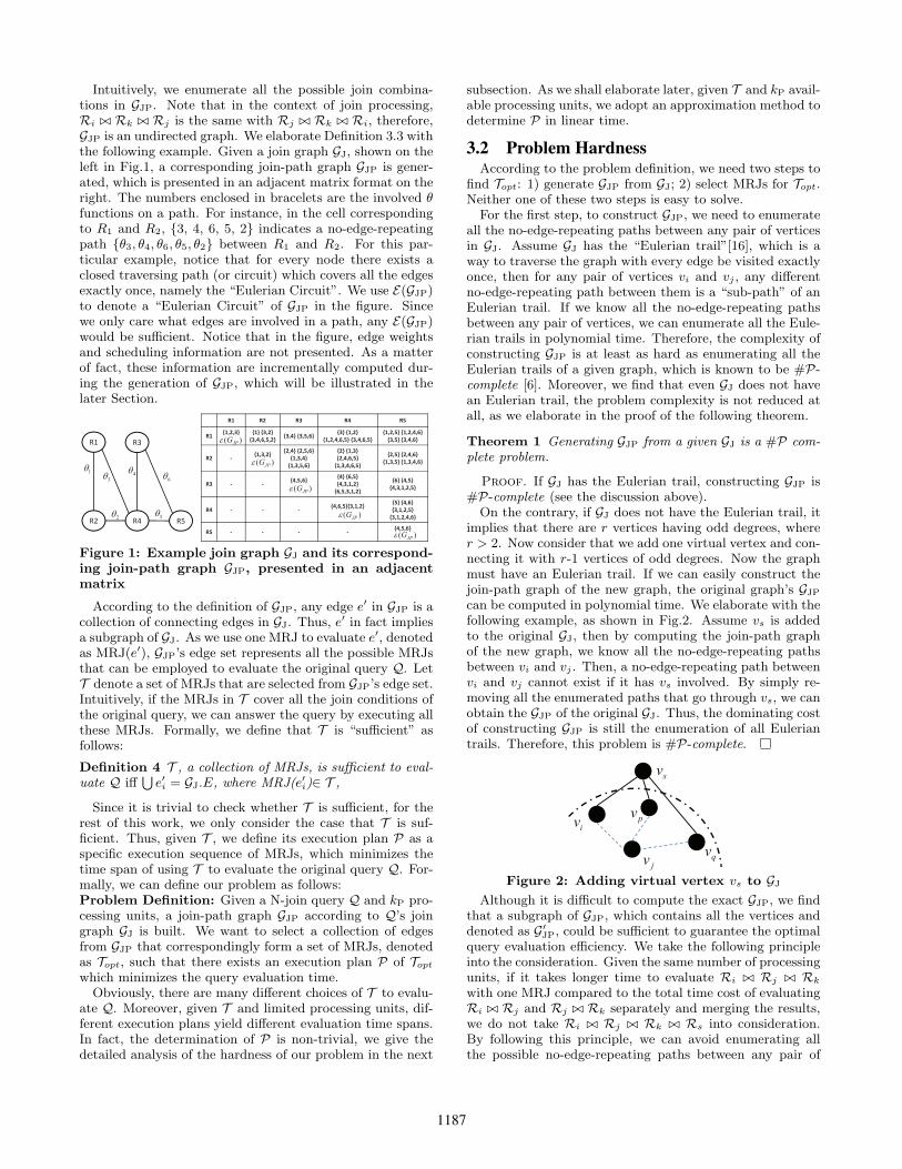
implies that there are r vertices having odd degrees, wherer > 2. Now consider that we add one virtual vertex and con-necting it with r-1 vertices of odd degrees. Now the graphmust have an Eulerian trail. If we can easily construct thejoin-path graph of the new graph, the original graph’s GJP
can be computed in polynomial time. We elaborate with thefollowing example, as shown in Fig.2. Assume vs is addedto the original GJ, then by computing the join-path graphof the new graph, we know all the no-edge-repeating pathsbetween vi and vj . Then, a no-edge-repeating path betweenvi and vj cannot exist if it has vs involved. By simply re-moving all the enumerated paths that go through vs, we canobtain the GJP of the original GJ. Thus, the dominating costof constructing GJP is still the enumeration of all Euleriantrails. Therefore, this problem is #P-complete.
sv
ivpv
qvjv
Figure 2: Adding virtual vertex vs to GJ
Although it is difficult to compute the exact GJP, we findthat a subgraph of GJP, which contains all the vertices anddenoted as G′
JP, could be sufficient to guarantee the optimalquery evaluation efficiency. We take the following principleinto the consideration. Given the same number of processingunits, if it takes longer time to evaluate Ri ⊲⊳ Rj ⊲⊳ Rk
with one MRJ compared to the total time cost of evaluatingRi ⊲⊳ Rj and Rj ⊲⊳ Rk separately and merging the results,we do not take Ri ⊲⊳ Rj ⊲⊳ Rk ⊲⊳ Rs into consideration.By following this principle, we can avoid enumerating allthe possible no-edge-repeating paths between any pair of
1187
vertices. As a matter of fact, we can obtain such a sufficientG′JP in polynomial time.The second step of our solution is to select the Topt. As-
sume the G′JP computed from the first step provides a col-
lection of edges, accordingly, we have a collection of MRJcandidates to evaluate the query. Although each edge inGJP is associated with a weight denoting the minimum timecost to evaluate all the join conditions contained in this edge,it is just an estimated time span on the condition that thereare enough processing units. However, when a T is chosen,and the number of processing units is limited, the time costof using T to answer Q need to be re-estimated. Assumewe can find the time cost estimation of T , denoted as C(T ),then the problem is to find such an optimal Topt from allpossible T s, which has the minimum time cost. Apparently,this is a variance of the classic set cover problem, which isknown to be NP hard [10]. Therefore, there are many heuris-tics and approximation algorithms can be adopted to solvethe selection problem.
As clearly indicated in the problem definition, the solutionlies in the construction of G′
JP and smartly select T based onthe cost estimation of a group of MRJs. Therefore, for therest of the paper, we shall first elaborate our cost models fora single MRJ and a group of MRJs. Then we present ourdetailed solution for the N-join query evaluation.
4. COST MODELTo highlight our observations on how much the overlap-
ping of computation and network cost would affect the ex-ecution of a MRJ, in this section we present a generalizedanalytical study on the execution time of both a single MRJand a group of MRJs. In the context of GJP constructionand T selection, we study the estimation of w(e′), wheree′ ∈ GJP.E, and C(T ), which is the time cost to evaluate T .
4.1 Estimating w(e′): Model for Single MRJSince our target is to find an optimal join plan, we only
consider the processing cost of join operations with MRJs.Generally, most of the CPU time for join processing is spenton simple comparison and counting, thus, system I/O costdominates the total execution time. For MapReduce jobs,heavy cost on large scale sequential disk scan and frequentI/O of intermediate results dominate the execution time.Therefore, we shall build a model for a MRJ’s executiontime based on the analysis of I/O and network cost.
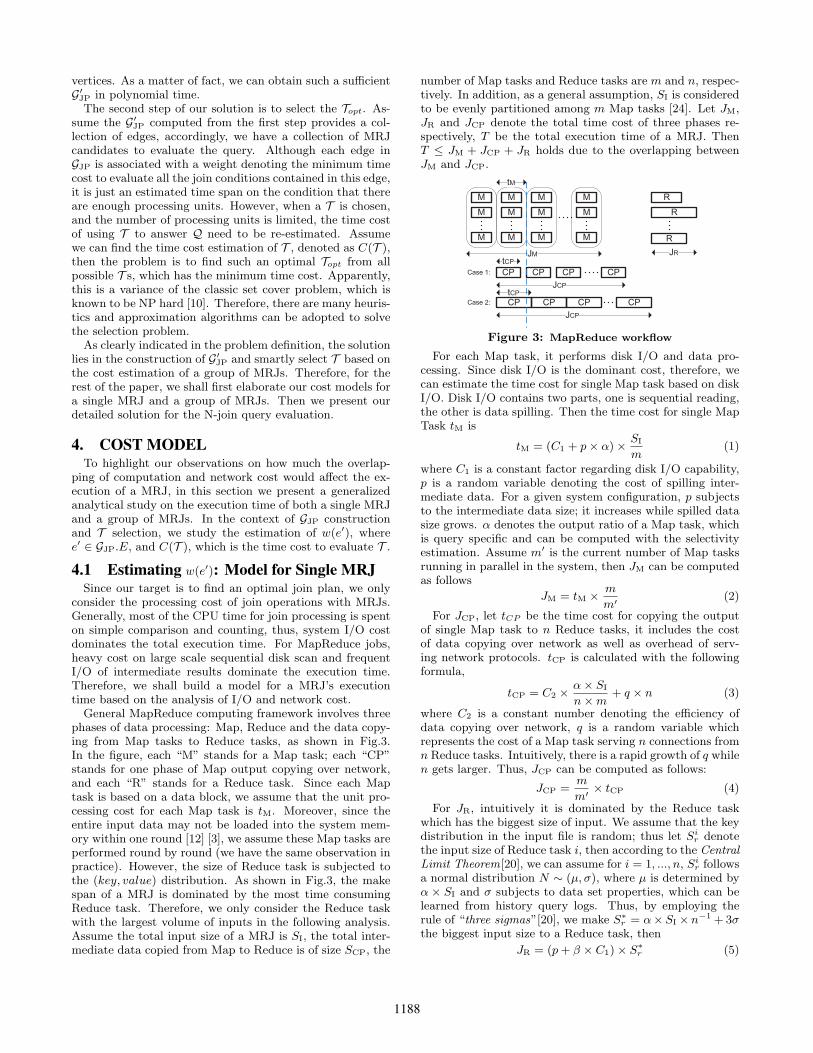
General MapReduce computing framework involves threephases of data processing: Map, Reduce and the data copy-ing from Map tasks to Reduce tasks, as shown in Fig.3.In the figure, each “M” stands for a Map task; each “CP”stands for one phase of Map output copying over network,and each “R” stands for a Reduce task. Since each Maptask is based on a data block, we assume that the unit pro-cessing cost for each Map task is tM. Moreover, since theentire input data may not be loaded into the system mem-ory within one round [12] [3], we assume these Map tasks areperformed round by round (we have the same observation inpractice). However, the size of Reduce task is subjected tothe (key, value) distribution. As shown in Fig.3, the makespan of a MRJ is dominated by the most time consumingReduce task. Therefore, we only consider the Reduce taskwith the largest volume of inputs in the following analysis.Assume the total input size of a MRJ is SI, the total inter-mediate data copied from Map to Reduce is of size SCP, the
number of Map tasks and Reduce tasks are m and n, respec-tively. In addition, as a general assumption, SI is consideredto be evenly partitioned among m Map tasks [24]. Let JM,JR and JCP denote the total time cost of three phases re-spectively, T be the total execution time of a MRJ. ThenT ≤ JM + JCP + JR holds due to the overlapping betweenJM and JCP.
tCP
M R
R
CP
M
M
M
M
M
M
M
M
CP CP
M
M
M
CP
CP CP CP CP
R
tM
JM
JCP
JCP
JR
tCP
Case 1:
Case 2:
Figure 3: MapReduce workflow
For each Map task, it performs disk I/O and data pro-cessing. Since disk I/O is the dominant cost, therefore, wecan estimate the time cost for single Map task based on diskI/O. Disk I/O contains two parts, one is sequential reading,the other is data spilling. Then the time cost for single MapTask tM is
tM = (C1 + p× α)×SI
m(1)
where C1 is a constant factor regarding disk I/O capability,p is a random variable denoting the cost of spilling inter-mediate data. For a given system configuration, p subjectsto the intermediate data size; it increases while spilled datasize grows. α denotes the output ratio of a Map task, whichis query specific and can be computed with the selectivityestimation. Assume m′ is the current number of Map tasksrunning in parallel in the system, then JM can be computedas follows
JM = tM ×m
m′(2)
For JCP, let tCP be the time cost for copying the outputof single Map task to n Reduce tasks, it includes the costof data copying over network as well as overhead of serv-ing network protocols. tCP is calculated with the followingformula,
tCP = C2 ×α× SI
n×m+ q × n (3)
where C2 is a constant number denoting the efficiency ofdata copying over network, q is a random variable whichrepresents the cost of a Map task serving n connections fromn Reduce tasks. Intuitively, there is a rapid growth of q whilen gets larger. Thus, JCP can be computed as follows:
JCP =m
m′× tCP (4)
For JR, intuitively it is dominated by the Reduce taskwhich has the biggest size of input. We assume that the keydistribution in the input file is random; thus let Si
r denotethe input size of Reduce task i, then according to the CentralLimit Theorem[20], we can assume for i = 1, ..., n, Si
r followsa normal distribution N ∼ (µ, σ), where µ is determined byα × SI and σ subjects to data set properties, which can belearned from history query logs. Thus, by employing therule of “three sigmas”[20], we make S∗
r = α× SI × n−1 +3σthe biggest input size to a Reduce task, then
JR = (p+ β × C1)× S∗r (5)
1188
where β is a query dependent variable denoting output ra-tio, which could be pre-computed based on the selectivityestimation.
Thus, the execution time T of a MRJ is:
T =
{
JM + tCP + JR if tM ≥ tCP
tM + JCP + JR if tM ≤ tCP(6)
In our cost model, parameters C1, C2, p and q are sys-tem dependent and need to be derived from observations onthe execution of real jobs, which are elaborated in the ex-periments section. This model favors MRJs that have I/Ocost dominate the execution time. Experiments show thatour method can produce a reasonable approximation of theMRJ running time in real practice.
4.2 Estimating C(T ): Model for A Group ofMRJs
There have been some works exploring the optimizationopportunity among multiple MRJs running in parallel, like[23] [24] and [28], by defining multiple types of correlationsamong MRJs. For instance, [23] defines “input correlation”,“transit correlation” and “job flow correlation”, targetingat the shared input scan and intermediate data partition.In fact, their techniques can be directly plugged into oursolution framework. Compared to these techniques, the sig-nificant difference of our study on the execution model of aset of MRJs is that our work takes the number of availableprocessing units into consideration. Therefore, the optimiza-tion problem we study here is orthogonal with the techniquesproposed in existing literatures that we mentioned above.
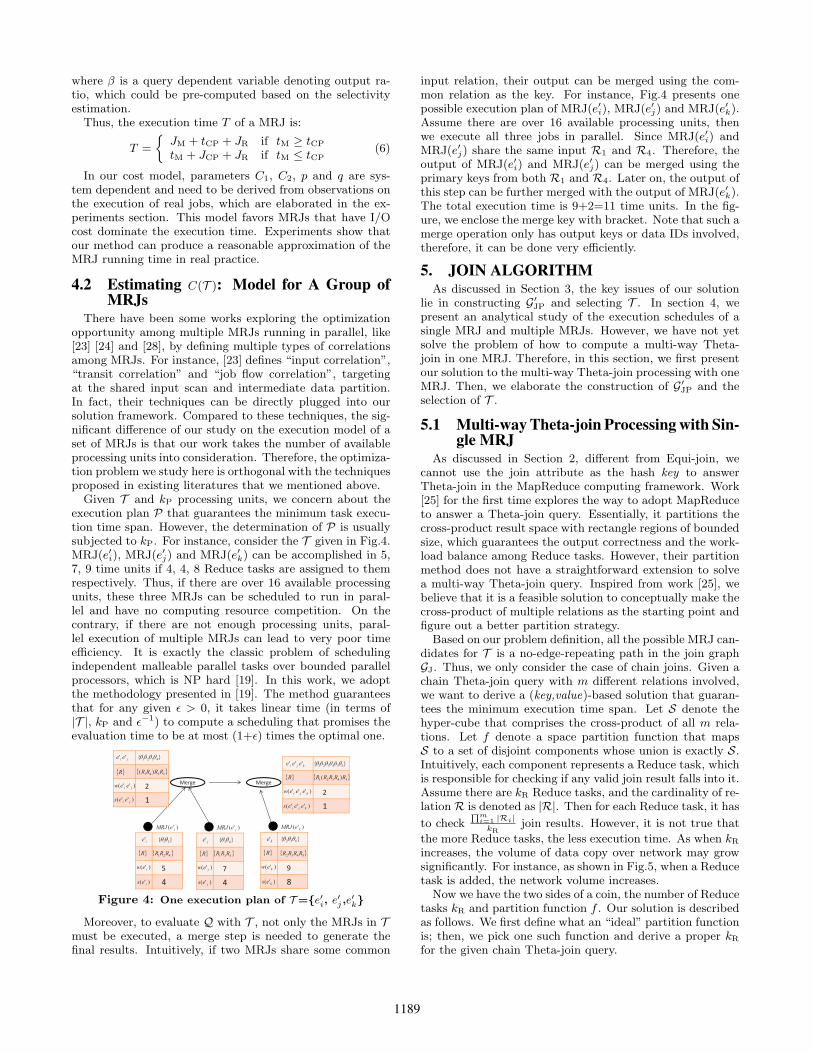
Given T and kP processing units, we concern about theexecution plan P that guarantees the minimum task execu-tion time span. However, the determination of P is usuallysubjected to kP. For instance, consider the T given in Fig.4.MRJ(e′i), MRJ(e′j) and MRJ(e′k) can be accomplished in 5,7, 9 time units if 4, 4, 8 Reduce tasks are assigned to themrespectively. Thus, if there are over 16 available processingunits, these three MRJs can be scheduled to run in paral-lel and have no computing resource competition. On thecontrary, if there are not enough processing units, paral-lel execution of multiple MRJs can lead to very poor timeefficiency. It is exactly the classic problem of schedulingindependent malleable parallel tasks over bounded parallelprocessors, which is NP hard [19]. In this work, we adoptthe methodology presented in [19]. The method guaranteesthat for any given ǫ > 0, it takes linear time (in terms of|T |, kP and ǫ−1) to compute a scheduling that promises theevaluation time to be at most (1+ǫ) times the optimal one.
5
4
}{ 21 ie'
)'( ieMRJ
!R
)'( iew
)'( ies
!421 RRR
7
4
}{ 43 je'
)'( jeMRJ
!R
)'( jew
)'( jes
!431 RRR
9
8
}{ 652 ke'
)'( keMRJ
!R
)'( kew
)'( kes
!5432 RRRR
Merge2
1
}{ 4321 ji ee ''
!R
)''( ji eew
)''( ji ees
!2341 )( RRRR
Merge
2
1
}{ 654321 kji eee '''
!R
)'''( kji eeew
)'''( kji eees
!54321 )( RRRRR
Figure 4: One execution plan of T ={e′i, e′j ,e
′k}
Moreover, to evaluate Q with T , not only the MRJs in Tmust be executed, a merge step is needed to generate thefinal results. Intuitively, if two MRJs share some common
input relation, their output can be merged using the com-mon relation as the key. For instance, Fig.4 presents onepossible execution plan of MRJ(e′i), MRJ(e′j) and MRJ(e′k).Assume there are over 16 available processing units, thenwe execute all three jobs in parallel. Since MRJ(e′i) andMRJ(e′j) share the same input R1 and R4. Therefore, theoutput of MRJ(e′i) and MRJ(e′j) can be merged using theprimary keys from both R1 and R4. Later on, the output ofthis step can be further merged with the output of MRJ(e′k).The total execution time is 9+2=11 time units. In the fig-ure, we enclose the merge key with bracket. Note that such amerge operation only has output keys or data IDs involved,therefore, it can be done very efficiently.
5. JOIN ALGORITHMAs discussed in Section 3, the key issues of our solution
lie in constructing G′JP and selecting T . In section 4, we
present an analytical study of the execution schedules of asingle MRJ and multiple MRJs. However, we have not yetsolve the problem of how to compute a multi-way Theta-join in one MRJ. Therefore, in this section, we first presentour solution to the multi-way Theta-join processing with oneMRJ. Then, we elaborate the construction of G′
JP and theselection of T .
5.1 Multi-way Theta-join Processing with Sin-gle MRJ
As discussed in Section 2, different from Equi-join, wecannot use the join attribute as the hash key to answerTheta-join in the MapReduce computing framework. Work[25] for the first time explores the way to adopt MapReduceto answer a Theta-join query. Essentially, it partitions thecross-product result space with rectangle regions of boundedsize, which guarantees the output correctness and the work-load balance among Reduce tasks. However, their partitionmethod does not have a straightforward extension to solvea multi-way Theta-join query. Inspired from work [25], webelieve that it is a feasible solution to conceptually make thecross-product of multiple relations as the starting point andfigure out a better partition strategy.
Based on our problem definition, all the possible MRJ can-didates for T is a no-edge-repeating path in the join graphGJ. Thus, we only consider the case of chain joins. Given achain Theta-join query with m different relations involved,we want to derive a (key,value)-based solution that guaran-tees the minimum execution time span. Let S denote thehyper-cube that comprises the cross-product of all m rela-tions. Let f denote a space partition function that mapsS to a set of disjoint components whose union is exactly S.Intuitively, each component represents a Reduce task, whichis responsible for checking if any valid join result falls into it.Assume there are kR Reduce tasks, and the cardinality of re-lation R is denoted as |R|. Then for each Reduce task, it has
to check∏m
i=1|Ri|
kRjoin results. However, it is not true that
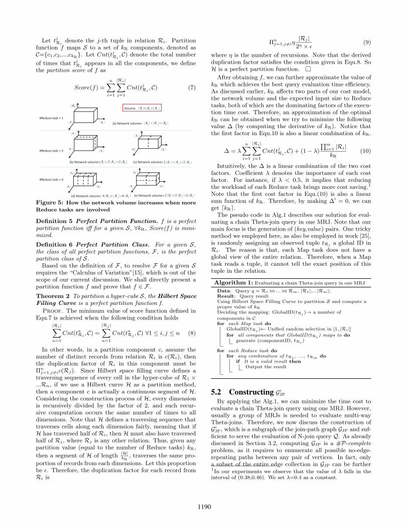
the more Reduce tasks, the less execution time. As when kRincreases, the volume of data copy over network may growsignificantly. For instance, as shown in Fig.5, when a Reducetask is added, the network volume increases.
Now we have the two sides of a coin, the number of Reducetasks kR and partition function f . Our solution is describedas follows. We first define what an “ideal” partition functionis; then, we pick one such function and derive a proper kRfor the given chain Theta-join query.
1189
Let tjRi
denote the j-th tuple in relation Ri. Partitionfunction f maps S to a set of kR components, denoted asC={c1,c2,...,ckR
}. Let Cnt(tjRi, C) denote the total number
of times that tjRi
appears in all the components, we definethe partition score of f as
Score(f) =
n∑
i=1
|Ri|∑
j=1
Cnt(tjRi, C) (7)
|| iR || jR
|| kR
|| iR|| jR
|| kR
|| iR || jR
|| kR
(a) Network volume= |||||| kji RRR
(b) Network volume= ||2||2|| kji RRR
(d) Network volume= ||4||||4 kji RRR
|| iR || jR
|| kR
(c) Network volume= ||2||||2 kji RRR
|| iR || jR
|| kR
(e) Network volume= ||2||2||2 kji RRR
#Reduce task = 1
#Reduce task = 2
#Reduce task = 4
|||||| jki RRR Assume
Figure 5: How the network volume increases when more
Reduce tasks are involved
Definition 5 Perfect Partition Function. f is a perfectpartition function iff for a given S, ∀kR, Score(f) is mini-mized.
Definition 6 Perfect Partition Class. For a given S,the class of all perfect partition functions, F , is the perfectpartition class of S.
Based on the definition of F , to resolve F for a given Srequires the “Calculus of Variation”[15], which is out of thescope of our current discussion. We shall directly present apartition function f and prove that f ∈ F .
Theorem 2 To partition a hyper-cube S, the Hilbert Space
Filling Curve is a perfect partition function f.
Proof. The minimum value of score function defined inEqu.7 is achieved when the following condition holds
|Ri|∑
u=1
Cnt(tuRi, C) =
|Rj |∑
u=1
Cnt(tuRj, C) ∀1 ≤ i, j ≤ n (8)
In other words, in a partition component c, assume thenumber of distinct records from relation Ri is c(Ri), thenthe duplication factor of Ri in this component must beΠn
j=1,j 6=ic(Rj). Since Hilbert space filling curve defines atraversing sequence of every cell in the hyper-cube of R1 ×...Rn, if we use a Hilbert curve H as a partition method,then a component c is actually a continuous segment of H.Considering the construction process of H, every dimensionis recursively divided by the factor of 2, and such recur-sive computation occurs the same number of times to alldimensions. Note that H defines a traversing sequence thattraverses cells along each dimension fairly, meaning that ifH has traversed half of Ri, then H must also have traversedhalf of Rj , where Rj is any other relation. Thus, given anypartition value (equal to the number of Reduce tasks) kR,
then a segment of H of length |H|kR
, traverses the same pro-
portion of records from each dimensions. Let this proportionbe ǫ. Therefore, the duplication factor for each record fromRi is
Πnj=1,j 6=iη
|Rj |
2η × ǫ(9)
where η is the number of recursions. Note that the derivedduplication factor satisfies the condition given in Equ.8. SoH is a perfect partition function.
After obtaining f , we can further approximate the value ofkR which achieves the best query evaluation time efficiency.As discussed earlier, kR affects two parts of our cost model,the network volume and the expected input size to Reducetasks, both of which are the dominating factors of the execu-tion time cost. Therefore, an approximation of the optimalkR can be obtained when we try to minimize the followingvalue ∆ (by computing the derivative of kR). Notice thatthe first factor in Equ.10 is also a linear combination of kR.
∆ = λ
n∑
i=1
|Ri|∑
j=1
Cnt(tjRi, C) + (1− λ)
∏m
i=1|Ri|
kR(10)
Intuitively, the ∆ is a linear combination of the two costfactors. Coefficient λ denotes the importance of each costfactor. For instance, if λ < 0.5, it implies that reducingthe workload of each Reduce task brings more cost saving.1
Note that the first cost factor in Equ.(10) is also a linearsum function of kR. Therefore, by making ∆′ = 0, we canget ⌈kR⌉.
The pseudo code in Alg.1 describes our solution for eval-uating a chain Theta-join query in one MRJ. Note that ourmain focus is the generation of (key,value) pairs. One trickymethod we employed here, as also be employed in work [25],is randomly assigning an observed tuple tRi
a global ID inRi. The reason is that, each Map task does not have aglobal view of the entire relation. Therefore, when a Maptask reads a tuple, it cannot tell the exact position of thistuple in the relation.
Algorithm 1: Evaluating a chain Theta-join query in one MRJ
Data: Query q = R1 ⊲⊳ ... ⊲⊳ Rm, |R1|,...|Rm|;Result: Query resultUsing Hilbert Space Filling Curve to partition S and compute aproper value of kR
Deciding the mapping: GlobalID(tRi)→ a number of
components in Cfor each Map task do
GlobalID(tRi)← Unified random selection in [1, |Ri|]
for all components that GlobalID(tRi) maps to do
generate (componentID, tRi)
for each Reduce task do
for any combination of tR1, ..., tRm do
if It is a valid result then
Output the result
5.2 Constructing G′JP
By applying the Alg.1, we can minimize the time cost toevaluate a chain Theta-join query using one MRJ. However,usually a group of MRJs is needed to evaluate multi-wayTheta-joins. Therefore, we now discuss the construction ofG′JP, which is a subgraph of the join-path graph GJP and suf-
ficient to serve the evaluation of N-join query Q. As alreadydiscussed in Section 3.2, computing GJP is a #P-completeproblem, as it requires to enumerate all possible no-edge-repeating paths between any pair of vertices. In fact, onlya subset of the entire edge collection in GJP can be further1In our experiments we observe that the value of λ falls in theinterval of (0.38,0.46). We set λ=0.4 as a constant.
1190
employed in Topt. Therefore, we propose two pruning con-ditions to effectively reduce the search space in this section.
The first intuition is that, to select Topt, the case thatmany join conditions are covered by multiple MRJs in Topt
is not preferred, because each join condition only needs tobe evaluated once. However, it does not imply that MRJs inTopt should strictly cover disjoint sets of join conditions. Be-cause sometimes, by including extra join conditions, the out-put volume of intermediate results can be reduced. There-fore, we exclude a MRJ(e′i) on the only condition that thereare other more efficient ways to evaluate all the join condi-tions that MRJ(e′i) covers. Formally, we state the pruningcondition in Lemma 1.
Lemma 1 Edge e′i should not be considered if there exists acollection of edges ES, and the following conditions are sat-isfied: 1) l′(e′j) ⊆
⋃
e′j∈ES l′(e′j); 2) w(e′i) > Maxe′
j∈ESw(e′j);
3) s(e′i) ≥∑
e′j∈ES s(e′j).
Lemma 1 is quite straightforward. If a MRJ can be sub-stituted with some other MRJs that cover at least the samenumber of join conditions and be evaluated more efficientlywith less demands on processing units, this MRJ cannot ap-pear in Topt. Because Topt is the optimal collection of MRJsto evaluate the query, containing any substitutable MRJmakes Topt sub-optimal. For the second pruning method,we present the following Lemma which further reduces thesearch space.
Lemma 2 Given two edges e′i and e′j , if e′i is not considered
and l′(e′i) ⊂ l′(e′j), then e′j should not be considered either.
Proof. Since e′i is not considered, it implies that thereis a better solution to cover l′(e′i)∩ l′(e′j). And this solutioncan be employed together with l′(e′j)− l′(e′i), which is moreefficient than computing l′(e′j) in one step. Therefore, l′(e′j)should not be considered.
Note that Lemma 2 is orthogonal to Lemma 1. SinceLemma 1 decides whether a MRJ should be considered asa member of Topt, if the answer is negative, we can em-ploy Lemma 2 to directly prune more undesired MRJs. Byemploying the two Lemmas proposed above, we develop analgorithm to construct G′
JP efficiently in an incremental man-ner, as presented in Alg.2.
Algorithm 2: Constructing G′
JP
Data: G′
Jcontaining n vertices and m edges, G′
JP= ∅, a sorted
list WL = ∅;Result: G′
JP
for i=1:n do
for j > i do
for L=1:m do
4 if there is a L-hop path from Ri to Rj then
e′ ← the L-hop path from Ri to Rj
if WL 6= ∅ then
scan WL to find the first group of edges thatcover e′
apply Lemma 1 to decide if report e′ to G′
JP
if e′ is not reported then
break //Lemma 2 plays the role
insert e′ into WL such that WL maintains asequence of edges in the ascending order ofw(e′)
Since we do not care the direction of a path, meaninge′(vi, vj)=e′(vj , vi), we compute the pair-wise join paths fol-lowing a fixed order of vertices (relations). In the Alg.2, we
employ the linear scan of a sorted list to help decide whethera path should be reported in G′
JP. One tricky part in the al-gorithm is line 4. A straightforward way is to employ DFSsearch from a given starting vertex, then the time complexityis O(m + n). However, it introduces much redundant workfor every vertex to perform this task. A better solution is be-fore we run Alg.2, we firstly traverse GJ once and record theL-hop neighbor of every vertex. It takes only O(m+n) timecomplexity. Then, line 4 can be determined in O(1) time.Overall, we can see the worst time complexity of Alg.2 isO(n2m). This happens only when GJ is a complete graph.In real practice, due to the sparsity of the graph, Alg.2 isquick enough to generate GJP for a given GJ. As observed inthe experiments, G′
JP can be generated in the time frame ofhundreds of microseconds.
After G′JP is obtained, we select Topt following the method-
ology presented in [14], which gives O(ln(n)) approximationratio of the optimum.
6. EXPERIMENTSTo verify the effectiveness of our solution, we conduct ex-
periments on a real cluster environment with both real andsynthetic data sets. In this section, we first describe thesetup configuration of the test-bed and the data sets weused. Then we validate our cost model. We compare oursolution for multi-way Theta-join processing with YSmart[23], Hive and Pig. We demonstrate that our solution cansave on average 30% of query processing time when com-pared to the state of art methods. Especially in the cases ofcomplex queries over huge volume of data, our method cansave up to 150% of evaluation time.
6.1 Experiments SetupOur experiments run exclusively on a 13-node cluster,
where one node serves as the master node (Namenode). Ev-ery node has 2× Intel(R) Core(TM) i7 CPU 950 and 2×Kingston DDR-3 1333MHz 4GB of memory, 2.5TB HHD at-tached, running 2.6.35-22-server #35-Ubuntu SMP. All thenodes are connected with a 10GB-switch. In total, the testbed has 104 cores, 104GB main memory, and over 25TBstorage capacity.
Parameter Name Default Setfs.bloksize 64MB 64MBio.sort.mb 100M 512MB
io.sort.record.percentage 0.05 0.1io.sort.spill.percentage 0.8 0.9
io.sort.factor 100 300dfs.replication 3 3
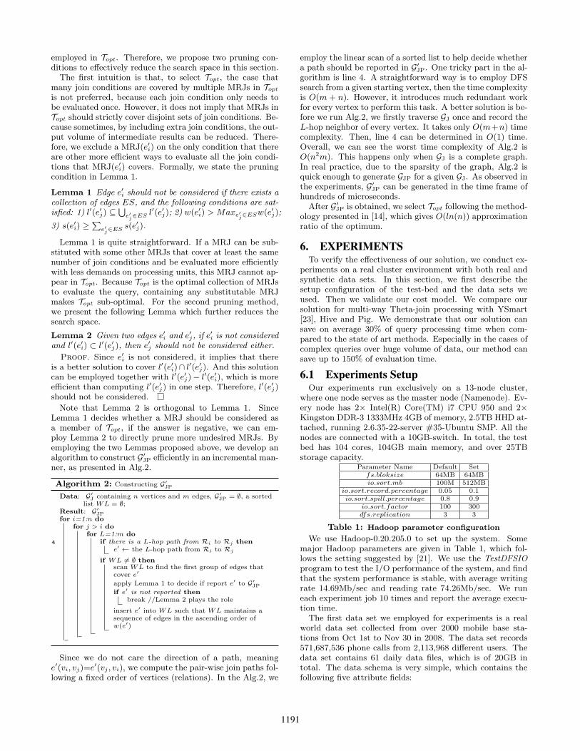
Table 1: Hadoop parameter configuration
We use Hadoop-0.20.205.0 to set up the system. Somemajor Hadoop parameters are given in Table 1, which fol-lows the setting suggested by [21]. We use the TestDFSIOprogram to test the I/O performance of the system, and findthat the system performance is stable, with average writingrate 14.69Mb/sec and reading rate 74.26Mb/sec. We runeach experiment job 10 times and report the average execu-tion time.
The first data set we employed for experiments is a realworld data set collected from over 2000 mobile base sta-tions from Oct 1st to Nov 30 in 2008. The data set records571,687,536 phone calls from 2,113,968 different users. Thedata set contains 61 daily data files, which is of 20GB intotal. The data schema is very simple, which contains thefollowing five attribute fields:
1191
1600
1800
2000
2200
2400
2600
2800
3000
0 10 20 30 40 50 60 70
Load Time (Sec)
Data Set Volume
(a) Input Size: 500GB
116
118
120
122
124
126
128
130
0 10 20 30 40 50 60 70
Load Time (Sec)
Data Set Volume
(b) Input Size: 100GB
35
40
45
50
55
60
0 10 20 30 40 50 60 70
Load Time (Sec)
Data Set Volume
(c) Input Size: 10GB
28
30
32
34
36
38
40
42
44
46
48
50
0 10 20 30 40 50 60 70
Load Time (Sec)
Data Set Volume
(d) Input Size: 1GB
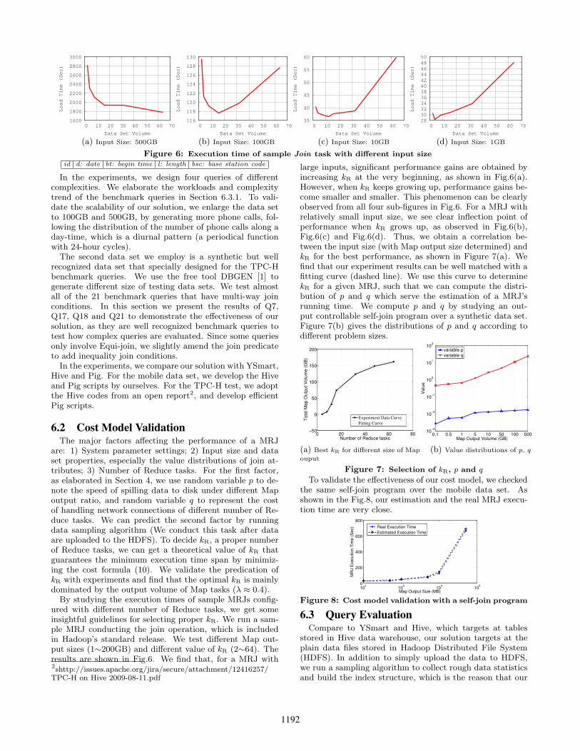
Figure 6: Execution time of sample Join task with different input size
id d: date bt: begin time l: length bsc: base station code
In the experiments, we design four queries of differentcomplexities. We elaborate the workloads and complexitytrend of the benchmark queries in Section 6.3.1. To vali-date the scalability of our solution, we enlarge the data setto 100GB and 500GB, by generating more phone calls, fol-lowing the distribution of the number of phone calls along aday-time, which is a diurnal pattern (a periodical functionwith 24-hour cycles).
The second data set we employ is a synthetic but wellrecognized data set that specially designed for the TPC-Hbenchmark queries. We use the free tool DBGEN [1] togenerate different size of testing data sets. We test almostall of the 21 benchmark queries that have multi-way joinconditions. In this section we present the results of Q7,Q17, Q18 and Q21 to demonstrate the effectiveness of oursolution, as they are well recognized benchmark queries totest how complex queries are evaluated. Since some queriesonly involve Equi-join, we slightly amend the join predicateto add inequality join conditions.
In the experiments, we compare our solution with YSmart,Hive and Pig. For the mobile data set, we develop the Hiveand Pig scripts by ourselves. For the TPC-H test, we adoptthe Hive codes from an open report2, and develop efficientPig scripts.
6.2 Cost Model ValidationThe major factors affecting the performance of a MRJ
are: 1) System parameter settings; 2) Input size and dataset properties, especially the value distributions of join at-tributes; 3) Number of Reduce tasks. For the first factor,as elaborated in Section 4, we use random variable p to de-note the speed of spilling data to disk under different Mapoutput ratio, and random variable q to represent the costof handling network connections of different number of Re-duce tasks. We can predict the second factor by runningdata sampling algorithm (We conduct this task after dataare uploaded to the HDFS). To decide kR, a proper numberof Reduce tasks, we can get a theoretical value of kR thatguarantees the minimum execution time span by minimiz-ing the cost formula (10). We validate the predication ofkR with experiments and find that the optimal kR is mainlydominated by the output volume of Map tasks (λ ≈ 0.4).
By studying the execution times of sample MRJs config-ured with different number of Reduce tasks, we get someinsightful guidelines for selecting proper kR. We run a sam-ple MRJ conducting the join operation, which is includedin Hadoop’s standard release. We test different Map out-put sizes (1∼200GB) and different value of kR (2∼64). Theresults are shown in Fig.6. We find that, for a MRJ with2shttp://issues.apache.org/jira/secure/attachment/12416257/TPC-H on Hive 2009-08-11.pdf
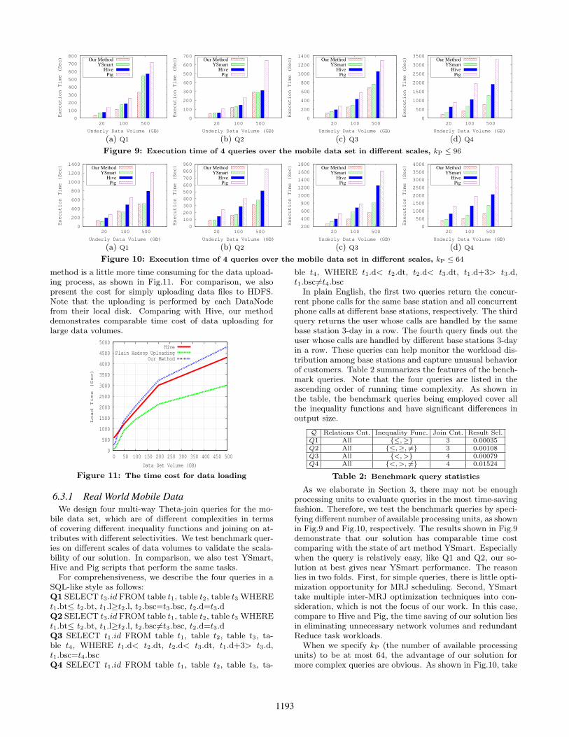
large inputs, significant performance gains are obtained byincreasing kR at the very beginning, as shown in Fig.6(a).However, when kR keeps growing up, performance gains be-come smaller and smaller. This phenomenon can be clearlyobserved from all four sub-figures in Fig.6. For a MRJ withrelatively small input size, we see clear inflection point ofperformance when kR grows up, as observed in Fig.6(b),Fig.6(c) and Fig.6(d). Thus, we obtain a correlation be-tween the input size (with Map output size determined) andkR for the best performance, as shown in Figure 7(a). Wefind that our experiment results can be well matched with afitting curve (dashed line). We use this curve to determinekR for a given MRJ, such that we can compute the distri-bution of p and q which serve the estimation of a MRJ’srunning time. We compute p and q by studying an out-put controllable self-join program over a synthetic data set.Figure 7(b) gives the distributions of p and q according todifferent problem sizes.
0 20 40 60 80−50
0
50
100
150
200
Number of Reduce tasks
Tota
l M
ap O
utp
ut V
olu
me (
GB
)
Experiment Data Curve
Fitting Curve
(a) Best kR for different size of Map
ouput
0.1 0.5 1 5 10 50 100 50010
−3
10−2
10−1
100
101
102
Map Output Volume (GB)
Valu
e
variable pvariable q
(b) Value distributions of p, q
Figure 7: Selection of kR, p and q
To validate the effectiveness of our cost model, we checkedthe same self-join program over the mobile data set. Asshown in the Fig.8, our estimation and the real MRJ execu-tion time are very close.
102
103
104
105
0
200
400
600
800
Map Output Size (MB)
MR
J E
xecution T
ime (
Sec)
Real Execution Time
Estimated Execution Time
Figure 8: Cost model validation with a self-join program
6.3 Query EvaluationCompare to YSmart and Hive, which targets at tables
stored in Hive data warehouse, our solution targets at theplain data files stored in Hadoop Distributed File System(HDFS). In addition to simply upload the data to HDFS,we run a sampling algorithm to collect rough data statisticsand build the index structure, which is the reason that our
1192
0
100
200
300
400
500
600
700
800
20 100 500
Execution Time (Sec)
Underly Data Volume (GB)
Our MethodYSmart
HivePig
(a) Q1
0
100
200
300
400
500
600
700
20 100 500
Execution Time (Sec)
Underly Data Volume (GB)
Our MethodYSmart
HivePig
(b) Q2
0
200
400
600
800
1000
1200
1400
20 100 500
Execution Time (Sec)
Underly Data Volume (GB)
Our MethodYSmart
HivePig
(c) Q3
0
500
1000
1500
2000
2500
3000
3500
20 100 500
Execution Time (Sec)
Underly Data Volume (GB)
Our MethodYSmart
HivePig
(d) Q4
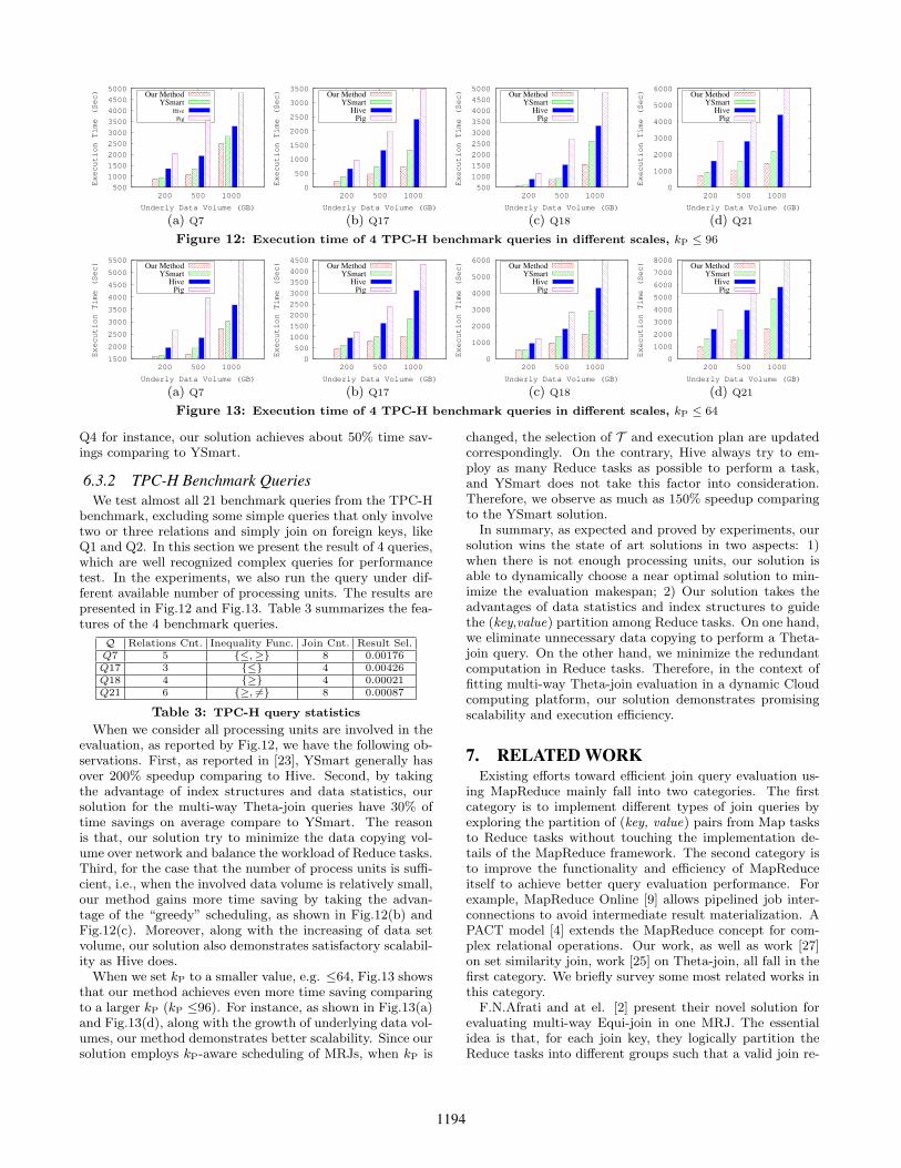
Figure 9: Execution time of 4 queries over the mobile data set in different scales, kP ≤ 96
0
200
400
600
800
1000
1200
1400
20 100 500
Execution Time (Sec)
Underly Data Volume (GB)
Our MethodYSmart
HivePig
(a) Q1
0
100
200
300
400
500
600
700
800
900
20 100 500
Execution Time (Sec)
Underly Data Volume (GB)
Our MethodYSmart
HivePig
(b) Q2
200
400
600
800
1000
1200
1400
1600
1800
20 100 500
Execution Time (Sec)
Underly Data Volume (GB)
Our MethodYSmart
HivePig
(c) Q3
0
500
1000
1500
2000
2500
3000
3500
4000
20 100 500
Execution Time (Sec)
Underly Data Volume (GB)
Our MethodYSmart
HivePig
(d) Q4
Figure 10: Execution time of 4 queries over the mobile data set in different scales, kP ≤ 64
method is a little more time consuming for the data upload-ing process, as shown in Fig.11. For comparison, we alsopresent the cost for simply uploading data files to HDFS.Note that the uploading is performed by each DataNodefrom their local disk. Comparing with Hive, our methoddemonstrates comparable time cost of data uploading forlarge data volumes.
0
500
1000
1500
2000
2500
3000
3500
4000
4500
5000
0 50 100 150 200 250 300 350 400 450 500
Load Time (Sec)
Data Set Volume (GB)
HivePlain Hadoop Uploading
Our Method
Figure 11: The time cost for data loading
6.3.1 Real World Mobile Data
We design four multi-way Theta-join queries for the mo-bile data set, which are of different complexities in termsof covering different inequality functions and joining on at-tributes with different selectivities. We test benchmark quer-ies on different scales of data volumes to validate the scala-bility of our solution. In comparison, we also test YSmart,Hive and Pig scripts that perform the same tasks.
For comprehensiveness, we describe the four queries in aSQL-like style as follows:Q1 SELECT t3.id FROM table t1, table t2, table t3 WHEREt1.bt≤ t2.bt, t1.l≥t2.l, t2.bsc=t3.bsc, t2.d=t3.dQ2 SELECT t3.id FROM table t1, table t2, table t3 WHEREt1.bt≤ t2.bt, t1.l≥t2.l, t2.bsc 6=t3.bsc, t2.d=t3.dQ3 SELECT t1.id FROM table t1, table t2, table t3, ta-ble t4, WHERE t1.d< t2.dt, t2.d< t3.dt, t1.d+3> t3.d,t1.bsc=t4.bscQ4 SELECT t1.id FROM table t1, table t2, table t3, ta-
ble t4, WHERE t1.d< t2.dt, t2.d< t3.dt, t1.d+3> t3.d,t1.bsc 6=t4.bsc
In plain English, the first two queries return the concur-rent phone calls for the same base station and all concurrentphone calls at different base stations, respectively. The thirdquery returns the user whose calls are handled by the samebase station 3-day in a row. The fourth query finds out theuser whose calls are handled by different base stations 3-dayin a row. These queries can help monitor the workload dis-tribution among base stations and capture unusual behaviorof customers. Table 2 summarizes the features of the bench-mark queries. Note that the four queries are listed in theascending order of running time complexity. As shown inthe table, the benchmark queries being employed cover allthe inequality functions and have significant differences inoutput size.
Q Relations Cnt. Inequality Func. Join Cnt. Result Sel.Q1 All {≤,≥} 3 0.00035Q2 All {≤,≥, 6=} 3 0.00108Q3 All {<,>} 4 0.00079Q4 All {<,>, 6=} 4 0.01524
Table 2: Benchmark query statistics
As we elaborate in Section 3, there may not be enoughprocessing units to evaluate queries in the most time-savingfashion. Therefore, we test the benchmark queries by speci-fying different number of available processing units, as shownin Fig.9 and Fig.10, respectively. The results shown in Fig.9demonstrate that our solution has comparable time costcomparing with the state of art method YSmart. Especiallywhen the query is relatively easy, like Q1 and Q2, our so-lution at best gives near YSmart performance. The reasonlies in two folds. First, for simple queries, there is little opti-mization opportunity for MRJ scheduling. Second, YSmarttake multiple inter-MRJ optimization techniques into con-sideration, which is not the focus of our work. In this case,compare to Hive and Pig, the time saving of our solution liesin eliminating unnecessary network volumes and redundantReduce task workloads.
When we specify kP (the number of available processingunits) to be at most 64, the advantage of our solution formore complex queries are obvious. As shown in Fig.10, take
1193
500
1000
1500
2000
2500
3000
3500
4000
4500
5000
200 500 1000
Execution Time (Sec)
Underly Data Volume (GB)
Our MethodYSmart
Hive
Pig
(a) Q7
0
500
1000
1500
2000
2500
3000
3500
200 500 1000
Execution Time (Sec)
Underly Data Volume (GB)
Our MethodYSmart
HivePig
(b) Q17
500
1000
1500
2000
2500
3000
3500
4000
4500
5000
200 500 1000
Execution Time (Sec)
Underly Data Volume (GB)
Our MethodYSmart
HivePig
(c) Q18
0
1000
2000
3000
4000
5000
6000
200 500 1000
Execution Time (Sec)
Underly Data Volume (GB)
Our MethodYSmart
HivePig
(d) Q21
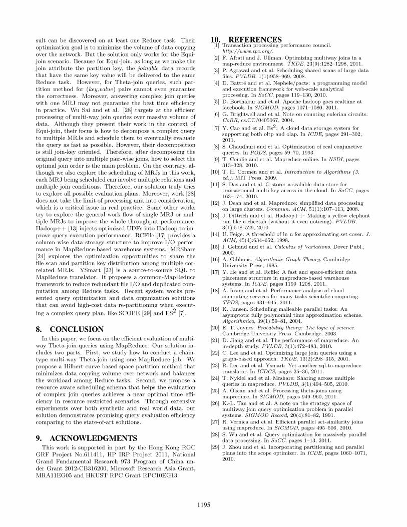
Figure 12: Execution time of 4 TPC-H benchmark queries in different scales, kP ≤ 96
1500
2000
2500
3000
3500
4000
4500
5000
5500
200 500 1000
Execution Time (Sec)
Underly Data Volume (GB)
Our MethodYSmart
HivePig
(a) Q7
0
500
1000
1500
2000
2500
3000
3500
4000
4500
200 500 1000
Execution Time (Sec)
Underly Data Volume (GB)
Our MethodYSmart
HivePig
(b) Q17
0
1000
2000
3000
4000
5000
6000
200 500 1000
Execution Time (Sec)
Underly Data Volume (GB)
Our MethodYSmart
HivePig
(c) Q18
0
1000
2000
3000
4000
5000
6000
7000
8000
200 500 1000
Execution Time (Sec)
Underly Data Volume (GB)
Our MethodYSmart
HivePig
(d) Q21
Figure 13: Execution time of 4 TPC-H benchmark queries in different scales, kP ≤ 64
Q4 for instance, our solution achieves about 50% time sav-ings comparing to YSmart.
6.3.2 TPC-H Benchmark Queries
We test almost all 21 benchmark queries from the TPC-Hbenchmark, excluding some simple queries that only involvetwo or three relations and simply join on foreign keys, likeQ1 and Q2. In this section we present the result of 4 queries,which are well recognized complex queries for performancetest. In the experiments, we also run the query under dif-ferent available number of processing units. The results arepresented in Fig.12 and Fig.13. Table 3 summarizes the fea-tures of the 4 benchmark queries.
Q Relations Cnt. Inequality Func. Join Cnt. Result Sel.Q7 5 {≤,≥} 8 0.00176Q17 3 {≤} 4 0.00426Q18 4 {≥} 4 0.00021Q21 6 {≥, 6=} 8 0.00087
Table 3: TPC-H query statistics
When we consider all processing units are involved in theevaluation, as reported by Fig.12, we have the following ob-servations. First, as reported in [23], YSmart generally hasover 200% speedup comparing to Hive. Second, by takingthe advantage of index structures and data statistics, oursolution for the multi-way Theta-join queries have 30% oftime savings on average compare to YSmart. The reasonis that, our solution try to minimize the data copying vol-ume over network and balance the workload of Reduce tasks.Third, for the case that the number of process units is suffi-cient, i.e., when the involved data volume is relatively small,our method gains more time saving by taking the advan-tage of the “greedy” scheduling, as shown in Fig.12(b) andFig.12(c). Moreover, along with the increasing of data setvolume, our solution also demonstrates satisfactory scalabil-ity as Hive does.
When we set kP to a smaller value, e.g. ≤64, Fig.13 showsthat our method achieves even more time saving comparingto a larger kP (kP ≤96). For instance, as shown in Fig.13(a)and Fig.13(d), along with the growth of underlying data vol-umes, our method demonstrates better scalability. Since oursolution employs kP-aware scheduling of MRJs, when kP is
changed, the selection of T and execution plan are updatedcorrespondingly. On the contrary, Hive always try to em-ploy as many Reduce tasks as possible to perform a task,and YSmart does not take this factor into consideration.Therefore, we observe as much as 150% speedup comparingto the YSmart solution.
In summary, as expected and proved by experiments, oursolution wins the state of art solutions in two aspects: 1)when there is not enough processing units, our solution isable to dynamically choose a near optimal solution to min-imize the evaluation makespan; 2) Our solution takes theadvantages of data statistics and index structures to guidethe (key,value) partition among Reduce tasks. On one hand,we eliminate unnecessary data copying to perform a Theta-join query. On the other hand, we minimize the redundantcomputation in Reduce tasks. Therefore, in the context offitting multi-way Theta-join evaluation in a dynamic Cloudcomputing platform, our solution demonstrates promisingscalability and execution efficiency.
7. RELATED WORKExisting efforts toward efficient join query evaluation us-
ing MapReduce mainly fall into two categories. The firstcategory is to implement different types of join queries byexploring the partition of (key, value) pairs from Map tasksto Reduce tasks without touching the implementation de-tails of the MapReduce framework. The second category isto improve the functionality and efficiency of MapReduceitself to achieve better query evaluation performance. Forexample, MapReduce Online [9] allows pipelined job inter-connections to avoid intermediate result materialization. APACT model [4] extends the MapReduce concept for com-plex relational operations. Our work, as well as work [27]on set similarity join, work [25] on Theta-join, all fall in thefirst category. We briefly survey some most related works inthis category.
F.N.Afrati and at el. [2] present their novel solution forevaluating multi-way Equi-join in one MRJ. The essentialidea is that, for each join key, they logically partition theReduce tasks into different groups such that a valid join re-
1194
sult can be discovered on at least one Reduce task. Theiroptimization goal is to minimize the volume of data copyingover the network. But the solution only works for the Equi-join scenario. Because for Equi-join, as long as we make thejoin attribute the partition key, the joinable data recordsthat have the same key value will be delivered to the sameReduce task. However, for Theta-join queries, such par-tition method for (key,value) pairs cannot even guaranteethe correctness. Moreover, answering complex join querieswith one MRJ may not guarantee the best time efficiencyin practice. Wu Sai and et al. [28] targets at the efficientprocessing of multi-way join queries over massive volume ofdata. Although they present their work in the context ofEqui-join, their focus is how to decompose a complex queryto multiple MRJs and schedule them to eventually evaluatethe query as fast as possible. However, their decompositionis still join-key oriented. Therefore, after decomposing theoriginal query into multiple pair-wise joins, how to select theoptimal join order is the main problem. On the contrary, al-though we also explore the scheduling of MRJs in this work,each MRJ being scheduled can involve multiple relations andmultiple join conditions. Therefore, our solution truly triesto explore all possible evaluation plans. Moreover, work [28]does not take the limit of processing unit into consideration,which is a critical issue in real practice. Some other workstry to explore the general work flow of single MRJ or mul-tiple MRJs to improve the whole throughput performance.Hadoop++ [13] injects optimized UDFs into Hadoop to im-prove query execution performance. RCFile [17] provides acolumn-wise data storage structure to improve I/O perfor-mance in MapReduce-based warehouse systems. MRShare[24] explores the optimization opportunities to share thefile scan and partition key distribution among multiple cor-related MRJs. YSmart [23] is a source-to-source SQL toMapReduce translator. It proposes a common-MapReduceframework to reduce redundant file I/O and duplicated com-putation among Reduce tasks. Recent system works pre-sented query optimization and data organization solutionsthat can avoid high-cost data re-partitioning when execut-
ing a complex query plan, like SCOPE [29] and ES2 [7].
8. CONCLUSIONIn this paper, we focus on the efficient evaluation of multi-
way Theta-join queries using MapReduce. Our solution in-cludes two parts. First, we study how to conduct a chain-type multi-way Theta-join using one MapReduce job. Wepropose a Hilbert curve based space partition method thatminimizes data copying volume over network and balancesthe workload among Reduce tasks. Second, we propose aresource aware scheduling schema that helps the evaluationof complex join queries achieves a near optimal time effi-ciency in resource restricted scenarios. Through extensiveexperiments over both synthetic and real world data, oursolution demonstrates promising query evaluation efficiencycomparing to the state-of-art solutions.
9. ACKNOWLEDGMENTSThis work is supported in part by the Hong Kong RGC
GRF Project No.611411, HP IRP Project 2011, NationalGrand Fundamental Research 973 Program of China un-der Grant 2012-CB316200, Microsoft Research Asia Grant,MRA11EG05 and HKUST RPC Grant RPC10EG13.
10. REFERENCES[1] Transaction processing performance council.
http://www.tpc.org/.
[2] F. Afrati and J. Ullman. Optimizing multiway joins in amap-reduce environment. TKDE, 23(9):1282–1298, 2011.
[3] P. Agrawal and et al. Scheduling shared scans of large datafiles. PVLDB, 1(1):958–969, 2008.
[4] D. Battre and et al. Nephele/pacts: a programming modeland execution framework for web-scale analyticalprocessing. In SoCC, pages 119–130, 2010.
[5] D. Borthakur and et al. Apache hadoop goes realtime atfacebook. In SIGMOD, pages 1071–1080, 2011.
[6] G. Brightwell and et al. Note on counting eulerian circuits.CoRR, cs.CC/0405067, 2004.
[7] Y. Cao and et al. Es2: A cloud data storage system forsupporting both oltp and olap. In ICDE, pages 291–302,2011.
[8] S. Chaudhuri and et al. Optimization of real conjunctivequeries. In PODS, pages 59–70, 1993.
[9] T. Condie and et al. Mapreduce online. In NSDI, pages313–328, 2010.
[10] T. H. Cormen and et al. Introduction to Algorithms (3.ed.). MIT Press, 2009.
[11] S. Das and et al. G-store: a scalable data store fortransactional multi key access in the cloud. In SoCC, pages163–174, 2010.
[12] J. Dean and et al. Mapreduce: simplified data processingon large clusters. Commun. ACM, 51(1):107–113, 2008.
[13] J. Dittrich and et al. Hadoop++: Making a yellow elephantrun like a cheetah (without it even noticing). PVLDB,3(1):518–529, 2010.
[14] U. Feige. A threshold of ln n for approximating set cover. J.ACM, 45(4):634–652, 1998.
[15] I. Gelfand and et al. Calculus of Variations. Dover Publ.,2000.
[16] A. Gibbons. Algorithmic Graph Theory. CambridgeUniversity Press, 1985.
[17] Y. He and et al. Rcfile: A fast and space-efficient dataplacement structure in mapreduce-based warehousesystems. In ICDE, pages 1199–1208, 2011.
[18] A. Iosup and et al. Performance analysis of cloudcomputing services for many-tasks scientific computing.TPDS, pages 931–945, 2011.
[19] K. Jansen. Scheduling malleable parallel tasks: Anasymptotic fully polynomial time approximation scheme.Algorithmica, 39(1):59–81, 2004.
[20] E. T. Jaynes. Probability theory: The logic of science.Cambridge University Press, Cambridge, 2003.
[21] D. Jiang and et al. The performance of mapreduce: Anin-depth study. PVLDB, 3(1):472–483, 2010.
[22] C. Lee and et al. Optimizing large join queries using agraph-based approach. TKDE, 13(2):298–315, 2001.
[23] R. Lee and et al. Ysmart: Yet another sql-to-mapreducetranslator. In ICDCS, pages 25–36, 2011.
[24] T. Nykiel and et al. Mrshare: Sharing across multiplequeries in mapreduce. PVLDB, 3(1):494–505, 2010.
[25] A. Okcan and et al. Processing theta-joins usingmapreduce. In SIGMOD, pages 949–960, 2011.
[26] K.-L. Tan and et al. A note on the strategy space ofmultiway join query optimization problem in parallelsystems. SIGMOD Record, 20(4):81–82, 1991.
[27] R. Vernica and et al. Efficient parallel set-similarity joinsusing mapreduce. In SIGMOD, pages 495–506, 2010.
[28] S. Wu and et al. Query optimization for massively paralleldata processing. In SoCC, pages 1–13, 2011.
[29] J. Zhou and et al. Incorporating partitioning and parallelplans into the scope optimizer. In ICDE, pages 1060–1071,2010.
1195