effects of cyclic prefix jamming versus noise jamming in
TRANSCRIPT
Air Force Institute of Technology Air Force Institute of Technology
AFIT Scholar AFIT Scholar
Theses and Dissertations Student Graduate Works
3-11-2011
Effects of Cyclic Prefix Jamming Versus Noise Jamming in OFDM Effects of Cyclic Prefix Jamming Versus Noise Jamming in OFDM
Signals Signals
Amber L. Scott
Follow this and additional works at: https://scholar.afit.edu/etd
Part of the Other Electrical and Computer Engineering Commons
Recommended Citation Recommended Citation Scott, Amber L., "Effects of Cyclic Prefix Jamming Versus Noise Jamming in OFDM Signals" (2011). Theses and Dissertations. 1426. https://scholar.afit.edu/etd/1426
This Thesis is brought to you for free and open access by the Student Graduate Works at AFIT Scholar. It has been accepted for inclusion in Theses and Dissertations by an authorized administrator of AFIT Scholar. For more information, please contact [email protected].

Effects of Cyclic Prefix Jamming
Versus Noise Jamming in OFDM Signals
THESIS
Amber L. Scott, Second Lieutenant, USAF
AFIT/GE/ENG/11-35
DEPARTMENT OF THE AIR FORCE
AIR UNIVERSITY
AIR FORCE INSTITUTE OF TECHNOLOGY
Wright-Patterson Air Force Base, Ohio
APPROVED FOR PUBLIC RELEASE; DISTRIBUTION UNLIMITED.
The views expressed in this thesis are those of the author and do not reflect the officialpolicy or position of the United States Air Force, Department of Defense, or the UnitedStates Government. This material is declared a work of the U.S. Government and isnot subject to copyright protection in the United States.
AFIT/GE/ENG/11-35
Effects of Cyclic Prefix Jamming
Versus Noise Jamming in OFDM Signals
THESIS
Presented to the Faculty
Department of Electrical and Computer Engineering
Graduate School of Engineering and Management
Air Force Institute of Technology
Air University
Air Education and Training Command
In Partial Fulfillment of the Requirements for the
Degree of Master of Science in Electrical Engineering
Amber L. Scott, M.A.S.
Second Lieutenant, USAF
March 2011
APPROVED FOR PUBLIC RELEASE; DISTRIBUTION UNLIMITED.
AFIT/GE/ENG/11-35
Effects of Cyclic Prefix Jamming
Versus Noise Jamming in OFDM Signals
Amber L. Scott, M.A.S.
Second Lieutenant, USAF
Approved:
/signed/ 7 Mar 2011
Dr. R.K. Martin, PhD (Chairman) date
/signed/ 7 Mar 2011
Maj. R.W. Thomas, PhD (Member) date
/signed/ 7 Mar 2011
Maj. M.D. Silvius, PhD (Member) date
AFIT/GE/ENG/11-35
Abstract
Signal jamming of an orthogonal frequency-division multiplexing (OFDM) sig-
nal is simulated in MATLAB. Two different means of jamming are used to see, which
is a more efficient way to disrupt a signal using the same signal power. The first way
is a basic additive white Gaussian noise (AWGN) jammer that equally jams the entire
signal. The second way is an AWGN jammer that targets only the cyclic prefix (CP)
of the signal. These two methods of jamming are simulated using different channel
models and unknowns to get varying results.
The three channel models used in the simulations are the no channel case, the
simple multipath case, and the fading multipath case. The general trend shows that
as the channel model becomes more complex, the difference in the effectiveness of
each jamming technique becomes less.
The unknown in this research is the symbol-time delay. Since OFDM signals
are characterized by multipath reception, the signal arrives at a symbol-time delay
which is known or unknown to the jamming signal and the receiver. Realistically, the
symbol-time delay is unknown to each and in that case, a Maximum Likelihood (ML)
Estimator is used to find the estimated symbol-time delay. This research simulates
the symbol-time delay as a known and an unknown at the jammer and receiver.
The general trend shows that jamming the cyclic prefix is more effective than noise
jamming when the symbol-time delay is unknown to the receiver. Sometimes this
trend does not hold true, but further details are available in Ch. IV.
iv
Acknowledgements
There are many people who helped me throughout my graduate program and
deserve my thanks. I thank my lab friends for getting me through the stress and
helping me with any questions I had (on LaTex formatting specifically). They were
always there to listen to my stories about school and home life and they were there
to support me when I needed a helping hand. I thank my fiance for supporting me
this entire time and understanding that graduate work had to come first sometimes.
I also thank him for picking up the slack in the other areas of my life when everything
seemed to come at me all at once. Lastly, I thank my advisor, Dr. Martin, for being
so helpful with my work and pointing me in the right direction. I also thank him for
being very understanding of my unexpected priorities. That alone put me at ease and
helped me get all of my work done on time to graduate. Thank you all!
Amber L. Scott
v
Table of ContentsPage
Abstract . . . . . . . . . . . . . . . . . . . . . . . . . . . . . . . . . . . . . iv
Acknowledgements . . . . . . . . . . . . . . . . . . . . . . . . . . . . . . . v
List of Figures . . . . . . . . . . . . . . . . . . . . . . . . . . . . . . . . . viii
List of Tables . . . . . . . . . . . . . . . . . . . . . . . . . . . . . . . . . . x
I. Introduction . . . . . . . . . . . . . . . . . . . . . . . . . . . . . 11.1 Background . . . . . . . . . . . . . . . . . . . . . . . . . 1
1.2 Motivation . . . . . . . . . . . . . . . . . . . . . . . . . 31.3 Goals . . . . . . . . . . . . . . . . . . . . . . . . . . . . 41.4 Assumptions . . . . . . . . . . . . . . . . . . . . . . . . 4
II. Background . . . . . . . . . . . . . . . . . . . . . . . . . . . . . . 6
2.1 Jamming Background . . . . . . . . . . . . . . . . . . . 6
2.1.1 Communications Versus Radar Versus NavigationJamming . . . . . . . . . . . . . . . . . . . . . . 6
2.1.2 Cover Versus Deceptive Jamming . . . . . . . . 7
2.1.3 Self-Protection Versus Stand-Off Jamming . . . 8
2.1.4 Decoys Versus Classical Jamming . . . . . . . . 8
2.2 OFDM on Interference . . . . . . . . . . . . . . . . . . . 82.3 LTE on Interference . . . . . . . . . . . . . . . . . . . . 92.4 Related Work . . . . . . . . . . . . . . . . . . . . . . . . 10
III. Methodology . . . . . . . . . . . . . . . . . . . . . . . . . . . . . 12
3.1 The OFDM System Model . . . . . . . . . . . . . . . . . 12
3.2 Maximum Likelihood Estimation . . . . . . . . . . . . . 143.3 Channel Conditions . . . . . . . . . . . . . . . . . . . . 183.4 Jamming Signal . . . . . . . . . . . . . . . . . . . . . . . 19
3.5 The Receiver . . . . . . . . . . . . . . . . . . . . . . . . 20
IV. Results . . . . . . . . . . . . . . . . . . . . . . . . . . . . . . . . 234.1 Simulations . . . . . . . . . . . . . . . . . . . . . . . . . 234.2 Results . . . . . . . . . . . . . . . . . . . . . . . . . . . 24
4.2.1 Simulation 1 . . . . . . . . . . . . . . . . . . . . 244.2.2 Simulation 2 . . . . . . . . . . . . . . . . . . . . 254.2.3 Simulation 3 . . . . . . . . . . . . . . . . . . . . 254.2.4 Simulation 4 . . . . . . . . . . . . . . . . . . . . 27
vi
Page
4.2.5 Simulation 5 . . . . . . . . . . . . . . . . . . . . 294.2.6 Simulation 6 . . . . . . . . . . . . . . . . . . . . 294.2.7 Simulation 7 . . . . . . . . . . . . . . . . . . . . 314.2.8 Simulation 8 . . . . . . . . . . . . . . . . . . . . 334.2.9 Simulation 9 . . . . . . . . . . . . . . . . . . . . 364.2.10 Simulation 10 . . . . . . . . . . . . . . . . . . . 364.2.11 Simulation 11 . . . . . . . . . . . . . . . . . . . 384.2.12 Simulation 12 . . . . . . . . . . . . . . . . . . . 38
4.3 Comparison . . . . . . . . . . . . . . . . . . . . . . . . . 39
V. Conclusions . . . . . . . . . . . . . . . . . . . . . . . . . . . . . . 445.1 Conclusion . . . . . . . . . . . . . . . . . . . . . . . . . 445.2 Future Work . . . . . . . . . . . . . . . . . . . . . . . . 44
5.2.1 Maximum Likelihood Estimator . . . . . . . . . 445.2.2 Jamming Techniques . . . . . . . . . . . . . . . 45
5.2.3 Signal Types . . . . . . . . . . . . . . . . . . . . 45
Bibliography . . . . . . . . . . . . . . . . . . . . . . . . . . . . . . . . . . 46
vii
List of FiguresFigure Page
1.1. Multipath fading . . . . . . . . . . . . . . . . . . . . . . . . . . 2
1.2. Cyclic prefix versus noise jamming . . . . . . . . . . . . . . . . 5
2.1. Basic jamming technique . . . . . . . . . . . . . . . . . . . . . 7
2.2. Frequency hopping . . . . . . . . . . . . . . . . . . . . . . . . . 10
3.1. OFDM System . . . . . . . . . . . . . . . . . . . . . . . . . . . 12
3.2. OFDM Signal . . . . . . . . . . . . . . . . . . . . . . . . . . . 13
3.3. Insert CP . . . . . . . . . . . . . . . . . . . . . . . . . . . . . . 14
3.4. Correlation for ML Estimation . . . . . . . . . . . . . . . . . . 16
3.5. ML Est. Observation Interval . . . . . . . . . . . . . . . . . . . 16
3.6. Jamming Signal System . . . . . . . . . . . . . . . . . . . . . . 19
3.7. All-jammer . . . . . . . . . . . . . . . . . . . . . . . . . . . . . 20
3.8. CP-jammer . . . . . . . . . . . . . . . . . . . . . . . . . . . . . 21
3.9. Receiver System . . . . . . . . . . . . . . . . . . . . . . . . . . 22
4.1. BER: Simulation 1 . . . . . . . . . . . . . . . . . . . . . . . . . 26
4.2. BER: Simulation 2 . . . . . . . . . . . . . . . . . . . . . . . . . 26
4.3. RMSE: Simulation 2 . . . . . . . . . . . . . . . . . . . . . . . . 27
4.4. BER: Simulation 3 . . . . . . . . . . . . . . . . . . . . . . . . . 28
4.5. RMSE, Jammer: Simulation 3 . . . . . . . . . . . . . . . . . . 28
4.6. BER: Simulation 4 . . . . . . . . . . . . . . . . . . . . . . . . . 29
4.7. RMSE, Jammer: Simulation 4 . . . . . . . . . . . . . . . . . . 30
4.8. RMSE, Receiver: Simulation 4 . . . . . . . . . . . . . . . . . . 30
4.9. BER: Simulation 5 . . . . . . . . . . . . . . . . . . . . . . . . . 31
4.10. BER: Simulation 6 . . . . . . . . . . . . . . . . . . . . . . . . . 32
4.11. RMSE: Simulation 6 . . . . . . . . . . . . . . . . . . . . . . . . 32
4.12. BER: Simulation 7 . . . . . . . . . . . . . . . . . . . . . . . . . 33
viii
Figure Page
4.13. RMSE: Simulation 7 . . . . . . . . . . . . . . . . . . . . . . . . 34
4.14. BER: Simulation 8 . . . . . . . . . . . . . . . . . . . . . . . . . 34
4.15. RMSE: Simulation 8 . . . . . . . . . . . . . . . . . . . . . . . . 35
4.16. RMSE: Simulation 8 . . . . . . . . . . . . . . . . . . . . . . . . 35
4.17. BER: Simulation 9 . . . . . . . . . . . . . . . . . . . . . . . . . 36
4.18. BER: Simulation 10 . . . . . . . . . . . . . . . . . . . . . . . . 37
4.19. RMSE: Simulation 10 . . . . . . . . . . . . . . . . . . . . . . . 37
4.20. BER: Simulation 11 . . . . . . . . . . . . . . . . . . . . . . . . 38
4.21. RMSE: Simulation 11 . . . . . . . . . . . . . . . . . . . . . . . 39
4.22. BER: Simulation 12 . . . . . . . . . . . . . . . . . . . . . . . . 40
4.23. RMSE: Simulation 12 . . . . . . . . . . . . . . . . . . . . . . . 40
4.24. RMSE: Simulation 12 . . . . . . . . . . . . . . . . . . . . . . . 41
4.25. BER Bar Plot: SNR = 10dB, SIR = 10dB . . . . . . . . . . . 42
4.26. BER Bar Plot: SNR = 10dB, SIR = 20dB . . . . . . . . . . . 42
4.27. RMSE vs BER, SNR = 10 dB . . . . . . . . . . . . . . . . . . 43
ix
List of TablesTable Page
4.1. Simulations . . . . . . . . . . . . . . . . . . . . . . . . . . . . . 25
x
Effects of Cyclic Prefix Jamming
Versus Noise Jamming in OFDM Signals
I. Introduction
This chapter provides the basis for researching the effects of cyclic prefix jam-
ming versus noise jamming in OFDM signals. This chapter begins with a background
discussion of OFDM, followed by the motivation, goals, and assumptions made in this
research.
1.1 Background
Over the past few years, OFDM systems have gained increased interest as a
means for broadband multimedia mobile communication systems. The mobile radio
channel is characterized by multipath reception, which means the receiving signal con-
tains the direct line-of-sight (LOS) radio wave as well as a number of reflected radio
waves that arrive at different times, Fig. 1.1. To overcome multipath-fading environ-
ments, OFDM transmission scheme, which is a parallel-data transmission scheme, is
used [1].
OFDM is a case of multicarrier transmissions, where a single data stream is
transmitted over a number of lower-rate subcarriers. In a single-carrier system, a
single interferer can cause the entire link to fail, but in a multicarrier system, a
small percentage of the subcarriers will be affected. In an OFDM system, the total
signal frequency band is divided into N overlapping frequency subchannels, each
being mathematically orthogonal to the next to avoid adjacent carrier interference.
The OFDM system also uses a CP, which refers to the prefixing of a symbol with a
repetition of the end. This serves as a guard interval, which eliminates the interference
from the previous symbol and allows for simple frequency-domain processing, which
is used for channel estimation [1]. Further details are provided in Ch. III.
The OFDM transmission scheme has many advantages [1]:
1
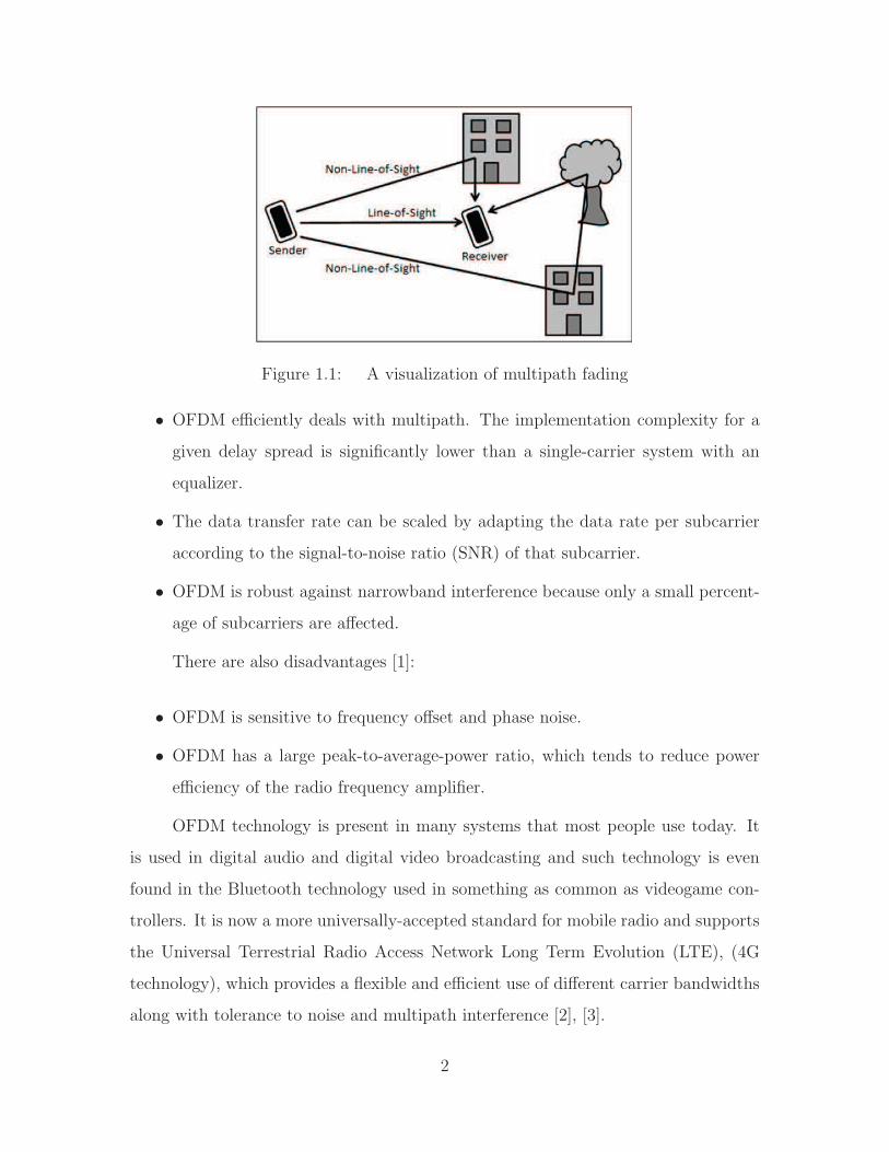
Figure 1.1: A visualization of multipath fading
• OFDM efficiently deals with multipath. The implementation complexity for a
given delay spread is significantly lower than a single-carrier system with an
equalizer.
• The data transfer rate can be scaled by adapting the data rate per subcarrier
according to the signal-to-noise ratio (SNR) of that subcarrier.
• OFDM is robust against narrowband interference because only a small percent-
age of subcarriers are affected.
There are also disadvantages [1]:
• OFDM is sensitive to frequency offset and phase noise.
• OFDM has a large peak-to-average-power ratio, which tends to reduce power
efficiency of the radio frequency amplifier.
OFDM technology is present in many systems that most people use today. It
is used in digital audio and digital video broadcasting and such technology is even
found in the Bluetooth technology used in something as common as videogame con-
trollers. It is now a more universally-accepted standard for mobile radio and supports
the Universal Terrestrial Radio Access Network Long Term Evolution (LTE), (4G
technology), which provides a flexible and efficient use of different carrier bandwidths
along with tolerance to noise and multipath interference [2], [3].
2
1.2 Motivation
Gaining a better understanding of OFDM technology is the focus of many inter-
ests, including manufacturing, communications, and the government agencies. Veri-
zon Wireless talks about how 4G LTE technology is 10 times faster than 3G technol-
ogy and reduces delay and buffering. This technology is backed by the foundation of
OFDM technology and is now an integral part of many people’s lives [4]. The U.S. Air
Force seeks full spectrum dominance over any and all computers. The Broad Agency
Announcement from Air Force Research Laboratory has announced their desire to
support various scientific studies and experiments to better their knowledge of the
broad range of capabilities required in support of dominant cyber offensive engage-
ment and supporting technology. One of their objectives includes the capability to
provide techniques and technologies to be able to affect computer information systems
through deceive, deny, disrupt, degrade, and destroy (D5) effects [5]. The D5 describe
the broad focus behind signal jamming technologies.
This thesis presents the investigation of jamming simulated OFDM signals.
There are many methods of jamming. Some of these include:
• Noise jamming: this technique directs a noise signal to fill the entire band that
the sender is using in order to interfere with the transmission.
• Sense jamming: this technique “senses” when the sender’s signal is in a specific
channel, then fills only the channel in use with noise.
• Deceptive jamming: this technique records the signals between the sender and
receiver in order to send out similar signals to “confuse” the receiver.
• Selective jamming: this technique detects a specific transmission in the pool of
signals and jams only that transmission.
This research, however, investigates two different jamming methods in the time-
domain, noise jamming and a variation of noise jamming, CP-jamming. CP-jamming
sends noise signals to only the cyclic prefix of each symbol in a given signal with
3
the desire of skewing the symbol-time delay correction at the receiver. These two
techniques are tested in three different channel conditions and the effectiveness of
each technique is compared by using bit error rate (BER) plots.
OFDM systems have become a basis for wireless communications as well as
other applications and research has focused on the analysis and implementation of
OFDM to better fortify existing systems. With so many systems integrating OFDM
concepts, it is only natural to try to find a way to most effectively interfere or break
those systems. This research is a foundation for jamming OFDM systems and it starts
by researching the effects of two methods of jamming a simple OFDM signal.
1.3 Goals
This research takes a better look at the effects of jamming the CP of an OFDM
signal against the traditional noise jamming technique, Fig. 1.2. The comparison
is made in multiple channel conditions to gain a better insight to which technique
works best in varying environments. The theory behind jamming the CP is simple.
Since the CP is used as a means to correct the symbol-time delay and the carrier
frequency offset of the signal by correlating the repeated parts of a symbol, using
a more concentrated interfering signal in just the CP will throw off the correlation
therefore disrupting the received signal. BER plots are used to compare the jamming
techniques. The comparison shows whether or not estimating where all the CPs are
located in the given signal and then jamming that part of the signal is more effective
than sending a noise signal that disperses its interfering signal power across the entire
signal. More detail is provided in Ch. III. The results are conclusive but are based
on the assumptions and simulations of this research.
1.4 Assumptions
For this research, the following assumptions are made:
4
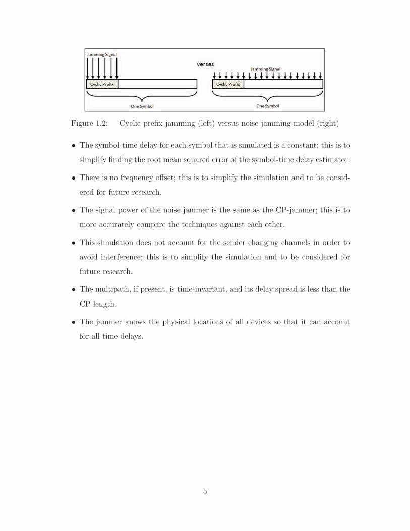
Figure 1.2: Cyclic prefix jamming (left) versus noise jamming model (right)
• The symbol-time delay for each symbol that is simulated is a constant; this is to
simplify finding the root mean squared error of the symbol-time delay estimator.
• There is no frequency offset; this is to simplify the simulation and to be consid-
ered for future research.
• The signal power of the noise jammer is the same as the CP-jammer; this is to
more accurately compare the techniques against each other.
• This simulation does not account for the sender changing channels in order to
avoid interference; this is to simplify the simulation and to be considered for
future research.
• The multipath, if present, is time-invariant, and its delay spread is less than the
CP length.
• The jammer knows the physical locations of all devices so that it can account
for all time delays.
5
II. Background
This chapter provides the background for the topics involved in this research. First,
there is an overview of general information on jamming and how OFDM and LTE
systems cope with interference.
2.1 Jamming Background
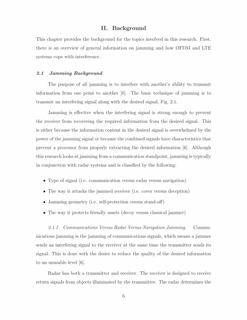
The purpose of all jamming is to interfere with another’s ability to transmit
information from one point to another [6]. The basic technique of jamming is to
transmit an interfering signal along with the desired signal, Fig. 2.1.
Jamming is effective when the interfering signal is strong enough to prevent
the receiver from recovering the required information from the desired signal. This
is either because the information content in the desired signal is overwhelmed by the
power of the jamming signal or because the combined signals have characteristics that
prevent a processor from properly extracting the desired information [6]. Although
this research looks at jamming from a communication standpoint, jamming is typically
in conjunction with radar systems and is classified by the following:
• Type of signal (i.e. communication versus radar versus navigation)
• The way it attacks the jammed receiver (i.e. cover versus deception)
• Jamming geometry (i.e. self-protection versus stand-off)
• The way it protects friendly assets (decoy versus classical jammer)
2.1.1 Communications Versus Radar Versus Navigation Jamming. Commu-
nications jamming is the jamming of communications signals, which means a jammer
sends an interfering signal to the receiver at the same time the transmitter sends its
signal. This is done with the desire to reduce the quality of the desired information
to an unusable level [6].
Radar has both a transmitter and receiver. The receiver is designed to receive
return signals from objects illuminated by the transmitter. The radar determines the
6
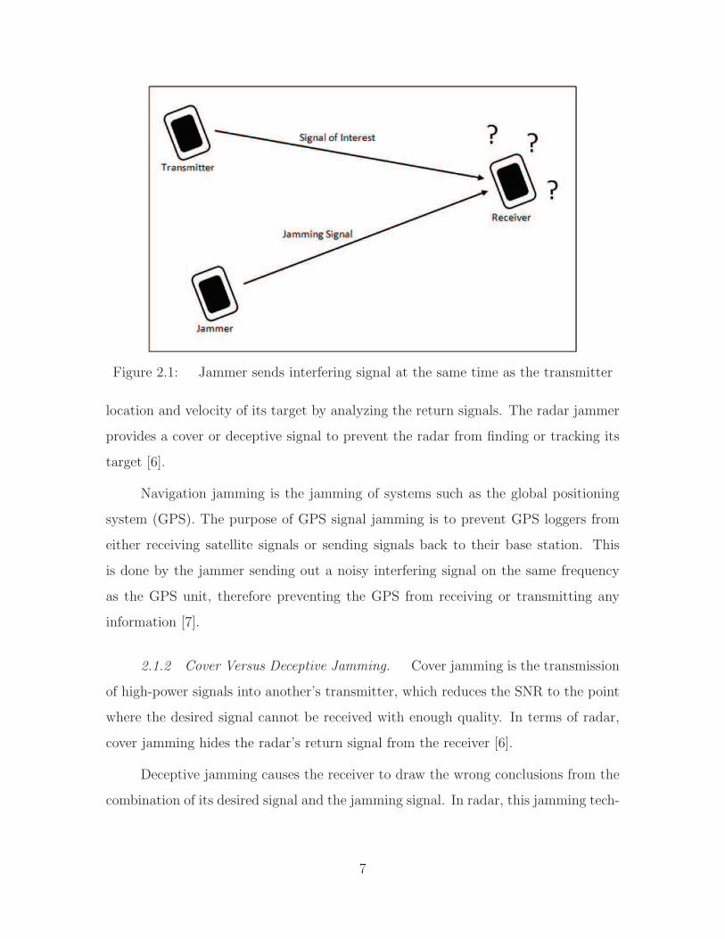
Figure 2.1: Jammer sends interfering signal at the same time as the transmitter
location and velocity of its target by analyzing the return signals. The radar jammer
provides a cover or deceptive signal to prevent the radar from finding or tracking its
target [6].
Navigation jamming is the jamming of systems such as the global positioning
system (GPS). The purpose of GPS signal jamming is to prevent GPS loggers from
either receiving satellite signals or sending signals back to their base station. This
is done by the jammer sending out a noisy interfering signal on the same frequency
as the GPS unit, therefore preventing the GPS from receiving or transmitting any
information [7].
2.1.2 Cover Versus Deceptive Jamming. Cover jamming is the transmission
of high-power signals into another’s transmitter, which reduces the SNR to the point
where the desired signal cannot be received with enough quality. In terms of radar,
cover jamming hides the radar’s return signal from the receiver [6].
Deceptive jamming causes the receiver to draw the wrong conclusions from the
combination of its desired signal and the jamming signal. In radar, this jamming tech-
7
nique gets an apparently valid signal and is tricked into tracking a non-existent/false
target [6].
2.1.3 Self-Protection Versus Stand-Off Jamming. Self-protection jamming
is when the platform being detected or tracked transmits its own jamming signals.
Stand-off jamming is when a jammer on one platform transmits jamming signals to
protect another platform [6].
2.1.4 Decoys Versus Classical Jamming. A decoy is a different kind of
jammer designed to look like a protected platform rather than the protected platform
itself. The difference between decoys and classical jammers is that a decoy does not
interfere with the radars tracking it. Instead, it seeks to attract the attention of those
radars, transferring the focus from the actual target [6].
This research specifically looks at communication jamming and is a basis for
future work in cognitive communications jamming.
2.2 OFDM on Interference
OFDM and LTE systems are designed in a way to efficiently have successful
communication transmissions and to be able to cope with interference, intentional or
not.
As described in Ch. I, OFDM transmits signals using a large number of closely
spaced subcarriers that are modulated at a low data rate. By making the signals
orthogonal to each other, there is no mutual interference. The data transmitted is
split across all the subcarriers and because only some of the subcarriers are lost due
to multipath effects, error correcting techniques can reconstruct the data. Addition-
ally, inserting a cyclic prefix, a copy of the last part of each symbol, to the front
of each symbol helps overcome inter-symbol interference. Its length is selected to be
larger than the maximum anticipated excess delay of the multipath propagation chan-
nel. Due to the cyclic prefix, the transmitted signal is periodic and the effect of the
8
time-dispersive multipath channel becomes equivalent to a cyclic convolution. The
properties of the cyclic convolution allow the subcarriers to remain orthogonal [1].
A detailed model of OFDM is given in Ch. III. The basic concepts of OFDM are a
foundation for LTE.
2.3 LTE on Interference
One key element of LTE is the use of OFDM as the signal bearer. One of the
main reasons for using OFDM as a modulation format within LTE is its resilience to
multipath delay spread, which can account for several microseconds. Moreover, the in-
sertion of a CP adds to the resilience of the system and helps overcome inter-symbol
interference [8], [9]. Both multipath delay spread and user equipment power con-
sumption are important factors in the LTE design, thus LTE implements orthogonal
frequency division multiple access (OFDMA) for downlink transmission and single-
carrier frequency division multiple access (SC-FDMA) for uplink transmission [8].
The difference between OFDM and OFDMA is that OFDMA is a multi-user
OFDM, which allows multiple access on the same channel. This is done by distribut-
ing the subcarriers among users so all users can transmit and receive at the same
time. Further, subchannels are matched to each user to lessen fading and interference
based on the location and propagation characteristics of each user, providing better
transmission performance [10].
OFDMA has a high peak-to-average ratio, which is not a problem for a base
station in the LTE downlink, but the high power consumption of OFDMA is not
acceptable for mobile phones, where battery life is limited. SC-FDMA is a different
access technique used in the LTE uplink. It is a single-carrier transmission scheme
opposed to OFDMA, which is a multi-carrier transmission scheme. The LTE concept
combines the low peak-to-average ratio offered by single-carrier systems with the mul-
tipath interference resilience and flexible subcarrier frequency allocation that OFDM
provides [8].
9
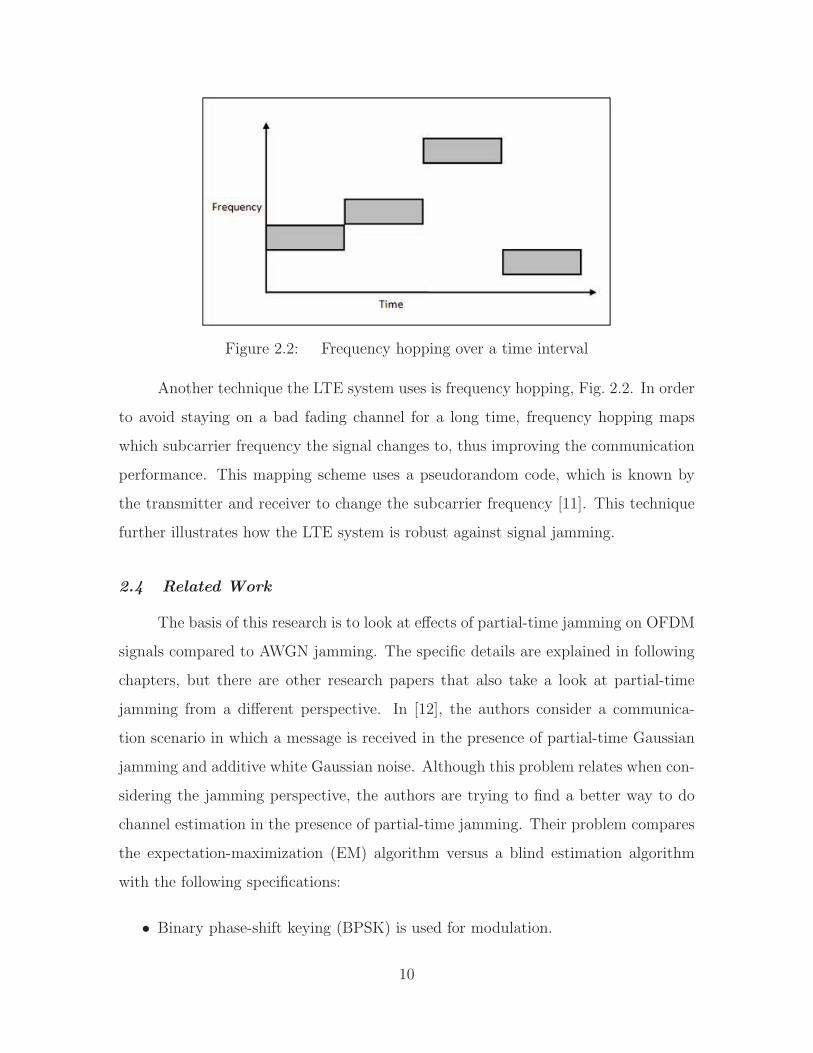
Figure 2.2: Frequency hopping over a time interval
Another technique the LTE system uses is frequency hopping, Fig. 2.2. In order
to avoid staying on a bad fading channel for a long time, frequency hopping maps
which subcarrier frequency the signal changes to, thus improving the communication
performance. This mapping scheme uses a pseudorandom code, which is known by
the transmitter and receiver to change the subcarrier frequency [11]. This technique
further illustrates how the LTE system is robust against signal jamming.
2.4 Related Work
The basis of this research is to look at effects of partial-time jamming on OFDM
signals compared to AWGN jamming. The specific details are explained in following
chapters, but there are other research papers that also take a look at partial-time
jamming from a different perspective. In [12], the authors consider a communica-
tion scenario in which a message is received in the presence of partial-time Gaussian
jamming and additive white Gaussian noise. Although this problem relates when con-
sidering the jamming perspective, the authors are trying to find a better way to do
channel estimation in the presence of partial-time jamming. Their problem compares
the expectation-maximization (EM) algorithm versus a blind estimation algorithm
with the following specifications:
• Binary phase-shift keying (BPSK) is used for modulation.
10
• The system is considered in a quasi-static channel, in which the amplitude and
phase are constant over each packet transmission.
• The jammer is modeled using a two state Markov model. (When the jammer is
in state 0, it does not transmit the jamming signal; when the jammer is in state
1, the jammer does transmit the jamming signal.)
• The receiver does not know the amplitude and phase of the incoming signal.
• The receiver does not know which symbols are jammed or the statistics of the
jammer.
• The receiver must estimate the parameters of the channel and the jamming to
achieve good performance.
In [13], the authors propose new collaborative reception techniques for use in the
presence of a partial-time Gaussian jammer. Under their proposed techniques, a group
of radios acts as a distributed antenna array by exchanging information that is used
to perform jamming mitigation. Their jamming mitigation techniques offer a tradeoff
between performance and complexity [13]. With modifications to the intent of the
research, these two topics provide a foundation for comparing jamming techniques.
11
III. Methodology
This chapter introduces the features of the OFDM signal as well as the mathematical
breakdown of the maximum likelihood symbol-time delay estimator. One of the prob-
lems in the design of OFDM receivers is the unknown symbol arrival time. Sensitivity
to a time offset is higher in multicarrier systems than in single-carrier systems, which
is why a ML estimator for the symbol-time delay is used [14].
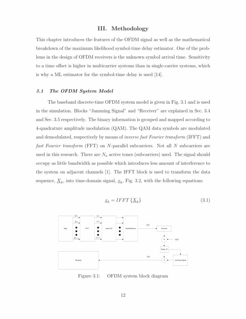
3.1 The OFDM System Model
The baseband discrete-time OFDM system model is given in Fig. 3.1 and is used
in the simulation. Blocks “Jamming Signal” and “Receiver” are explained in Sec. 3.4
and Sec. 3.5 respectively. The binary information is grouped and mapped according to
4-quadrature amplitude modulation (QAM). The QAM data symbols are modulated
and demodulated, respectively by means of inverse fast Fourier transform (IFFT) and
fast Fourier transform (FFT) on N -parallel subcarriers. Not all N subcarriers are
used in this research. There are Na active tones (subcarriers) used. The signal should
occupy as little bandwidth as possible which introduces less amount of interference to
the system on adjacent channels [1]. The IFFT block is used to transform the data
sequence, Xk, into time-domain signal, xk, Fig. 3.2, with the following equations:
xk = IFFT {Xk} (3.1)
Receiver
Channel
Delay, Ɵ
n(t)
s(t)
+
+
r(t)
Map IFFT Insert CP Parallel/Series
Jamming Signal
X0,k
X1,k
XN-1,k
x0,k
x1,k
xN-1,k
Figure 3.1: OFDM system block diagram
12
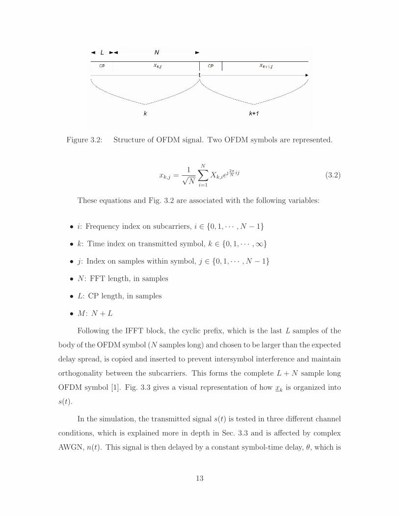
Figure 3.2: Structure of OFDM signal. Two OFDM symbols are represented.
xk,j =1√N
N∑
i=1
Xk,ie 2πN
ij (3.2)
These equations and Fig. 3.2 are associated with the following variables:
• i: Frequency index on subcarriers, i ∈ {0, 1, · · · , N − 1}
• k: Time index on transmitted symbol, k ∈ {0, 1, · · · ,∞}
• j: Index on samples within symbol, j ∈ {0, 1, · · · , N − 1}
• N : FFT length, in samples
• L: CP length, in samples
• M : N + L
Following the IFFT block, the cyclic prefix, which is the last L samples of the
body of the OFDM symbol (N samples long) and chosen to be larger than the expected
delay spread, is copied and inserted to prevent intersymbol interference and maintain
orthogonality between the subcarriers. This forms the complete L + N sample long
OFDM symbol [1]. Fig. 3.3 gives a visual representation of how xk is organized into
s(t).
In the simulation, the transmitted signal s(t) is tested in three different channel
conditions, which is explained more in depth in Sec. 3.3 and is affected by complex
AWGN, n(t). This signal is then delayed by a constant symbol-time delay, θ, which is
13
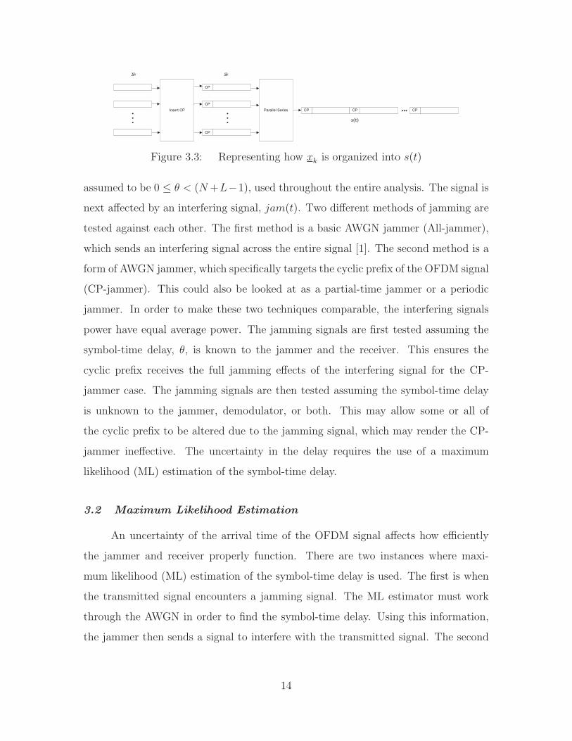
xk
CP
CP
CP
Insert CP Parallel Series CP CP CP
sk
s(t)•
•
•
•
•
•
•••
Figure 3.3: Representing how xk is organized into s(t)
assumed to be 0 ≤ θ < (N+L−1), used throughout the entire analysis. The signal is
next affected by an interfering signal, jam(t). Two different methods of jamming are
tested against each other. The first method is a basic AWGN jammer (All-jammer),
which sends an interfering signal across the entire signal [1]. The second method is a
form of AWGN jammer, which specifically targets the cyclic prefix of the OFDM signal
(CP-jammer). This could also be looked at as a partial-time jammer or a periodic
jammer. In order to make these two techniques comparable, the interfering signals
power have equal average power. The jamming signals are first tested assuming the
symbol-time delay, θ, is known to the jammer and the receiver. This ensures the
cyclic prefix receives the full jamming effects of the interfering signal for the CP-
jammer case. The jamming signals are then tested assuming the symbol-time delay
is unknown to the jammer, demodulator, or both. This may allow some or all of
the cyclic prefix to be altered due to the jamming signal, which may render the CP-
jammer ineffective. The uncertainty in the delay requires the use of a maximum
likelihood (ML) estimation of the symbol-time delay.
3.2 Maximum Likelihood Estimation
An uncertainty of the arrival time of the OFDM signal affects how efficiently
the jammer and receiver properly function. There are two instances where maxi-
mum likelihood (ML) estimation of the symbol-time delay is used. The first is when
the transmitted signal encounters a jamming signal. The ML estimator must work
through the AWGN in order to find the symbol-time delay. Using this information,
the jammer then sends a signal to interfere with the transmitted signal. The second
14
time the ML estimator is used is after the signal is received. The ML estimator must
work through the AWGN and possibly the jamming signal in order to correct the
symbol-time delay for demodulating. The following equation represents the symbol-
time delay as well as AWGN and the jamming signal at the receiver.
r(t) = s(t− θ) + n(t) + jam(t) (3.3)
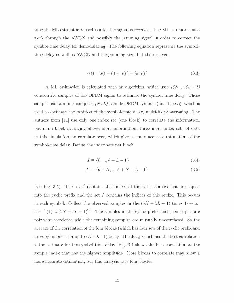
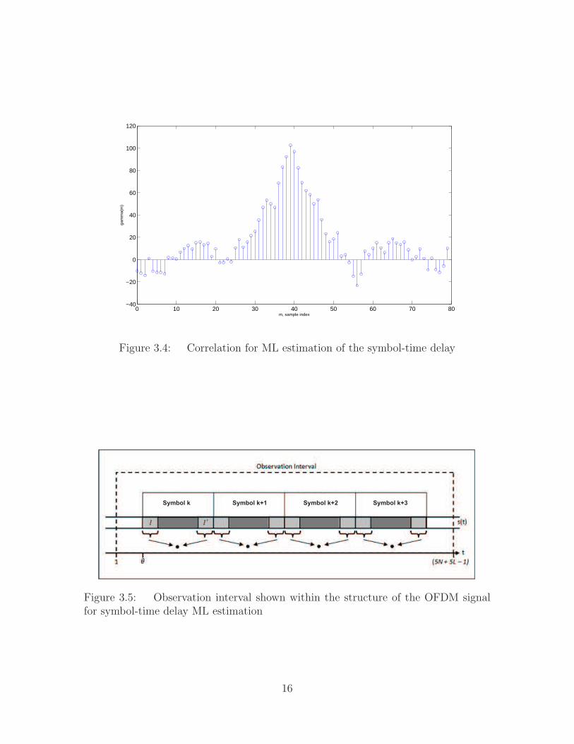
A ML estimation is calculated with an algorithm, which uses (5N + 5L - 1)
consecutive samples of the OFDM signal to estimate the symbol-time delay. These
samples contain four complete (N+L)-sample OFDM symbols (four blocks), which is
used to estimate the position of the symbol-time delay, multi-block averaging. The
authors from [14] use only one index set (one block) to correlate the information,
but multi-block averaging allows more information, three more index sets of data
in this simulation, to correlate over, which gives a more accurate estimation of the
symbol-time delay. Define the index sets per block
I ≡ {θ, ..., θ + L− 1} (3.4)
I′ ≡ {θ +N, ..., θ +N + L− 1} (3.5)
(see Fig. 3.5). The set I′
contains the indices of the data samples that are copied
into the cyclic prefix and the set I contains the indices of this prefix. This occurs
in each symbol. Collect the observed samples in the (5N + 5L − 1) times 1-vector
r ≡ [r(1)...r(5N + 5L − 1)]T . The samples in the cyclic prefix and their copies are
pair-wise correlated while the remaining samples are mutually uncorrelated. So the
average of the correlation of the four blocks (which has four sets of the cyclic prefix and
its copy) is taken for up to (N+L−1) delay. The delay which has the best correlation
is the estimate for the symbol-time delay. Fig. 3.4 shows the best correlation as the
sample index that has the highest amplitude. More blocks to correlate may allow a
more accurate estimation, but this analysis uses four blocks.
15
0 10 20 30 40 50 60 70 80−40
−20
0
20
40
60
80
100
120ga
mm
a(m
)
m, sample index
Figure 3.4: Correlation for ML estimation of the symbol-time delay
Symbol k Symbol k+1 Symbol k+2 Symbol k+3
Figure 3.5: Observation interval shown within the structure of the OFDM signalfor symbol-time delay ML estimation
16
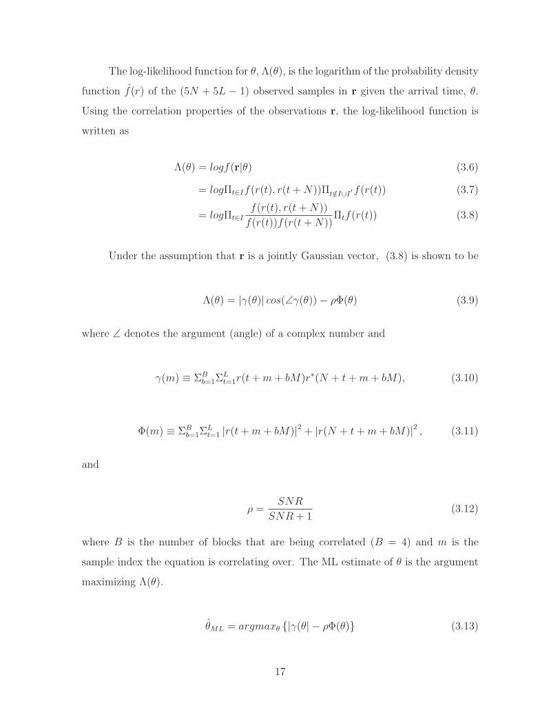
The log-likelihood function for θ, Λ(θ), is the logarithm of the probability density
function f(r) of the (5N + 5L − 1) observed samples in r given the arrival time, θ.
Using the correlation properties of the observations r, the log-likelihood function is
written as
Λ(θ) = logf(r|θ) (3.6)
= logΠt∈If(r(t), r(t+N))Πt/∈I∪I′f(r(t)) (3.7)
= logΠt∈If(r(t), r(t+N))
f(r(t))f(r(t+N))Πtf(r(t)) (3.8)
Under the assumption that r is a jointly Gaussian vector, (3.8) is shown to be
Λ(θ) = |γ(θ)| cos(∠γ(θ))− ρΦ(θ) (3.9)
where ∠ denotes the argument (angle) of a complex number and
γ(m) ≡ ΣBb=1Σ
Lt=1r(t+m+ bM)r∗(N + t+m+ bM), (3.10)
Φ(m) ≡ ΣBb=1Σ
Lt=1 |r(t+m+ bM)|2 + |r(N + t+m+ bM)|2 , (3.11)
and
ρ =SNR
SNR + 1(3.12)
where B is the number of blocks that are being correlated (B = 4) and m is the
sample index the equation is correlating over. The ML estimate of θ is the argument
maximizing Λ(θ).
θML = argmaxθ {|γ(θ| − ρΦ(θ)} (3.13)
17
Eqs. (3.6)- (3.13) are from [14] simplified for no carrier frequency offset.
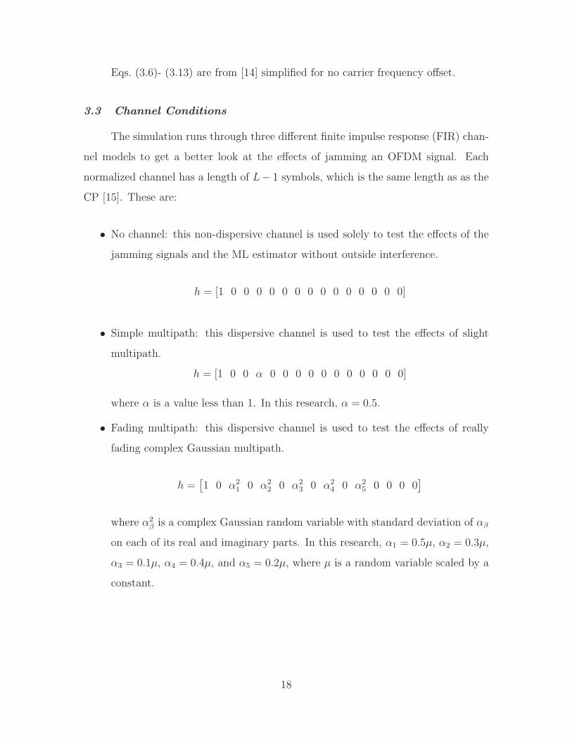
3.3 Channel Conditions
The simulation runs through three different finite impulse response (FIR) chan-
nel models to get a better look at the effects of jamming an OFDM signal. Each
normalized channel has a length of L− 1 symbols, which is the same length as as the
CP [15]. These are:
• No channel: this non-dispersive channel is used solely to test the effects of the
jamming signals and the ML estimator without outside interference.
h = [1 0 0 0 0 0 0 0 0 0 0 0 0 0 0]
• Simple multipath: this dispersive channel is used to test the effects of slight
multipath.
h = [1 0 0 α 0 0 0 0 0 0 0 0 0 0 0]
where α is a value less than 1. In this research, α = 0.5.
• Fading multipath: this dispersive channel is used to test the effects of really
fading complex Gaussian multipath.
h =[
1 0 α21 0 α2
2 0 α23 0 α2
4 0 α25 0 0 0 0
]
where α2β is a complex Gaussian random variable with standard deviation of αβ
on each of its real and imaginary parts. In this research, α1 = 0.5µ, α2 = 0.3µ,
α3 = 0.1µ, α4 = 0.4µ, and α5 = 0.2µ, where µ is a random variable scaled by a
constant.
18
Jamming Signal
ML Est
θ^
jam(t-θ) jam(t)^
s(t-θ)+n(t-θ)
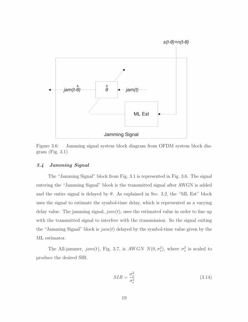
Figure 3.6: Jamming signal system block diagram from OFDM system block dia-gram (Fig. 3.1)
3.4 Jamming Signal
The “Jamming Signal” block from Fig. 3.1 is represented in Fig. 3.6. The signal
entering the “Jamming Signal” block is the transmitted signal after AWGN is added
and the entire signal is delayed by θ. As explained in Sec. 3.2, the “ML Est” block
uses the signal to estimate the symbol-time delay, which is represented as a varying
delay value. The jamming signal, jam(t), uses the estimated value in order to line up
with the transmitted signal to interfere with the transmission. So the signal exiting
the “Jamming Signal” block is jam(t) delayed by the symbol-time value given by the
ML estimator.
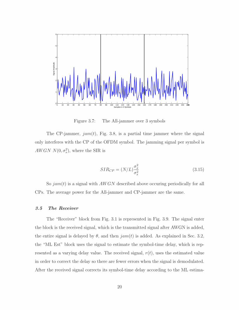
The All-jammer, jam(t), Fig. 3.7, is AWGN N(0, σ2s), where σ2
s is scaled to
produce the desired SIR.
SIR =σ2x
σ2s
(3.14)
19
0 10 20 30 40 50 60 70 80 90 100 110 120 130 140 150 160 170 180 190 200 210 220 230 2402400
1
2
3
4
5
6
Samples in 3 Symbols
Sig
nal A
mpl
itude
Figure 3.7: The All-jammer over 3 symbols
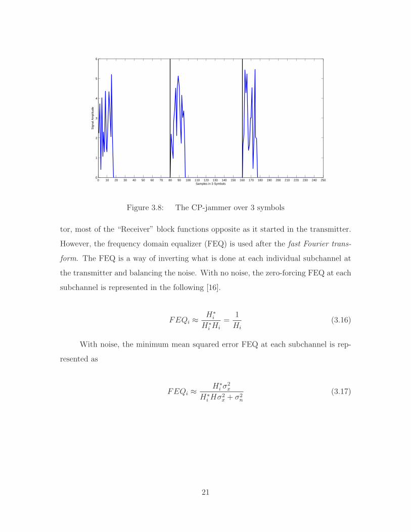
The CP-jammer, jam(t), Fig. 3.8, is a partial time jammer where the signal
only interferes with the CP of the OFDM symbol. The jamming signal per symbol is
AWGN N(0, σ2s), where the SIR is
SIRCP = (N/L)σ2x
σ2s
(3.15)
So jam(t) is a signal with AWGN described above occuring periodically for all
CPs. The average power for the All-jammer and CP-jammer are the same.
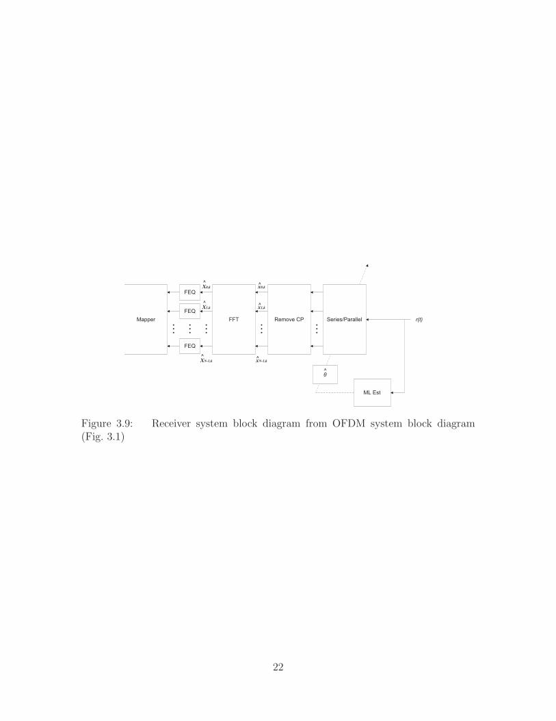
3.5 The Receiver
The “Receiver” block from Fig. 3.1 is represented in Fig. 3.9. The signal enter
the block is the received signal, which is the transmitted signal after AWGN is added,
the entire signal is delayed by θ, and then jam(t) is added. As explained in Sec. 3.2,
the “ML Est” block uses the signal to estimate the symbol-time delay, which is rep-
resented as a varying delay value. The received signal, r(t), uses the estimated value
in order to correct the delay so there are fewer errors when the signal is demodulated.
After the received signal corrects its symbol-time delay according to the ML estima-
20
0 10 20 30 40 50 60 70 80 90 100 110 120 130 140 150 160 170 180 190 200 210 220 230 240 2500
1
2
3
4
5
6
Samples in 3 Symbols
Sig
nal A
mpl
itude
Figure 3.8: The CP-jammer over 3 symbols
tor, most of the “Receiver” block functions opposite as it started in the transmitter.
However, the frequency domain equalizer (FEQ) is used after the fast Fourier trans-
form. The FEQ is a way of inverting what is done at each individual subchannel at
the transmitter and balancing the noise. With no noise, the zero-forcing FEQ at each
subchannel is represented in the following [16].
FEQi ≈H∗
i
H∗i Hi
=1
Hi
(3.16)
With noise, the minimum mean squared error FEQ at each subchannel is rep-
resented as
FEQi ≈H∗
i σ2x
H∗i Hσ2
x + σ2n
(3.17)
21
Mapper FFT Remove CP
FEQ
FEQ
FEQ
Series/Parallel
ML Est
θ^
r(t)•••
•••
•••
•••
•••
X0,k
X1,k
XN-1,k
^
^
^xN-1,k
x1,k
x0,k^
^
^
Figure 3.9: Receiver system block diagram from OFDM system block diagram(Fig. 3.1)
22
IV. Results
This chapter goes over the specifications of the simulations as well as the results and
comparison of the simulations. The framework for the simulation code was adapted
from the Matlab code used in [17], and an older version available at [18].
4.1 Simulations
An OFDM system with 64 subcarriers is simulated to evaluate the effectiveness
of the All-jammer verses the CP-jammer. The simulation is run in three different
channel conditions and with or without the use of the ML estimator at the jammer
and receiver. In each simulation, 15 000 symbols are used, 100 symbols per signal
(Nsym) with 150 (P ) signal trials per simulation. Each symbol has 80 samples, 52× 2
bits of QAM data. There are 52 active tones (Na). The performance of each of the
jamming signals is evaluated against each other by means of a bit error rate (BER)
plot. The performance of the ML estimator, used in specific cases, is evaluated by
means of a root mean squared error (RMSE) plot. Each simulation compares the
case where there is no jamming, All-jamming, and CP-jamming at different signal-
to-interference ratios (SIR). The SIR values evaluated are 0, 10, and 20 dB. Each
case is also evaluated at signal-to-noise ratios (SNR) between 0 and 20 dB. BERs are
calculated for each trial with
BERp =∆
2Na(Nsym)(4.1)
where ∆ is the total number of bit errors in a signal, Na is the number of active tones,
and Nsym is the number of symbols in each signal. Eq. (4.1) accounts for the two bits
per symbol. The BER of each trial in a given case is calculated. The average of the
trials is represented as BERavg. Error bars are determined for each BER plot and
are calculated using Eq. (4.2). The error for BER is a Bernoulli random variable and
is calculated with the following equations [19].
23
ErrorBar =
√
BERavg · (1−BERavg)
P ·N ·Nsym
(4.2)
In order to gauge the performance of the ML estimator, the RMSE of the
symbol-time delay estimator is averaged over P trials. The following equations are
used:
Errorp = θp − θp (4.3)
RMSE =
√
√
√
√
1
P
P∑
p=1
(Errorp)2 (4.4)
Since var(sum) = sum(var) for independent random variables, the error bars
on the sum of the errors is calculated using Eq. (4.5). The 1√P
is because the 1P
in
the average decreases the variance by P and the standard deviation by√P . The
standard deviation of Errorp is represented as σErrorp . Error bars are determined for
each RMSE plot.
ErrorBarRMSE =1√P
· σErrorp (4.5)
4.2 Results
The results are given with variations in channel conditions, use of the ML estima-
tor at the demodulator, and use of the ML estimator at the jammer. The differences
in each simulation is given in Tab. 4.1.
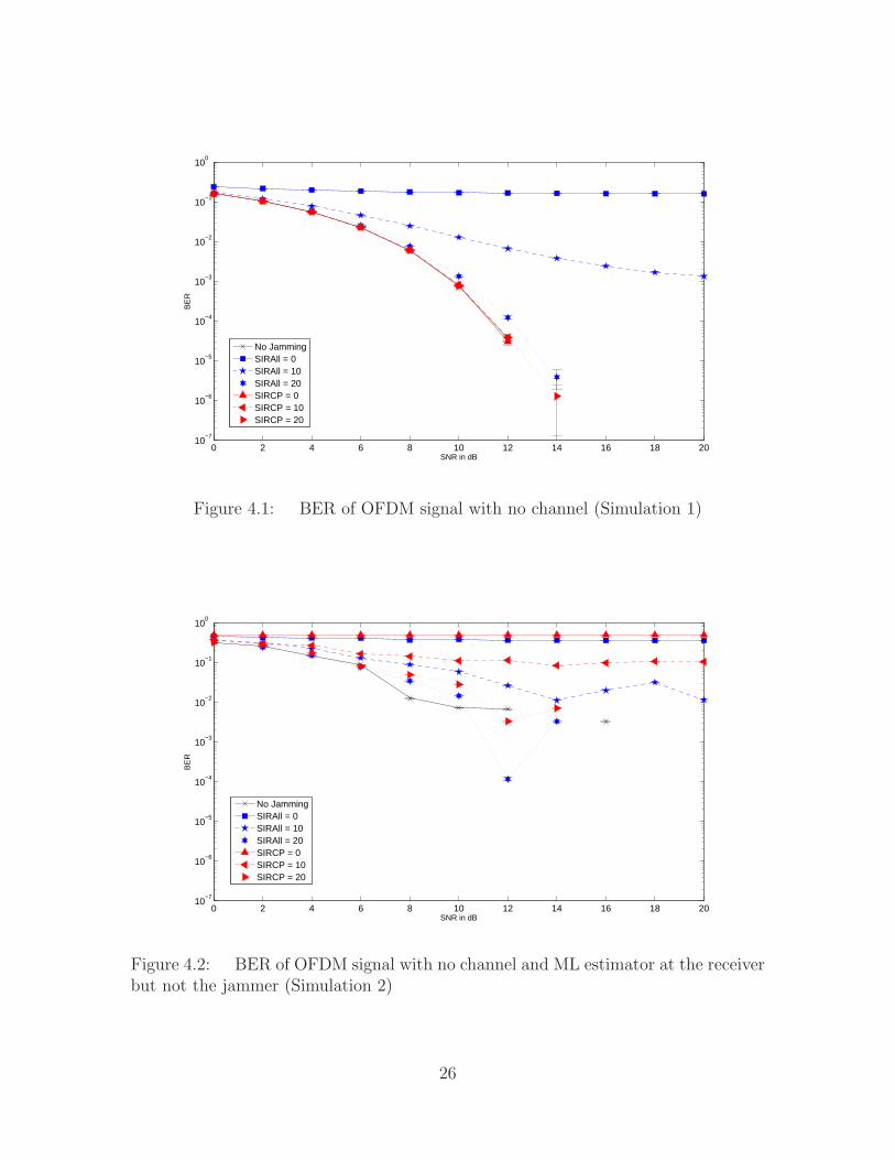
4.2.1 Simulation 1. The first channel case evaluated is having no channel.
The symbol-time delay is known to the jamming signal and the demodulator. Fig. 4.1
shows the All-jammer as a more effective jamming signal compared to the CP-jammer.
The CP-jammer is performing just like the no jamming case. This is expected because
24
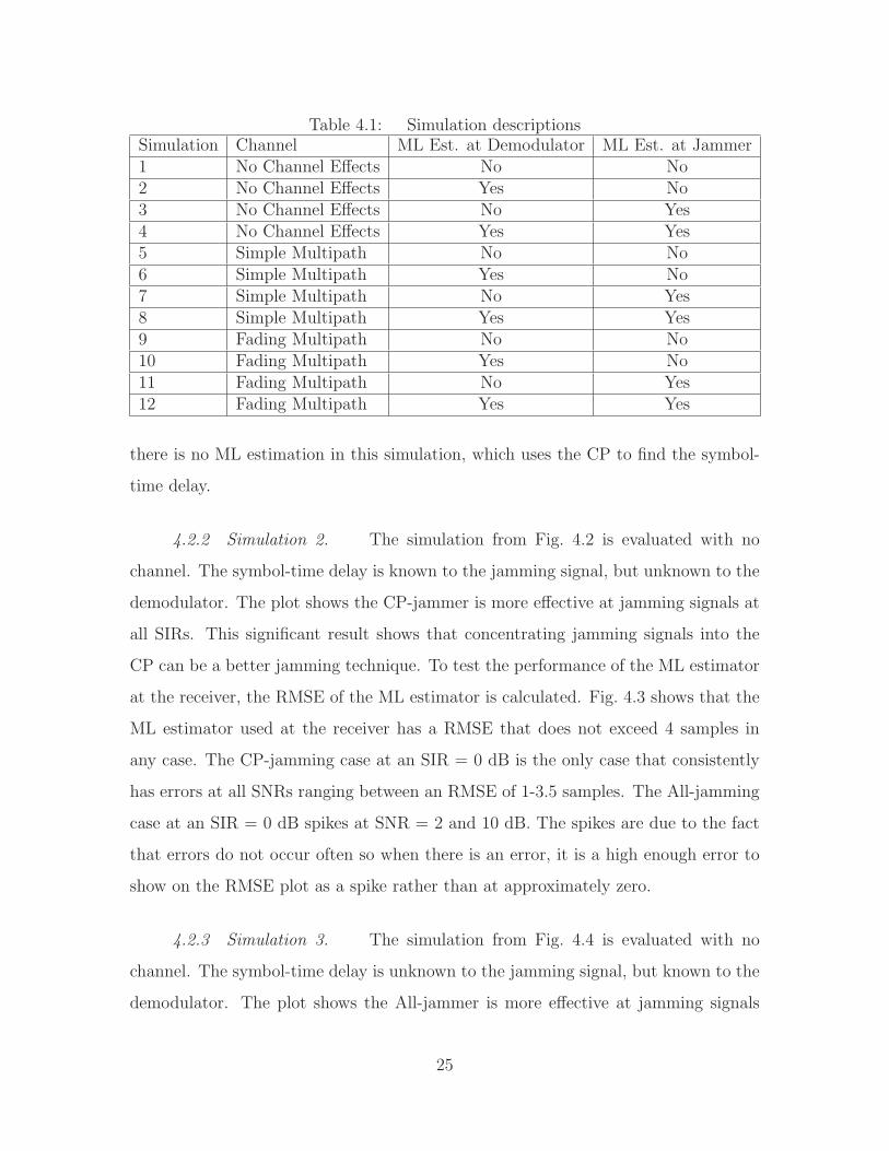
Table 4.1: Simulation descriptionsSimulation Channel ML Est. at Demodulator ML Est. at Jammer1 No Channel Effects No No2 No Channel Effects Yes No3 No Channel Effects No Yes4 No Channel Effects Yes Yes5 Simple Multipath No No6 Simple Multipath Yes No7 Simple Multipath No Yes8 Simple Multipath Yes Yes9 Fading Multipath No No10 Fading Multipath Yes No11 Fading Multipath No Yes12 Fading Multipath Yes Yes
there is no ML estimation in this simulation, which uses the CP to find the symbol-
time delay.
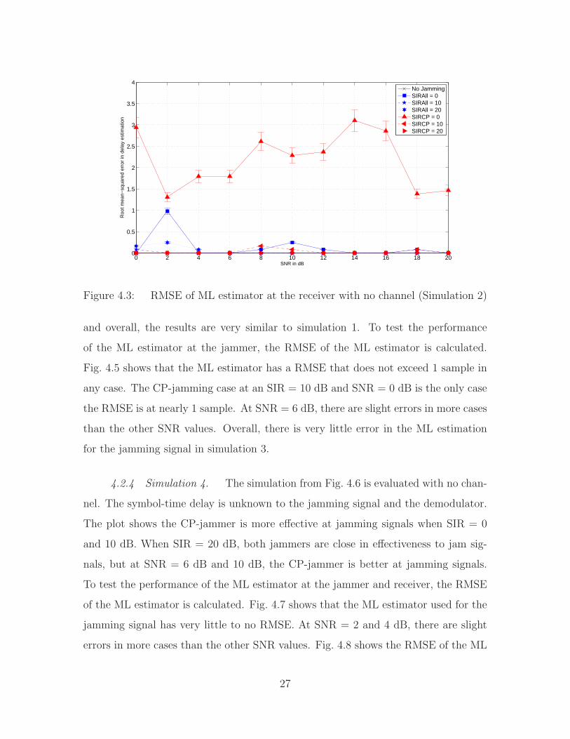
4.2.2 Simulation 2. The simulation from Fig. 4.2 is evaluated with no
channel. The symbol-time delay is known to the jamming signal, but unknown to the
demodulator. The plot shows the CP-jammer is more effective at jamming signals at
all SIRs. This significant result shows that concentrating jamming signals into the
CP can be a better jamming technique. To test the performance of the ML estimator
at the receiver, the RMSE of the ML estimator is calculated. Fig. 4.3 shows that the
ML estimator used at the receiver has a RMSE that does not exceed 4 samples in
any case. The CP-jamming case at an SIR = 0 dB is the only case that consistently
has errors at all SNRs ranging between an RMSE of 1-3.5 samples. The All-jamming
case at an SIR = 0 dB spikes at SNR = 2 and 10 dB. The spikes are due to the fact
that errors do not occur often so when there is an error, it is a high enough error to
show on the RMSE plot as a spike rather than at approximately zero.
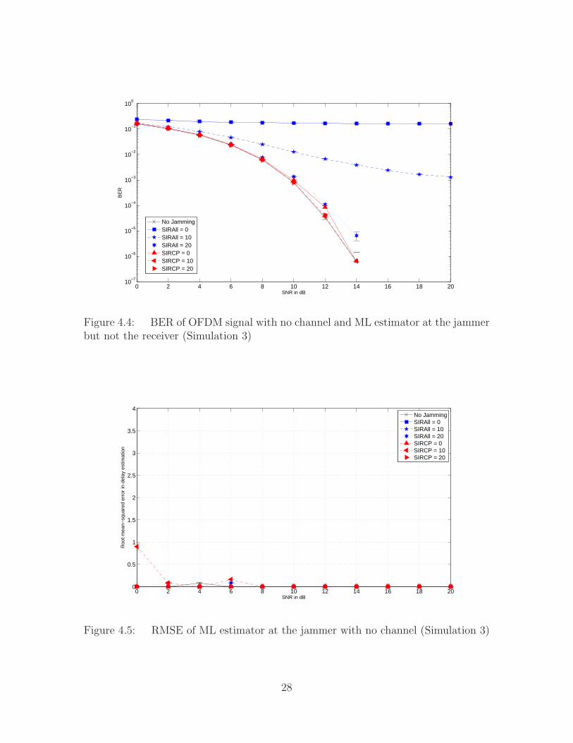
4.2.3 Simulation 3. The simulation from Fig. 4.4 is evaluated with no
channel. The symbol-time delay is unknown to the jamming signal, but known to the
demodulator. The plot shows the All-jammer is more effective at jamming signals
25
0 2 4 6 8 10 12 14 16 18 2010
−7
10−6
10−5
10−4
10−3
10−2
10−1
100
SNR in dB
BE
R
No JammingSIRAll = 0SIRAll = 10SIRAll = 20SIRCP = 0SIRCP = 10SIRCP = 20
Figure 4.1: BER of OFDM signal with no channel (Simulation 1)
0 2 4 6 8 10 12 14 16 18 2010
−7
10−6
10−5
10−4
10−3
10−2
10−1
100
SNR in dB
BE
R
No JammingSIRAll = 0SIRAll = 10SIRAll = 20SIRCP = 0SIRCP = 10SIRCP = 20
Figure 4.2: BER of OFDM signal with no channel and ML estimator at the receiverbut not the jammer (Simulation 2)
26
0 2 4 6 8 10 12 14 16 18 200
0.5
1
1.5
2
2.5
3
3.5
4
SNR in dB
Roo
t mea
n−sq
uare
d er
ror
in d
elay
est
imat
ion
No JammingSIRAll = 0SIRAll = 10SIRAll = 20SIRCP = 0SIRCP = 10SIRCP = 20
Figure 4.3: RMSE of ML estimator at the receiver with no channel (Simulation 2)
and overall, the results are very similar to simulation 1. To test the performance
of the ML estimator at the jammer, the RMSE of the ML estimator is calculated.
Fig. 4.5 shows that the ML estimator has a RMSE that does not exceed 1 sample in
any case. The CP-jamming case at an SIR = 10 dB and SNR = 0 dB is the only case
the RMSE is at nearly 1 sample. At SNR = 6 dB, there are slight errors in more cases
than the other SNR values. Overall, there is very little error in the ML estimation
for the jamming signal in simulation 3.
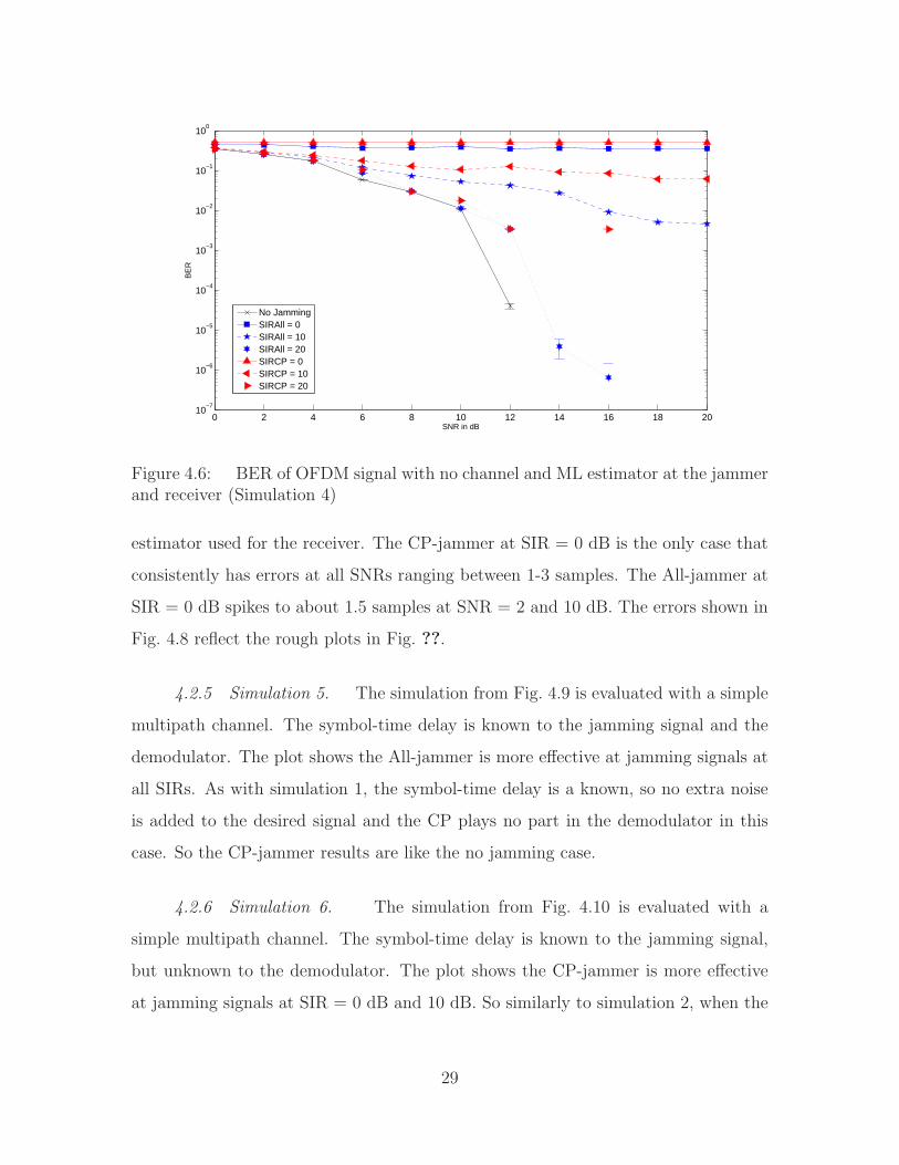
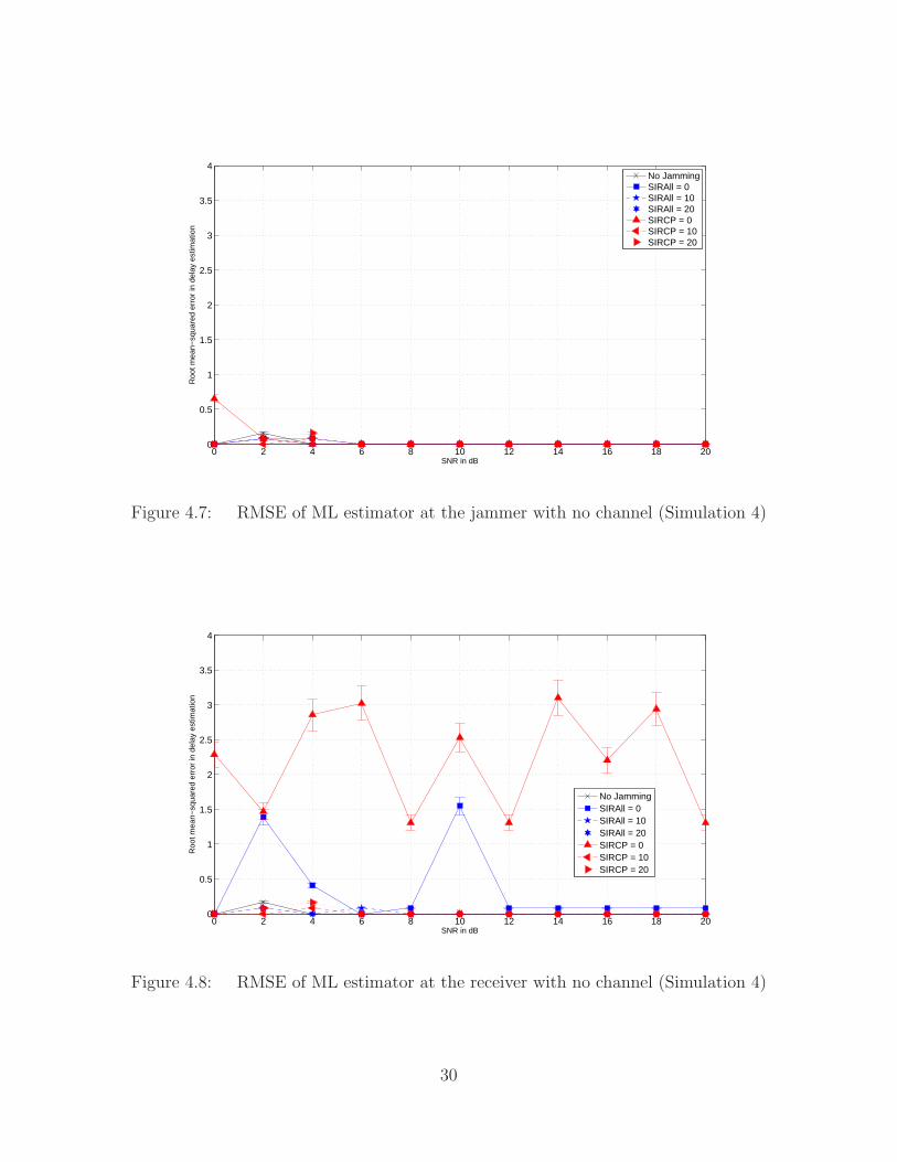
4.2.4 Simulation 4. The simulation from Fig. 4.6 is evaluated with no chan-
nel. The symbol-time delay is unknown to the jamming signal and the demodulator.
The plot shows the CP-jammer is more effective at jamming signals when SIR = 0
and 10 dB. When SIR = 20 dB, both jammers are close in effectiveness to jam sig-
nals, but at SNR = 6 dB and 10 dB, the CP-jammer is better at jamming signals.
To test the performance of the ML estimator at the jammer and receiver, the RMSE
of the ML estimator is calculated. Fig. 4.7 shows that the ML estimator used for the
jamming signal has very little to no RMSE. At SNR = 2 and 4 dB, there are slight
errors in more cases than the other SNR values. Fig. 4.8 shows the RMSE of the ML
27
0 2 4 6 8 10 12 14 16 18 2010
−7
10−6
10−5
10−4
10−3
10−2
10−1
100
SNR in dB
BE
R
No JammingSIRAll = 0SIRAll = 10SIRAll = 20SIRCP = 0SIRCP = 10SIRCP = 20
Figure 4.4: BER of OFDM signal with no channel and ML estimator at the jammerbut not the receiver (Simulation 3)
0 2 4 6 8 10 12 14 16 18 200
0.5
1
1.5
2
2.5
3
3.5
4
SNR in dB
Roo
t mea
n−sq
uare
d er
ror
in d
elay
est
imat
ion
No JammingSIRAll = 0SIRAll = 10SIRAll = 20SIRCP = 0SIRCP = 10SIRCP = 20
Figure 4.5: RMSE of ML estimator at the jammer with no channel (Simulation 3)
28
0 2 4 6 8 10 12 14 16 18 2010
−7
10−6
10−5
10−4
10−3
10−2
10−1
100
SNR in dB
BE
R
No JammingSIRAll = 0SIRAll = 10SIRAll = 20SIRCP = 0SIRCP = 10SIRCP = 20
Figure 4.6: BER of OFDM signal with no channel and ML estimator at the jammerand receiver (Simulation 4)
estimator used for the receiver. The CP-jammer at SIR = 0 dB is the only case that
consistently has errors at all SNRs ranging between 1-3 samples. The All-jammer at
SIR = 0 dB spikes to about 1.5 samples at SNR = 2 and 10 dB. The errors shown in
Fig. 4.8 reflect the rough plots in Fig. ??.
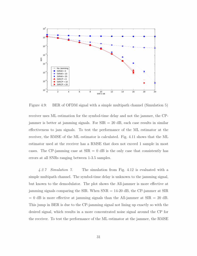
4.2.5 Simulation 5. The simulation from Fig. 4.9 is evaluated with a simple
multipath channel. The symbol-time delay is known to the jamming signal and the
demodulator. The plot shows the All-jammer is more effective at jamming signals at
all SIRs. As with simulation 1, the symbol-time delay is a known, so no extra noise
is added to the desired signal and the CP plays no part in the demodulator in this
case. So the CP-jammer results are like the no jamming case.
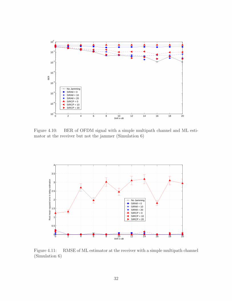
4.2.6 Simulation 6. The simulation from Fig. 4.10 is evaluated with a
simple multipath channel. The symbol-time delay is known to the jamming signal,
but unknown to the demodulator. The plot shows the CP-jammer is more effective
at jamming signals at SIR = 0 dB and 10 dB. So similarly to simulation 2, when the
29
0 2 4 6 8 10 12 14 16 18 200
0.5
1
1.5
2
2.5
3
3.5
4
SNR in dB
Roo
t mea
n−sq
uare
d er
ror
in d
elay
est
imat
ion
No JammingSIRAll = 0SIRAll = 10SIRAll = 20SIRCP = 0SIRCP = 10SIRCP = 20
Figure 4.7: RMSE of ML estimator at the jammer with no channel (Simulation 4)
0 2 4 6 8 10 12 14 16 18 200
0.5
1
1.5
2
2.5
3
3.5
4
SNR in dB
Roo
t mea
n−sq
uare
d er
ror
in d
elay
est
imat
ion
No JammingSIRAll = 0SIRAll = 10SIRAll = 20SIRCP = 0SIRCP = 10SIRCP = 20
Figure 4.8: RMSE of ML estimator at the receiver with no channel (Simulation 4)
30
0 2 4 6 8 10 12 14 16 18 2010
−7
10−6
10−5
10−4
10−3
10−2
10−1
100
SNR in dB
BE
R
No JammingSIRAll = 0SIRAll = 10SIRAll = 20SIRCP = 0SIRCP = 10SIRCP = 20
Figure 4.9: BER of OFDM signal with a simple multipath channel (Simulation 5)
receiver uses ML estimation for the symbol-time delay and not the jammer, the CP-
jammer is better at jamming signals. For SIR = 20 dB, each case results in similar
effectiveness to jam signals. To test the performance of the ML estimator at the
receiver, the RMSE of the ML estimator is calculated. Fig. 4.11 shows that the ML
estimator used at the receiver has a RMSE that does not exceed 1 sample in most
cases. The CP-jamming case at SIR = 0 dB is the only case that consistently has
errors at all SNRs ranging between 1-3.5 samples.
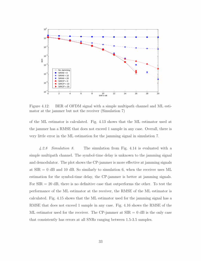
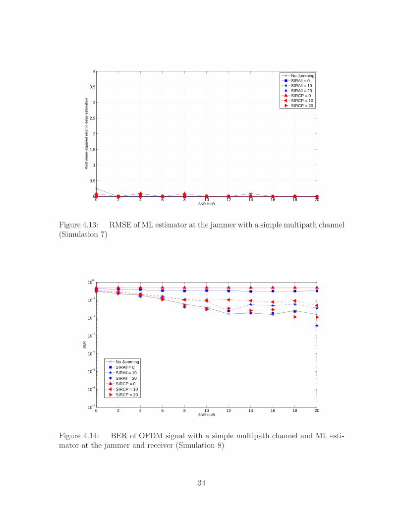
4.2.7 Simulation 7. The simulation from Fig. 4.12 is evaluated with a
simple multipath channel. The symbol-time delay is unknown to the jamming signal,
but known to the demodulator. The plot shows the All-jammer is more effective at
jamming signals comparing the SIR. When SNR = 14-20 dB, the CP-jammer at SIR
= 0 dB is more effective at jamming signals than the All-jammer at SIR = 20 dB.
This jump in BER is due to the CP-jamming signal not lining up exactly so with the
desired signal, which results in a more concentrated noise signal around the CP for
the receiver. To test the performance of the ML estimator at the jammer, the RMSE
31
0 2 4 6 8 10 12 14 16 18 2010
−7
10−6
10−5
10−4
10−3
10−2
10−1
100
SNR in dB
BE
R
No JammingSIRAll = 0SIRAll = 10SIRAll = 20SIRCP = 0SIRCP = 10SIRCP = 20
Figure 4.10: BER of OFDM signal with a simple multipath channel and ML esti-mator at the receiver but not the jammer (Simulation 6)
0 2 4 6 8 10 12 14 16 18 200
0.5
1
1.5
2
2.5
3
3.5
4
SNR in dB
Roo
t mea
n−sq
uare
d er
ror
in d
elay
est
imat
ion
No JammingSIRAll = 0SIRAll = 10SIRAll = 20SIRCP = 0SIRCP = 10SIRCP = 20
Figure 4.11: RMSE of ML estimator at the receiver with a simple multipath channel(Simulation 6)
32
0 2 4 6 8 10 12 14 16 18 2010
−7
10−6
10−5
10−4
10−3
10−2
10−1
100
SNR in dB
BE
R
No JammingSIRAll = 0SIRAll = 10SIRAll = 20SIRCP = 0SIRCP = 10SIRCP = 20
Figure 4.12: BER of OFDM signal with a simple multipath channel and ML esti-mator at the jammer but not the receiver (Simulation 7)
of the ML estimator is calculated. Fig. 4.13 shows that the ML estimator used at
the jammer has a RMSE that does not exceed 1 sample in any case. Overall, there is
very little error in the ML estimation for the jamming signal in simulation 7.
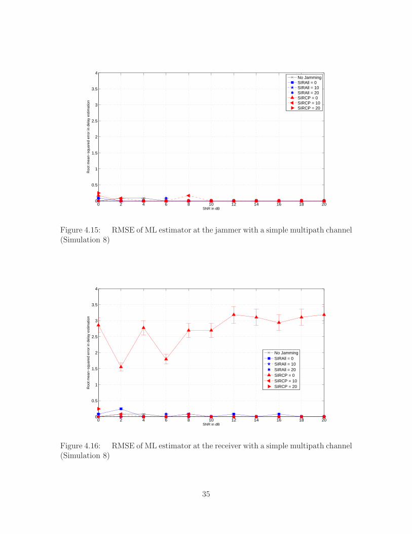
4.2.8 Simulation 8. The simulation from Fig. 4.14 is evaluated with a
simple multipath channel. The symbol-time delay is unknown to the jamming signal
and demodulator. The plot shows the CP-jammer is more effective at jamming signals
at SIR = 0 dB and 10 dB. So similarly to simulation 6, when the receiver uses ML
estimation for the symbol-time delay, the CP-jammer is better at jamming signals.
For SIR = 20 dB, there is no definitive case that outperforms the other. To test the
performance of the ML estimator at the receiver, the RMSE of the ML estimator is
calculated. Fig. 4.15 shows that the ML estimator used for the jamming signal has a
RMSE that does not exceed 1 sample in any case. Fig. 4.16 shows the RMSE of the
ML estimator used for the receiver. The CP-jammer at SIR = 0 dB is the only case
that consistently has errors at all SNRs ranging between 1.5-3.5 samples.
33
0 2 4 6 8 10 12 14 16 18 200
0.5
1
1.5
2
2.5
3
3.5
4
SNR in dB
Roo
t mea
n−sq
uare
d er
ror
in d
elay
est
imat
ion
No JammingSIRAll = 0SIRAll = 10SIRAll = 20SIRCP = 0SIRCP = 10SIRCP = 20
Figure 4.13: RMSE of ML estimator at the jammer with a simple multipath channel(Simulation 7)
0 2 4 6 8 10 12 14 16 18 2010
−7
10−6
10−5
10−4
10−3
10−2
10−1
100
SNR in dB
BE
R
No JammingSIRAll = 0SIRAll = 10SIRAll = 20SIRCP = 0SIRCP = 10SIRCP = 20
Figure 4.14: BER of OFDM signal with a simple multipath channel and ML esti-mator at the jammer and receiver (Simulation 8)
34
0 2 4 6 8 10 12 14 16 18 200
0.5
1
1.5
2
2.5
3
3.5
4
SNR in dB
Roo
t mea
n−sq
uare
d er
ror
in d
elay
est
imat
ion
No JammingSIRAll = 0SIRAll = 10SIRAll = 20SIRCP = 0SIRCP = 10SIRCP = 20
Figure 4.15: RMSE of ML estimator at the jammer with a simple multipath channel(Simulation 8)
0 2 4 6 8 10 12 14 16 18 200
0.5
1
1.5
2
2.5
3
3.5
4
SNR in dB
Roo
t mea
n−sq
uare
d er
ror
in d
elay
est
imat
ion
No JammingSIRAll = 0SIRAll = 10SIRAll = 20SIRCP = 0SIRCP = 10SIRCP = 20
Figure 4.16: RMSE of ML estimator at the receiver with a simple multipath channel(Simulation 8)
35
0 2 4 6 8 10 12 14 16 18 2010
−7
10−6
10−5
10−4
10−3
10−2
10−1
100
SNR in dB
BE
R
No JammingSIRAll = 0SIRAll = 10SIRAll = 20SIRCP = 0SIRCP = 10SIRCP = 20
Figure 4.17: BER of OFDM signal with a fading multipath channel (Simulation 9)
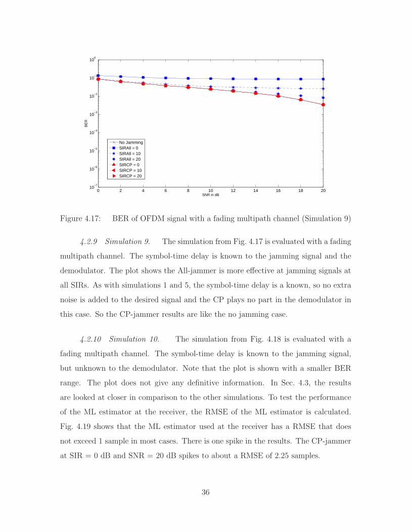
4.2.9 Simulation 9. The simulation from Fig. 4.17 is evaluated with a fading
multipath channel. The symbol-time delay is known to the jamming signal and the
demodulator. The plot shows the All-jammer is more effective at jamming signals at
all SIRs. As with simulations 1 and 5, the symbol-time delay is a known, so no extra
noise is added to the desired signal and the CP plays no part in the demodulator in
this case. So the CP-jammer results are like the no jamming case.
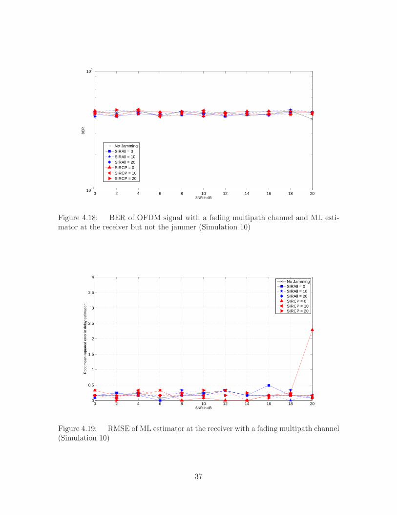
4.2.10 Simulation 10. The simulation from Fig. 4.18 is evaluated with a
fading multipath channel. The symbol-time delay is known to the jamming signal,
but unknown to the demodulator. Note that the plot is shown with a smaller BER
range. The plot does not give any definitive information. In Sec. 4.3, the results
are looked at closer in comparison to the other simulations. To test the performance
of the ML estimator at the receiver, the RMSE of the ML estimator is calculated.
Fig. 4.19 shows that the ML estimator used at the receiver has a RMSE that does
not exceed 1 sample in most cases. There is one spike in the results. The CP-jammer
at SIR = 0 dB and SNR = 20 dB spikes to about a RMSE of 2.25 samples.
36
0 2 4 6 8 10 12 14 16 18 2010
−1
100
SNR in dB
BE
R
No JammingSIRAll = 0SIRAll = 10SIRAll = 20SIRCP = 0SIRCP = 10SIRCP = 20
Figure 4.18: BER of OFDM signal with a fading multipath channel and ML esti-mator at the receiver but not the jammer (Simulation 10)
0 2 4 6 8 10 12 14 16 18 200
0.5
1
1.5
2
2.5
3
3.5
4
SNR in dB
Roo
t mea
n−sq
uare
d er
ror
in d
elay
est
imat
ion
No JammingSIRAll = 0SIRAll = 10SIRAll = 20SIRCP = 0SIRCP = 10SIRCP = 20
Figure 4.19: RMSE of ML estimator at the receiver with a fading multipath channel(Simulation 10)
37
0 2 4 6 8 10 12 14 16 18 2010
−7
10−6
10−5
10−4
10−3
10−2
10−1
100
SNR in dB
BE
R
No JammingSIRAll = 0SIRAll = 10SIRAll = 20SIRCP = 0SIRCP = 10SIRCP = 20
Figure 4.20: BER of OFDM signal with a fading multipath channel and ML esti-mator at the jammer but not the receiver (Simulation 11)
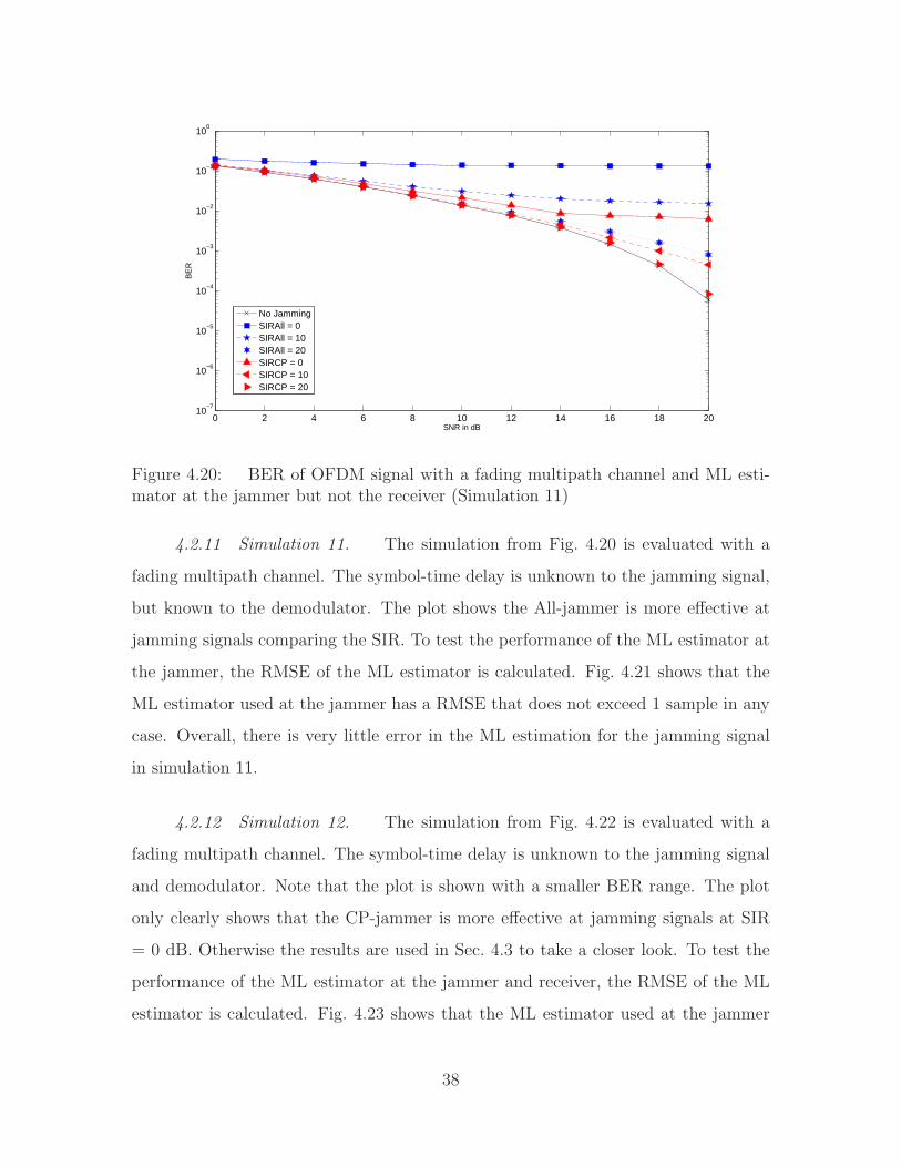
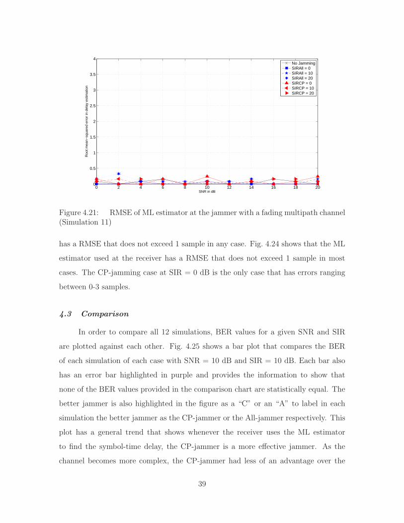
4.2.11 Simulation 11. The simulation from Fig. 4.20 is evaluated with a
fading multipath channel. The symbol-time delay is unknown to the jamming signal,
but known to the demodulator. The plot shows the All-jammer is more effective at
jamming signals comparing the SIR. To test the performance of the ML estimator at
the jammer, the RMSE of the ML estimator is calculated. Fig. 4.21 shows that the
ML estimator used at the jammer has a RMSE that does not exceed 1 sample in any
case. Overall, there is very little error in the ML estimation for the jamming signal
in simulation 11.
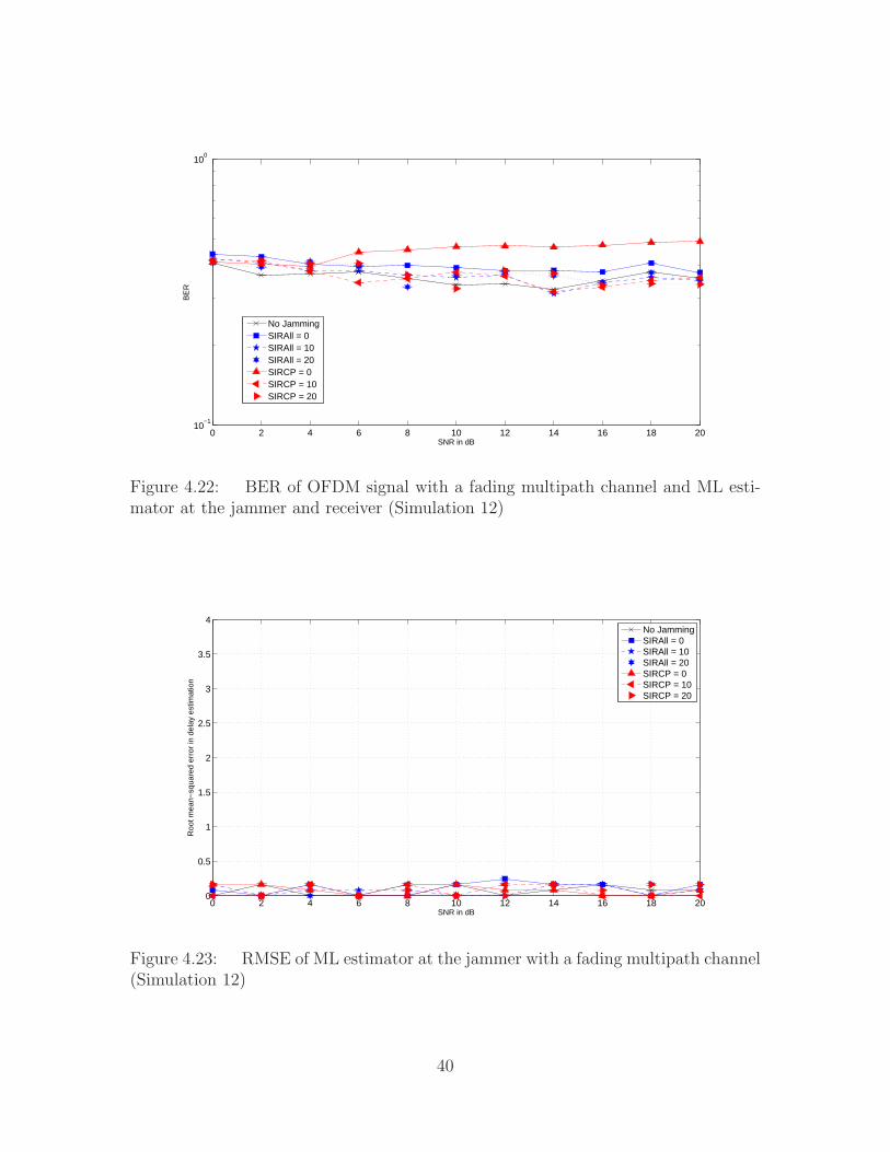
4.2.12 Simulation 12. The simulation from Fig. 4.22 is evaluated with a
fading multipath channel. The symbol-time delay is unknown to the jamming signal
and demodulator. Note that the plot is shown with a smaller BER range. The plot
only clearly shows that the CP-jammer is more effective at jamming signals at SIR
= 0 dB. Otherwise the results are used in Sec. 4.3 to take a closer look. To test the
performance of the ML estimator at the jammer and receiver, the RMSE of the ML
estimator is calculated. Fig. 4.23 shows that the ML estimator used at the jammer
38
0 2 4 6 8 10 12 14 16 18 200
0.5
1
1.5
2
2.5
3
3.5
4
SNR in dB
Roo
t mea
n−sq
uare
d er
ror
in d
elay
est
imat
ion
No JammingSIRAll = 0SIRAll = 10SIRAll = 20SIRCP = 0SIRCP = 10SIRCP = 20
Figure 4.21: RMSE of ML estimator at the jammer with a fading multipath channel(Simulation 11)
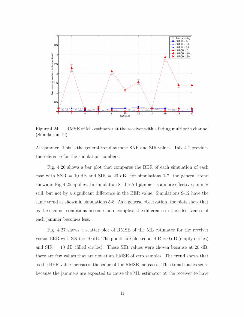
has a RMSE that does not exceed 1 sample in any case. Fig. 4.24 shows that the ML
estimator used at the receiver has a RMSE that does not exceed 1 sample in most
cases. The CP-jamming case at SIR = 0 dB is the only case that has errors ranging
between 0-3 samples.
4.3 Comparison
In order to compare all 12 simulations, BER values for a given SNR and SIR
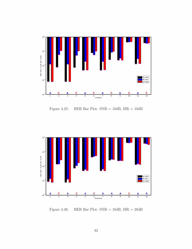
are plotted against each other. Fig. 4.25 shows a bar plot that compares the BER
of each simulation of each case with SNR = 10 dB and SIR = 10 dB. Each bar also
has an error bar highlighted in purple and provides the information to show that
none of the BER values provided in the comparison chart are statistically equal. The
better jammer is also highlighted in the figure as a “C” or an “A” to label in each
simulation the better jammer as the CP-jammer or the All-jammer respectively. This
plot has a general trend that shows whenever the receiver uses the ML estimator
to find the symbol-time delay, the CP-jammer is a more effective jammer. As the
channel becomes more complex, the CP-jammer had less of an advantage over the
39
0 2 4 6 8 10 12 14 16 18 2010
−1
100
SNR in dB
BE
R
No JammingSIRAll = 0SIRAll = 10SIRAll = 20SIRCP = 0SIRCP = 10SIRCP = 20
Figure 4.22: BER of OFDM signal with a fading multipath channel and ML esti-mator at the jammer and receiver (Simulation 12)
0 2 4 6 8 10 12 14 16 18 200
0.5
1
1.5
2
2.5
3
3.5
4
SNR in dB
Roo
t mea
n−sq
uare
d er
ror
in d
elay
est
imat
ion
No JammingSIRAll = 0SIRAll = 10SIRAll = 20SIRCP = 0SIRCP = 10SIRCP = 20
Figure 4.23: RMSE of ML estimator at the jammer with a fading multipath channel(Simulation 12)
40
0 2 4 6 8 10 12 14 16 18 200
0.5
1
1.5
2
2.5
3
3.5
4
SNR in dB
Roo
t mea
n−sq
uare
d er
ror
in d
elay
est
imat
ion
No JammingSIRAll = 0SIRAll = 10SIRAll = 20SIRCP = 0SIRCP = 10SIRCP = 20
Figure 4.24: RMSE of ML estimator at the receiver with a fading multipath channel(Simulation 12)
All-jammer. This is the general trend at most SNR and SIR values. Tab. 4.1 provides
the reference for the simulation numbers.
Fig. 4.26 shows a bar plot that compares the BER of each simulation of each
case with SNR = 10 dB and SIR = 20 dB. For simulations 1-7, the general trend
shown in Fig 4.25 applies. In simulation 8, the All-jammer is a more effective jammer
still, but not by a significant difference in the BER value. Simulations 9-12 have the
same trend as shown in simulations 5-8. As a general observation, the plots show that
as the channel conditions become more complex, the difference in the effectiveness of
each jammer becomes less.
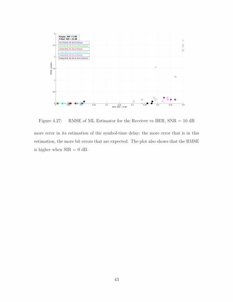
Fig. 4.27 shows a scatter plot of RMSE of the ML estimator for the receiver
versus BER with SNR = 10 dB. The points are plotted at SIR = 0 dB (empty circles)
and SIR = 10 dB (filled circles). These SIR values were chosen because at 20 dB,
there are few values that are not at an RMSE of zero samples. The trend shows that
as the BER value increases, the value of the RMSE increases. This trend makes sense
because the jammers are expected to cause the ML estimator at the receiver to have
41
1 2 3 4 5 6 7 8 9 10 11 1210
−4
10−3
10−2
10−1
100
Simulation
BE
R, S
NR
= 1
0 dB
, SIR
= 1
0 dB
No JamAll JamCP Jam
A A A A AAC C C C C C
Figure 4.25: BER Bar Plot: SNR = 10dB, SIR = 10dB
1 2 3 4 5 6 7 8 9 10 11 1210
−4
10−3
10−2
10−1
100
Simulations
BE
R, S
NR
= 1
0 dB
, SIR
= 2
0 dB
No JamAll JamCP Jam
C C C C AAAAAAA A
Figure 4.26: BER Bar Plot: SNR = 10dB, SIR = 20dB
42
0 0.05 0.1 0.15 0.2 0.25 0.3 0.35 0.4 0.45 0.50
0.5
1
1.5
2
2.5
3
BER, SNR = 10 dB
RM
SE
, sam
ples
Simple Mult, ML Est at Jam & Demod
Fading Mult, ML Est at Jam & Demod
Fading Mult, ML Est at Demod
Simple Mult, ML Est at Demod
No Channel, ML Est at Jam & Demod
No Channel, ML Est at Demod
Empty: SIR = 0 dBFilled: SIR = 10 dB
Figure 4.27: RMSE of ML Estimator for the Receiver vs BER, SNR = 10 dB
more error in its estimation of the symbol-time delay; the more error that is in this
estimation, the more bit errors that are expected. The plot also shows that the RMSE
is higher when SIR = 0 dB.
43

V. Conclusions
This chapter contains concluding comments about the research in this thesis and
recommendations for future work.
5.1 Conclusion
The All-jammer and the CP-jammer are compared in no channel, a simple mul-
tipath channel, and a fading multipath channel using ML estimation for the symbol-
time delay at the jammer, receiver, both, or neither using BER plots. The general
trend is if the receiver uses the ML estimator for the symbol-time delay, the CP-
jammer is a more effective jammer. This is because the power of the jamming signal
in only the CP affects the use of the ML estimator, which uses the CP to estimate
the symbol-time delay. Instead of the evenly spread power of the All-jammer across
the entire signal, the CP-jammer concentrates its interfering signal power to just the
CP to throw off the ML estimator in an efficient way.
The general trend is not always the case if the ML estimator is used at both the
jammer and receiver and the SIR value increases. The difference in the BER values of
the two cases also lessen as the channel conditions become more complex. When the
ML estimator is used at the receiver, the difference in the BER values in the fading
multipath channel and sometimes the simple multipath chanel are very small.
5.2 Future Work
5.2.1 Maximum Likelihood Estimator. In this research, the jammer and the
receiver both use a ML estimator to find the symbol-time delay of the transmitted
signal. The ML estimator uses the CP of an OFDM signal to calculate this delay since
the CP and its copy are pairwise correlated [14]. The jammer uses the estimator in
order to match up the jamming signal to the transmitted signal. The receiver uses the
estimator in order to demodulate the signal with fewer errors in the received signal.
In [14], the authors have a ML estimator based not only on the symbol-time
delay, but also the frequency offset of the transmitted signal, which creates a more
44
complex/realistic problem. Creating a simulation which includes a frequency offset in
the signal and ML estimator as well as the symbol-time delay from this thesis would
be an interesting issue to research.
5.2.2 Jamming Techniques. In this research, there are only two jamming
techniques that are compared. The first is an AWGN jammer which sends an inter-
fering signal along with the desired signal with the intent of either overwhelming the
power of the desired signal or preventing the receiver from properly extracting the
desired information. This technique is a great basis for comparing other jamming
techniques because it is the most basic and common technique for jamming signals.
The second technique used is an AWGN jammer that only jams the CP of the OFDM
signal. This is done in hopes of preventing the ML estimator for the symbol-time
delay to function properly at the receiver. There are many more jamming techniqes
that can be tested and compared to find the most efficient way to jam an OFDM
signal. Another interesting case would be to find ways to jam a multiple access signal
such as OFDMA. Trying to jam only the frequency used by the desired signal while
leaving all other signals unscathed for a multiple access signal is an example of finding
another way to jam a signal.
5.2.3 Signal Types. This research uses an OFDM signal to test jamming
techniques. While OFDM is a great basis for jamming communication signals, other
signals that are commonly used can be tested in a similar way. Some signal types
that are related to this research include:
• OFDMA: this multiple access version of an OFDM signal also uses a CP
• SC-FDMA: this single channel signal uses a CP
• LTE: this system uses OFDMA in the downlink and SC-FDMA in the uplink [9]
45
Bibliography
1. R. Prasad, OFDM for Wireless Communications Systems. Boston: British Li-brary Cataloguing in Publication Data, 2004.
2. A. Doufexi, S. Armour, A. Nix, and M. Beach, “Design considerations and initialphysical layer performance results for a space time coded OFDM 4G cellularnetwork,” 13th IEEE Int. Symp., vol. 1, p. 192, Sep 2002.
3. Telecommunication training VoIP, IP and MPLS training blog, “4G CellularOFDM and LTE-the “GSM vs. CDMA” Standards War Ends!,” 2008. [On-line]. Available: http://blog.teracomtraining.com/ 4g-cellular-ofdm-and-lte-the-gsm-vs-cdma-standards-war-ends.
4. Verizon Wireless. [Online]. Available: http://blog.teracomtraining.com/ 4g-cellular-ofdm-and-lte-the-gsm-vs-cdma-standards-war-ends.
5. Department of the Air Force, Air Force Materiel Command, AFRL-Rome Research Site, “Dominant Cyber Offensive Engagement and Sup-porting Technology.” [Online]. Available: https://www.fbo.gov/ in-dex?s=opportunity&mode=form&id=b34f1f48d3ed2ce781f85d28f700a870&tab=core& cview=0.
6. D. Adamy, EW 101 A First Course in Electronic Warfare. Boston: Artech House,Inc., 2001.
7. A. Chevalier, “How Do GPS Signal Jammers Work?,” Dec 2009. [Online]. Avail-able: http://www.brighthub.com/electronics/gps/articles/60598.aspx.
8. LTE Product Design, “LTE Benefits v 3.3,” May 2009. [Online]. Available:https://www.lte.vzw.com/Portals/95/docs/LTE%20Benefits%20Guide.pdf.
9. Adrio Communications, “LTE OFDM, OFDMA and SC-FDMA.” [On-line]. Available: http://www.radio-electronics.com/info/cellulartelecomms/lte-long-term-evolution/lte-ofdm-ofdma-scfdma.php.
10. D. Kivanc, G. Li, and Hui Liu, “Computationally Efficient Bandwidth Alloca-tion and Power Control for OFDMA,” IEEE Trans. on Wireless Comm., vol. 2,pp. 1150–1158, Nov 2003.
11. K. Eriksson, “Channel Tracking versus Frequency Hop-ping for Uplink LTE,” Mar 2007. [Online]. Available:http://www.ee.kth.se/php/modules/publications/reports/2007/IR-SB-.pdf.
12. J. Moon, J. Shea, and T. Wong, “Pilot-Assisted and Blind Joint Data Detectionand Channel Estimation in Partial-Time Jamming,” IEEE Trans. on Comm.,pp. 2092–2102, Nov 2006.
46
13. J. Moon, J. Shea, and T. Wong, “Collaborative Mitigation of Partial-Time Jam-ming on Nonfading Channels,” IEEE Trans. on Wireless Comm., Jun 2006.
14. J. J. van de Beek, M. Sandell, and P. O. Borjesson, “ML Estimation of Timeand Frequency Offset in OFDM Systems,” IEEE Trans. Signal Proc., vol. 45,pp. 1800–1805, Jul 1997.
15. A. Oppenheim, R. Schafer, and J. Buck, Discrete-Time Signal Processing. UpperSaddle River, NJ: Prentice-Hall, Inc., 1999.
16. K. Vanbleu, G. Ysebaert, G. Cuypers, and M. Moonen, “On Time-Domainand Frequency-Domain MMSE-Based TEQ Design for DMT Transmission,” Aug2005.
17. R. K. Martin, “Fast-converging Blind Adaptive Channel Shortening andFrequency-domain Equalization,” IEEE Trans. Signal Proc., vol. 55, pp. 102–110, Jan 2007.
18. R. K. Martin, “Matlab code for Rick Martin’s publications.”
19. A. Leon-Garcia, Probability, Statistics, and Random Processes for Electrical En-gineering. Upper Saddle River, NJ: Pearson Prentice Hall, 2008.
47
REPORT DOCUMENTATION PAGE Form ApprovedOMB No. 0704–0188
The public reporting burden for this collection of information is estimated to average 1 hour per response, including the time for reviewing instructions, searching existing data sources, gathering andmaintaining the data needed, and completing and reviewing the collection of information. Send comments regarding this burden estimate or any other aspect of this collection of information, includingsuggestions for reducing this burden to Department of Defense, Washington Headquarters Services, Directorate for Information Operations and Reports (0704–0188), 1215 Jefferson Davis Highway,Suite 1204, Arlington, VA 22202–4302. Respondents should be aware that notwithstanding any other provision of law, no person shall be subject to any penalty for failing to comply with a collectionof information if it does not display a currently valid OMB control number. PLEASE DO NOT RETURN YOUR FORM TO THE ABOVE ADDRESS.
1. REPORT DATE (DD–MM–YYYY) 2. REPORT TYPE 3. DATES COVERED (From — To)
4. TITLE AND SUBTITLE 5a. CONTRACT NUMBER
5b. GRANT NUMBER
5c. PROGRAM ELEMENT NUMBER
5d. PROJECT NUMBER
5e. TASK NUMBER
5f. WORK UNIT NUMBER
6. AUTHOR(S)
7. PERFORMING ORGANIZATION NAME(S) AND ADDRESS(ES) 8. PERFORMING ORGANIZATION REPORTNUMBER
9. SPONSORING / MONITORING AGENCY NAME(S) AND ADDRESS(ES) 10. SPONSOR/MONITOR’S ACRONYM(S)
11. SPONSOR/MONITOR’S REPORTNUMBER(S)
12. DISTRIBUTION / AVAILABILITY STATEMENT
13. SUPPLEMENTARY NOTES
14. ABSTRACT
15. SUBJECT TERMS
16. SECURITY CLASSIFICATION OF:
a. REPORT b. ABSTRACT c. THIS PAGE
17. LIMITATION OFABSTRACT
18. NUMBEROFPAGES
19a. NAME OF RESPONSIBLE PERSON
19b. TELEPHONE NUMBER (include area code)
Standard Form 298 (Rev. 8–98)Prescribed by ANSI Std. Z39.18
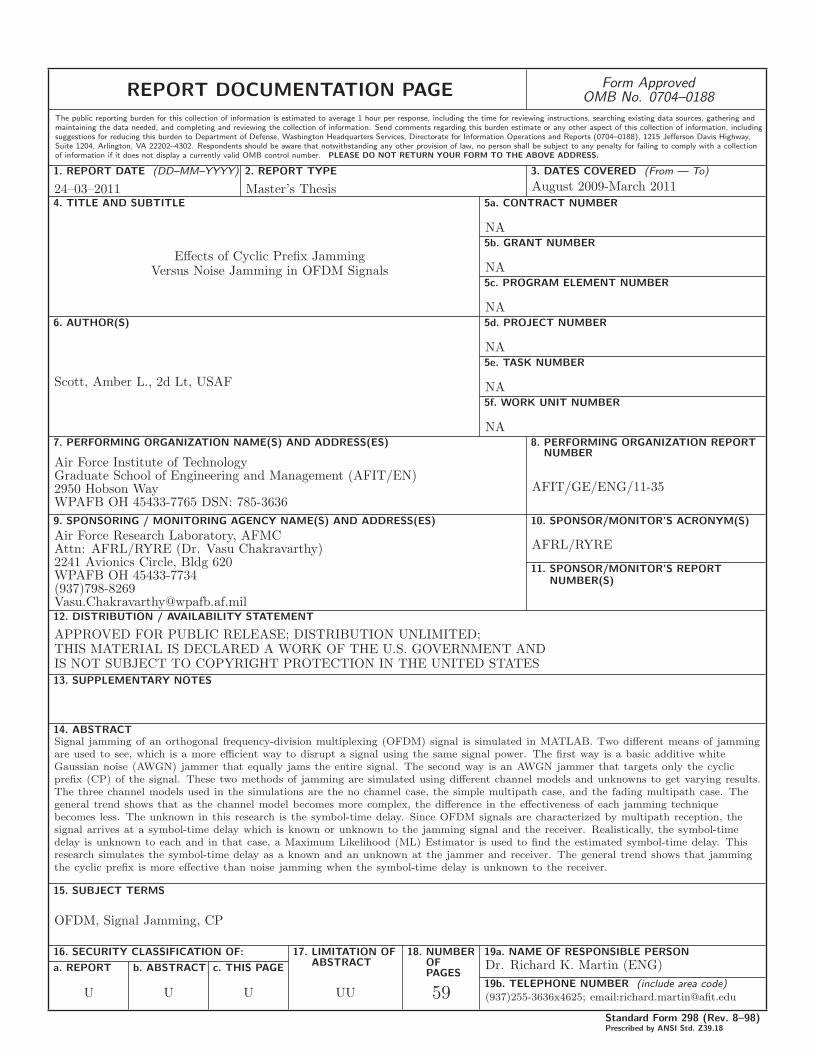
24–03–2011 Master’s Thesis August 2009-March 2011
Effects of Cyclic Prefix JammingVersus Noise Jamming in OFDM Signals
NA
NA
NA
NA
NA
NA
Scott, Amber L., 2d Lt, USAF
Air Force Institute of TechnologyGraduate School of Engineering and Management (AFIT/EN)2950 Hobson WayWPAFB OH 45433-7765 DSN: 785-3636
AFIT/GE/ENG/11-35
Air Force Research Laboratory, AFMCAttn: AFRL/RYRE (Dr. Vasu Chakravarthy)2241 Avionics Circle, Bldg 620WPAFB OH 45433-7734(937)[email protected]
AFRL/RYRE
APPROVED FOR PUBLIC RELEASE; DISTRIBUTION UNLIMITED;THIS MATERIAL IS DECLARED A WORK OF THE U.S. GOVERNMENT ANDIS NOT SUBJECT TO COPYRIGHT PROTECTION IN THE UNITED STATES
Signal jamming of an orthogonal frequency-division multiplexing (OFDM) signal is simulated in MATLAB. Two different means of jammingare used to see, which is a more efficient way to disrupt a signal using the same signal power. The first way is a basic additive whiteGaussian noise (AWGN) jammer that equally jams the entire signal. The second way is an AWGN jammer that targets only the cyclicprefix (CP) of the signal. These two methods of jamming are simulated using different channel models and unknowns to get varying results.The three channel models used in the simulations are the no channel case, the simple multipath case, and the fading multipath case. Thegeneral trend shows that as the channel model becomes more complex, the difference in the effectiveness of each jamming techniquebecomes less. The unknown in this research is the symbol-time delay. Since OFDM signals are characterized by multipath reception, thesignal arrives at a symbol-time delay which is known or unknown to the jamming signal and the receiver. Realistically, the symbol-timedelay is unknown to each and in that case, a Maximum Likelihood (ML) Estimator is used to find the estimated symbol-time delay. Thisresearch simulates the symbol-time delay as a known and an unknown at the jammer and receiver. The general trend shows that jammingthe cyclic prefix is more effective than noise jamming when the symbol-time delay is unknown to the receiver.
OFDM, Signal Jamming, CP
U U U UU 59
Dr. Richard K. Martin (ENG)
(937)255-3636x4625; email:[email protected]