Optimal Jamming against Digital ModulationSaiDhiraj Amuru, Student Member, IEEE, and R. Michael Buehrer, Senior Member, IEEE

Abstract—Jamming attacks can significantly impact the per-formance of wireless communication systems, and can lead tosignificant overhead in terms of re-transmissions and increasedpower consumption. This paper considers the problem of optimaljamming over an additive white Gaussian noise channel. Wederive the optimal jamming signal for various digital amplitude-phase modulated constellations and show that it is not alwaysoptimal to match the jammer’s signal to the victim signal inorder to maximize the error probability at the victim receiver.Connections between the optimum jammer obtained in thisanalysis and the well-known pulsed jammer, popularly analyzedin the context of spread spectrum communication systems areillustrated. The gains obtained by the jammer when it knows thevictim’s modulation scheme and uses the optimal jamming signalsobtained in this paper as opposed to conventional additive whiteGaussian noise jamming are evaluated in terms of the additionalsignal power needed by the victim receiver to achieve same errorrates under these two jamming strategies. We then extend thesefindings to obtain the optimal jamming signal distribution whena) the victim uses an OFDM-modulated signal and b) whenthere are multiple jammers attacking a single victim transmitter-receiver pair. Numerical results are presented in all the abovecases to validate the theoretical inferences presented.

I. INTRODUCTION

The inherent openness of the wireless medium makes itsusceptible to both intentional and un-intentional interference.Interference from neighboring cells in a wireless communi-cation system is one of the major causes for un-intentionalinterference. On the flip side, intentional interference corre-sponds to adversarial attacks on a victim receiver that is notoperating in a defensive mode. More generally, adversarialattacks in a wireless system can be broadly classified basedon the capability of the adversary- a) Eavesdropping attack,in which the eavesdropper (passive adversary) can listen tothe wireless channel and try to infer information (which ifleaked may severely compromise data integrity) [1], [2], [3],b) Jamming attack, in which the jammer (active adversary) cantransmit energy in order to disrupt reliable data transmissionor reception [4], [5], [6] and c) Hybrid attack, in which anadversary operates “with the dual capability of either passivelyeavesdropping or actively jamming any ongoing transmission,with the objective of causing maximum disruption to theability of the legitimate transmitter to share a secret messagewith its receiver” [7], [8].

In this paper, we study jamming attacks against practicalwireless signals, namely digital amplitude-phase modulatedsignals. Jamming has traditionally been studied in the contextof spread spectrum communications [9]. Barrage jamming,partial-band/narrow-band jamming, tone-jamming (where avictim is attacked by sending either a single or multiplejamming tones) and pulsed jamming are the most common

Parts of this paper have been presented at Globecom-2014 [10].The authors are with the Wireless@VT, Bradley Department of Electrical

and Computer Engineering, Virginia Tech, Blacksburg, VA 24061 USA (e-mail: adhiraj, rbuehrer@vt.edu).

types of jamming models considered in wireless communi-cation systems. Deviating from these traditional simplistictechniques, we want to know “What is the optimum statisticaldistribution for power constrained jamming signals in orderto maximize the error probability of digital amplitude-phasemodulated constellations?” As will be discussed in detailshortly, this paper answers a question that is more relevant topractical wireless communication systems when compared tosimilar questions studied in the past, and consequently offersdifferent solutions mainly because incorrect system modelswere previously considered and thus the wrong questions wereanswered.

Most of the earlier literature that asks similar questionsregarding optimal jamming signals can be divided into twocategories a) investigations that consider optimal jammingagainst Gaussian signaling schemes [4], [5], [6], [11], andb) investigations that study optimal jamming against pulseamplitude modulated (PAM) signals in the absence of ambientnoise [12], [13]. Typically, an information theoretic frameworkwas considered, e.g., [5], [6], [11], [13]. More specifically, in[5], the capacity of a wireless channel was analyzed in thepresence of correlated jamming, where the authors showed thatGaussian signaling and Gaussian jamming form a saddle pointsolution. Here, the authors also showed that when the jammerdoes not have knowledge regarding the phase and the timingoffsets introduced by the wireless channels, it is optimal interms of the capacity minimization to be uncorrelated withthe victim signal. In [6], [11], independent Gaussian inputand noise (jamming signal) signals were again shown to be asaddle point solution for the mutual information game betweenthe victim and the jammer. The convexity properties of errorprobability with respect to the AWGN jamming signal poweragainst a binary-valued victim signal was studied in [12],which showed that a pulsed AWGN jamming signal is optimal.In [13], the worst case performance, in terms of maximizingthe error probability and/or minimizing the capacity, achievedby any noise distribution was investigated when binary datawas transmitted. The optimal noise distribution was shown tobe a shifted version of the binary input signal.

Unfortunately, the previous works are not sufficiently real-istic. This is because the works that belong to category (a)consider jamming against Gaussian signaling which is notused in practice and the works that belong to category (b)ignore the presence of thermal/ambient noise which is typi-cally unavoidable in wireless environments. More importantly,these unrealistic assumptions lead to the wrong questions andthereby result in wrong conclusions, which are not relevantto practical wireless systems. The work closest to the presentstudy is [14] which studies the optimal power distribution forany given jamming signal, but does not address the questionraised in this paper. We show that optimal jamming sig-nals against digital amplitude phase modulated constellations

2

follow the statistical distribution of well-known modulationschemes under special conditions, and are not always matched(matching in this context refers to case where the jammer hasthe same distribution as the victim) to the victim signals. Thisfinding is in contrast to the results obtained in the previousworks.

In what follows, it is assumed that the victim receiver is notoperating in an anti-jamming mode. Such jamming scenarioscommonly occur because most transceivers do not employjamming detection algorithms. For such a victim receiver, thedecision regions for decoding the received signal will remainthe same irrespective of the presence or absence of a jammingsignal. For example, when the victim uses a symmetric binarysignaling scheme i.e., signal levels given by ±A where A isthe amplitude of signaling, and is unaware of the presence ofthe jammer, the decision boundary will still be 0. Improvedjamming techniques, such as the ones proposed in this paper,help military and/or practical wireless communication systemsjam their adversaries’ received signal before they can interpretany sensitive information.

We assume in this work that the jammer is aware of themodulation scheme of the communication signal (for example,by employing modulation classification schemes [15], [16])and also the power levels of the communication and thejamming signals at the victim receiver (using power controlinformation, location and/or path loss calculations). Theseassumptions enable us to analyze the worst case jammingperformance against standard modulation schemes. We firstshow that the optimal power-constrained jamming signalshares time only between two signal levels, i.e., the jammingsignal distribution takes the form of a binary distribution alongany signaling dimension (in-phase and quadrature). Further,it will be shown that this binary distribution is nothing butthe statistical distribution of well-known modulation schemesunder special conditions, and that it is not always the sameas the victim signal’s distribution. These results are thenextended to the more practical scenarios including (i) a non-coherent scenario where there is a phase mismatch betweenthe jammers’ signal and the victim signal, (ii) an asynchronousscenario where there is a timing offset between the jammers’signal and the victim signal and (iii) when the jammer is notperfectly aware of the power levels of the communication andjamming signals at the victim receiver.

We also extend this study to the cases where a) the victimtransmitter-receiver pair use an OFDM-modulated signal tocommunicate and b) when multiple jammers attack a singlevictim transmitter-receiver pair. Most previous works thatstudy jamming against OFDM signals consider AWGN jam-ming (see the tutorial paper [17] for more information), whichas we show in this work is sub-optimal in terms of the errorrates created at the victim receiver. Further, we show thatunder the same average power constraints i.e., the case wheremultiple jammers have the same total average power as a singlejammer, significantly higher error rates can be achieved whenthe multiple jammers are perfectly coordinated.

The rest of this paper is organized as follows. The systemmodel is introduced in Section II. The optimal jamming signaldistribution when the victim and the jammers’ signals are

phase and time aligned is derived in Section III. In Section IV,the jammers’ statistical distribution is derived for the caseswhen non-idealities are introduced by the wireless channeldue to which the jamming and the victim signals are notperfectly aligned. In Section V, we extend the analysis to thecase where the victim employs an OFDM modulated signaland in Section VI we study the performance of multiplejammers attacking a single victim transmitter-receiver pair.Numerical results are presented in sections III-VI to supportthe theoretical inferences made. Finally conclusions are drawnin Section VII.

II. SYSTEM MODEL

We assume that the data conveyed in the legitimate com-munication signal is mapped onto a known digital amplitude-phase constellation. The low pass equivalent of the transmittedsignal is represented as s(t) =

∑∞m=−∞

√PSsmg(t −mT ),

where PS is the average received signal power, g(t) is thereal valued pulse shape and T is the symbol interval. Thecomplex random variables sm denote the modulated symbols,with a uniform distribution fS(s), i.e., all possible constella-tion points are equally likely. Without loss of generality, theaverage energy of g(t) and modulated symbols E(|sm|2) arenormalized to unity.

It is assumed that the transmitted signal passes throughan AWGN channel (received power is constant over theobservation interval) while being attacked by a jamming signalrepresented as j(t) =

∑∞m=−∞

√PJjmg(t − mT ), where

PJ is the average jamming signal power as seen at thevictim receiver and jm denote the jamming symbols that aredistributed according to fJ(j) with E(|j|2) ≤ 1. Assuminga coherent receiver and perfect synchronization, the receivedsignal after matched filtering and sampling once per symbolinterval is given by

yk = y(t = kT ) =√PSsk +

√PJjk + nk, k = 1, 2, .. (1)

where nk is zero-mean additive white Gaussian noise whosedistribution is denoted by fN (n) with variance σ2. The victimsignal sk, the jamming signal jk and the noise samples nk areall assumed to be statistically independent of each other. LetSNR = PS

σ2 and JNR = PJ

σ2 indicate the signal power (PS) andjamming power (PJ) to noise power (σ2) ratios respectively.In this paper, we initially assume that the jammer has perfectknowledge of SNR and JNR as seen at the victim receiver.This assumption allows for the analysis of the maximum errorrates that can be created by the jammer at the victim receiver.We will later relax this assumption.

A. Motivation

Here, we briefly motivate the reason to look beyond AWGNjamming. Consider a BPSK signaling scenario with PS = 1,PJ = 1 and σ2 = 0 (i.e. the channel does not add any noise).Thus the received signal is expressed as

yk = sk + jk, k = 1, 2, . . . . (2)

If the jammer were aware of the signals sent by the transmitter,then it could negate them by sending the opposite of the

3

transmit signal, i.e., the jammer sends a −1 symbol to destroya +1 symbol. However, this is not possible in real time asthe jammer can not demodulate the transmit signal beforetransmission occurs. Hence, it sends a random BPSK signalto disrupt the communication. The receiver can decode thesymbols correctly half of the time i.e., when it gets ±2. Forthe other half of the time when it gets 0, it makes a randomguess regarding the transmit signal with probability 1

2 of beingcorrect. Thus the overall error probability is 1

4 = 0.25. Onthe other hand, the error probability is 0.1587 if an AWGNsignal (σ2 = 1) is used as the jamming signal [9]. For thistoy example, the BPSK modulated jammer increased the errorprobability by 57.5% as compared to the AWGN jammer(under similar power constraints) which suggests that thereare interesting avenues to pursue beyond AWGN jamming.

III. PERFECT CHANNEL KNOWLEDGE

First we analyze the statistics of the optimal jammer whenit has perfect channel knowledge i.e., the jamming signal isphase and time synchronous with the victim signal. In allthe analysis that follows, it is assumed that the receiver isunaware of the presence of the jammer and hence the decisionregions for the data detection remain the same as if therewere no jammer. We first derive the optimum jamming signaldistribution against a M -QAM1 victim signal and later showthat this can be simplified for specific modulation schemes.

For 2-dimensional signals, such as M -QAM, define yk =[<yk,=yk]T where <yk indicates the real (in-phase) part ofyk and =yk indicates the imaginary (quadrature) part of yk.Along similar lines we can define sk, jk and nk for all k =1, 2, . . . ,K. Then (1) is rewritten as

yk =√PS sk +

√PJ jk + nk, k = 0, 1, . . . ,K. (3)

Since the victim signal and the jammer’s signal are coherent,2-dimensional modulation schemes such as M -QAM can beanalyzed by considering them as two independent

√M -PAM

signals along the in-phase and quadrature dimensions [22].Therefore, the average probability of error2 pe of an M -QAMvictim signal along any signaling dimension in an AWGNchannel in the presence of jamming signal j is given by

pe(j,SNR, JNR) ≈

(1− 1√

M

)1

2×[

erfc

(√

SNRdmin

2+√

JNRj

)+erfc

(√

SNRdmin

2−√

JNRj

)],

(4)

where j = <j or =j, M is the order of the constellation anddmin is the minimum distance of the underlying modulationscheme [22].

The jammer intends to maximize this error probability bytransmitting a sequence of symbols j (along the in-phase and

1The analysis presented in this paper can also be extended to cross-QAMsignals by using the appropriate error probability expressions. But in thispaper, we focus on square QAM signals.

2With a slight abuse of notation, we use pe to denote the probability oferror. The variables that it depends on are shown within brackets. For example,pe(PS) indicates that pe is a function of the signal power PS .

the quadrature dimensions) which are to be chosen based onPS (or SNR) and PJ (or JNR). Notice that (4) is symmetricin j. Therefore, pe(j,SNR, JNR) = pe(−j,SNR, JNR) =pe(|j|,SNR, JNR). Hence, the polarity of j is irrelevanthere. Therefore, the error probability is maximized over thedistribution of a = |j|. However, to maximize the entropyof the jamming signal, transmitting a value of a, impliestransmitting j = +a and j = −a with equal probability.The optimization problem for such a jammer can thus beformulated as

maxfA

∫a

pe (a,SNR, JNR) fA(a)da s.t. E(a2) ≤ 1

2,

≡ maxfA

E(pe(a,SNR, JNR)

)s.t. E(a2) ≤ 1

2. (5)

Notice that the optimization is over the signal level distributionfA and that E(a2) ≤ 1

2 because we consider only onesignaling dimension (recall that E(||j||2) ≤ 1, where ||j||indicates the norm of the vector j).3 Similar optimizationproblems have previously been studied in the context ofstochastic signaling for maximizing the probability of signaldetection and minimizing the error probability in [14], [18],[19] and references therein. Below, we briefly present thesolution for the optimization problem in (5). A more elaborateand general proof for this optimization problem will be shownin Theorem 4 in Section VI, where we discuss the case ofmultiple jammers attacking a single victim receiver.

A. Optimum Jamming Signal DistributionDefine sets U and W as

U = (u1, u2) : u1 = pe (a,SNR, JNR) , u2 = a2

W = (w1, w2) : w1 = EfA

(pe (a,SNR, JNR)

), w2 = EfA(a

2).

Since pe (a,SNR, JNR) is a continuous function (erfc is acontinuous function) defined on the support of a, the mappingfrom [0, amax] (notice that it can be safely assumed that a ≤amax for some finite amax > 0 since arbitrarily large amplitudesof the signal cannot be generated by any practical transmitter)to (R+)2 defined by (pe (a,SNR, JNR) , a2) is continuous.Since the continuous image of a compact set is compact, theset U is also compact.

Since U is compact, the convex hull V of U is closed withdimensions smaller than or equal to 2 because U and V aresubsets of (R+)2. Based on the definition of the set W , it canbe shown that V = W [18, Proposition 3], [20] (an elaborateproof for this is given in Theorem 4). Further, Caratheodory’stheorem [21], states that any point in V can be expressedas a convex combination of at most three points in U as theybelong to (R+)2. Since the optimal jamming signal pdf shouldmaximize the objective function, the optimal solution exists onthe boundary i.e., on V (as it is a closed set). Since any pointon the boundary can be expressed as a convex combination ofat most 2 elements in U , the optimal jamming signal level pdffA(a) can be represented as a discrete random variable withat most 2 mass points.

3Depending on whether the victim’s modulation scheme is symmetric or notalong the in-phase and quadrature dimensions, this constraint can be changedaccordingly.

4

pe(λ, a1, a2,SNR, JNR) ≈

(1− 1√

M

)1

2

λ

[erfc

(√

SNRdmin

2+√

JNRa1

)+erfc

(√

SNRdmin

2−√

JNRa1

)]

+ (1− λ)

[erfc

(√

SNRdmin

2+√

JNRa2

)+erfc

(√

SNRdmin

2−√

JNRa2

)](7)

Since the above proof is generic for both the in-phaseand quadrature dimensions, the optimal jamming signal dis-tribution has at most two signal levels along any signalingdimension. Therefore the optimal jamming signal pdf alongany signaling dimension is given by

fA(a) = λδ(a− a1) + (1− λ)δ(a− a2), λ ∈ [0, 1]

λa21 + (1− λ)a2

2 ≤1

2, (6)

where λ and (1 − λ) are the probabilities with which thejammer sends signals a1 and a2 respectively along any dimen-sion and δ(a) is the Dirac-delta function. Thus, the problemof finding an optimum jamming signal distribution is nowreduced to finding λ, a1 and a2 rather than a continuousdistribution fJ(j) for the jamming signal j given in (3).

Remark 1: It is important to notice that this analysis holdstrue for any M -PAM and M -QAM signals because we startedthe analysis with the pe of an M -QAM signal by decomposingit into two

√M -PAM signals. Appropriate pe expressions

and average jamming signal energy constraints must be usedbased on the victim signal’s modulation. For example, theaverage jamming signal energy constraint E(a2) ≤ 1 for thecase of M -PAM signals as it is natural to consider jammingsignals only in the in-phase dimension against M -PAM signals(only then pe will be maximized) and E(a2) ≤ 1

2 for two-dimensional signals such as M -QAM.

B. Analysis against M -QAM victim signals

For the case of jamming against a M -QAM victim signal,it is not hard to show that pe(a,SNR, JNR) in (4) is a non-decreasing function of a and hence pe is maximized on theboundary defined by E(a2) = 1/2 (it is 1/2 because weconsider only one signaling dimension). Using the fact thatthe optimum jamming signal level distribution is given by (6),the overall pe along any signaling dimension is given by (7).

Numerically obtaining the optimal jamming signal distribu-tion under an average power constraint is difficult for a generalrange of SNR and JNR. Similar optimization problems havebeen solved using global optimization techniques such asparticle swarm optimization in [18]. In this paper, we firststate 3 theorems that help in establishing the optimal jammingsignal distribution against M -QAM victim signals for certainranges of SNR and JNR. Due to a lack of space, we onlysketch the proofs of these theorems. Later, we support theseclaims and present the optimal jamming signals for a generalrange of SNR and JNR via simulations performed usingthe optimization toolbox in Matlab. We also present severalremarks that help the exposition of these Theorems easier.

Theorem 1: QPSK is the optimal jammingsignal when the victim signal uses M -QAM and√

SNRd2

min

2 <√

JNR tanh(

2

√SNR

d2min

2 JNR)

.

Remark 2: Notice that tanh(

2

√SNR

d2min

2 JNR)≈1 when

SNRd2

min

2 JNR>1. Therefore, in this case, QPSK is the optimaljamming signal when SNR

d2min

2 <JNR which is a stricter con-

dition than√

SNRd2

min

2 <√

JNR tanh(

2

√SNR

d2min

2 JNR)

.

Remark 3: The theoretical pe when QPSK is used as ajamming signal is given by substituting a1 = 1√

2and λ = 1

in (7). The slope of the error probability with respect to SNR

i.e., ∂pe∂SNR within a proportionality constant when SNR

d2min

2 <

JNR and SNRd2

min

2 JNR > 1 can be approximated as

AWGN:−1√

SNR× JNR; QPSK:

−2√SNR× exp (JNR)

, (8)

which shows that the error probability due to a QPSK jammingsignal decays more slowly with JNR when compared to theAWGN jamming signal. Thus from a jammers’ perspective it isadvantageous to use a QPSK jamming signal when comparedto traditional AWGN jamming.

Proof: Since E(a2)= 12 , we have λa2

1 + (1 − λ)a22 = 1

2 .Using this relationship, (7) can be written as a function ofa1 denoted by pe(λ, a1,SNR, JNR). a1 = 0, 1√

2λ, 1√

2 are

the solutions to ∂pe(λ,a1,SNR,JNR)∂a1

=0. To prove the optimal-ity of QPSK, we need to show that pe(λ, a1,SNR, JNR)is maximized at a1= 1√

2(we will discuss the solutions

a1=0, 1√2λ

in Theorems 2 and 3). The second derivative

of pe with respect to a1 i.e., ∂2pe(λ,a1,SNR,JNR)∂a2

1|a1= 1√

2has

4 terms, each of which can be shown to be < 0 when√SNR

d2min

2 <√

JNR tanh(

2

√SNR

d2min

2 JNR)

. Further, thisholds true irrespective of a2 when a1= 1√

2and λ = 1. This

case is still in agreement with the optimal jamming signaldistribution because the proof of the optimal jamming signalpdf only says that the optimal jamming signal distribution canbe represented by a randomization of at most two differentsignal levels. Also recall that a = |<(j)| = |=(j)|. Thus,<(j) = =(j) = ± 1√

2.

From [23], it is well known that the entropy of any two-point distribution is maximized when each of the points isequally likely. Therefore the jammer sends a 1√

2symbol

on the in-phase or the quadrature dimension with prob-ability 1

2 and − 1√2

also with probability 12 . Therefore

the optimal jamming signal distribution is QPSK when√SNR

d2min

2 <√

JNR tanh(

2

√SNR

d2min

2 JNR)

.

5

√2SNRd2

minJNRexp

(− SNRd2

min

2

)<√

1− λopt

exp

(−

(√SNR

d2min

2−

√JNR

(1− λopt)

)2)

− exp

(−

(√SNR

d2min

2+

√JNR

(1− λopt)

)2), (9)

Theorem 2: a1, a2 =

0, 1√

2(1−λopt)

is the opti-

mal jamming signal along any signaling dimension when∂pe(λ,a1,SNR,JNR)

∂a1|a1=0 = 0 and ∂2pe(λ,a1,SNR,JNR)

∂a21

|a1=0 < 0

i.e., pe has a maxima at a1 = 0. λopt is obtained by solvingfor λ in the equation ∂pe(λ,a1,SNR,JNR)

∂λ |a1=0 = 0 and alsosatisfying (9).

Proof: As mentioned earlier, a1=0 is a solution for∂pe(λ,a1,SNR,JNR)

∂a1= 0. When this is true, the opti-

mal value of λ denoted by λopt is obtained by solving∂pe(λ,a1,SNR,JNR)

∂λ |a1=0 = 0. Further, it can be proved that∂2pe(λopt,a1,SNR,JNR)

∂a21

|a1=0 will be < 0 only when λopt satis-

fies (9). By symmetry

1√2λopt

, 0

is also a solution. Such a

solution is also known as on-off keying since the jammer sendspower using only one of the two possible signal levels, eithera1 or a2. Such a jamming signal will help to increase the pein cases where the jammer has limited power. The significanceof this solution will be explained in more detail shortly.

Remark 4: When on-off keying is optimal, it can be shownthat pe is equivalent to the probability of error achieved whenthe jammer uses QPSK signaling and either transmits withpower PJ

λoptor shuts off transmission with probability λopt and

(1−λopt) respectively. Such a jamming signal is equivalent toa pulsed jammer albeit modulated by a QPSK signal ratherthan AWGN [9], [24]. Exploiting this equivalence, we nextexplicitly characterize the range of SNR and JNR where on-off keying/pulsing is optimal.

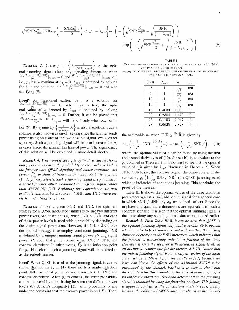
Theorem 3: For a given SNR and JNR, the optimumstrategy for a QPSK modulated jammer is to use two differentpower levels, one of which is 0, when JNR ≤ JNR, and eachof these power levels is used with a probability depending onthe victim signal parameters. However, if JNR > JNR thenthe optimal strategy is to employ continuous jamming. JNRis defined by a unique jamming signal power PJ and signalpower PS such that pe is convex when JNR ≤ JNR andconcave elsewhere. In other words, PJ is an inflection pointfor pe. Henceforth, such a jamming signal will be referred toas the pulsed-jammer.

Proof: When QPSK is used as the jamming signal, it can beshown that for the pe in (4), there exists a single inflectionpoint JNR such that pe is convex when JNR ≤ JNR andconcave elsewhere. When pe is convex, the error probabilitycan be increased by time sharing between two different powerlevels (by Jensen’s inequality) [23] with probability ρ andunder the constraint that the average power is still PJ . Then,

TABLE IOPTIMAL JAMMING SIGNAL LEVEL DISTRIBUTION AGAINST A 16-QAM

VICTIM SIGNAL, JNR = 10 dB.a1, a2 INDICATE THE ABSOLUTE VALUES OF THE REAL AND IMAGINARY

PARTS OF THE JAMMING SIGNAL.

SNR λopt a1 a2

-2 1 1√2

n/a4 1 1√

2n/a

10 1 1√2

n/a16 1 1√

2n/a

19 0.4633 1.039 022 0.2304 1.473 025 0.1193 2.047 028 0.0625 2.828 0

the achievable pe when JNR ≤ JNR is given by

ρpe

(1,

1√2,SNR,

JNR

ρ

)+(1−ρ)pe

(1,

1√2,SNR, 0

), (10)

where, the optimal value of ρ can be found by using the firstand second derivatives of (10). Since (10) is equivalent to thepe obtained in Theorem 2, it is not hard to see that the optimalvalue of ρ is given by λopt (discussed in Theorem 2). WhenJNR ≥ JNR i.e., the concave region, the achievable pe is de-scribed by pe

(1, 1√

2,SNR, JNR

)(the QPSK jamming case)

which is indicative of continuous jamming. This concludes theproof of the theorem.

Table III-B shows the optimal values of the three unknownparameters against a 16-QAM victim signal for a general casein which SNR R JNR (a1, a2 are defined earlier). Since thein-phase and quadrature dimensions are equivalent in such acoherent scenario, it is seen that the optimal jamming signal isthe same along any signaling dimension as mentioned earlier.

Remark 5: From Table III-B, it can be seen that QPSK isthe optimal jamming signal only until a certain SNR beyondwhich a pulsed-QPSK jammer is optimal. Further, the pulsingduration decreases as the SNR increases, which indicates thatthe jammer is transmitting only for a fraction of the time.However, it jams the receiver with increased signal levels inan attempt to compensate for the increased SNR. Notice thatthe pulsed jamming signal is not a shifted version of the inputsignal which is different from the results in [13] because wehave considered the effects of the additional AWGN noiseintroduced by the channel. Further, it is easy to show thatthe sign detector (for example, in the case of binary inputs) isno longer the maximum likelihood detector when the jammingsignal is obtained by using the foregoing analysis. This findingis again in contrast to the conclusions made in [13], mainlybecause the additional AWGN noise introduced by the channel

6

5 10 15 20 25 3010

−4

10−3

10−2

10−1

100

SNR

Ave

rag

e P

rob

ab

ility

of

Sym

bo

l E

rro

r

AWGN Pulse Jamming

Optimal Jamming

AWGN Jamming

16−QAM Modulation Jamming

QPSK Modulation Jamming

Maximum Entropy Jamming

Fig. 1. Comparison of various jamming techniques against a 16-QAMmodulated victim signal, JNR = 10 dB.

is also considered in the present work. However, notice that theoptimal maximum likelihood detection at the victim receiver inthe presence of jamming is not the focus of this present work.

The pe for the 16-QAM victim signal under various jam-ming scenarios is shown in Fig. 1. Here 16-QAM (QPSK)jamming refers to a randomly generated 16-QAM (QPSK)modulated jamming signal, and AWGN jamming refers to azero-mean white Gaussian noise jamming signal with variancePJ . It is well known that the entropy of a two-level distributionis maximized when λ = 0.5 [23]. A new optimization problem(extending the one in (5) and (6)) is solved by introducing anadditional constraint where λ = 0.5. We call such a jammingscenario as maximum entropy jamming. While maximum en-tropy jamming is better than QPSK jamming, it is worse thanthe optimal jamming as the constraint λ = 0.5 does not allowthe optimization algorithm to explore the pulsed jammingsolution. For a fair comparison, the jamming performance ofa pulsed jammer modulated with an AWGN signal [9] is alsoshown in Fig. 1. The optimal pulsing ratio λAWGN

opt for thepulsed AWGN jamming signal against any M -QAM victimsignal is obtained by using the first and second derivativeswith respect to λ of

(1− 1√

M

)[λerfc

(√SNR

(1 + JNRλ

)

dmin

2

)+ (1− λ)erfc

(√SNR

dmin

2

)].

AWGN-based pulsed jamming converts the exponentialrelationship between pe and SNR to a linear one [9]. Thisalso holds true for the case of the optimal jamming as seen inFig. 1. This is similar to the behavior of pe in a Rayleigh fadingchannel where it is inversely proportional to SNR. Intuitively,a symbol erased due to a deep fade is similar to the case wherea symbol is disrupted by jamming. Thus, the optimal jammeris capable of generating a fading channel-like scenario in anAWGN channel.

In summary, we first showed that the optimal jamming sig-nal distribution has a discrete distribution with only two masspoints along any signaling dimension. Specifically, we showedthat the signal levels of the in-phase or quadrature parts of thejamming signal will obey a two-point distribution. Using thisresult to address jamming against a M -QAM victim signal, wepresented three Theorems, where Theorem 1 shows that QPSK

is the optimal jamming signal against a M -QAM victim signal

when√

SNRd2

min

2 <√

JNR tanh(

2

√SNR

d2min

2 JNR)

, Theo-rems 2 and 3 show that pulsed QPSK is an optimal jammingsignal when JNR ≤ JNR. We used numerical optimizationtechniques to obtain a solution over all SNR, JNR, based onwhich it is conjectured that pulsed-QPSK is the optimal signalto jam any M -QAM modulated victim signal.

TABLE IIOPTIMAL JAMMING SIGNALS IN A COHERENT SCENARIO.

Victim signal Modulation scheme ofpulsed jamming signal

BPSK BPSKQPSK QPSK4-PAM BPSK

16-QAM QPSK

Remark 6: Since the two dimensional M -QAM constella-tions were analyzed by treating them as two orthogonal

√M -

PAM signals, the above analysis can be directly simplified forone dimensional signaling constellations such as BPSK, 4-PAM among others. Table II summarizes the optimal jammingsignals against commonly used digital amplitude-phase mod-ulated constellations. These results indicate that matching thejamming signal to the victim signal i.e., using the same signalas the victim is not always optimal.

IV. FACTORS THAT MITIGATE JAMMING

In this section, jamming is studied when the victim signalis not coherent (i.e., phase or time asynchronous) with thejamming signal when they reach the victim receiver. Froma jammers’ perspective, these non-idealities in the channel,specifically differences between the victim and jamming sig-nals will lower the impact of jamming at the victim receiver.For example, consider a scenario where the victim signal usesBPSK and the jammer also sends a BPSK signal. If the channelintroduces a 90 phase offset between these two signals, thenthe jammers’ signal does not have any impact on the victimsignal (as the receiver only demodulates the projections of thesignal received along the in-phase dimension).

If the phase/time shift between the victim signal and thejamming signal is known ahead of time to the jammer, itcan compensate for this in the jamming signal before it issent. However, this may be difficult to achieve in a real timecommunication system. Hence, in this section, we considerscenarios where the jammer is unaware of (or unable tocompensate for) this random phase or time offset introducedby the wireless channel and thus treats it as a random variable.From a jammers’ perspective it is necessary to optimize itssignal distribution across all random offsets introduced bythe channel. We also consider the case when the jammer isnot perfectly aware of the communication and jamming signalpower levels as seen at the victim receiver.

A. Non-Coherent Jamming

In this sub-section, jamming behavior is studied when thejammers’ signal is not coherent (i.e., phase asynchronous) with

7

pe(λ, j, SNR, JNR) ≈

(1− 1√

M

)1

2

[erfc

(√

SNRdmin

2+√

JNR(<j cos(φ)−=j sin(φ))

)+

erfc

(√

SNRdmin

2−√

JNR(<j cos(φ)−=j sin(φ))

)]. (13)

TABLE IIIOPTIMAL NON-COHERENT JAMMING SIGNAL LEVEL DISTRIBUTION

AGAINST A 16-QAM VICTIM SIGNAL, JNR = 10 dB. a1, a2 INDICATETHE ABSOLUTE VALUES OF THE REAL AND IMAGINARY PARTS OF THE

JAMMING SIGNAL.

SNR λopt a1 a2

-2 1 1√2

n/a4 1 1√

2n/a

10 1 1√2

n/a16 1 1√

2n/a

19 1 1√2

n/a22 0.185 1.642 025 0.094 2.304 028 0.049 3.211 0

the victim signal. With a random phase offset, the victim signalis given by

yk =√PS sk +

√PJexp (iφ) jk + nk, k = 0, 1, . . . ,K, (11)

where φ indicates the phase offset between the victim signaland the jamming signal at the victim receiver and is treated asa uniform random variable between 0 and 2π, and i =

√−1.

As in Section III, the optimization problem for the jammer isgiven by

maxfJ

EfJ

[Eφ

(pe (j, PS , PJ)

)]s.t. E(||j||2) ≤ 1. (12)

The optimal jamming signal distribution along any signalingdimension in the non-coherent scenario is obtained by follow-ing the analysis in Section III and is described below. Withoutloss of generality, we present the analysis for jamming againsta M -QAM victim signal as done in Section III.

Even in the non-coherent case, the M -QAM signal canbe analyzed by considering it as two orthogonal

√M -PAM

signals. However, in this case due to the random phase offsetbetween the jammers’ signal and the victim signal, projectionsof the jammers’ signal along each signaling dimension must beconsidered which is different from the analysis in Section III.The pe of a M -QAM signal along the in-phase dimensionwhen there is a jamming signal j and a random phase offsetφ, is given by (13). A similar expression holds true for thequadrature signaling dimension. Using (13) and solving theoptimization problem in (12) by following the analysis inSection III gives the optimal jamming signal level distributionshown in Table IV-A against a 16-QAM victim signal (weused the numerical optimization toolbox in Matlab to solvethe optimization problem). Even in this case a1, a2 indicatethe possible absolute values of the real and imaginary parts ofthe jamming signal j.

−5 0 5 10 15 20 25 3010

−4

10−3

10−2

10−1

100

SNR

Ave

rag

e P

rob

ab

ility

of

Sym

bo

l E

rro

r

AWGN Non−Coherent/Coherent Pulsed Jamming

QPSK Jamming

AWGN Jamming

Optimal Jamming, Non Coherent

Optimal Jamming, Coherent

Fig. 2. Comparison of jamming techniques against a 16-QAM victim signalin a non-coherent (random phase offset) scenario, JNR = 10 dB.

It is interesting to see that once again QPSK (recall that inthe coherent scenario, the optimal jamming signal distributionalong any signaling dimension was defined by ±a1 where a1

and −a1 are both transmitted with equal probability, the samedefinition holds true even in the non-coherent scenario) is theoptimal jamming signal until a certain SNR. Beyond this limit,pulsed-QPSK is the optimal jamming signal. This behavioris similar to the observations in Section III. When pulsing isoptimal, the non-zero signal level is given by its correspondingprobability as 1√

2λopt

or 1√2(1−λopt)

, which in other words

means that a QPSK modulated jammer with pulsing ratioλopt is the optimal jamming signal. In Table IV-A, notice thatthe optimization solver returned equal values for the jammingsignal levels along the in-phase and quadrature dimensions.This is due to the symmetry along these dimensions in thecase of 2-dimensional signaling which holds true irrespectiveof whether the jamming signal is coherent or non-coherentwith the victim signal.

Similar to the coherent scenario (see Theorem 3), pulsed-QPSK can be shown to be optimal when JNR ≥ JNR whereJNR is the inflection point of pe with respect to JNR. As thepresence of a phase offset reduces the jamming effect, JNR inthe non-coherent case is higher when compared to JNR in acoherent scenario. In other words, for a given JNR the SNR atwhich pulsing is optimal increases (as seen in Table IV-A) in anon-coherent scenario in comparison to the coherent scenariowhich was discussed earlier. The performance of the variousjamming signals against a 16-QAM victim signal is shownin Fig. 2. Although the pe achieved by the optimal jammingsignal (or pulsed-QPSK) is less when compared to the coherentscenario (due to phase mismatch), it is still higher than the peachieved using pulsed-AWGN jamming.

Similar to the coherent scenario, the analysis for the M -QAM constellations can be extended to any specific modula-

8

tion scheme in a non-coherent scenario. The optimal jammingsignals in such a phase asynchronous scenario against thecommonly used modulation schemes such as BPSK, 4-PAM,QPSK and 16-QAM are still given by Table II.4 However,the pulsed jamming duration of these optimal jamming sig-nals changes between the coherent and non-coherent (phaseasynchronous) scenarios as seen from Tables III-B and IV-A.As seen from Fig. 2, the gain in the SNR required to achievea target pe when compared to the coherent scenario, decreasesby 1-2 dB due to this phase mismatch.

B. Symbol Timing Offset

Similar to the phase offset, although the jammer identifiesthe modulation scheme and is aware of the symbol intervalused by the victim signal, it is difficult to be time aligned dueto the unknown delays introduced by the wireless channel.In this sub-section we consider the jamming performancewhen the victim signal and the jammers’ signal are not timesynchronized with each other. Note that, in general, phaseoffset and symbol timing offset can occur together in practicalwireless communication systems, but we do not consider boththese non-idealities together in this paper due to the complex-ity involved in optimizing the jamming signal. However, theframework developed thus far is still applicable and can beextended to such complex scenarios. Below, we focus on theeffects of timing offset on the jamming performance.

The low pass equivalent of the jammed victim signal aftermatched filtering is given by

yk =√PSsk +

√PJ

∞∑m=−∞

jmg(t−mT − τ) + nk,

k = 1, 2, . . . , (14)

where τ indicates the symbol timing offset/random delayintroduced by the channel, g(t) is a Nyquist pulse at the outputof the matched filter given by g(t) = g(t) ∗ g(t), where ∗indicates the convolution operation. For 2-dimensional signals,such as M -QAM, let yk = [<yk,=yk]T and along similarlines define sk, jk and nk for all k = 1, 2, . . . ,K. Then (14)is rewritten as

yk =√PS sk +

√PJ

∞∑m=−∞

jmg(t−mT − τ) + nk,

k = 1, 2, . . . , . (15)

By taking the pulse shape g(t) to be zero for |t| ≥MT (in fact,real implementations must truncate these pulses), the samplesykKk=1 are a function of the symbols jmM−1

i=−M+1.Since the jammer is unaware of the time delay introduced,

it treats the timing offset as a uniform random variable in theinterval τ ∈ [0, T ). Under such scenarios, the average pe of aM-QAM victim signal along any signaling dimension that the

4Even in the non-coherent scenario, BPSK continues to be the optimaljamming signal against any M -PAM signal. This is because a) only theprojections of the received signal along the in-phase dimension are usedto decode the victim signal and b) QPSK is a sub-optimal jamming signalbecause energy is wasted by transmitting along the quadrature dimension.

SNR0 5 10 15 20 25

Ave

rag

e P

rob

ab

ility

of

Sym

bo

l E

rro

r

10-2

10-1

100

Pulsed AWGN Jamming

Pulsed QPSK Jamming, τ=0

Pulsed QPSK Jamming, τ=0.2T

Pulsed QPSK Jamming, τ ∈ [0,T]

Fig. 3. Comparison of jamming techniques against a 16-QAM victim signalin the presence of timing synchronization errors, JNR = 10 dB.

jammer intends to maximize is given by

pe,τ,PAM (j, PS , PJ) =

(1− 1√

M

)1

2

∑j−M+1

. . .∑jM−1[

erfc

(√SNRdmin

2 +√

JNRj√

2

)+erfc

(√SNRdmin

2 −√

JNRj√

2

)],

where averaging is performed over all the ISI terms in order toevaluate the error rate and j indicates either the in-phase partor the quadrature part of

∑M−1m=−M+1 jmg(t−mT − τ). The

optimization problem that the jammer must solve to obtain theoptimal jamming signal distribution is given by

maxfJ

EfJ

[Eτ

(pe,τ,PAM

(j, PS , PJ

))]s.t. E(||j||2) ≤ 1,

(16)

where fJ indicates the jamming signal distribution. Even inthis scenario, the optimal jamming signal distribution can beshown to have two signal levels along any signaling dimension.However, it can be seen from (14)-(16) that the optimizationproblem in this scenario is more complicated compared to thecoherent and non-coherent scenarios due to the inter-symbolinterference (ISI) introduced by the incorrect sampling timeoffset. Hence, in this section, we study the performance of theoptimal jamming signal obtained in Section III in the presenceof a random time delay introduced by the wireless channel.

Fig. 3 shows the error rate performance of the optimaljamming signal in Table III-B against a 16-QAM victim signalin the presence of time synchronization errors (M = 2 anda roll-off factor of 0.65 for the raised cosine pulse shape).It is seen that the pe achieved by the jamming signal inTable III-B is lower as compared to the perfectly synchronizedscenario because of the ISI. However, it is seen that the peachieved by the jamming signal in Table III-B is still higherthan the pe achieved by the pulsed-AWGN jamming. Althoughthere may be specific cases where ISI helps the jammer toincrease the error rates by causing constructive interferenceagainst the victim signal, on an average the random time delayτ ∈ [0, T ] only reduces the impact of jamming (remember thatthe modulation-based jamming signal can still result in a lineardecay of the error rate with respect to SNR). This is because

9

the timing offset essentially creates a multiple level jammingsignal (the overall effect of ISI translates into this multi-leveleffect) which as we proved earlier is sub-optimal because atwo-level signal is the optimal jamming signal distribution.This explains the lower error rates achieved in comparisonto a perfectly synchronous case and seems to approach theperformance of an AWGN jamming signal (as seen in Fig. 3when τ ∈ [0, T ])

C. Signal Level Mismatch

When the jammer is not perfectly aware of the powerlevels of the communication and the jamming signals i.e.,PS and PJ at the victim receiver, the optimization problemspresented before in Section III do not result in the optimaljamming signal distribution. Due to this uncertainty, the errorrate performance of the jamming signals shown in Table III-Bwill be degraded. However, if the uncertainty in the knowledgeof PS or PJ is accounted for, then the jammer’s performancecan be significantly improved as will be shown below. Forease of analysis, we assume that the jammer is not aware ofPS exactly. Notice that the error in the knowledge of PJ canalso be accounted for along similar lines. If ε is the error inthe jammer’s knowledge about PS , then the jammer assumesthat the received signal at the victim receiver is given by

yk =√PS + εsk +

√PJ jk + nk, k = 0, 1, . . . ,K. (17)

To obtain the optimal jamming signal distribution under suchscenarios, the jammer solves the following optimization prob-lem;

maxfJ

EfJ

[Eε

(pe (j, PS + ε, PJ)

)]s.t. E(||j||2) ≤ 1. (18)

SNR-5 0 5 10 15 20 25 30

Ave

rag

e P

rob

ab

ility

of

Sym

bo

l E

rro

r

10-2

10-1

100

Pulsed AWGN - Exact Knowledge of ǫ

Pulsed QPSK - Ignore ǫ

Pulsed QPSK - Exact Knowledge of ǫ

Pulsed QPSK - Average over ǫ

Fig. 4. Comparison of jamming techniques against a 16-QAM victim signalin the presence of signal level mismatch, JNR = 10 dB.

Notice that this optimization problem is similar to theformulation in a phase-asynchronous scenario shown in (12).Thus, following the same principles as earlier, the optimaljamming signal can be shown to have a two-level distribu-tion along any signaling dimension. As before, we use theMatlab’s optimization toolbox to find the optimal jammingsignal distribution across all ranges of SNR and JNR. Fig. 4shows the performance of the optimal jamming signal incomparison to cases when the jammer is perfectly aware ofε and can therefore perfectly evaluate the optimal jammingsignal distribution at any given time instant. Also shown are

the performance of the pulsed AWGN and pulsed QPSKjamming signals when the jammer accounts for or ignoresthe error ε. Specifically, in Fig. 4, the error ε was taken to bedistributed as zero mean Gaussian with variance proportionalto the signal power PS and SNR = PS/σ

2. It is seen thatwhen the error is accounted for, the jammer can still performbetter than a) a pulsed QPSK jamming signal that ignored εand b) the naive AWGN jamming signal.

V. JAMMING AN OFDM SIGNAL

In this section, we study the optimal jamming signal distri-bution against OFDM-modulated wireless signals. The jammercan easily identify whether the victim is using a single-carrieror an OFDM-modulated signal by employing simple feature-based classification techniques [25]. Under such scenarios,we show that the optimal jamming signal is also an OFDMmodulated signal i.e., jamming in the frequency domain (bythis we mean that the jammer’s symbols are modulated ontothe sub carriers of the OFDM signal) is more effective incomparison to jamming in the time domain.

Typically, most earlier literature considered AWGN jam-ming signals to attack the victim (see the tutorial paper [17] formore information), but as we show below this is sub-optimal.This follows directly from the results presented in the previoussections in the context of a single carrier system. By usingthe optimal jamming signals obtained in this paper, innovativepower efficient jamming techniques such as cyclic prefixjamming, preamble jamming among others can be performed.However, this is not the major concern of this paper. In otherwords, we are concerned with jamming data only and notcontrol or synchronization parts of the victim’s transmission.For more information on efficient OFDM jamming attacks,please refer to [17].

In an OFDM system, an IFFT operation converts the fre-quency domain modulated symbols to time domain signalsbefore they are transmitted. The time domain OFDM symbols(l) is given by

s(l) =

Nsc∑k=1

S(k) exp(j2πlk/Nsc), ∀0 ≤ l ≤ Nsc − 1, (19)

where S(k) is the frequency domain signal/symbol which istypically a digital amplitude phase-modulated wireless signal,such as M -QAM and Nsc are the total number of sub-carriersused in the OFDM transmission. Assuming that the victimsignal passes through an AWGN channel (received power isconstant over the observation interval) while being attackedby a time-domain jamming signal j(l), the received signal atthe victim receiver is given by

y(l) =√PSs(l) +

√PJj(l) + n(l), (20)

where PS , PJ hold the same meaning as earlier. At thereceiver, the OFDM signal is passed through an FFT blockto recover the underlying frequency domain signal S(k) as

Y (k) =

Nsc−1∑l=0

y(l) exp(−j2πkl/Nsc)

10

Es/No, dB-5 0 5 10 15 20 25

Avera

ge P

robab

ility

of

Sym

bol E

rror

10-3

10-2

10-1

100

Time-Domain QPSK Jamming

Time-Domain AWGN Jamming

Frequency-Domain QPSK Jamming

Frequency-Domain AWGN Jamming

Frequency-Domain Pulsed AWGN Jamming

Frequency-Domain Pulsed QPSK Jamming

Frequency-Domain Pulsed QPSK Jamming, Non-Coherent

Fig. 5. Comparison of jamming techniques against a OFDM-modulated 16-QAM victim signal, JNR = 10 dB.

=√PSS(k) +

√PJ

Nsc−1∑l=0

j(l) exp(−j2πkl/Nsc) +N(k),

∀0 ≤ k ≤ Nsc − 1. (21)

Notice that (21) is similar to the single carrier scenariodiscussed before in the Section III. For instance, when S(k)is a M -QAM modulated victim signal, then based on theanalysis in Sections III and IV, the optimal jamming signalJ(k) =

∑Nsc−1l=0 j(l) exp(−j2πkl/Nsc) is a pulsed-QPSK

signal. Therefore, this leads to the conclusion that the opti-mal time-domain jamming signal j(l) is OFDM-modulatedwith frequency-domain symbols J(k), whose distribution wasobtained earlier in Sections III, IV. Thus, all the findings ofthe earlier sections in the context of a single carrier systemcan also be extended to the case of OFDM signaling.

Fig. 5 shows the performance of the various jamming sig-nals against OFDM-based 16-QAM modulated victim signal.Specifically, each OFDM symbol consists of 64 subcarrierswith data modulated on only 52 subcarriers. Further, a cyclicprefix of length 16 was appended to each OFDM symbolin the simulations. Notice that the time-domain AWGN andQPSK jamming signals achieve the same error rates becausethe QPSK signal will also look similar to an AWGN signalafter the FFT operation at the victim receiver. It is also seenthat frequency domain jamming (with the same structure asthe victim signal i.e., 64 subcarriers with data modulated ononly 52 subcarriers and a cyclic prefix of length 16) performssignificantly better than time domain jamming and also thefrequency domain pulsed QPSK jamming signal achievesa higher error rate than all other jamming signals. Thesefindings are in agreement with the results discussed earlierin Section III. Also shown is the performance of the pulsedQPSK jammer when the victim signal and the jamming signalare non-coherent i.e., there is a phase-offset between thesesignals at the victim receiver. In this case, the optimal jammingsignal is obtained by following the steps in Section IV-A. Theperformance of the optimal jamming signal even in this caseis similar to that of the single carrier system.

It is well-known that frequency offset is a major problemin OFDM signals in comparison to the timing offset. This isbecause the presence of a cyclic prefix helps overcome theeffects of a timing offset introduced by the wireless channel.

Es/No, dB0 5 10 15 20 25

Sym

bo

l E

rro

r R

ate

10-2

10-1

100

Frequency Domain Pulsed QPSK Jamming, frequency offset = 0

Frequency Domain Pulsed QPSK Jamming, frequency offset = 0.1

Frequency Domain Pulsed QPSK Jamming, frequency offset ∈ [0,1]

Frequency Domain Pulsed AWGN Jamming, frequency offset ∈ [0,1]

Fig. 6. Comparison of jamming techniques against a OFDM-modulated 16-QAM victim signal in the presence of a frequency offset, JNR = 10 dB.

Moreover the effects of the frequency offset in OFDM-basedsignals can be related to the effects of a timing offset in singlecarrier systems. Therefore, the jamming performance in thepresence of a frequency offset between the victim and thejamming signals can be related to the timing asynchronouscase in a single carrier system which was discussed beforein Section IV-B. A frequency offset between the jammingand the victim signal leads to inter-carrier interference (ICI),which similar to ISI in a single carrier system, degradesthe performance of the jamming signal with respect to theerror rates created at the victim receiver. Since optimizingthe jamming signal in the presence of a frequency/timingoffset is complex due to the presence of ICI/ISI, we study theperformance of the jamming signal obtained in the coherentscenario when it is used in the presence of a frequency offset.

When the jamming and the victim signals are off byan integer number of subcarrier spacings, the orthogonalitybetween the subcarrier’s of the jammer and the victim signalsremains intact due to the cyclic shift created by the receiver’sFFT operation. Thus no ICI is created in this case and the per-formance would be similar to that shown in Fig. 5. Hence, onlya fractional frequency offset, i.e., offsets less than a subcarrierspacing, are considered in this analysis. Fig. 6 shows the errorrates achieved by the jamming signal when the jamming andthe victim signal are frequency asynchronous. As expected, theerror rate performance is degraded in comparison to the casewhen the jamming and the victim signals are perfectly alignedin terms of the frequency. Note that the performance of theAWGN jamming signal will also be affected by a frequencyoffset unlike the case when their performance is not impactedby a phase offset between the jamming and the victim signals.

VI. THE CASE OF MULTIPLE JAMMERS

In this section, we analyze the error rates achieved by multi-ple coordinating jammers attacking a single victim transmitter-receiver pair. It is assumed that the total average poweravailable with the multiple jammers is the same as the averagepower available with a single jammer that was studied in theprevious sections. When the jammers are coordinated, theycan jointly evaluate the optimal joint jamming signal distri-bution that maximizes the probability of error at the victimreceiver. We show the superior performance of such a joint

11

optimal jamming signal distribution by comparing it againstthe cases where multiple jammers are un-coordinated andhence employ the optimal single jamming signal distributionsobtained in previous sections. Further, these increased errorrates can be achieved by using only lower average powerlevels at each jamming node which also helps in reducingthe jammer detection probability. The assumption that thejammers can coordinate enables us to evaluate the maximumpossible error rates that can be created at the victim receiverunder a given average power constraint. In scenarios, wheresuch coordination is not possible, alternate techniques such asonline learning [26]-[28] can be employed. In this paper, werestrict to the cases where coordination between the multiplejammers is possible, for example by communicating via a sidechannel.

The received signal at the victim receiver when N coherentand synchronous jammers attack a single victim signal s, isgiven by

yk =√Pssk +

N∑i=1

√PJ(i)ji,k + nk, k = 1, 2, . . . ,K (22)

where yk, sk, nk were defined earlier and ji,k indicates thejamming kth jamming symbol sent by the ith jammer such thatE(||ji||2) ≤ 1. Here, PJ(i) is the power of the ith jammingsignal at the victim receiver and

∑i PJ(i) = PJ , i.e., the total

average power available with the multiple jammers is the sameas available with a single jammer considered in the previoussections. For ease of exposition, we show the analysis for theoptimal jamming signal along any one signaling dimensionwhich can be easily extended to any dimension i.e., to considerany standard modulation schemes following the analysis donein the previous sections.

By letting ji indicate the in-phase or the quadrature partsof the jamming signal, the pe along any signaling dimensionfor an M -QAM signal, is given by (4) by replacing j in(4) with

∑Ni=1

√PJ(i)ji. Since ji indicates either the in-

phase or the quadrature components of the jamming signal,we have the following average power constraint E(j2

i ) ≤ 12 .

Hence, when the jammers can coordinate and try to maximizethe error rate at the victim receiver, they solve the followingoptimization problem to obtain the optimal jamming signalalong any signaling dimension,

maxE(pe(j1, . . . , jN )) s.t. E(j2n) ≤ 1

2, n = 1, 2, . . . , N.

where the expectation is taken with respect tofj1,j2,...,jN (j1, . . . , jN ), which denotes the joint optimaljamming signal distribution of all the jammers that intend toattack the victim.

Remark 7: When the jammer’s cannot coordinate with eachother, then the joint jamming signal distribution along anyone signaling dimension fj1,j2,...,jN (j1, . . . , jN ) is given by∏Ni=1 fJi(ji), where the jamming signal distribution for the

ith jammer fJi(ji), is given by the optimal single jammerdistribution derived earlier in Sections III-V. We show that thisresults in a sub-optimal jamming performance when comparedto scenarios where the jammer’s can coordinate.

The following theorem establishes the structure of the jointoptimal jamming signal distribution fj1,j2,...,jN (j1, . . . , jN )along any signaling dimension.

Theorem 4: The joint optimum jamming signal distributionfj1,j2,...,jN (j1, . . . , jN ) along any signaling dimension, whenN jammers attack a single victim transmitter-receiver pair isdefined by N + 1 levels.Proof: Define set U as

U =

(u1, u2, u3, . . . , uN+1) : u1 = pe(j1, j2, . . . , jN ),

un+1 = j2n, ∀n = 1, 2, . . . , N

(23)

Since pe is continuous, the mapping defined by(pe(j1, j2, . . . , jN ), j2

1 , j22 , . . . , j

2N ) is also continuous in

the domain |jn| ≤ jmax, ∀n = 1, 2, . . . , N , where jmax

indicates the maximum signal level that can be sent bythe jammers. Such an assumption is common for wirelesscommunication systems because arbitrarily large signal levelscannot be generated by practical transmitters.

Now, U is a compact set, because the continuous image ofa compact set is also compact. Let V represent the convexhull of U . Since U is compact, V is closed with dimensionsnot exceeding N + 1 as it is a subset of (R+)N+1.

Now, define a set W as

W =

(w1, w2, w3, . . . ,WN+1) :

w1 =

∫ ∫pe(j1, j2, . . . , jN )fj1,j2,...,jNdj1dj2 . . . djN ,

wn+1 =

∫ ∫j2nfj1,j2,...,jNdj1dj2 . . . djN ,

∀n = 1, 2, . . . , N, (24)

where fj1,j2,...,jN (j1, . . . , jN ) is the joint pdf of the jammingsignals used by the coordinated jammers. Notice that theelements of W are the expected values of the elements of U ,where expectation is taken with respect to the joint jammingsignal distribution fj1,j2,...,jN .

It is known from previous results that, if a random variableΘ takes values in a set Ω, then its expected value E(Θ) takesvalues in the convex hull of Ω [20], [29, Appendix 4.B]. Thisindicates that W is in the convex hull V of the set U . In otherwords, we have W ⊆ V .

We will now show that V ⊆ W . Since V is the convexhull of U, each element inside V can be easily expressed asv =

∑L`=1 λ`(pe(j

(`)1 , j

(`)2 , . . . , j

(`)N ), j

(`)1 , j

(`)2 , . . . , j

(l)N ) with∑

` λ` = 1 and λ` > 0. Here j(`)i indicates the `th point of

the the jamming signal ji. See that set W has an elementequal to v for fj1,j2,...,jN =

∑L`=1 λ`δ(j − j(`)) where

j = (j1, j2, . . . , jN ) and j(`) = (j(`)1 , j

(`)2 , . . . , j

(`)N ). Therefore,

every element of V is also a subset of W which leads toV ⊆W . Using the above two results we have, V = W .

By using the Caratheodory’s theorem [18], we have that anypoint inside V or W can be expressed as a convex combinationof at most L = N + 2 points that belong to U . Now sincethe jammers intend to maximize pe, the optimal value lies onthe boundary of V which can be expressed by at most N + 1elements that belong to U . Thus the optimal pdf fj1,j2,...,jN is

12

described by N+1 vectors namely (j(`)1 , j

(`)2 , . . . , j

(`)N )N+1

`=1

such thatN+1∑`=1

λ`(j(`)n )2 ≤ 1

2, ∀n = 1, 2, . . . , N. (25)

This concludes the proof of the Theorem.Remark 8: When a single jammer attacks a victim receiver,

i.e., the case of N = 1 given in (22), then Theorem 4 givesthe result mentioned earlier in Section III-A regarding theoptimality of a two-level jamming signal distribution alongany signaling dimension.

By following the procedure in Section III, and using thestructure of the optimal jamming signal distribution in Theo-rem 4, we obtain the error rates against standard digital ampli-tude phase modulated victim signals. By following the analysisin Section IV, the optimum jamming signal distribution in thepresence of non-idealities in the channel can also be obtained.Numerical results that show the performance of the multiplejamming signals is discussed next.

A. Results

Fig. 7 shows the error rates achieved by various jammingtechniques when N jammers attack a single victim node. Inall the cases, the overall average power used by the jammersis restricted to PJ in order to compare with the error rateperformance of a single jammer and each jammer has equalpower equal to PJ

N . It is clearly seen that unless both thejammer’s coordinate, the gains in pe are not achievable. Bycoordinate, we mean that the jammers should pulse at thesame time when pulsing is optimal i.e., all the jammers shouldtransmit at the same time by employing the optimal jointjamming signal distribution (which in this paper is obtained byusing the optimization toolbox in Matlab). It is worth noticingthat a 3dB SNR gain is achieved when the number of jammersis doubled i.e., 3dB higher SNR is required at the victim toattain the same error rate.

When coordination is not possible, the multiple jammerperformance is limited and it can only achieve the error ratesachieved by a single jammer. Notice that in the ranges whereQPSK jamming is optimal for a single jammer, the errorrates achieved by two un-coordinated jammers is degraded.This is because a positive signal sent by one jammer can becancelled by a negative signal that may be sent by the other un-coordinated jammer. However when the jammers are pulsing,the probability that their pulsing instants may match is on theorder of ρ2 (ρ being the pulse jamming probability) which issmall, and hence there is a small probability that their signalsmay cancel each other. This is why the error rates achievedby the un-coordinated jammers in the pulsing region matchesthe error rate achieved by a single jammer. As expected, theperformance of all these jamming signals is better than thenaive AWGN jamming signal.5 Also shown is the performanceof the optimum jamming signal distribution when the jammersare non-coherent (phase offset between the signals) when theirsignals reach the victim receiver. As expected the performance

5Note, that the performance of multiple pulsed AWGN jammers willcoincide with the performance of a single pulsed AWGN jamming signal.

of the joint optimal non-coherent jamming signal is degradedin comparison to the coherent case.

SNR-5 0 5 10 15 20 25 30

Ave

rag

e P

rob

ab

ility

of

Sym

bo

l E

rro

r

10-1

100

1 Jammer, Pulsed QPSK

1 Jammer, Pulsed AWGN

2 Jammers, un-coordinated, Pulsed QPSK with PJ/2

2 Jammers, Optimal Joint Signal Distribution

2 Jammers, Optimal non-Coherent Joint Signal Distribution

4 Jammers, Optimal Joint Signal Distribution

Fig. 7. Comparison of jamming techniques when multiple jammers attack asingle 16-QAM modulated victim signal, JNR=10dB.

VII. CONCLUSION

In this paper, we characterized the optimal statistical distri-bution for power-constrained jamming signals that jam digitalamplitude-phase modulated constellations in an AWGN chan-nel in both single carrier and OFDM-based wireless systems.The analysis in this paper shows that modulation-based pulsedjamming signals are optimal in both coherent and non-coherent(phase asynchronous) scenarios. As opposed to the commonbelief that matching the victim signal (correlated jamming)increases confusion at the victim receiver, our analysis showsthat the optimal jamming signals match standard modulationformats only in a certain range of signal and jamming powers.Beyond this range, either binary or quaternary pulsed jammingis the optimal jamming signal. An interesting relationshipbetween these optimal jamming signals and the well-knownpulse jamming signals discussed in the context of spreadspectrum communications was illustrated. As expected, theperformance of these optimal jamming signals was seen tobe degraded when the victim and the jamming signals arenot phase or time synchronous or when it does not haveperfect knowledge of the power levels of the victim andthe jamming signals although the optimal jamming signaldistributions don’t change. Against OFDM-based signaling, itwas observed that OFDM-based jamming signals that use theoptimal jamming signal distributions obtained in single carrierscenarios are optimal and that their performance is degraded inthe presence of channel non-idealities such as residual carrierfrequency offset. Upon extending this analysis to a multiplejammer scenario, it was found that gains in terms of theerror rate at the victim receiver are possible only when themultiple jammers are perfectly coordinated, otherwise multiplejammers can only match the impact of a single jammer. Theoptimal jamming signal distributions against practical wirelesssignals that employ error correction coding techniques is beinginvestigated.

REFERENCES

[1] A. D. Wyner, “The wire-tap channel,” Bell System Technical Journal,vol. 54, no. 8, pp. 1335-1387, Jan. 1975.

13

[2] I. Csiszar and J. Korner, “Broadcast channels with confidential messages,”IEEE Trans. Inf. Theory, vol. 24, no. 3, pp. 339-348, May 1978.

[3] Y. Liang, H. V. Poor, and S. Shamai (Shitz), “Information theoreticsecurity,” Foundations and Trends in Communications and InformationTheory, vol. 5, no. 7, pp. 355-580, 2008.

[4] T. Basar, “The Gaussian test channel with an intelligent jammer,” IEEETrans. Inf. Theory, vol. 29, no. 1, pp. 152-157, Jan. 1983.

[5] M. Medard, “Capacity of correlated jamming channels,” in Proc. AnnualAllerton Conf. Commun. Control and Comput., Monticello, IL, 1997,pp. 1043-1052.

[6] A. Kashyap, T. Basar, and R. Srikant, “Correlated jamming on MIMOGaussian fading channels,” IEEE Trans. Inf. Theory, vol. 50, no. 9,pp. 2119-2123, Sept. 2004.

[7] A. Mukherjee and A. L. Swindlehurst, “Jamming games in the MIMOwiretap channel with an active eavesdropper,” IEEE Trans. Signal Pro-cess, vol. 62, no. 1, pp. 82-91, Jan. 2013.

[8] Y. O. Basciftci, C. E. Koksal and F. Ozguner, “To Obtain or not to ObtainCSI in the Presence of Hybrid Adversary,” arXiv:1301.6449, Jan. 2013.

[9] M. K. Simon, J. K. Omura, R. A. Scholtz, and B. K. Levitt, SpreadSpectrum Communications, vol. 1. Rockville, MD: Comput. Sci. Press,1985.

[10] S. Amuru and R. M. Buehrer, “Optimal Jamming Strategies in DigitalCommunications-Impact of Modulation,” in Proc. Global Commun. Conf,Austin, TX, Dec. 2014, pp. 1619-1624.

[11] R. McEliece and W. Stark, “An information theoretic study of commu-nication in the presence of jamming”, in Proc. Int. Conf. Commun., 1981,pp. 45.3.1-45.3.5.

[12] M. Azizoglu, “Convexity properties in binary detection problems,” IEEETrans. Inf. Theory, vol. 42, pp. 1316-1321, Jul. 1996.

[13] S. Shamai (Shitz) and S. Verdu, “Worst-Case Power Constrained Noisefor Binary-Input Channels,” IEEE Trans. Inf. Theory, vol. IT-38, no. 5,pp. 1494-1511, Sep. 1992.

[14] S. Bayram et al. “Optimum power allocation for average power con-strained jammers in the presence of non-Gaussian noise,” IEEE Commun.Lett., vol. 16, no. 8, pp. 1153-1156, Aug. 2012.

[15] S. Amuru and C. R. C. M. da Silva, “Cumulant-based channel estimationalgorithm for modulation classification in frequency-selective fadingchannels,” in Proc. IEEE Military Comm. Conf., Orlando, FL, 2012, pp.1-6.

[16] S. Amuru and C. R. C. M. da Silva, “A blind pre-processor for mod-ulation classification applications in frequency-selective non-Gaussianchannels,” IEEE Trans. Commun., vol. 63, no. 1, pp. 156-169, Jan. 2015.

[17] C. Shahriar et al., “PHY-Layer Resiliency in OFDM Communications:A Tutorial,” IEEE Commun. Surv. and Tut., vol. 17, no. 1, pp. 292-314,Mar. 2015.

[18] C. Goken, S. Gezici, and O. Arikan, “Optimal stochastic signalingfor power-constrained binary communications systems,” IEEE Trans.Wireless Commun., vol. 9, no. 12, pp. 3650-3661, Dec. 2010.

[19] B. Dulek and S. Gezici, “Detector randomization and stochastic signal-ing for minimum probability of error receivers,” IEEE Trans. Commun.,vol. 60, no. 4, pp. 923-928, Apr. 2012.

[20] L. Huang and M. J. Neely, “The Optimality of Two Prices: MaximizingRevenue in a Stochastic Communication System,” in IEEE/ACM Trans.Netw., vol. 18, no. 2, pp. 406-419, Apr. 2010.

[21] A. W. Roberts and D. E. Varverg, Convex Functions. New York:Academic Press, 1973.

[22] J. G. Proakis and M. Salehi, Digital Communications, 5th ed. New York:McGraw-Hill, 2008.

[23] T. M. Cover and J. Thomas, Elements of Information Theory, 2nd ed.New York: Wiley, 2006.

[24] R. A. Poisel, Introduction to Communication Electronic Warfare Sys-tems. Artech House, 2008.

[25] M. Shi, A. Laufer, Y. Bar-Ness, and W. Su, “Fourth order cumulants indistinguishing single carrier from OFDM signals,” in Proc. IEEE MilitaryCommun. Conf., San Diego, CA, Nov. 2008, pp. 1-6.

[26] S. Amuru and R. M. Buehrer, “Optimal Jamming using DelayedLearning,” in Proc. Military Commun. Conf., Baltimore, MD, Oct. 2014,pp. 1528-1533.

[27] S. Amuru, C. Tekin, M. van der Schaar, and R. M. Buehrer, “ASystematic Learning Method for Optimal Jamming,” in proc. Intern. Conf.Commun. (ICC), London, UK, Jun. 2015.

[28] S. Amuru, C. Tekin, M. van der Schaar, and R. M. Buehrer, “JammingBandits,” in arXiv preprint arXiv:1411.3652, Nov. 2014.

[29] M. J. Neely. “Dynamic Power Allocation and Routing for Satelliteand Wireless Networks with Time Varying Channels.” PhD thesis,Massachusetts Institute of Technology, Laboratory for Information andDecision Systems (LIDS), 2003.