effects of leading-edge ice accretion geometry on airfoil...

(c)l999 American Institute of Aeronautics & Astronautics

A99-33388 AIAA-99-3150

EFFECTS OF LEADING-EDGE ICE ACCRETION GEOMETRY ON AIRFOIL PERFORMANCE

Han S. Kim* Michael B. Bragg+

University of Illinois at Urbana-Champaign

ABSTRACT

A systematic study of the effect of simulated ice shape geometry on airfoil aerodynamics was performed. A wind tunnel test was performed using a flapped NLF( l)-0414 airfoil where aerodynamic parameters including hinge moment were measured. The ice shapes tested were designed to simulate a single glaze ice horn with leading-edge radius, size and airfoil surface location varied. In all nine ice simulations were tested at six different leading edge locations. The objective of this research was to determine the sensitivity of iced airfoil aerodynamics to ice shape geometry. Configurations were also tested at three different Reynolds numbers (0.5, 1.0, and 1.8~10~). It was determined that ice horn leading-edge radius had only a small effect on airfoil aerodynamics. However, the aerodynamic performance was very sensitive to ice shape size and location. An almost linear relationship between loss in maximum lift and ice horn location was found with the largest loss at the furthest location back on the upper surface. Reynolds number was found to have little effect on the aerodynamic results on the airfoil with simulated ice shapes.

INTRODUCTION

The term “critical ice accretion” is typically used to describe the one ice formation that is believed to cause the maximum degradation in aircraft performance. Critical ice accretions are currently used in the aircraft

certification process. However, to accurately determine the critical ice accretion for an airfoil, the relationship between ice geometry, airfoil geometry, and corresponding performance degradation must be determined. This understanding is currently lacking. Determining this relationship also has other benefits, such as incorporating this relationship in the design phase of an airfoil or wings of an aircraft to minimize the sensitivity to icing. Also, the understanding of ice geometry vs. performance degradation may assist in improving the accuracy of computational models. This information will help determine when an ice shape is predicted with enough fidelity to properly simulate the aerodynamic effects of an actual ice accretion.

Large ice accretions effectively alter the gross airfoil geometry. The performance degradation trends consistent with large ice accretion can also be observed in variations in airfoil geometry. These effects of airfoil geometry are well documented by Hoemer and Borst.’ The data presented as a function of nose radius, camber, and other variables, document their effect on airfoil aerodynamics and performance.

Taking a simplistic view of large ice accretion on airfoil geometry, the accretion can cause an increase in camber, changes in the airfoil nose radius, thickening of the airfoil, etc. Hoemer shows in detail the relationship between the parameters of an airfoil and their resulting performance effects. He states that leading-edge radius primarily determines the stall type and the C, mar of an airfoil. Sharp leading edges generally result in thin airfoil or leading-edge stall, with lower C, ma values.

l Graduate Research Assistant, Department of Aeronautical and Astronautical Engineering, Member AIAA. t Professor and Head, Department of Aeronautical and Astronautical Engineering, Associate Fellow ALU.

Copyright 1999 0 by Han S. Kim and Michael B. Bragg. Published by American Institute of Aeronautics and Astronautics, Inc. with permission.

379

When the nose radius reaches about 1.5 to 2.0% of the chord, an optimum C,,, results for most airfoils.

c I mm and stall are also a function of camber. Hoemer states that camber allows laminar separation and the “bubble-plus-reattachment” mechanism to be minimized. He also states that these effects are relatively independent of the Reynolds number. Increases in camber generally result in corresponding increases in C,,, until the camber becomes too great. So the effects of variations in camber resemble the effects of varying leading-edge radii. These effects correlate well to the effects of icing, which generally lisplay losses in C, mar and changes in stall types. However, it is important to note that this is a very simplistic view of large ice accretion, since the effect of ice accretion on the flowfield can not be simplified to just a gross variation in airfoil geometry.

Weick and Scudde? studied the effects of sharp leading edges on a Clark Y airfoil by attaching two different sharp leading-edge shapes. The tests showed that the sharp leading edges caused a slight reduction in ‘drag, a change in stall type from a trailing edge stall to a more thin airfoil stall, and approximately 13% loss in ~C, max. They also mention a similar Gottingen 398 test imat showed a 26% decrease in C, ,,,aT and a small ,negative lift curve slope post stall.

~ Ingehnan-Sundberg, Trunov and Ivan&o’s analysis

#provided a good starting point for this research. In their Fit joint report, they tested various ice accretion shapes and sizes on a four-element, one-meter chord ‘wing section, and on a 0.65-meter chord NACA i65zA215 airfoil. They list the effects of large ice ‘accretion on the airfoil flow:

1 1. Extracts kinetic energy from the boundary I layer which promotes separation. 1 2. Causes increased local friction drag. / 3. Reduces pressure recovery at the trailing I edge. ; 4. Changes the wing section (effectively a

geometry change of the wing section) and directly affects the pressure field.

The data showed that even the smallest ice accretion dramatically lowered the C, -. They also noted that !decrease in C, mnx with respect to size was nonlinear.

I

I 380


The data also suggested that the shape of the ice accretion and the surface condition of the airfoil had the most impact on the airfoil performance degradation, with rime ice shapes generally having less effect than horn-shaped ice of similar size. They also noted that the effects on C, - and Cd of ice accretion just on the lower surface was much less than when the accretion was placed on both upper and lower surfaces. The C,,, loss was between 20 - 40% for cases with no trailing- edge devices and the C, mnx loss never exceeded 25% when trailing-edge devices were deployed. This study did not however discuss the effect of varying ice shape locations.

Ingelman-Sundberg and Tru.tro~~~~ showed large increases in elevator hinge moment caused by the redistribution of the pressure forces on the airfoil in their second and third joint report. Similar increases in hinge moment are thought to have caused numerous accidents, including the ATR-72 commuter aircraft accident of 1994 where the ice accretion caused a large hinge moment on the aileron.6.

Mullins, Smith and Korkan’ showed that the chordwise location of residual ice shapes had a significant effect on the laminar bubble separation extent and reattachment. They also noted that separation without reattachment occurred when the ice shape was placed closer to the leading edge (xic less than 10% chord on a NACA64AOlO with WC < 2.5%). This indicates that slight variations in the leading-edge geometry can have significant effects on the flowfield. They also suggested that adverse pressure gradients and the extent of laminar flow play an important part in airfoil performance in icing conditions.

Recent tests by Lee, et al.,8 also show the importance of the chordwise position of an accretion representing a supercooled large droplet (SLD) accretion. A forward facing quarter round (.25”, WC = 0.0139) was tested on a modified NACA 23012 airfoil at varying chordwise locations. The iced cases showed a change in stall characteristics, dramatic reductions in C cmm and large increases in drag, However, the worst case occurred when the simulated ice was near x/c = 0.10, where C, mnx decreased to 0.3 (80% decrease) compared to 0.56 for x/c = .02 (62% decrease), and 0.42 for x/c = 0.2 (72% decrease). The NACA23012 has a clean C, mM of 1.4 at Re=l.5x106 and 1.48 at


Re=l.8x106. The x/c = 0.10 case also showed the worst drag increase and the lowest astil of just 6”. The pitching moments were also heavily dependent on the chordwise position.

Much of aircraft icing aerodynamics research to date has been limited by the lack of a clear understanding of the relationship between geometric parameters of ice accretion and their corresponding performance penalties. It is often though that ice shapes that are similar in size but of different geometry can have vastly differing effects on airfoil performance. Also, current belief is that when an accretion grows sufficiently large, any additional increase in size no longer has an effect on the C, ,,,=. It is desired to investigate the aerodynamic effects caused by these large ice accretions in order to explain or contradict these assumptions. Understanding the relationship between ice accretion geometry and the resulting aerodynamic penalty is also important in establishing procedures to determine the most critical ice accretion geometry. This experimental study focuses primarily on the relationship between airfoil leading-edge ice geometry (ice accretion height, horn radius, and location) and aerodynamic performance.

EXPERIMENTAL SETUP

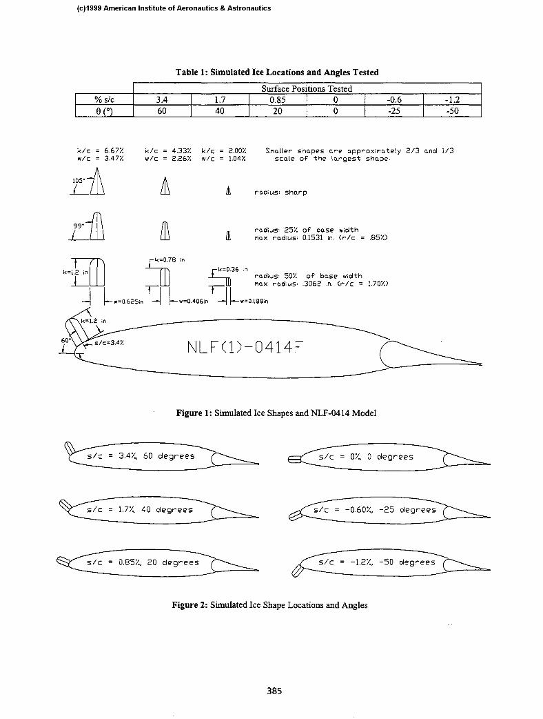
A scaled drawing of the simulated ice and the model is shown in Fig. 1. An 1 g-inch chord NLF( l)- 0414 was used for this research. The simulated ice shapes were machined out of aluminum and attached to the model via model end plates and secured with tape. For the larger shapes, the gaps between the base of the simulated ice shapes and the surface of the model were filled with plastina (modeling clay). The simulations maintained constant size and shape over the entire span. The simulated ice was tested in 3 sizes: k = 1.2” (k/c = 6.67 %), k = 0.8" (k/c = 4&I%), and k = 0.4” (k/c = 2.22%). The simulated ice shapes were tested at six different surface locations. The locations and horn angles are shown in Fig. 2. The ice shapes were attached normal to the surface at those locations. It can be seen in Table 1 that the locations were chosen so that each subsequent location doubles the horn angle and doubles the distance for both upper and lower surfaces. The horn angle was measured from the model chord

line to the line connecting the mid point of the base to the tip of the ice simulation. The simulated ice geometries were determined from averaging geometry data from a set of actual ice accretions collected from a test at the NASA Lewis Icing Research Tunnel. Due to geometric differences between the upper and lower surface ice, only upper surface ice accretion geometries

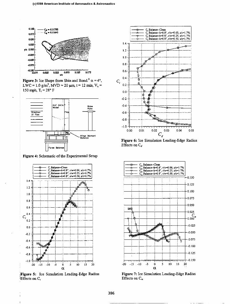
were simulated for this research, although these geometries were also tested at two lower surface locations. As of this writing no two-horn (both upper and lower horns) configurations have been tested, but these tests will be conducted in the near future. The ice shapes used can be found in Shin and Bond’ and an example is given in Fig. 3.

The research was performed in the UIUC 3 x 4 ft. wind tunnel. Figure 4 shows the schematic of the experimental setup. Each configuration was tested at two Reynolds numbers (1.0 x lo6 and 1.8 x 106) and 3 flap settings (-So, O”, and 5”). C, and C, about c/4 were mainly taken from the force balance and Cd values were calculated primarily from the wake although force balance data were also collected. Surface pressure measurements were taken over areas which were not covered by the ice simulations, and C,, was calculated from a hinge moment load cell and surface pressure. Figure 4 shows the experimental setup. Florescent oil flow-visualization tests were also performed to determine and verify flow characteristics. All data shown are corrected for tunnel wall effects via methods described in Rae and Pope.”

RESULTS AND DISCUSSION

Siinulated Ice Leadiw-EdPe Radius Figure 5 shows the C, vs. a curves for k = 0.8” and

s/c = 1.7% with varying horn tip radii. The ice simulations cause the C,, to decrease from the clean value of 1.35 to about 0.76 (C,, = 0.79 for r/w=.5, C, - = 0.75 for r/w = 0). Figure 6 shows the C, vs Cd curves from the same data set as Fig. 5. A drag increase for the airfoil with simulated ice shapes can clearly be observed when compared to the clean case, but the simulated ice horn leading-edge radius has negligible effect on the data. All three ice shapes show a Cdmi,, value of about 0.014 (at C, = .6) compared to .007 (at C, = 0.68) for the clean airfoil, and the curves

381


for the three ice shapes are virtually identical. Figure 7 shows the C, vs a curves for the same data set. Again it can be observed that the affect of the simulated ice leading-edge radius plays only a small role in determining airfoil performance parameters. The I . addmon of the ice shapes caused the airfoil to have a more nose up pitching moment (increase in C,) but the magnitude of this change was not affected by the ice simulation leading-edge radius.

The magnitude of the ice simulation leading-edge radius effect varied slightly with position and height. p leading-edge radius effects were most pronounced near and post stall for larger simulated ice shapes and bositions further away from the leading edge. The /sharper shapes (lower r/w) displayed lower C,,, values lbut generally lower Cdmin values as well. Leading-edge radius effects on C, were also minimal. As shown in ‘Figs. 5, 6, and 7, the magnitude of the differences were iless than 5% of the average values at a point. I

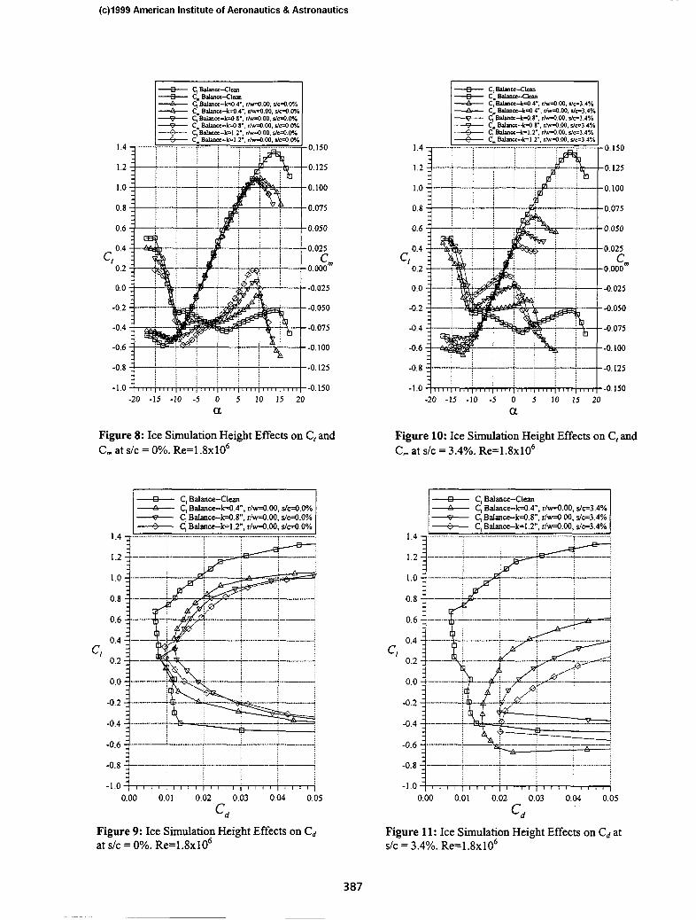
/Simulated Ice Height I The effect of height was strongly dependent on the isurface position of the simulated ice. Figures 8 and 9 ,show the C, , C,, and Cd curves with the simulated ice ,at s/c = 0% and Re=1.8x106 and Figs. 10 and 11 show ~the same at s/c = 3.4%. As shown in Fig. 8, height Ivariations near the leading edge did not cause any appreciable change in C, mM which remains near 1.1 regardless of height variations (C, mar = 1.12 for k = ‘0.4”, c,,, 1.09 fork = 0.8”, C,,, = 1.10 fork = 1.2”). The same is true for aSroll which remains near a = 9”- 10”. However, it can be seen that there is a large

iincremental change in C, caused by the variation in ‘height, with the moment increasing as the ice height increases for 0” < a < 10”. Near a = 9” the k = 1.2” shape shows C, = -. 005, k = 0.8” shows C, = -.013,

1 and k = 0.4” shows C,,, = -.03 1. This is probably due to the changes in the flowfield and the effective

~lengthening of the airfoil chord due to presence of the ~ ice shape. Extending the leading edge increases the ice shape moments and this coupled with the larger force on the larger shape increases the C, about the quarter

I chord location. This is also unusual since changes in C- m generally indicate changes in the flowfield which are

’ also reflected in C, However, this is not the case here as seen in the two figures.

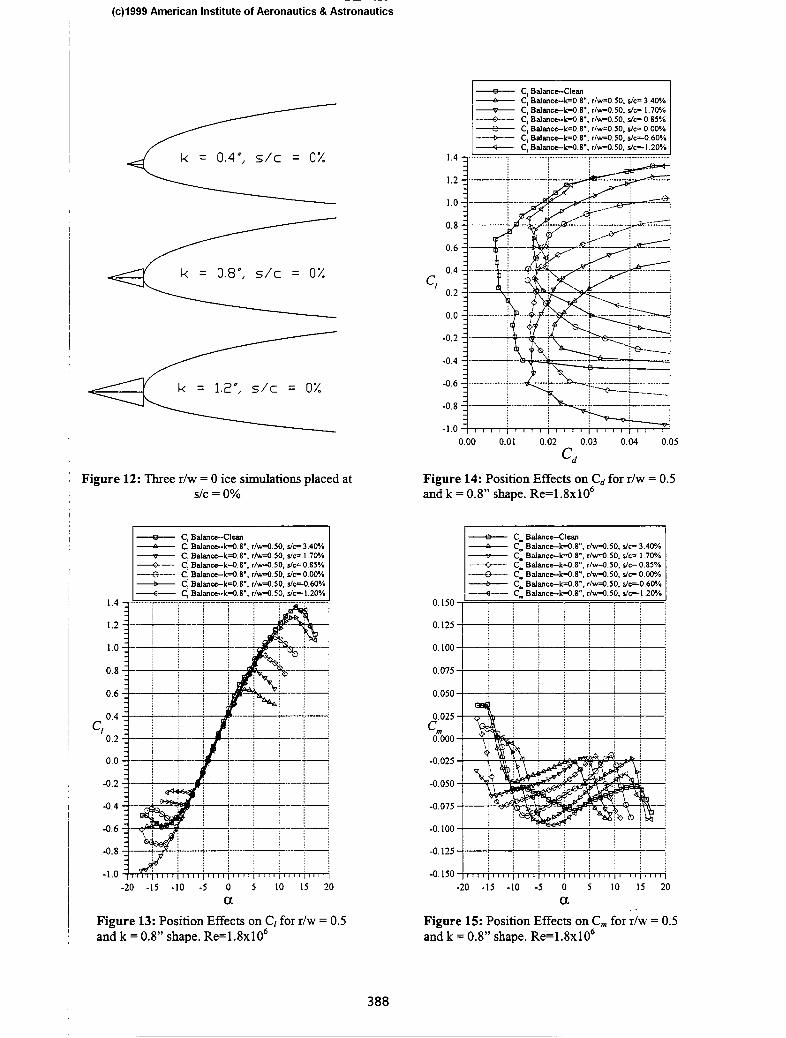
It’s also interesting to note that the Cdmin for the largest and smallest shape (k = 0.4” and 1.2”) are less than that for the medium size shape (k = 0.8”) although the overall Cd values are in logical order at higher a’s. This may be due to the base width of the ice shape. The k = 0.4” shape’s base width account for only a fraction of the airfoil’s thickness near the leading edge, which accounts for it’s negligible effect on drag. The k = 1.2” shape is very close to the thickness of the airfoil near the leading edge which allowed the gap between the base of the ice shape and the airfoil to be sealed relatively smooth (essentially acting as a fairing). For the k = 0.8” shape, this was not the case. This probably caused a separation bubble to form which altered the local and possibly the global flowfield. A drawing of the three shapes in this configuration can be seen in Fig. 12.

At s/c = 3.4%, the height makes a significant difference in C,,, and a,I,I1 as shown in Fig. 10. With k = 1.2”, the C, ,,,m = .43 and aStall = l”, which is only about 32% of the clean C,,, and 12” less than the clean aStQll. The k = .8” and k = .4” shapes show C,,, values of .56 and .72, respectively and aJIoll values of 3” and 5”, respectively. It is interesting to note that the although the angle at which the peaks in C, occur are very different from s/c = O%, the magnitude of the change in C, in Fig. 8 are similar to the magnitudes seen at Fig. 10. Figure 10 also seems to show a change in stall type from the trailing-edge stall type of the clean configuration to a more thin-airfoil stall type for the simulated ice configurations. Figure 11 shows that Cd increases roughly proportional to height, but Cd,,,, for k = 0.8” and 1.2” were the same with a value of Cdmin = .02 (although they occur at different C’s).

Simulated Ice Surface Position As implied previously, surface position plays a

critical role in the aerodynamic performance degradation due to icing. Effects of varying surface positions on C, Cd, C,, and C,, are given in Figs. 13, 14, 15 and 16. It can be seen that larger s/c locations cause a larger decrease in C,,, and lower a,d as compared to the clean case. CT,,, values in Fig. 13 are 1.36, 1.26, 1.09, 0.93, 0.80 and 0.63 (ice shape locations/c= -1.2% to 3.4% listed in increasing s/c) compared to 1.35 for the clean case. When attached to the lower surface, the

I 382


simulated ice provided slightly higher than the clean positive C, - values with the simulated ice essentially acting as a leading-edge flap. It also should be noted that as ice shape location s/c increases, the Cdmin values occur at lower C, ‘s or lower a’s

Figure 14 shows that Cdmin z .016 for all S/C

locations except for the s/c = 3.4% position which had Cdmin = .021, which was unexpected. All ice shape locations produced Cdmin values higher than clean values. However, as shown in Fig. 9, Cdmin values close to the clean values are possible. It also should be noted that as s/c increases, the C&in values occur at lower C, ‘s and lower a’s. These results seem to support the idea that iced airfoil drag is lowest at the angle of attack the ice was accreted at (ai&. It also suggests that the vicinity of s/c = 3.4% may represent the limit as to what can be categorized as a “leading-edge” ice accretion for this airfoil. A similar effect has been seen in other research with SLD shapes.’ This point has important implications and need additional research.

Figure 15 shows that the C, values near positive stall for ice simulations occur at fairly even increments of a as s/c decreases from 3.4% to 0%. The breaks occur with a difference of 2” to 3” between these cases. C, values for the upper surface iceshape locations at a’s near positive stall remain fairly constant with C, z - .02. C, quickly decreases with an increase in a after stall to create a more nose down pitching moment. A similar angle effect occurs for the negative stall region in the cases where the ice simulations are placed on the lower surface (s/c 5 0) although the magnitude of C, decreases as the ice simulation is moved further aft on the lower surface.

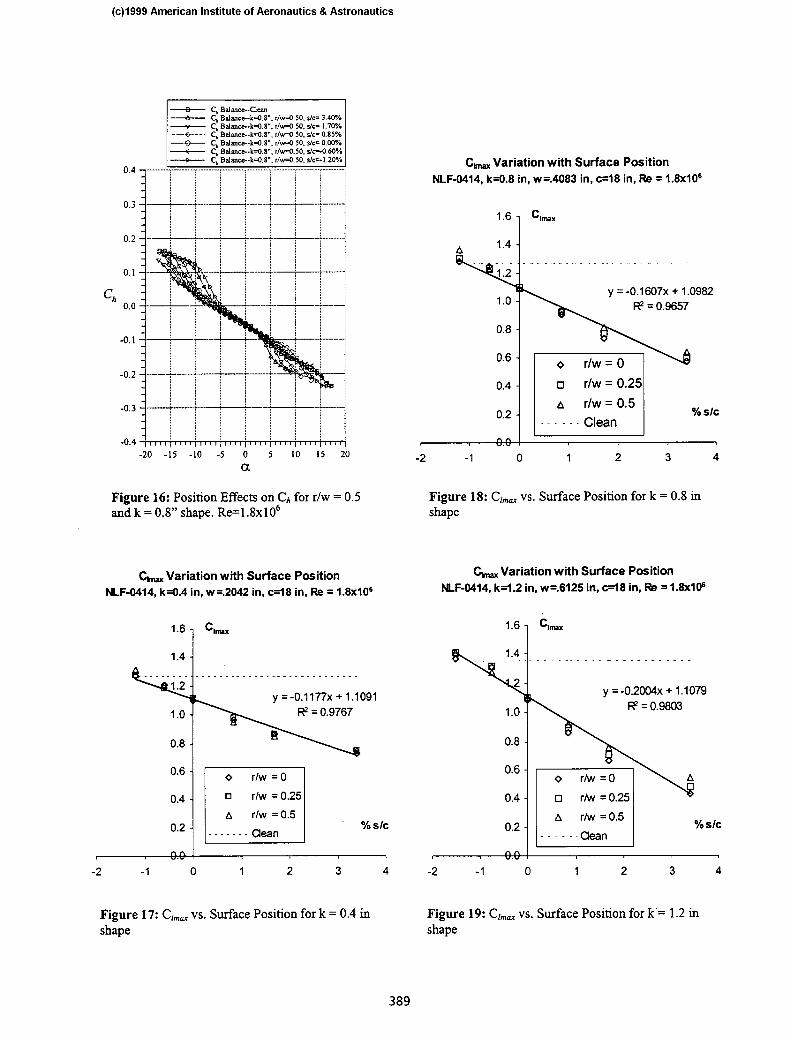
Figure 16 shows that the Ch values with simulated ice remain similar to clean configuration values until a approaches a,,II. Ch slightly increases above clean values just before stall and then sharply decreases below clean values after stall causing a sharp flap trailing edge up moment. For example, with simulated ice placed at the s/c = 0% location, C,, = -0.12 at a = 7" compared to the clean configuration value of Ch = - 0.14. At as,II = lo”, the two values become similar as the hinge moment for the iced configuration becomes more negative (clean configuration C,, = -0.16, simulated ice Ch = -0.156). At a = 12”, the simulated ice Ch = -0.20 compared to clean configuration value of

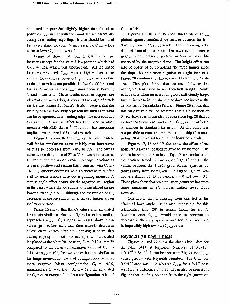
c*= -0.164. Figures 17, 18, and 19 show linear fits of C, -

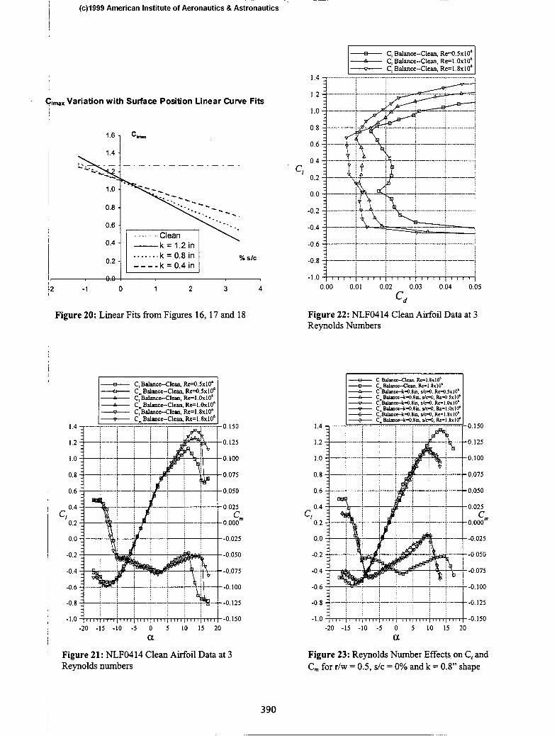
plotted against simulated ice surface position for k = 0.4”, 0.8” and 1.2”, respectively. The line averages the data set from all three radii. The incremental decrease in Grm with increase in surface position can be readily observed by the negative slope. The height effect can also be observed by comparing the three figures since the slopes become more negative as height increases. Figure 20 combines the linear curve fits from the 3 data sets. This plot shows that s/c near 0.4% exhibit negligible sensitivity to ice accretion height. Some believe that when an accretion grows sufficiently large, further increase in ice shape size does not increase the aerodynamic degradation further. Figure 20 shows that this may be true for ice accreted near a s/c location of 0.4%. However, it can also be seen from Fig. 20 that at s/c locations near 3.4% and -1.2%, C,,, can be affected by changes in simulated ice height. At this point, it is not possible to conclude that the relationship illustrated in Fig. 20 is universal for other ice horns on airfoils.

Figures 17, 18 and 19 also show the effect of ice horn leading-edge location relative to s/c location. The values between the 3 radii on Fig. 17 are similar at all s/c locations tested. However, on Figs. 18 and 19, the values between the 3 radii grow further apart as s/c moves away from s/c = 0.4%. In Figure 19, s/c=3.4% shows a AC,,,,, of .15 between r/w = 0 and r/w = 0.5. These plots show that ice simulation geometry becomes more important as s/c moves further away from s/c=O.4%.

One factor that is missing from this test is the effect of horn angle. It is also impossible for this relationship (Fig. 20) to remain linear for all s/c locations since C, mar would have to continue to decrease as the ice shape is moved further aft resulting in impossibly high (or low) C,,, values.

Revnolds Number Effects Figures 21 and 22 show the clean airfoil data for

the NLF 0414 at Reynolds Numbers of 0.5x106, l.0x106, 1.8~10~. It can be seen from Fig. 21 that C,,, varies greatly with Reynolds Number. The C, mar for 0.5~10~ case was 1.12 whereas C,,, for 1.8~10~ case was 1.35; a difference of 0.23. It can also be seen from Fig. 22 that the drag polar shifts to the right (increased

383


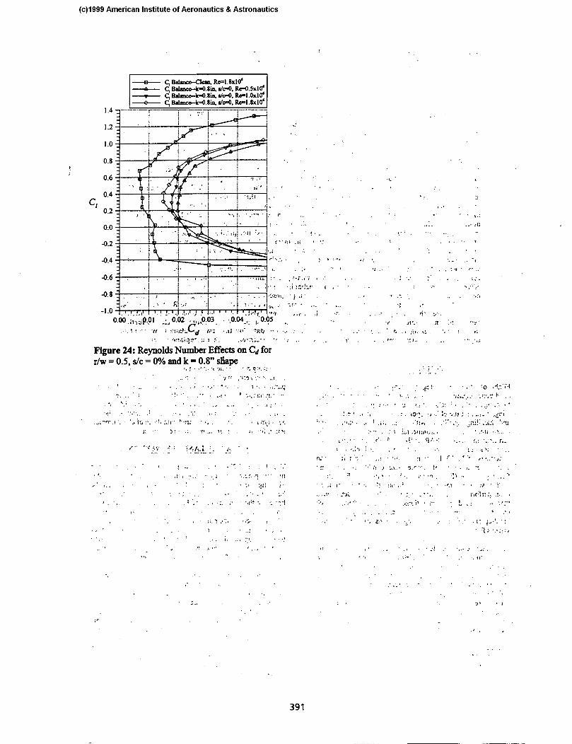
drag at the same lift coefticient) with decreasing Reynolds Number. With the addition of simulated ice, the Reynolds Number effect was greatly reduced. This can be seen in Figs. 23 and 24. Figure 23 shows that C, and C, between the three Reynolds Numbers tested are virtually identical. The C, - for 0.5~10~ case was 1.10, :l.0x106 case was 1.12, and for 1.8~10~ case was 1.09; a maximum difference of 0.03. Therefore, AC, max between clean and iced configurations may vary with Reynolds Number, but the actual C,,, of the ice shape can be reproduced correctly at least within this Reynolds Number range.

CONCLUSIONS

The results to date indicate that ice surface location ,combined with ice horn height play a crucial role in jdeterminin g iced airfoil performance degradation. It ialso seems that the size of the ice accretion, even when lsufficiently large, does not alone determine the :“critical” ice shape. Specific conclusions are:

Simulated ice shape size and location had a significant effect on the measured reduction of C and other measures of aerodynamic pL*Y-ce. The relationship between surface location and C near the leading edge (x/c c 3.5%) is fin; linear with AC, mar increasing as the ice shape is placed further aft on the airfoil upper surface. C I,- dependence on ice simulation height and radius was a minimum at s/c = 0.4% Reynolds Number had little effect on the C,,, of the airfoil with simulated ice horns. Radius effects are largest for large horns at large s/c locations but are small compared to size and location effects. Drag results seem to support the idea that iced airfoil drag is lowest at the angle of attack the ice was accreted at (aid). Drag results also suggest that the vicinity of s/c = 3.4% may represent the limit as to what can be categorized as a “leading-edge” ice.

Acknowledpment This research was supported by the National

Aeronautics and Space Administration (NASA) under grant NAG 3-1988. The authors would also like to gratefully acknowledge Mr. Sam Lee for assisting during the testing phase of this research.

References:

’ Hoemer, S. F. and Borst, H. F. Fluid-Dvnamic Lift, Hoemer Fluid Dynamics, Brick Town, N.J., 1975.

’ Weick, Fred and E. Scudder, Nathan F., ‘The Effect on Lift, Drag, and Spinning Characteristics of Sharp Leading Edges on Airplane Wings”, NACA TN 447, February 1933.

3 Ingelman-Sundberg, M., Trunov, O.K. and Ivan&o, A., “Methods for Prediction of the Influence of Ice on Aircraft Flying Characteristics”, a joint report from the Swedish-Soviet Working Group for Flight Safety, 6” Meeting, 1977.

4 Ingehnan-Sundberg, M. and Tnmov, O.K. “Wind Tunnel Investigation of the Hazardous Tail Stall Due to Icing”, a joint report from the Swedish-Soviet Working Group for Flight Safety, 1979.

’ Ingelman-St&berg, M. and Trunov, O.K. “On the Problem of Horizontal Tail Stall Due to Ice”, a joint report from the Swedish-Soviet Working Group for Flight Safety, 1985.

6 Bragg, M.B. “Aircraft Aerodynamic Effects Due to Large Droplet Ice Accretions”, AIAA 96-0932, January 1996.

’ Mullins, B. Jr., Smith, D., and Korkan, K. “Effects of icing on the Aerodynamics of a Flapped Airfoil”, AIAA 95-0449, January 1995.

’ Lee, S., Dunn, T., Gurbacki, H. M., Bragg, M. B., and Loth, E., “An Experimental and Computational Investigation of Spanwise-Step-Ice Shapes on Airfoil Aerodynamics”, AIA4 98-0490, January, 1998.

9 Shin, Jaiwon, and Bond, Thomas H., “Repeatability of Ice Shapes in the NASA Lewis Icing Research Tunnel”, Journal ofAircraft, Vol. 31, No. 5, Sept-Oct. 1994.

lo Rae, W. H. and Pope, A., Low-Sueed Wind Tunnel w, John Wiley & Sons, 1984.

384


Table 1: Simulated Ice Locations and Angles Tested

% sic 0 (“)

3.4 60

1.7 40

Surface Positions Tested 0.85 0 20 0

-0.6 -1.2 -25 -50

k/c = 6.67% k/c = 4.33% k/c = 2.00% Smaller shapes are approximately 2/3 and l/3 w/c = 3.47% w/c = 2.26% w/c = 1.04% scale of the largest shape.

105'

7!l!l AL-

rk=0.78 in

radius: sharp

radius: 25% of bose width IIOX radius: 0.1531 in. (r/c = .85%)

-/ j-w=0.406in --f ~w=O.lEEin

radius: 50% of base width flax radius: .3062 in. (r/c = 1.70%)

Figure 1: Simulated Ice Shapes and NLF-0414 Model

Figure 2: Simulated Ice Shape Locations and Angles

385


407s

am 4.07s abu ’ a& i O.&S - 0.125 0.175

Figure 3: Ice Shape fi-om Shin and Bond.g cx = 4”, LWC=1.0g/m3,MVD=20Clm,t=12min,V,= 150 mph, Tt = 28” F

I I I I I - I :I I

I - I - Direction

1 - of Flow

/

Wake Rake

-l=T

Force Balonca

Figure 4: Schematic of the Experimental Setup

,Figure 5: Ice Simulation Leading-Edge Radius IEffects on C,

- C, Balance-Clean - C, Balance-M.8”. r/w=O.OO, dc=l.7% - C, Balance-H.8”. dw=O.25, dc=l.7% --+--- C, Balance-k=O.S”, dv~O.50, slc=1.7%

, ,4 =.......-...........-- :_ ._................. ~ . .__ I ._.__...____...____.~. . . . . .

, ,2 1 --.+ -.-.. --...f.....--- QEd$? 1.0

0.8

0.6

0.4 C,

0.2

0.0

-0.2

-0.4

-0.6

-0.8

-1.0

..- ,_____ f-..fi .__. ----f _____ -f...... __.......... j

l$?i / i m .-----y .._.__.._. L _._.. -.-....-L---*..-...- .._. _ -- iy -f ------. y..... -..-.___. -_ _____ -_ .+ ++j ____ -J-.-/ye+--;

+y4$+.& ---- +.---T-.-- .-.-.:

0.00 0.01 0.02 0.03 0.04 0.05

Cd Figure 6: Ice Simulation Leading-Edge Radius Effects on Cd

-20 -15 -10 -5 0 5 IO 15 20 a

Figure 7: Ice Simulation Leading-Edge Radius Effects on C,

386


e c,Elalancc-clean * c,Balanca-ckdn d c, BsLncc44.4’. rhwxm. dc=3.4% -e- c. B3hm-k=34”, dw=o.w. sk=3.4% -e- c, Babm-k~).8’. rls=ow. Jc=3.4% ---v-- c, Bdaucc-++I 8’. rhuEo.00. SIC=3 4% -4, c. Bahnu-k=l.2”. ,hFocQ. s&3.4%

1.2 0.125

1.0 0.100

0.6

0.8

0.6

i : +-- 0.050 /

0.025 0.025 C

O.OOOm

-0.025 ; / i-, -0.025

-0.050

0.0

-0.2

-0.4

-0.6

-0.2

-0.4

-0.6

.++++...+.-$-----0.125 ; / ; ; : [ / i : / : : : ,,III)III~,IIII,,III,II,,,,,,,,,,,,,,,,, -0.150 -20 -15 -10 -5 0 5 10 15 20

a.

- : : -0.8 I .+-++.-++ ____ -0.125 ; i : -1,o z : i j j ; / : : ,I,/I,IIII,IIII (I,, ,,,,,,,,,,~--0.150

-20 -15 -10 -5 0 5 10 15 20 a

Figure 8: Ice Simulation Height Effects on C, and Figure 10: Ice Simulation Height Effects on C, and C, at s/c = 0%. Re=l.8x106 C, at s/c = 3.4%. Re=1.8x106

---- -A-----+-.-.-..A

0.00 0.01 0.02 0.03 0.04 0.05 Cd

Figure 9: Ice Simulation Height Effects on Cd at s/c = 0%. Re=1.8x106

Figure 11: Ice Simulation Height Effects on Cd at s/c = 3.4%. Re=1.8x106

-0.8 :----+-m-f ____ me.+

387


k = 0.4", s/c = 0%

k = 0.8", s/c = 0%

k = 1.2", s/c = 0%

Figure 12: Three r/w = 0 ice simulations placed at s/c = 0%

-8- C, Balance-Clean - c, Balance-M.8’. 1/w=O.50. s/c= 3.40% - C, B&me-k=D.B’. rhv=UO. J/c= 1.70% - C, Bahnc+k=L.S’, rfw=WO. r/c= 0.85% ---C+---- C, Bahnce-k=O 8’. rf~O.50. slc=O.OU% - C, Balance-kc0.8”, rb=O.SO. sic-0.60% ---+-- C. Balance--k=O.S’. r/w=O.50. s/c--1.20%

-20 -15 -10 -5 0 5 10 15 20 a

Figure 13: Position Effects on C, for r/w = 0.5 and k = 0.8” shape. Re=1.8x106

c,

, ,4

, ,2

1.0

0.8

0.6

0.4

0.2

0.0

-0.2

Figure 14: Position Effects on Cd for r/w = 0.5 and k = 0.8” shape. Re=1.8x106

-0.025

-0.050

-0.075

-o,,50 , ! /

I""I""I""I""I""I"~'l""I~"'l -20 -15 -10 -5 0 5 10 15 20

a

Figure 15: Position Effects on C, for i/w = 0.5 and k = 0.8” shape. Re=1.8x106

388


Figure 16: Position Effects on C,, for r/w = 0.5 Figure 18: C,,,,, vs. Surface Position fork = 0.8 in and k = 0.8” shape. Re=1.8x106 shape

&Variation with Surface Position NLF-0414, k=O.8 in, w=.4083 in, ~18 in, Re = 1.8~10~

1.6 c,nrax 1

y =-0.1607x + 1.0982 # = 0.9657

C,, Variation with Surface Position NLF-0414, k=O.4 in, w=.2042 in, c=l8 in, Re = 1.8~10~

C,, Variation with Surface Position NLF-0414, k=l.2 in, w=.6125 in, c=l8 in, I& = 1.8~106

1.6 1 c,max

0 r/w =0

0.4 0 r/w =0.25 O.! El A r/w =OS 0.2 . . . _ _ _ . aan %slc

nn I 1

-2 -1 0 1 2 3 4

1.6 %x 1

y =-0.2004x + 1.1079 Fp = 0.9803

I.” -

0.8 - nc I\

Figure 17: Cl,, vs. Surface Position fork = 0.4 in Figure 19: C,,, vs. Surface Position for k’= 1.2 in shape shape

389

I (c)l999 American Institute of Aeronautics & Astronautics

c lmx Variation with Surface Position Linear Curve Fits

0.6 +----++-- Bi i j i

1.6 Lu

n 7 ll- _.__. --u-..-iL---‘~~~ ._..____ i

I 0.6

0.6

0.4 46 +- .__. I_.___.._ e-f ___.___ +...---.+--.--.~~

-0.8 4

..----I--. i .------.-- i -_._ -- .._._ g----,.--j .-...._ -__.-/

-LO? I I I I / I I I /I I / 1 Ii I I, I /I a I, i

0.00 0.01 0.02 0.03 0.04 0.05

Cd

Figure 22: NLF0414 Clean Airfoil Data at 3 Reynolds Numbers

;2 -1 0 1 2 3 4

Figure 20: Linear Fits from Figures 16, 17 and 18

1 ,4

~~

=.-....“..? I,..... .._ :;.Iz; 1...-., -: ._.__.,.. _‘....... f .,........_.. t 0 150 j

1.2 f

j ; : [ / /

j ,g+k& r’ :-----T ---f---j-- i : ; / i : / !

I b ,

1.0 1

-.-.---i. / i ---+“-- ‘-- PI-

0.100 ; / : : i

- C, Balance-Clean, R~0.5~10~ --e- Cm Balmxc-Clem. R~0.5~10~ - C, Balance--Clean. Re=l.0x106 - C, Balance-Clean. Rr1.0~10~ - C, Bz&me-Clcan, Rc=1.8x106 - C Balamx-Clean Re=l.8x106

0.150

0.125

0.100

0.075

0.050

0.025 C

O.OOOm

-0.025

-0.050

-0.075

-0.100

-0.125

-0.150

0.075 i /

: i ! 0.050

0.4 0.025 c, C

0.2 O.OOOm

0.0 -0.025

-0.2 -0.050

-0.4 -0.075

0.0

-0.2

-0.4

-0.6

-0.8

--!paq;-.+-" _.___ j

t -0.100 i j i

/ : / -0.6

I- -0.125

-20 -15 -10 -5 0 5 10 15 20 a

Figure 21: NLFO414 Clean Airfoil Data at 3 Figure 23: Reynolds Number Effects. on C, and Reynolds numbers C, for r/w = 0.5, s/c = 0% and k = 0.8” shape

390


. .

s

391

effects of leading-edge ice accretion geometry on airfoil...

Documents