efﬂuent predictions in wastewater treatment plants for the

Effluent predictions in wastewater treatment plants for the controlstrategies selection

Ignacio SantınUniversitat Autonoma de Barcelona, 08193 Bellaterra, Barcelona, Spain, [email protected]

Carles Pedret; Ramon [email protected]; [email protected]

Abstract

One of the main objectives of a wastewater treatmentplant is to ensure that the concentrations of pollutantsin the effluent are below the limits established. Thisis due to the consequent environmental effects and theeconomic penalties to be paid if these limits are vio-lated. It is very likely that the plant is not designedto prevent these violations of pollutant concentrationsin all cases due to the large variability of the influent.One of the possible methods of preventing violationsis the adequate implementation of control strategies.However, these control strategies may result in an in-crease in operational costs, which is why it is conve-nient to apply them only when there is a risk of vio-lation. If the risk detection is based on some statesvariables of the plant, in many cases there will notbe enough time to prevent violations. Therefore, thiswork presents the prediction of the effluent in order todetect a risk of violation with enough time in advanceto select the suitable control strategy. This predictionis carried out by Artificial Neural Networks that esti-mate the future effluent values, based on informationof the entrance of the biological treatment. The pre-diction is applied to a controlled plant and it is shownhow a logical signal can be generated at the instantswhere such a risk of violation is detected.

Keywords: Wastewater Treatment Process, BSM1Benchmark, Artificial Neural Network, ControlStrategies.

1 Introduction

The control of biological wastewater treatment plants(WWTPs) is very complex due to the following facts.The biological and biochemical processes that takeplace inside the plants are strongly interrelated and in-volve a great number of states variables and very dif-ferent constant values. The flow rate and compositionof the influent is very variable. There are legal require-ments that penalize the violation of the pollution ef-fluent limits. In addition, the improvement of waterquality and the reduction of operational costs must beconsidered.

For the evaluation of control strategies in WWTPs,

Benchmark Simulation Model No.1 (BSM1) was de-veloped in [1]. This benchmark was extended in a newversion, Benchmark Simulation Model No.2 (BSM2),in ([10]) which was updated in [13]. BSM2 includesthe entire cycle of a WWTP, adding the sludge treat-ment. In addition, the simulation period is extendedto one year assessment, rather than a week, as inBSM1. In this work, the simulations and evaluationsof the control strategies have been carried out with theBSM2. It provides a default control strategy that ap-plies a Proportional-Integral (PI) controller. PI andProportional-Integrative-Derivative (PID) controllershave attracted the research interest for process con-trol looking for good robustness/performance trade-off([22]). However WWTPs exhibit high complex dy-namics that demand for more advanced alternatives.

In the literature there are many works that present dif-ferent methods for controlling WWTPs. Most of theworks use the Benchmark Simulation Model No. 1(BSM1) as working scenario. In some cases they puttheir focus on avoiding violations of the effluent limitsby applying a direct control of the effluent variables,mainly ammonium and ammonia nitrogen (SNH ) andtotal nitrogen (SNtot ) ([4, 18, 19]). Nevertheless, theyneed to fix the set-points of the controllers at lower lev-els to guarantee their objective, which implies a greatincrease of costs. Other works give a trade-off be-tween operational costs and effluent quality, but theydo not tackle effluent violations. They usually dealwith the basic control strategy (control of dissolvedoxygen (SO) of the aerated tanks and nitrate nitro-gen concentration (SNO) of the second tank (SNO,2))([9, 2]), or propose hierarchical control structures thatregulate the SO set-points according to some states ofthe plant, usually SNH and SNO values in any tank orin the influent ([23, 20, 21, 17]) or SO in other tanks([5]).

Other works in the literature use BSM2 as testingplant. Some of them are focused on the implementa-tion of control strategies in the biological treatment.Specifically, they propose a multi-objective controlstrategy based on SO control by manipulating oxygentransfer coefficient (KLa) of the aerated tanks, SNH hi-erarchical control by manipulating the SO set-points,SNO,2 control by manipulating the internal recycle flowrate (Qa) or total suspended solids (TSS) control by

Actas de las XXXVI Jornadas de Automática, 2 - 4 de septiembre de 2015. Bilbao ISBN 978-84-15914-12-9 © 2015 Comité Español de Automática de la IFAC (CEA-IFAC) 1009

manipulating the wastage flow rate (Qw) ([7, 3, 6, 12]).These referred works have different goals, but all ofthem obtain an improvement in effluent quality and/ora reduction of costs. However, none of them aims toavoid the limits violations of the effluent pollutants.Nevertheless, this issue is of significant importancebecause high concentrations of pollutants in the efflu-ent can damage the environment and the health of thepopulation. In addition, there are legal requirementspenalized with fines, which result in an increment ofcosts.

The goal of the presented work is to gain a step for-ward in avoiding SNH in the effluent (SNH,e) or SNtot inthe effluent (SNtot,e ) limits violations. The paper usesBSM2 as working scenario and some of the controlstrategies are based on [15].In addition, it introduces anovel method to deal with the effluent violations: thesituations of risk of effluent violations are predicted byforecasting the future output concentrations of pollu-tants based on the input variables. To detect such riskysittuations, ANNs are applied to predict the SNH,e andSNtot,e concentrations by evaluating the influent at eachsample time.

2 Benchmark Simulation Model No. 2

The simulation and evaluation of the proposed controlstrategy is carried out with BSM2 ([10]) which wasupdated by [13].

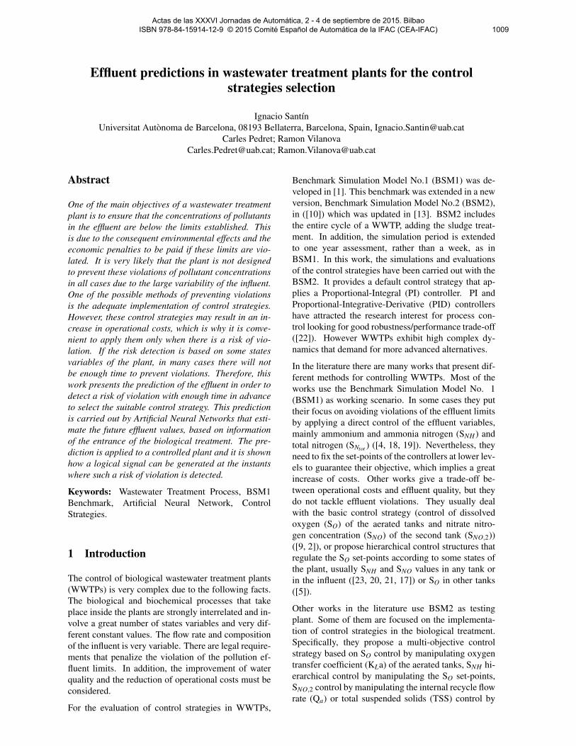
The finalized BSM2 layout (Fig. 1) includes BSM1for the biological treatment of the wastewater and thesludge treatment. A primary clarifier, a thickener forthe sludge wasted from the clarifier of biological treat-ment, a digester for treatment of the solids wastedfrom the primary clarifier and the thickened secondarysludge, as well as a dewatering unit have been alsoadded. The liquids collected in the thickening and de-watering steps are recycled ahead of the primary set-tler.

QinQbypass

Qpo QeQpo

Qw

Qa

Primaryclarifier

Activated sludge reactors

Secondaryclarifier

Thickener

Anaerobicdigester

Storagetank Dewatering

Qr

SludgeRemoval

Figure 1: BSM2 plant with notation used for flow rates

The influent dynamics are defined for 609 days bymeans of a single file, which takes into account rainfalleffect and temperature variations along the year. Fol-lowing the simulation protocol, a 200-day period ofstabilization in closed-loop using constant inputs withno noise on the measurements has to be completed be-fore using the influent file (609 days). Only data fromday 245 to day 609 are evaluated.

2.1 Activated sludge reactors

The activated sludge reactors consist in five biologi-cal reactor tanks connected in series. Qa from the lasttank complete the system. The plant is designed foran average influent dry weather flow rate of 20648.36m3/d and an average biodegradable chemical oxygendemand (COD) in the influent of 592.53 mg/l. Thetotal volume of the bioreactor is 12000 m3, 1500 m3

each anoxic tank and 3000 m3 each aerobic tank. Itshydraulic retention time, based on the average dryweather flow rate and the total tank volume, is 14hours. The internal recycle is used to supply the deni-trification step with SNO.

The Activated Sludge Model No. 1 (ASM1) [8] de-scribes the biological phenomena that take place in thebiological reactors. They define the conversion rates ofthe different variables of the biological treatment. Theproposed control strategies in this work are based onthe conversion rates of SNH (rNH ) and SNO (rNO). Theyare shown following:

rNH =−0.08ρ1 −0.08ρ2 −(

0.08+1

0.24

)ρ3 +ρ6

(1)rNO =−0.1722ρ2 +4.1667ρ3 (2)

where ρ1, ρ2, ρ3, ρ6 are four of the eight biologicalprocesses defined in ASM1. Specifically, ρ1 is the aer-obic growth of heterotrophs, ρ2 is the anoxic growthof heterotrophs, ρ3 is the aerobic growth of autotrophsand ρ6 is the ammonification of soluble organic nitro-gen. They are defined below:

ρ1 = µHT

(SS

10+SS

)(SO

0.2+SO

)XB,H (3)

where SS is the readily biodegradable substrate, XB,Hthe active heterotrophic biomass and µHT is:

µHT = 4 · exp

((Ln( 4

3

)5

)· (Tas −15)

)(4)

ρ2 = µHT

(SS

10+SS

)(0.2

0.2+SO

)(SNO

0.5+SNO

)0.8 ·XB,H

(5)

ρ3 = µAT

(SNH

1+SNH

)(SO

0.4+SO

)XB,A (6)


where Tas is the temperature, XB,A is the active au-totrophic biomass and µAT is:

µAT = 0.5 · exp

((Ln( 0.5

0.3

)5

)· (Tas −15)

)(7)

ρ6 = kaT ·SND ·XB,H (8)

where SND is the soluble biodegradable organic nitro-gen and kaT is:

kaT = 0.05 · exp

((Ln( 0.05

0.04

)5

)· (Tas −15)

)(9)

The general equations for mass balancing are as fol-lows:

• For reactor 1:

dZ1

dt=

1V1

(Qa ·Za +Qr ·Zr+

+Qpo ·Zpo + rz,1 ·V1 −Q1 ·Z1) (10)

where Z is any concentration of the process, Z1 isZ in the first reactor, Za is Z in the internal recir-culation, Zr is Z in the external recirculation, Zpois Z from the primary clarifier, V is the volume,V1 is V in the first reactor, Qpo is the overflow ofthe primary clarifier and Q1 is the flow rate in thefirst tank and it is equal to the sum of Qa, Qr andQpo.

• For reactor 2 to 5:

dZk

dt=

1Vk

(Qk−1 ·Zk−1 + rz,k ·Vk −Qk ·Zk) (11)

where k is the number of reactor and Qk is equalto Qk−1

2.2 Evaluation criteria

The performance assessment is made at two levels.The first level concerns the control. Basically, thisserves as a proof that the proposed control strategy hasbeen applied properly. The second level measures theeffect of the control strategy on plant performance. Itincludes the percentage of time that the effluent limitsare not met, the Effluent Quality Index (EQI) andthe Overall Cost Index (OCI) explained below. Theeffluent concentrations of Ntot , total COD (CODt ),SNH , TSS and Biological Oxygen Demand (BOD5)should obey the limits given in Table 1. SNtot iscalculated as the sum of SNO and Kjeldahl nitrogen(SNK j), being this the sum of organic nitrogen andSNH .

EQI is defined to evaluate the quality of the effluent.EQI is averaged over a 364 days observation periodand it is calculated weighting the different compounds

Variable ValueSNtot < 18 g N.m−3

CODt < 100 g COD.m−3

SNH < 4 g N.m−3

TSS < 30 g SS.m−3

BOD5 < 10 g BOD.m−3

Table 1: Effluent quality limits

of the effluent loads.

EQI =1

1000 ·T

t=609days∫t=245days

(2 ·T SS(t)+1 ·COD(t)+

+30 ·SNK j(t)+10 ·SNO(t)+2 ·BOD5(t)) ·Q(t) ·dt(12)

OCI is defined to evaluate the operational cost as:

OCI =AE+PE+3 ·SP+3 ·EC+ME−6 ·METprod +HEnet(13)

where AE is the aeration energy, PE is the pumpingenergy, SP is the sludge production to be disposed, ECis the consumption of external carbon source, ME isthe mixing energy, METprod is the methane productionin the anaerobic digester and HEnet is the net heatingenergy.

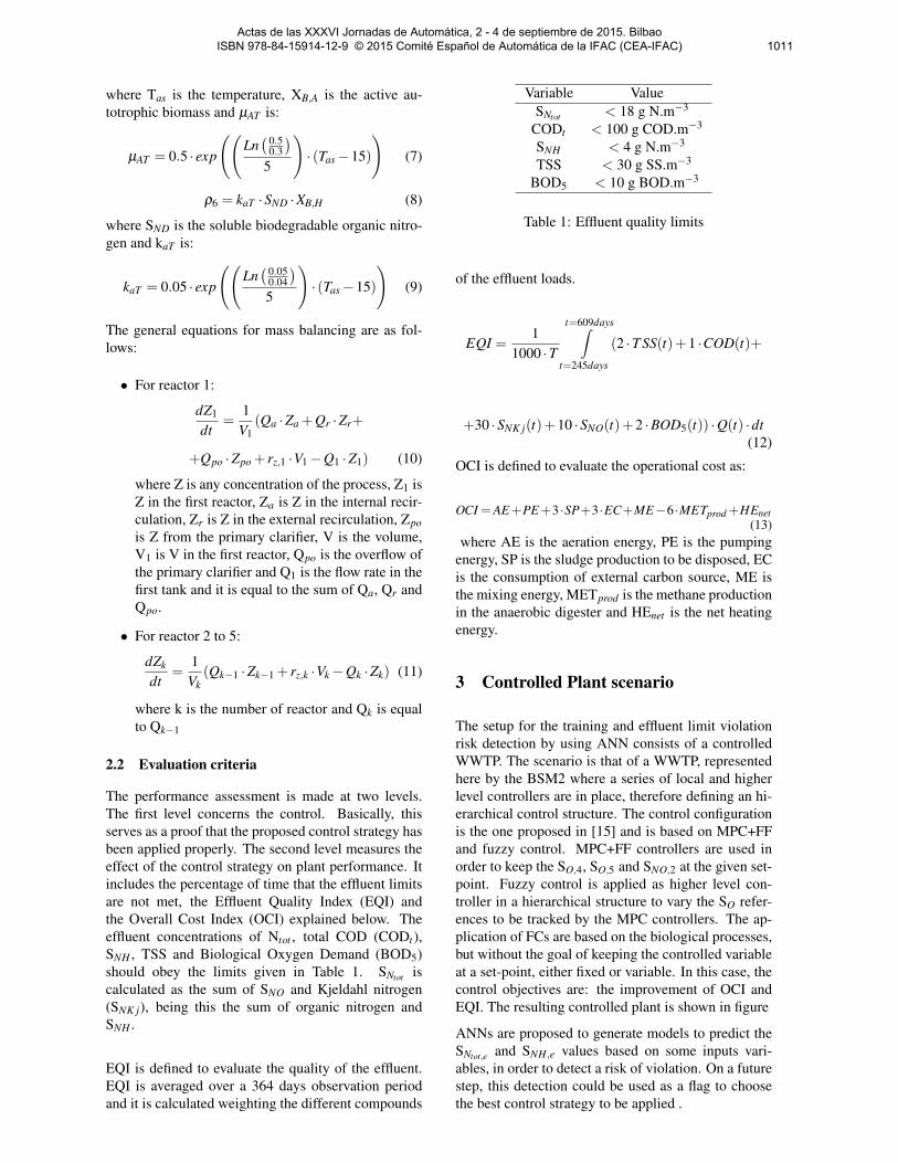
3 Controlled Plant scenario

The setup for the training and effluent limit violationrisk detection by using ANN consists of a controlledWWTP. The scenario is that of a WWTP, representedhere by the BSM2 where a series of local and higherlevel controllers are in place, therefore defining an hi-erarchical control structure. The control configurationis the one proposed in [15] and is based on MPC+FFand fuzzy control. MPC+FF controllers are used inorder to keep the SO,4, SO,5 and SNO,2 at the given set-point. Fuzzy control is applied as higher level con-troller in a hierarchical structure to vary the SO refer-ences to be tracked by the MPC controllers. The ap-plication of FCs are based on the biological processes,but without the goal of keeping the controlled variableat a set-point, either fixed or variable. In this case, thecontrol objectives are: the improvement of OCI andEQI. The resulting controlled plant is shown in figure

ANNs are proposed to generate models to predict theSNtot,e and SNH,e values based on some inputs vari-ables, in order to detect a risk of violation. On a futurestep, this detection could be used as a flag to choosethe best control strategy to be applied .


Qpo

MPC+FF

SO,4

KLa,5KLa,4KLa,3

SO,4set-point

SO,5set-point

SO,5

Fuzzy

SNH,5

MPC+FF

MPC+FFSNO,2set-point(1 mg/l)

SNO,2

Figure 2: BSM2 Hierarchical control for ANN train-ing and risk prediction

4 Artificial Neural Network

ANNs are inspired by the structure and function ofnervous systems, where the neuron is the fundamen-tal element ([25]). ANNs are composed of sim-ple elements, called neurons, operating in parallel.ANNs have proved to be effective for many complexfunctions, as pattern recognition, system identifica-tion, classification, speech vision, and control systems([24, 14]). ANNs are frequently used for nonlinearsystem identification, to model complex relationshipsbetween the inputs and the outputs of a system, as it isthe case of WWTPs.

An artificial neuron is a device that generates a singleoutput y from a set of inputs xi (i = 1 ... n). Thisartificial neuron consists of the following elements:

• Set of xi inputs with n components

• Set of weights wi j that represent the interactionbetween the neuron j and neuron i.

• Propagation rule, a weighted sum of the scalarproduct of the input vector and the weight vector:hi(t) = ∑wi j · x j.

• Activation function provides the state of the neu-ron based on of the previous state and the propa-gation rule (i.e. threshold, piecewise linear, sig-moid, Gaussian): ai(t) = f (ai(t −1),hi(t)) :.

• The output y(t) that depends on the activationstate.

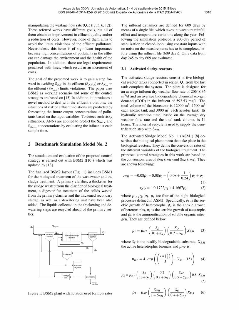
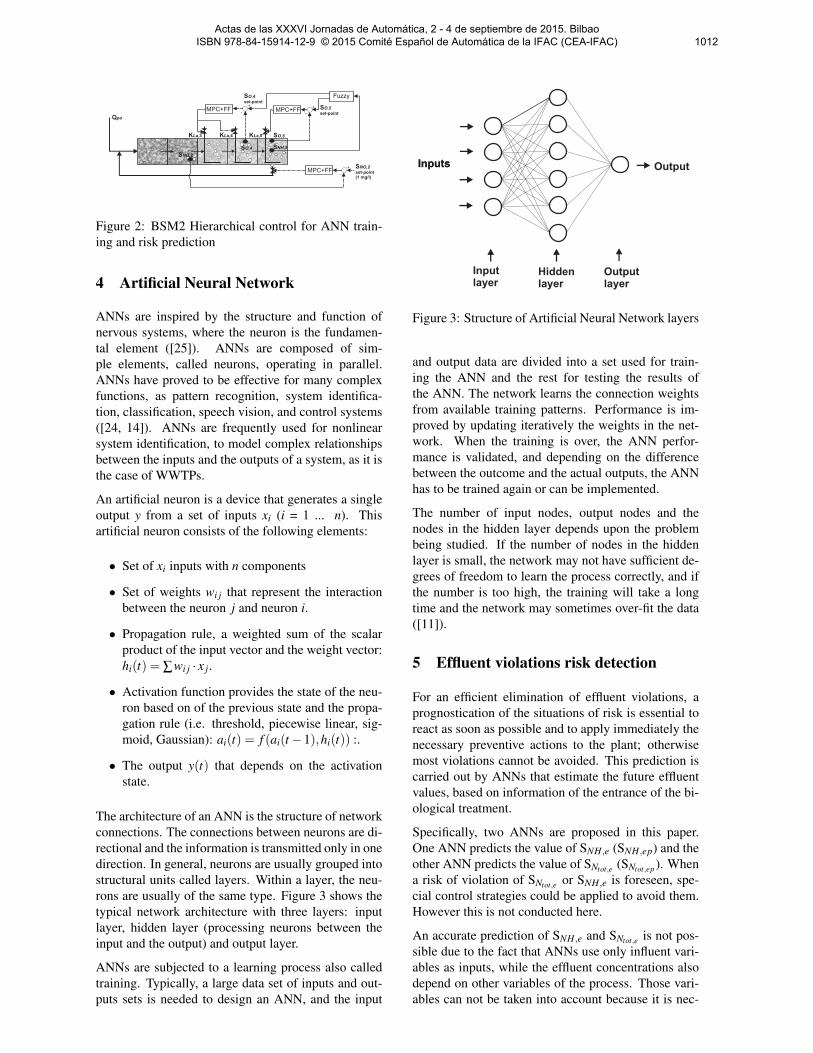
The architecture of an ANN is the structure of networkconnections. The connections between neurons are di-rectional and the information is transmitted only in onedirection. In general, neurons are usually grouped intostructural units called layers. Within a layer, the neu-rons are usually of the same type. Figure 3 shows thetypical network architecture with three layers: inputlayer, hidden layer (processing neurons between theinput and the output) and output layer.

ANNs are subjected to a learning process also calledtraining. Typically, a large data set of inputs and out-puts sets is needed to design an ANN, and the input

Inputs OutputInputs

Inputlayer

Outputlayer

Hiddenlayer

Figure 3: Structure of Artificial Neural Network layers

and output data are divided into a set used for train-ing the ANN and the rest for testing the results ofthe ANN. The network learns the connection weightsfrom available training patterns. Performance is im-proved by updating iteratively the weights in the net-work. When the training is over, the ANN perfor-mance is validated, and depending on the differencebetween the outcome and the actual outputs, the ANNhas to be trained again or can be implemented.

The number of input nodes, output nodes and thenodes in the hidden layer depends upon the problembeing studied. If the number of nodes in the hiddenlayer is small, the network may not have sufficient de-grees of freedom to learn the process correctly, and ifthe number is too high, the training will take a longtime and the network may sometimes over-fit the data([11]).

5 Effluent violations risk detection

For an efficient elimination of effluent violations, aprognostication of the situations of risk is essential toreact as soon as possible and to apply immediately thenecessary preventive actions to the plant; otherwisemost violations cannot be avoided. This prediction iscarried out by ANNs that estimate the future effluentvalues, based on information of the entrance of the bi-ological treatment.

Specifically, two ANNs are proposed in this paper.One ANN predicts the value of SNH,e (SNH,ep) and theother ANN predicts the value of SNtot,e (SNtot,ep ). Whena risk of violation of SNtot,e or SNH,e is foreseen, spe-cial control strategies could be applied to avoid them.However this is not conducted here.

An accurate prediction of SNH,e and SNtot,e is not pos-sible due to the fact that ANNs use only influent vari-ables as inputs, while the effluent concentrations alsodepend on other variables of the process. Those vari-ables can not be taken into account because it is nec-


essary to predict the risk of effluent violations withenough time in advance. Moreover, all data used topredict the risk has to be easily measurable. However,as we will see, with an adequate choice of the inputvariables of ANNs, it is possible to achieve an ade-quate approximation in order to detect a risk of viola-tion for applying the suitable control strategy.

Therefore, the inputs of ANNs have been determinedaccording to the mass balance equations (10 and 11)explained in Section 2.1. The variables used to per-form the prediction for both ANNs are Qpo, Zpo andTas. The variable Qa has also been used as an input forthe ANN that predicts SNtot,e , but it is not used to pre-dict SNH,e because it is a manipulated variable in thecontrol strategy applied to remove SNH,e violations.Specifically, SNH from the primary clarifier (SNH,po)is the pollutant concentration chosen as a predictor forboth ANNs. On one hand, SNH and SNO are the pollu-tants with higher influence in SNtot,e , but SNO,po is verylow and it is not taken in account. On the other hand,SNH,po not only affects largely SNH,e, but also affectsthe nitrification process, the consequent SNO produc-tion and therefore the resulting SNtot,e .

Tas is also added as a predictor variable due to its in-fluence in the nitrification and denitrification processes(5 and 6). SNH,e and SNtot,e values are inversely propor-tional to the Tas values.

Finally, due to the mentioned reasons, the inputs forthe ANNs are:

• Inputs of ANN for SNH,e model prediction: Qpo,SNH,po, Qpo · SNH,po, Tas.

• Inputs of ANN for SNtot,e model prediction: Qpo,SNH,po, Qpo · SNH,po, Tas, Qa.

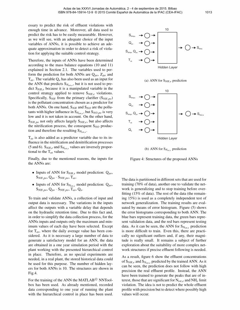
To train and validate ANNs, a collection of input andoutput data is necessary. The variations in the inputsaffect the outputs with a variable delay that dependson the hydraulic retention time. Due to this fact and,in order to simplify the data collection process, for theANNs inputs and outputs only the maximum and min-imum values of each day have been selected. Exceptfor Tas, where the daily average value has been con-sidered. As it is necessary a large number of data togenerate a satisfactory model for an ANN, the dataare obtained in a one year simulation period with theplant working with the presented hierarchical controlin place. Therefore, as no special experiments areneeded, in a real plant, the stored historical data couldbe used for this purpose. The number of hidden lay-ers for both ANNs is 10. The structures are shown inFig.4.

For the training of the ANN the MATLAB c© NNTool-box has been used. As already mentioned, recordeddata corresponding to one year of running the plantwith the hierarchical control in place has been used.

SNHpo

Qpo

S QNHpo po

Tas

SNHe

10

Hidden Layer

(a) ANN for SNH,e prediction

SNHpo

Qpo

S QNHpo po

Tas

SNtot,e

10

Hidden Layer

Qa

(b) ANN for SNtot,e prediction

Figure 4: Structures of the proposed ANNs

The data is partitioned in different sets that are used fortraining (70% of data), another one to validate the net-work is generalizing and to stop training before over-fitting (15% of data). The rest of the data (the remain-ing 15%) is used as a completely independent test ofnetwork generalization. The training results are eval-uated by means of error histogram. Figure (5) showsthe error histograms corresponding to both ANN. Theblue bars represent training data, the green bars repre-sent validation data, and the red bars represent testingdata. As it can be seen, the ANN for SNtot,e predictionis more difficult to train. Even this, there are practi-cally no significant outliers and, if any, their magni-tude is really small. It remains a subject of furtherexploration about the suitability of more complex net-work structures if precise effluent following is needed.

As a result, figure 6 show the effluent concentrationsof SNH,e and SNtot,e predicted by the trained ANN. As itcan be seen, the prediction does not follow with highprecision the real effluent profile. Instead, the ANNhave been trained to generate the peaks that are of in-terest, those that are significant for Ntot,e and NHe limitviolation. The idea is not to predict the whole effluentprofile with precision but to detect where possibly highvalues will occur.


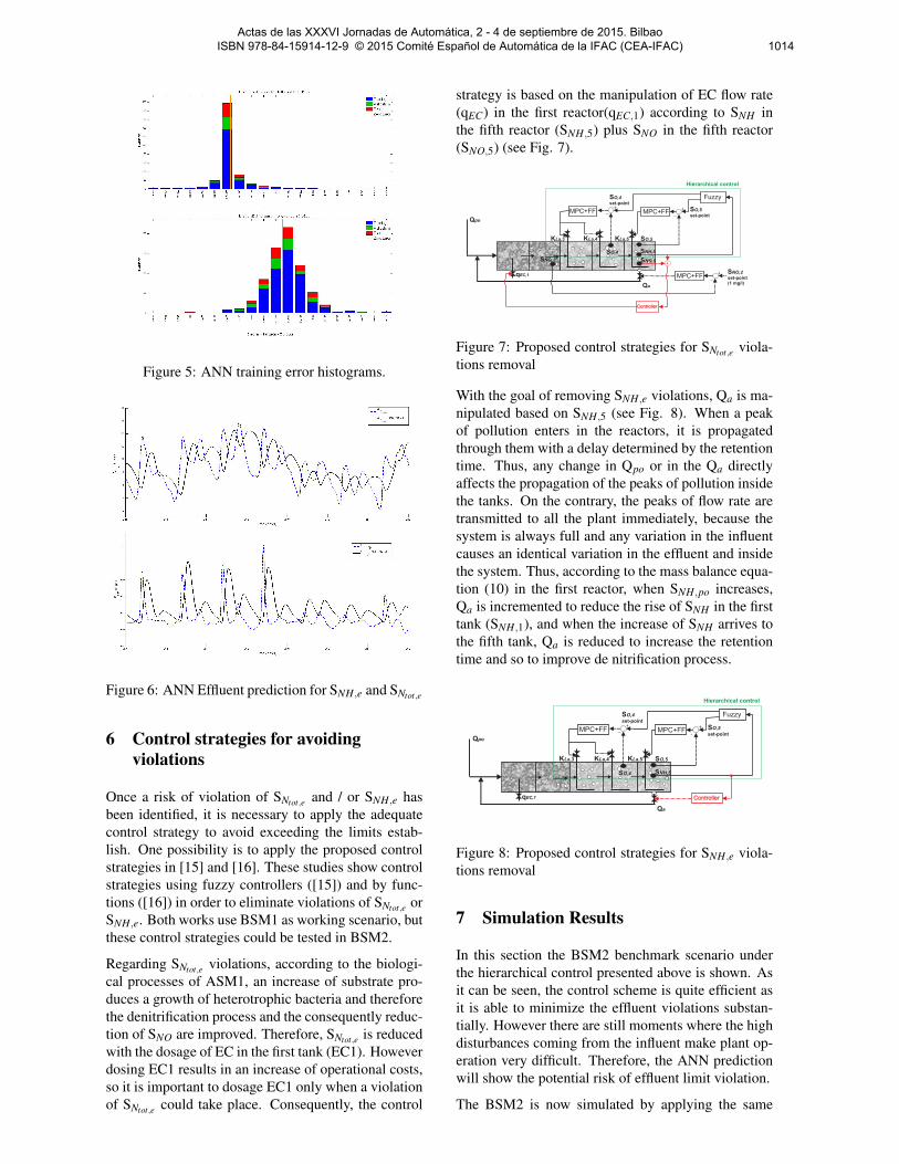
Figure 5: ANN training error histograms.

Figure 6: ANN Effluent prediction for SNH,e and SNtot,e

6 Control strategies for avoidingviolations

Once a risk of violation of SNtot,e and / or SNH,e hasbeen identified, it is necessary to apply the adequatecontrol strategy to avoid exceeding the limits estab-lish. One possibility is to apply the proposed controlstrategies in [15] and [16]. These studies show controlstrategies using fuzzy controllers ([15]) and by func-tions ([16]) in order to eliminate violations of SNtot,e orSNH,e. Both works use BSM1 as working scenario, butthese control strategies could be tested in BSM2.

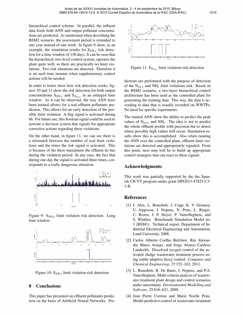
Regarding SNtot,e violations, according to the biologi-cal processes of ASM1, an increase of substrate pro-duces a growth of heterotrophic bacteria and thereforethe denitrification process and the consequently reduc-tion of SNO are improved. Therefore, SNtot,e is reducedwith the dosage of EC in the first tank (EC1). Howeverdosing EC1 results in an increase of operational costs,so it is important to dosage EC1 only when a violationof SNtot,e could take place. Consequently, the control

strategy is based on the manipulation of EC flow rate(qEC) in the first reactor(qEC,1) according to SNH inthe fifth reactor (SNH,5) plus SNO in the fifth reactor(SNO,5) (see Fig. 7).

Qpo

Qa

MPC+FF

SO,4

KLa,5KLa,4KLa,3

SO,4set-point

SO,5set-point

SO,5

Fuzzy

SNH,5

MPC+FF

MPC+FFSNO,2set-point(1 mg/l)

SNO,2

qEC,1

Controller

SNO,5

Hierarchical control

Figure 7: Proposed control strategies for SNtot,e viola-tions removal

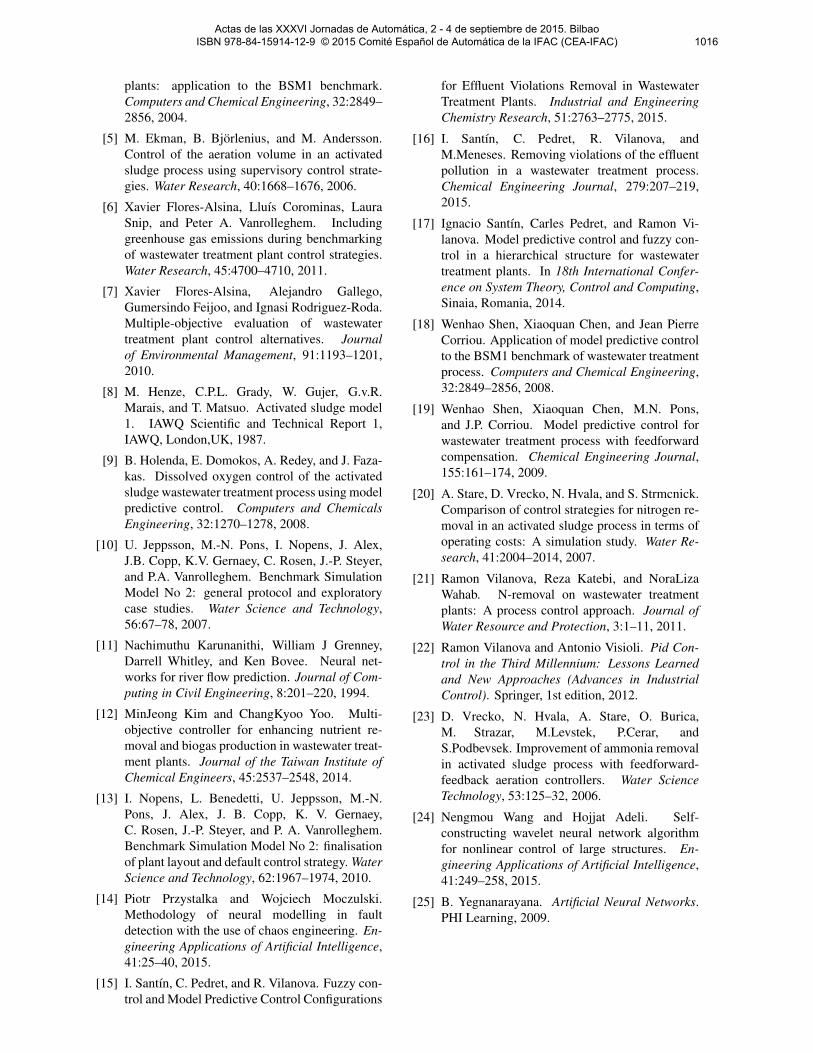
With the goal of removing SNH,e violations, Qa is ma-nipulated based on SNH,5 (see Fig. 8). When a peakof pollution enters in the reactors, it is propagatedthrough them with a delay determined by the retentiontime. Thus, any change in Qpo or in the Qa directlyaffects the propagation of the peaks of pollution insidethe tanks. On the contrary, the peaks of flow rate aretransmitted to all the plant immediately, because thesystem is always full and any variation in the influentcauses an identical variation in the effluent and insidethe system. Thus, according to the mass balance equa-tion (10) in the first reactor, when SNH,po increases,Qa is incremented to reduce the rise of SNH in the firsttank (SNH,1), and when the increase of SNH arrives tothe fifth tank, Qa is reduced to increase the retentiontime and so to improve de nitrification process.

Qpo

Qa

MPC+FF

SO,4

KLa,5KLa,4KLa,3

SO,4set-point

SO,5set-point

SO,5

Fuzzy

SNH,5

MPC+FF

ControllerqEC,1

Hierarchical control

Figure 8: Proposed control strategies for SNH,e viola-tions removal

7 Simulation Results

In this section the BSM2 benchmark scenario underthe hierarchical control presented above is shown. Asit can be seen, the control scheme is quite efficient asit is able to minimize the effluent violations substan-tially. However there are still moments where the highdisturbances coming from the influent make plant op-eration very difficult. Therefore, the ANN predictionwill show the potential risk of effluent limit violation.

The BSM2 is now simulated by applying the same


hierarchical control scheme. In parallel, the influentdata feeds both ANN and output pollutant concentra-tions are predicted. As mentioned when describing theBSM2 scenario, the assessment period is extended toone year instead of one week. In figure 9 show, as anexample, the simulation results for SNH,e risk detec-tion for a time window of 150 days. It can be seen thatthe hierarchical, two-level control system, operates theplant quite well, so there are practically no limit vio-lations. Two risk situations are detected. Therefore itis on such time instants when supplementary controlactions will be needed.

In order to better show how risk detection works, fig-ures 10 and 11 show the risk detection for both outputconcentrations SNH,e and SNtot,e in an enlarged timewindow. As it can be observed, the way ANN havebeen trained allows for a real effluent pollutants pre-diction. This allows for an early detection of the pos-sible limit violation. A flag signal is activated during6h. For future use, this boolean signal could be used toactivate a decision system that signals for appropriatecorrective actions regarding these violations.

On the other hand, in figure 11, we can see there isa mismatch between the number of real limit viola-tions and the times the risk signal is activated. Thisis because of the three maximums the effluent do hasduring the violation period. In any case, the fact thatduring one day the signal is activated three times, cor-responds to a really dangerous sittuation.

Figure 9: SNH,e limit violation risk detection. Longtime window.

Figure 10: SNH,e limit violation risk detection

8 Conclusions

This paper has presented an effluent pollutants predic-tion on the basis of Artificial Neural Networks. Pre-

Figure 11: SNtot,e limit violation risk detection

dictions are performed with the purpose of detectionof the Ntot,e and NHe limit violations risk. Based onthe BSM2 scenario, a two-layer hierarchical controlarchitecture has been used as the controlled plant forgenerating the training data. This way, the data is ac-cording to data that is usually recorded on WWTPs.No need for specific experiments.

The trained ANN show the ability to predict the peakvalues of Ntot,e and NHe. The idea is not to predictthe whole effluent profile with precision but to detectwhere possibly high values will occur. Simulation re-sults show this is accomplished. Also when runningthe ANN over the controlled plant, effluent limit vio-lations are detected and appropriately signaled. Fromthis point, next step will be to build up appropriatecontrol strategies that can react to these signals.

Acknowledgments

This work was partially supported by the the Span-ish CICYT program under grant DPI2013-47825-C3-1-R.

References[1] J. Alex, L. Benedetti, J. Copp, K. V. Gernaey,

U. Jeppsson, I. Nopens, N. Pons, L. Rieger,C. Rosen, J. P. Steyer, P. Vanrolleghem, andS. Winkler. Benchmark Simulation Model no.1 (BSM1). Technical report, Department of In-dustrial Electrical Engineering and Automation,Lund University, 2008.

[2] Carlos Alberto Coelho Belchior, Rui Alexan-dre Matos Araujo, and Jorge Afonso CardosoLandeckb. Dissolved oxygen control of the ac-tivated sludge wastewater treatment process us-ing stable adaptive fuzzy control. Computer andChemical Engineering, 37:152–162, 2011.

[3] L. Benedetti, B. De Baets, I. Nopens, and P.A.Vanrolleghem. Multi-criteria analysis of wastew-ater treatment plant design and control scenariosunder uncertainty. Environmental Modelling andSoftware, 25:616–621, 2009.

[4] Jean Pierre Corriou and Marie Noelle Pons.Model predictive control of wastewater treatment


plants: application to the BSM1 benchmark.Computers and Chemical Engineering, 32:2849–2856, 2004.

[5] M. Ekman, B. Bjorlenius, and M. Andersson.Control of the aeration volume in an activatedsludge process using supervisory control strate-gies. Water Research, 40:1668–1676, 2006.

[6] Xavier Flores-Alsina, Lluıs Corominas, LauraSnip, and Peter A. Vanrolleghem. Includinggreenhouse gas emissions during benchmarkingof wastewater treatment plant control strategies.Water Research, 45:4700–4710, 2011.

[7] Xavier Flores-Alsina, Alejandro Gallego,Gumersindo Feijoo, and Ignasi Rodriguez-Roda.Multiple-objective evaluation of wastewatertreatment plant control alternatives. Journalof Environmental Management, 91:1193–1201,2010.

[8] M. Henze, C.P.L. Grady, W. Gujer, G.v.R.Marais, and T. Matsuo. Activated sludge model1. IAWQ Scientific and Technical Report 1,IAWQ, London,UK, 1987.

[9] B. Holenda, E. Domokos, A. Redey, and J. Faza-kas. Dissolved oxygen control of the activatedsludge wastewater treatment process using modelpredictive control. Computers and ChemicalsEngineering, 32:1270–1278, 2008.

[10] U. Jeppsson, M.-N. Pons, I. Nopens, J. Alex,J.B. Copp, K.V. Gernaey, C. Rosen, J.-P. Steyer,and P.A. Vanrolleghem. Benchmark SimulationModel No 2: general protocol and exploratorycase studies. Water Science and Technology,56:67–78, 2007.

[11] Nachimuthu Karunanithi, William J Grenney,Darrell Whitley, and Ken Bovee. Neural net-works for river flow prediction. Journal of Com-puting in Civil Engineering, 8:201–220, 1994.

[12] MinJeong Kim and ChangKyoo Yoo. Multi-objective controller for enhancing nutrient re-moval and biogas production in wastewater treat-ment plants. Journal of the Taiwan Institute ofChemical Engineers, 45:2537–2548, 2014.

[13] I. Nopens, L. Benedetti, U. Jeppsson, M.-N.Pons, J. Alex, J. B. Copp, K. V. Gernaey,C. Rosen, J.-P. Steyer, and P. A. Vanrolleghem.Benchmark Simulation Model No 2: finalisationof plant layout and default control strategy. WaterScience and Technology, 62:1967–1974, 2010.

[14] Piotr Przystalka and Wojciech Moczulski.Methodology of neural modelling in faultdetection with the use of chaos engineering. En-gineering Applications of Artificial Intelligence,41:25–40, 2015.

[15] I. Santın, C. Pedret, and R. Vilanova. Fuzzy con-trol and Model Predictive Control Configurations

for Effluent Violations Removal in WastewaterTreatment Plants. Industrial and EngineeringChemistry Research, 51:2763–2775, 2015.

[16] I. Santın, C. Pedret, R. Vilanova, andM.Meneses. Removing violations of the effluentpollution in a wastewater treatment process.Chemical Engineering Journal, 279:207–219,2015.

[17] Ignacio Santın, Carles Pedret, and Ramon Vi-lanova. Model predictive control and fuzzy con-trol in a hierarchical structure for wastewatertreatment plants. In 18th International Confer-ence on System Theory, Control and Computing,Sinaia, Romania, 2014.

[18] Wenhao Shen, Xiaoquan Chen, and Jean PierreCorriou. Application of model predictive controlto the BSM1 benchmark of wastewater treatmentprocess. Computers and Chemical Engineering,32:2849–2856, 2008.

[19] Wenhao Shen, Xiaoquan Chen, M.N. Pons,and J.P. Corriou. Model predictive control forwastewater treatment process with feedforwardcompensation. Chemical Engineering Journal,155:161–174, 2009.

[20] A. Stare, D. Vrecko, N. Hvala, and S. Strmcnick.Comparison of control strategies for nitrogen re-moval in an activated sludge process in terms ofoperating costs: A simulation study. Water Re-search, 41:2004–2014, 2007.

[21] Ramon Vilanova, Reza Katebi, and NoraLizaWahab. N-removal on wastewater treatmentplants: A process control approach. Journal ofWater Resource and Protection, 3:1–11, 2011.

[22] Ramon Vilanova and Antonio Visioli. Pid Con-trol in the Third Millennium: Lessons Learnedand New Approaches (Advances in IndustrialControl). Springer, 1st edition, 2012.

[23] D. Vrecko, N. Hvala, A. Stare, O. Burica,M. Strazar, M.Levstek, P.Cerar, andS.Podbevsek. Improvement of ammonia removalin activated sludge process with feedforward-feedback aeration controllers. Water ScienceTechnology, 53:125–32, 2006.

[24] Nengmou Wang and Hojjat Adeli. Self-constructing wavelet neural network algorithmfor nonlinear control of large structures. En-gineering Applications of Artificial Intelligence,41:249–258, 2015.

[25] B. Yegnanarayana. Artificial Neural Networks.PHI Learning, 2009.


efﬂuent predictions in wastewater treatment plants for the

Documents