Eigenvector Centrality: Illustrations Supporting the

Utility of Extracting More Than One Eigenvector to

Obtain Additional Insights into Networks and

Interdependent Structures

Dawn Iacobuccia, Rebecca McBrideb, and Deidre L.

Popovichc

Abstract

Among the many centrality indices used to detect structures of actors’ positions in networks is the

use of the first eigenvector of an adjacency matrix that captures the connections among the actors.

This research considers the seeming pervasive current practice of using only the first eigenvector.

It is shows that, as in other statistical applications of eigenvectors, subsequent vectors can also

contain illuminating information. Several small examples, and Freeman’s EIES network, are used

to illustrate that while the first eigenvector is certainly informative, the second (and subsequent)

eigenvector(s) can also be equally tractable and informative.

Keywords: centrality, eigenvector centrality, social networks

_____________________________

a Corresponding author: Vanderbilt University, Owen Graduate School of Management, 401 21st

Avenue South, Nashville, TN, 32703, U.S.A., dawn.iacobucci@owen.vanderbilt.edu

b Calvin College, Department of Political Science, DeVos Communication Center 261G, Grand

Rapids, MI, 49546-4301, U.S.A., ram38@calvin.edu.

c Department of Marketing, Rawls College of Business, Texas Tech University, Lubbock, TX,

79409, U.S.A., deidre.popovich@ttu.edu.

1

Scholars who study social networks often begin with an analysis to determine which actors are the

most important, or the most central to a network. For example, in an office environment, to

understand a network of colleagues, it would be important to identify the most important players

in that office environment. A challenge in social network analysis comes in trying to figure out the

best way to understand importance or centrality. It could be that the actors with the largest number

of ties are the most important (as reflected by degree centrality), for example the colleague who

has meetings with the largest number of other colleagues, yet presumably quantity does not equal

quality, and frequent meetings can be a waste of time. On the other hand, it could be that the

colleagues who seem to be the link between other colleagues are important or powerful, given that

their connections imply a means of access among others in the network (reflected by betweenness

centrality). However, neither of these measures would take into account the simple fact that there

is more power in being connected to powerful people than there is in being connected to a lot of

people with limited access or resources. Eigenvector centrality is a centrality index that calculates

the centrality of an actor based not only on their connections, but also based on the centrality of

that actor’s connections.

Thus, eigenvector centrality can be important, and furthermore, social networks and their study

are more popular than ever. Eigenvector centralities have become a staple centrality index, along

with degree, closeness, and betweenness (recall: degrees reflect volumes and strengths of ties,

closeness captures the extent to which relations traverse few “degrees of separation,” and

betweenness highlights actors who connect sections of the network; Freeman, 1979). All four

centrality indices are included in social network texts (cf., Knoke and Yang, 2007; Scott, 2012;

Wasserman and Faust, 1994), and in research articles that compare the performance of centrality

indices (cf. Borgatti 2005; Borgatti, Carley, and Krackhardt, 2006; Costenbader and Valente, 2003;

Friedkin, 1991; Rothenberg et al., 1995; Smith and Moody, 2013; Stephenson and Zelen, 1989),

as well as in the major social network analysis software packages (cf., UCINet, Pajek, NetMiner,

NetworkX and LibSNA, NodeXL and SNAP, even Mathematica and StatNet).

When using eigenvector-based centrality, early definitions and current practice are focused on the

first eigenvector of the sociomatrix that contains the ties among the actors. The reasoning is sound

in that the first eigenvector is associated with the largest eigenvalue, thus capturing the majority

of the variance contained in the network. However, there often remains further information about

the network structure that subsequent eigenvectors can explain. For example, where the first

eigenvector is likely to reflect volumes and strengths of connections among the actors, a second or

third eigenvector can delineate those in separate groups within the network who behave in

somewhat equivalent manners, or other elements of network structure that can be informative in

understanding the actors and the patterns that link them. The research in this paper is conducted to

demonstrate that the extraction of only the first eigenvector can be, and in even modest-sized

networks typically will be, insufficient for a more comprehensive understanding of the network.

This research is not intended to produce a new centrality measure; rather to evaluate the status of

the eigenvector centrality, and suggest that extending it beyond the extraction of only the first

eigenvector can be insightful, as illustrated with several examples. To this end, this paper

demonstrates that network scholars who consider additional eigenvectors (second, third, and

subsequent) will typically be rewarded in obtaining richer insights about additional aspects of

network interdependencies. Even that recommendation might not be said to cover “new ground”

2

in that early social network scholars (e.g., Comrey, 1962) seem to have been more willing to

consider multiple eigenvectors, such as research modeling networks of “consensus analysis” in

anthropology (e.g., Romney, Weller, and Batchelder, 1986; see also Kumbasar, 1996). However,

more recent practice has slipped back toward a simpler reduction of deriving only a single

eigenvector, and to not consider the greater vector portfolio would seem to be a lost opportunity.

A reviewer also noted that this issue may be all the more relevant in today’s scholarship, given the

relevance of eigenvector, or eigenvector-like structures, in different models and domains. For

example, much of “community detection” regularly relies upon singular values (recall these are

like eigenvectors, but drawn from asymmetric matrices; Wang and Sukthankar, 2015). In addition,

most latent space models are ultimately based on eigenvector-like structures, including some of

the recent work on exponential random graphs (cf., Hoff, Raftery, and Handcock, 2002; Hoff and

Ward, 2004).

The remainder of this paper is organized as follows:

1. Eigenvector centrality is reviewed—its conceptual and mathematical definition.

2. Several simple networks are used to illustrate that a single eigenvector may indeed suffice

to characterize the network, but that with very little additional complications in structure,

very often driven by sheer size, a second or third eigenvector (or more) will be helpful and

informative in describing additional aspects of the actors’ positions in a network.

3. The eigenvectors are then analyzed for a known, real social network, the electronic

exchanges in the EIES Freeman data (Freeman and Freeman, 1979). It is shown that the

first eigenvector is correlated with (i.e., somewhat redundant with) other standard measures

of centrality, and the second eigenvector illuminates other structural properties in the

network that are shown to be related to information on the actors’ attributes.

The paper concludes by suggesting that network scholars may wish to modify how they proceed

with eigenvector centralities, treating them more analogously to traditional uses of eigenvalues

and eigenvectors, such as in principal components, namely by extracting multiple vectors.

Eigenvectors—Basics and Centrality

Before turning to eigenvector centralities eigenvectors are first briefly reviewed. The essence of

the questions underlying eigenvector-based analyses share the quest for data reduction, from some

number of raw variables to a smaller set of vectors, such as principal components or factors, that

somehow capture or approximate reasonably well the variability or information in the raw data.

Sometimes a single vector will suffice, but frequently more eigenvectors are needed, and one

central question in principal components and factor analysis is: How many components or factors

to extract?

More precisely, eigenvalues and eigenvectors form the basis of multivariate statistical models,

such as principal components and factor analysis (e.g., Kim and Mueller, 1978; Manly, 1986; see

Appendix A). In those models, researchers pose the question as to whether a set of p variables

might share sufficient covariability to be described by a single, underlying principal component or

factor. For example, it might be the case that a person’s subjective ratings of his or her “perceived

health” and “mobility” may be both adequately described by age (or perceived age), with the

concept (or “factor”) of age serving as the underlying principle construct,, meaning knowledge of

the person’s age would be sufficient for estimations of the person’s likely standings on perceived

health and mobility.

3

The mechanics of the model are familiar: a dataset X that is N (sample size) by p (number of

variables) is processed into a p×p correlation matrix, R. The correlation matrix is factored into two

unique matrices: one of eigenvalues 𝚲 (ordered 𝜆1 ≥ 𝜆2 ≥ ⋯ ≥ 𝜆𝑝), one of eigenvectors 𝑽 (each

column with entries 𝑣1, 𝑣2, … 𝑣𝑝 ), and its transpose 𝑽′ , 𝑹 = 𝑽𝚲𝑽′ , such that 𝑦𝑖 = 𝑣1𝑋𝑖1 +

𝑣2𝑋𝑖2 + ⋯ + 𝑣𝑝𝑋𝑖𝑝 (Seber, 1984).

The first eigenvector (column of V) contains the weights that will optimally transform the original

p variables (e.g., health and mobility) into a single new score (e.g., a scale of perceived age) that

explains the maximum possible variance in the data matrix X (that variance being 𝜆). The first

eigenvector yields weights for each variable. If the weight coefficients are high for health and

mobility, then instead of working with both health and mobility as separate variables in subsequent

analyses, it should be acceptable to use the perceived age scale instead (i.e. doing so would be

sufficient in explaining the health and mobility data, and it may be optimal in terms of parsimony

to use one rather than two variables, per this example). Subsequent eigenvectors 2, 3, …, p will

contain weights that create new variables that explain the maximum amount of remaining variance

(such as smoking history, which would not be explained by health, mobility, or age) subject to the

constraint that each newly created variable is uncorrelated (not redundant) with the previous

composite variables (Tabachnick and Fidell, 2006).

The application of eigen-models is not typically limited to the extraction of only the first

eigenvector (Kim and Mueller, 1978; Seber, 1984). In principal components, the frequently

employed heuristic is to extract as many eigenvectors as there exist eigenvalues that exceed 1.0.

The reasoning is that given that the eigenvalue is the variance of the composite score formed using

the weights in the eigenvector, the new composite score should explain at least as much variance

as that in a single variable, which is 1.0 as expressed in standardized form, such as in a correlation

matrix (Manly, 1986). In factor analysis, the eigenvalues are examined for their relative size, and

the number of factors is determined to be that which corresponds to the number of relatively large

eigenvalues (Tabachnick and Fidell, 2006).1 A sociomatrix is not a correlation or covariance

matrix, so the rule of thumb to extract as many eigenvectors as there are eigenvalues that exceed

1.0 (as the new composite variable’s unit variance as in principal components analysis) is not

directly applicable. Instead, the judgment of the relative size of the ordered eigenvalues (as in

factor analysis) is the rule of thumb that transfers more readily in the application to social networks.

And of course, it would be prudent to not extract eigenvectors associated with eigenvalues that are

zero or negative.

In sum, many research articles in the social and physical sciences find it useful to extract more

than one eigenvector—the amount and patterns of variability in the source data warrant doing so.

Some data may certainly be analyzed and captured sufficiently with a single component or factor,

but it seems that many more papers report multiple components or factors due to the complexities

of the data and the research questions at hand.

1 Note that these analyses are obviously conducted on square, symmetric correlation matrices. When an eigenvector

model is used on a square, symmetric sociomatrix, it will operate similarly. If the sociomatrix is not symmetric, or if

it is two-mode, a singular value decomposition yields analogous information (Namboodiri, 1984; Seber, 1984).

4

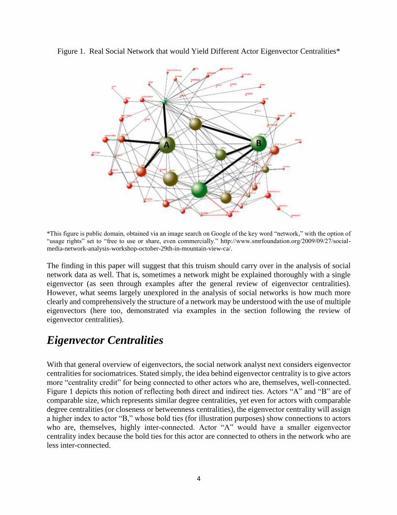
Figure 1. Real Social Network that would Yield Different Actor Eigenvector Centralities*

*This figure is public domain, obtained via an image search on Google of the key word “network,” with the option of

“usage rights” set to “free to use or share, even commercially.” http://www.smrfoundation.org/2009/09/27/social-

media-network-analysis-workshop-october-29th-in-mountain-view-ca/.

The finding in this paper will suggest that this truism should carry over in the analysis of social

network data as well. That is, sometimes a network might be explained thoroughly with a single

eigenvector (as seen through examples after the general review of eigenvector centralities).

However, what seems largely unexplored in the analysis of social networks is how much more

clearly and comprehensively the structure of a network may be understood with the use of multiple

eigenvectors (here too, demonstrated via examples in the section following the review of

eigenvector centralities).

Eigenvector Centralities

With that general overview of eigenvectors, the social network analyst next considers eigenvector

centralities for sociomatrices. Stated simply, the idea behind eigenvector centrality is to give actors

more “centrality credit” for being connected to other actors who are, themselves, well-connected.

Figure 1 depicts this notion of reflecting both direct and indirect ties. Actors “A” and “B” are of

comparable size, which represents similar degree centralities, yet even for actors with comparable

degree centralities (or closeness or betweenness centralities), the eigenvector centrality will assign

a higher index to actor “B,” whose bold ties (for illustration purposes) show connections to actors

who are, themselves, highly inter-connected. Actor “A” would have a smaller eigenvector

centrality index because the bold ties for this actor are connected to others in the network who are

less inter-connected.

5

To capture such patterns of direct and indirect connections, Bonacich (1972) built on Katz (1953)

and proposed that the (first) eigenvector (corresponding to the largest eigenvalue) of an adjacency

matrix could serve as such a centrality measure. Bonacich’s (1972) idea was that the eigenvectors

(of symmetric sociomatrices, and singular value decompositions of asymmetric sociomatrices)

would reflect different weighting of ties to partners who, themselves, are highly central versus

partners who are less central. Analogous to the example of correlations of survey items, first

eigenvectors frequently reflect actors’ overall volumes of ties, and it will be demonstrated that

second and subsequent eigenvectors reflect other differentiating patterns of the ties.

More precisely, for a 𝑔 × 𝑔 sociomatrix or adjacency matrix on 𝑔 actors, denoted 𝑿 = {𝑥𝑖𝑗}, for

actors in rows 𝑖 = 1,2, … 𝑔 extending ties to the same set of actors in columns 𝑗 = 1,2, … 𝑔, the

eigenvector, v (and eigenvalue, 𝜆 ), are obtained from the familiar equation: 𝑿𝒗 = 𝜆𝒗. The

eigenvector score for actor 𝑖 is 𝐶𝐸𝑉(𝑖), a weighted function of the statuses of the other actors to

whom actor 𝑖 is connected: 𝐶𝐸𝑉(𝑖) = 𝑥1𝑖𝑣1 + 𝑥2𝑖𝑣2 + ⋯ + 𝑥𝑔𝑖𝑣𝑔. Katz (1953), suggests norming

𝑿 to have values of 1.0 for all columns. However, this standardization would negate one of the

patterns that is frequently of interest in social networks—the likely different patterns of popularity

among the actors in terms of the ties they receive. Hence, these analyses proceed with 𝑿 with no

arbitrary normalization. For simplicity, the adjacency matrix was constructed to be binary and

symmetric. However, more complex sociomatrices would only strengthen the case that additional

eigenvectors would be informative.

To track the eigenvector centrality on a small example, consider Figure 2. The first network has 5

actors in a star configuration. The eigenvalues of the 5×5 sociomatrix are: 2, 0, 0, 0, 2, and,

hence, at most, one eigenvector would be extracted. Given that eigenvalues capture a sense of

variability, as soon as they diminish to zero or negative values, those corresponding eigenvectors

would not be extracted. The eigenvector numbers are attached to the actor labels at the right, and

they reflect the different role of actor 2.

In the second network in Figure 2, there are 7 actors, wherein actors 2 through 5 are connected as

previous, but actor 1 now has additional connections. The eigenvalues of this 7×7 matrix are:

2.175, 1.126, 0.000, 0.000, 0.000, 1.126, 2.175, indicating that the representation of this

sociomatrix would be helped by two eigenvectors and a focus on only the first eigenvector would

be insufficient. To the right of the network, the actors are plotted using their scores on the two

eigenvectors. If the second eigenvector had been ignored, the first eigenvector would indicate that

actors 1 and 2 are distinct from 3-5 and 6-7, which is accurate and reflective of the volume of ties,

or their degrees. However, it is more precise to also include the information in eigenvector 2, the

vertical axis, which offers a new perspective on these actors. The 2-dimensional information makes

it clear that while actors 1 and 2 are similar in one regard (vector 1), they also play different roles

(distinguished along vector 2), and that actors 3-5 are highly similar to each other, as are actors 6

and 7, but different between sets. Together, the two eigenvectors have essentially identified four

meaningful blocks of roughly stochastically equivalent actors {1}, {2}, {3, 4, 5}, and {6, 7}. The

use of both eigenvectors captures all the nuances of the network.

In the sections that follow, additional demonstrations are presented that highlight the potential

information contained in second and subsequent eigenvectors. Early research on the use of

eigenvectors as centrality scores was focused on making a persuasive case that such a factoring of

6

Figure 2. Small Examples of Eigenvector Centralities

Example with 𝑔 = 5

Example with 𝑔 = 7

a sociomatrix was useful in a manner analogous to other centralities, such as degree, closeness,

betweenness centralities, and, like those established indices, also had a specific objective, with

eigenvectors being sensitive to combinations of direct and indirect linkage patterns. That research

did not explicitly reject the use of the second or subsequent eigenvectors, but those second and

later vectors were also frequently not mentioned (cf., Katz, 1958), though Bonacich (1972) hints

at the eigenvectors that follow, and Wright and Evitts (1961), cited therein, explored multiple

factors (as did Comrey, 1962), but this extended vector extraction does not seem to have been

continued in the literature. In the sections that follow, the utility of multiple eigenvectors for small,

hypothetical networks, are examined as well as that for real network data.

One, Two, and Three or More Eigenvector Examples in

Small, Hypothetical Networks

If the number of eigenvectors a network analyst should extract depends upon the number of

relatively large eigenvalues, it is important to acknowledge that sometimes working with a single

eigenvector will be sufficient and appropriate, if that is what the eigenvalues indicate. For example,

Figure 3 contains a core-periphery network; that is, there is a subset of actors that are highly

7

Figure 3. One Eigenvector: Centrality Scores for a Core-Periphery Network

interconnected and a second set of actors connected to the first, but not as completely linked to

them, nor to each other (cf., Borgatti and Everett, 1999). The network’s eigenvalues are 3.24, 0.62,

0.62, 0, …; the relatively large fall-off from the first to second eigenvalues, along with the equality

of the second and third, suggest a single eigenvector is sufficient for capturing the essence of the

network. This result is due to the network being very small and very clean in structure. The

eigenvector scores are attached to the actors in the figure, and they rather clearly delineate the

different roles of the core players versus those along the peripheral edges, in this small example,

reflecting essentially volumes of ties.

Figure 4 depicts a slightly more complicated network structure. In it, two cliques are connected by

two ties. (Locating cliques was one of the intended uses of eigenvector weights, as described by

Bonacich, 1972.) The eigenvalues for this network are: 4.497, 3.678, -0.118, -1, -1, -1, -1, -1, -1, -

2.058, suggesting two eigenvectors may be fruitful in representing the actors’ positions. Scores on

the first eigenvector seem to reflect volume of ties (it is often the case in networks that the

eigenvector is at least modestly correlated with degrees), given that actor 10 has six ties, actors 1

and 2 have five, and the other actors have four, and the scores cleanly distinguish the roles of the

boundary spanning actors 1, 8, and 10 from the others. In addition, the second eigenvector conveys

complementary information and, together, the two eigenvectors locate four sets of actors with

similar structures, whereas the use of solely the first eigenvector would have distinguished only

two sets of actors. Even for this simple network, had a network analyst relied solely upon the first

eigenvector, valuable information would have been lost.

Per helpful suggestions of reviewers, the two sets of eigenvector scores for these 10 actors were

correlated with other information. The network is a hypothetical example, but the analysis yielded

the following: Firstly, the first eigenvector is significantly correlated with degree (r = 0.955),

closeness (r = 0.936), and betweenness (r = 0.936). In contrast, the second eigenvector is not

correlated with any of the traditional centrality measures: degree (𝑟 = −0.058), closeness (𝑟 =−0.047), or betweenness (r = 0.011). Next, a dummy variable was created to represent the clique

in which an actor resides. Specifically, group one was comprised of actors 1-5, and group two was

defined as consisting of actors 6-10. The first eigenvector was not significantly correlated with

8

Figure 4. Two Eigenvectors: Centrality Scores for Two Connected Cliques

group membership (𝑟 = −0.295), where group membership seems to be the structural property

that the second eigenvector detects (r = 0.993). It is always be helpful in the interpretation of a

network analysis to find correlates of all eigenvectors extracted, and it should be the case that, just

as happened in this small example, doing so can help make clear what structural patterns a second

or third eigenvector may be reflecting.

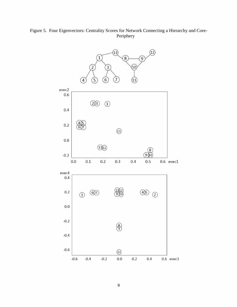
Figure 5 shows a network that contains two local substructures—a hierarchy and a core-periphery,

with one connection linking them. The eigenvalues are 2.47, 2.09, 1.41, 0.86, 0.62, 0, 0, 0, -0.64,

-1.41, -1.58, -1.62, -2.20, which suggest that three or possibly even four eigenvectors may be

useful. The magnitudes of these eigenvalues show less dramatic delineations between those that

are probably associated with substantial eigenvectors versus those that are associated with

eigenvectors that essentially convey noise. To proceed, the analysis might begin by examining the

four vectors, and if the fourth is meaningful, retain it, and if it does not seem to be interpretable or

helpful, retain only the first three. Thus, the information conveyed by the first four eigenvectors is

examined. (Recall the intention with this example is to demonstrate an example with more than

one or two eigenvectors.)

The first eigenvector in Figure 5 conveys volume information. Specifically, actors 8-10 have the

highest eigenvector centralities and three links each, which contrasts to actors 4-7 who have the

lowest eigenvector centralities and only one link each. The correlation with degree centralities,

9

Figure 5. Four Eigenvectors: Centrality Scores for Network Connecting a Hierarchy and Core-

Periphery

10

𝑟 = 0.678, is not perfect, given that actors 1-3 also have three links. However, their eigenvector

scores are a bit lower, but the design of an eigenvector was never intended to be wholly redundant

simply with degrees. (A first eigenvector is typically correlated with degree centrality, yet not

typically perfectly correlated, both findings are a result of the fact that the first eigenvector is

designed as an iteratively weighted function of actor degrees. Thus, it will be typically related to,

yet not completely redundant with, degree centralities.) The second eigenvector empirically

delineates other pattern information, such as portions of the hierarchy (i.e., actors 1-3 at the top of

the hierarchy versus those at the bottom, actors 4-7), the core (actors 8-10) versus the peripheral

(actors 11 and 12), and actor 13, the boundary spanner that links the sub-networks.

In the second plot in Figure 5, the third eigenvector further delineates the mapping of the left

portion of the hierarchy (actors 2, 4, 5) from the right (actors 3, 6, 7), with the core-peripheral

actors sitting at the center of this vector because they do not contribute to this distinction. The

fourth eigenvector contrasts actors 1, 8, and 13 (with negative indices) from the rest (whose indices

are positive), a difference that is interesting given that actors 1, 8, and 13 are precisely those that

play a substantial role in connecting the two local structures. Thus, a network analyst might wish

to include the fourth eigenvector as well.

Analogous to the investigation for the network in Figure 4, correlates were sought for the four

eigenvectors depicted for the network in Figure 5. The first eigenvector was correlated with degree

(r = 0.678), closeness (r = 0.447), and betweenness (r = 0.460). The second eigenvector was not

significantly correlated with any of these centrality scores (average r = 0.239). The third

eigenvector was not correlated with the traditional centrality scores (all r’s = 0.000). The fourth

eigenvector was not correlated with degree (𝑟 = −0.333), but it was significantly correlated with

closeness (𝑟 = −0.835 ) and betweenness (𝑟 = −0.824 ). Those latter two correlations were

sufficiently high as to give pause as to whether extracting four eigenvectors was overly much, as

the fourth eigenvector may be perhaps redundant with the first. However, the fourth eigenvector

was not entirely redundant with the first, as will be addressed and demonstrated shortly.

Next, dummy variables were created to capture other structural properties, specifically which

group an actor was in (group 1 was actors 1-7, group 2 was actors 8-13), whether an actor was a

spanner (yes for actors 1, 8, and 13), whether the actors existed in a clique (yes for actors 8, 9, 10),

whether actors had positions that were moderately between (yes for actors 1, 2, 3), and whether

actors were in a subgroup in the hierarchy to the left (subgroup one was actors 3, 6, 7; subgroup

two was actors 2, 4, 5). The findings follow:

The first eigenvector was significantly correlated with the group delineating whether they

were a part of the hierarchy or the core-periphery (r = 0.771), and the clique of actors 8-10

(r = 0.893).

The second eigenvector was correlated with these as well (group 𝑟 = −0.854, and clique

𝑟 = −0.711), and, in addition, reflected the actors who have moderate between positions

(actors 1, 2, 3, r = 0.745).

The third eigenvector reflected subgroup membership (r = 0.795 for the second group of

actors 2, 4, 5).

Regarding the issue of whether the fourth eigenvector was redundant with the first, it was

not, as it captured the roles of the spanners (actors 1, 8, 13), which is frequently an

important network diagnostic.

11

These investigations were intended as a reminder that multiple eigenvectors can provide greater

information than information contained in only a single eigenvector. Even these small networks

demonstrated that while occasionally a single eigenvector may be sufficient, in general, it may be

beneficial to extract multiple eigenvectors to enrich the profile of the actors’ positions within the

networks.

These examples have also been useful in illustrating the frequent observation that the first

eigenvector typically reflects volume as correlated with degree centrality. Second eigenvectors,

and those that follow, are designed mathematically to be orthogonal to, or uncorrelated with, the

first eigenvector, and, hence, are less likely to be correlated with standard network centrality

indices, such as degree. The information provided by the second eigenvector in Figure 4, and the

second, third, and fourth eigenvector in Figure 5 distinguished roles of actors in networks in a

manner more detailed than a reflection of volume, as important as volume is. In the section that

follows, it will be shown that in real (typically noisy) network data, a single eigenvector will seem

to be insufficient for fully capturing the information in the network.

Eigenvectors on a Real Social Network

In this section, the question is posed as to whether the multiple eigenvectors issue matters on a real

social network. The analysis examines the 32 actors in Freeman’s EIES (electronic information

exchange system) network (Freeman and Freeman, 1979, as measured at time 1), and it shall show

be shown that a single eigenvector would not provide a complete analysis of the patterns of the

social connections.

Freeman EIES Network

The 32×32 EIES network (Freeman and Freeman, 1979) was symmetrized by averaging the

sociomatrix values; 𝑿𝑠𝑦𝑚 =1

2(𝑿 + 𝑿′) . This matrix yielded ordered eigenvalues that begin:

46.89, 13.99, 8.54, 5.52, 3.93, 2.32, 1.87, 1.14, 0.27, 0.08, -0.16, and suggest that two eigenvectors

would be sufficient in capturing most of the network patterns. It may be the case that a network

scholar might believe that three (or more) eigenvectors would be necessary to capture the essence

of the patterns in the matrix. If there is uncertainty, the third vector can be examined to see if its

inclusion is necessary for the data description (or whether two eigenvectors may be sufficient),

considering the slight loss in parsimony if one were to proceed with three rather than two

eigenvectors. Each eigenvector could be correlated with any additional measures on the actors—

their positions or their attributes, to search for significant correlates and explanations of subsequent

vectors, which would strengthen the case for keeping them. Regardless, recall once again that the

main point is that in many applications, one vector might not be sufficient, so two or three, or

more, may be beneficial.

Figure 6 contains the plot of the 32 actors along the two eigenvectors. Without knowing any

content to describe the network, the fact that there is scatter in this plot indicates that there is more

12

Figure 6. Freeman Time 1, Two Eigenvectors

variability among these actors than was captured solely along the first eigenvector. The Freeman

EIES network is familiar to social network scholars, but its characterization by eigenvector

centrality has been insufficient. By definition, a second eigenvector brings new information to the

network analysis beyond the first.

Freeman’s EIES network was selected as an illustration in part because data on actor attributes are

available, and these might help interpret the eigenvector centralities. The actor attributes include a

researcher’s citation count and a dummy variable for the researcher’s discipline (sociology,

anthropology, statistics, or psychology). Thus the correlations among these eigenvectors, the actor

attributes, and the other traditional centralities of degree, closeness, and betweenness were

examined.

The correlations in Table 1 show the typical finding that the first eigenvector is rather highly

correlated with three standard measures of actor centrality: 𝑟 = 0.95 for degree, 𝑟 = −0.59 for

closeness, and 𝑟 = 0.62 for betweenness. (Also not unusual in real networks, these three indices

were somewhat correlated amongst themselves: 𝑟𝑑𝑒𝑔𝑟𝑒𝑒,𝑐𝑙𝑜𝑠𝑒 = −0.49, 𝑟𝑑𝑒𝑔𝑟𝑒𝑒,𝑏𝑒𝑡𝑤𝑒𝑒𝑛 = 0.69,

13

Table 1. Freeman Time 1 Network Correlates

Eigenvector Centralities

1 2

Degree 0.95*** .

Closeness -0.59* .

Betweenness 0.62*** .

Actor Attributes:

Citations . -0.48**

Sociology . -0.60*

Anthropology . 0.64***

Statistics . .

Psychology . .

*p<.01, ***p<.0001, “.” = n.s.

and 𝑟𝑐𝑙𝑜𝑠𝑒,𝑏𝑒𝑡𝑤𝑒𝑒𝑛 = −0.29.) In contrast, the second eigenvector was not at all redundant (not

significantly correlated) with the three other measures of actor centrality.

Next, note that the first eigenvector does not correlate with any of the actor attributes, nor did

degree centrality, closeness, or betweenness centrality correlate with the actor attributes. However,

the second eigenvector picks up an inverse relationship to citations and belonging to sociology,

and a positive association with anthropology.

Figure 7 depicts the relationship between the eigenvectors and the actor attributes. Using

regression to determine the location of the attributes (cf., Davidson 1983), the group of actors in

the “south” of the plot tend to be the sociologists, who are also more heavily cited, whereas the

anthropologists collect at the “north” of the plot. The correlations with the other disciplines,

statistics and psychology, were not significant. If they were to be represented, their locations would

be placed at the origin of the plot. Next, the “east” of the plot is marked by the degree and

betweenness centralities, consistent with their correlations with the first eigenvector (i.e., the east-

west axis). Closeness is also correlated with the first eigenvector, but the correlation is negative,

hence it is more towards the “west” of the plot.

Finally, as a check on the analyses, a singular value decomposition was also derived on the original

Freeman Time 1 network which was asymmetric; per 𝑿 = 𝑳𝑨𝑪, where 𝑳 contains the eigenvectors

of 𝑿𝑿′ , the matrix describing the similarities among the actors’ outgoing tendencies having

aggregated over their partner behaviors, 𝑪 contains the eigenvectors of 𝑿′𝑿, the matrix describing

the partners’ receiving tendencies, having aggregated over the actor initiatives, and 𝑨 contains the

singular values which are the square roots of the eigenvalues of the 𝑿𝑿′ and 𝑿′𝑿 matrices. The

first eigenvector of 𝑿𝑠𝑦𝑚 (plotted previously) was highly correlated with the first vector of 𝑿 in 𝑳,

𝑟 = 0.92, and the second eigenvector of 𝑿𝑠𝑦𝑚 was highly correlated with the second vector in 𝑳,

𝑟 = 0.97. Similarly, the first eigenvector of 𝑿𝑠𝑦𝑚 was highly correlated with the first vector in 𝑪,

𝑟 = 0.95, and the second eigenvector of 𝑿𝑠𝑦𝑚 was highly correlated with the second vector in 𝑪,

𝑟 = 0.97. Thus, little information seems to have been lost by treating the network as essentially

symmetric with mutual ties.

14

Figure 7. Freeman Time 1, Two Eigenvectors, with Actor Attributes

Discussion

When using eigenvector-based methods, such as principal components or factor analysis, social

and physical scientists often extract more than one vector or factor. To characterize one’s data

otherwise, is to leave much of it unexplained. In this paper, illustrations have been offered to help

support the recommendation that an extension beyond a single eigenvector should also apply to

the analysis of social networks.

In the social networks literature, the traditional emphasis is to focus on extracting a single

eigenvector to represent a centrality index. The current research considered whether the centrality

information derived from a first eigenvector is sufficient for capturing structure contained in social

networks. It was shown, in hypothetical and real data, that subsequent eigenvectors could provide

supplemental information.

15

When social scientists extract principal components or factors, no one would think to necessarily

limit themselves to a single factor (i.e., one is rarely sufficient). However, in typical application,

social networks scholars focus solely on the first eigenvector. It was shown that additional

eigenvectors may be informative in the world of social networks, and, therefore, they should also

be extracted and used for a richer understanding of the structure in the network. The first

eigenvector will typically be correlated with traditional measures of centrality, particularly degree.

Extracting a second, third, or more eigenvectors will necessitate further investigation as to the

nature of the structural patterns that the new eigenvectors reflect. Even in the simple networks

depicted in Figures 4 and 5, but also in the real EIES network depicted in Figures 6 and 7, several

classes of network structures and actor attributes were shown to have mapped onto the eigenvector

scores. This second step of analyses, used to help interpret the eigenvector scores, required

calculating correlation coefficients.

The first eigenvector, in any statistical application including the analysis of social ties, meets the

objective function of explaining the maximum amount of variance in the dataset. The second

eigenvector is derived to explain the maximum amount of remaining variance, subject to the

constraint that the resulting vector be orthogonal to, or uncorrelated with, the first eigenvector.

Thus, in social network analysis, while the first eigenvector centrality index is likely to be

correlated with the degree, closeness, and betweenness centralities, a multi-dimensional

eigenvector centrality, including the second eigenvector, and, if necessary, those that follow, will

be uncorrelated with the previous eigenvector(s) and therefore uncorrelated with the traditional

degree, closeness, and betweennness centralities as well. This lack of redundancy indicates the

supplemental information that the second and subsequent eigenvectors will bring to the network

modeler.

As when scholars use eigenvalues and eigenvectors in other arenas (e.g., principal components or

factor analysis), network scholars will have to balance the tradeoff of a more thorough

understanding of the data (in extracting more eigenvectors) and parsimony (in extracting fewer).

In some datasets, it may be the case that only a single eigenvector would be necessary to capture

the essence of the network (i.e., if the size of the first eigenvalue greatly dominates the others).

However, if two or more eigenvalues are large, relative to the others, it may prove beneficial to

examine whether the additional eigenvectors provide enlightening complementary information. If

the eigenvalues are only subtly different, it may be that the network scholar concludes that

extracting an additional eigenvector is not “worth it” considering the trade-off between the

additional value of more information explained versus the added complexity and reduced

parsimony.

Note that this research would also have implications for other centrality indices that are based on

eigenvectors, such as Bonacich’s power index (1987; 2007; Bonacich and Lloyd, 2001), and

Google’s Page Rank index (Brin and Page, 1998; Friedkin and Johnsen, 1990; Friedkin and

Johnsen, 2014). The eigenvector-based models have been expanded (e.g., for asymmetries,

Bonacich and Lloyd, 2001; and for non-binary and negative values, Bonacich, 2007), and further

developed, finessing parameters of the eigenvector values to weight indirect ties to a greater or

lesser extent (Bonacich, 1987), and each of these could be generalized as well.

16

As a practical matter, given the focus of social network analysis on solely the first eigenvector,

network scholars seeking to examine second, third, and subsequent eigenvectors will have to

circumvent network analysis packages. Network scholars seeking to extract multiple eigenvectors

can use software coding such as that provided in Appendix B.

This research described and illustrated the usefulness of a second, third, and possibly additional

eigenvectors, beyond the typical extraction and use of only the first eigenvector to capture

centrality and social network structural properties. If more than one eigenvalue is relatively large,

then the set of multiple eigenvectors contain more information than just the first, which tends to

reflect overall volume like degree centralities. In such cases, if the additional eigenvectors are not

used, information would be lost in the representation and understanding of the network patterns.

Social network data can be more challenging and effortful to gather than survey data which can

seem rather more straightforward. Accordingly, as much information should be extracted from the

network data as possible, and additional eigenvectors can enable this goal.

17

References

Bonacich, P. (1972), “Factoring and Weighting Approaches to Status Scores and Clique

Identification,” Journal of Mathematical Sociology, 2, 113-120.

Bonacich, P. (1987), “Power and Centrality: A Family of Measures,” American Journal of

Sociology, 92 (5), 1170-1182.

Bonacich, P. (2007), “Some Unique Properties of Eigenvector Centrality,” Social Networks, 29,

555-564.

Bonacich, P. and Lloyd, P. (2001), “Eigenvector-like Measures of Centrality for Asymmetric

Relations,” Social Networks, 23, 191-201.

Borgatti, S. (2005), “Centrality and Network Flow,” Social Networks, 27, 55-71.

Borgatti, S., Carley, K. M. and Krackhardt, D. (2006), “On the Robustness of Centrality Measures

under Conditions of Imperfect Data,” Social Networks, 28, 124-136.

Borgatti, S. and Everett, M. (1999), “Models of Core/Periphery Structures,” Social Networks, 21,

375-395.

Borgatti, S. and Everett, M. (2005), “A Graph-Theoretic Perspective on Centrality,” Social

Networks, 28 (4), 466-484.

Brin, S. and Page, L. (1998), “The Anatomy of a Large-Scale Hypertextual Web Search Engine,”

Computer Networks and ISDN Systems, 30, 107-117.

Comrey, A. L. (1962), “The Minimum Residual Method of Factor Analysis,” Psychological

Reports, 11, 15–18.

Costenbader, E. and Valente, T. W. (2003), “The Stability of Centrality Measures When Networks

are Sampled,” Social Networks, 25, 283-307.

Davidson, M. L. (1983), Multidimensional Scaling, New York: Wiley.

Freeman, L. (1978/1979), “Centrality in Networks: Conceptual Clarification,” Social Networks, 1,

215-239.

Freeman, S. C., and Freeman, L. C. (1979), “The Networkers Network: A Study of the Impact of

a New Communication Medium on Sociometric Structure,” Social Science Research

Reports No. 46, Irvine, CA, University of California.

Friedkin, N. E. (1991), “Theoretical Foundations for Centrality Measures,” American Journal of

Sociology, 96, 1478-1504.

Friedkin, N. E. and Johnsen, E. C. (2014), “Two Steps to Obfuscation,” Social Networks, 39, 12-

13.

Friedkin, N. E. and Johnsen, E. C. (1990), “Social Influence and Opinions,” Journal of

Mathematical Sociology, 15, 193-206.

Hoff, P. D., Raftery, A. E., and Handcock. M. S. (2002), “Latent Space Approaches to Social

Network Analysis,” Journal of the American Statistical Association, 97, 1090–1098.

Hoff, P. D., Ward, M. D. (2004), “Modeling Dependencies in International Relations Networks,”

Political Analysis, 12, 160-175.

Katz, L. (1953), “A New Status Index Derived from Sociometric Analysis,” Psychometrika, 18,

39–43.

Kim, J. and Mueller, C. W. (1978), Factor Analysis: Statistical Methods and Practical Issues,

Beverly Hills, CA: Sage.

Knoke, D. and Yang, S. (2007), Social Network Analysis, 2nd ed., Los Angeles, CA: Sage.

Kumbasar, E. (1996), “Methods for Analyzing Three-Way Cognitive Network Data,” Journal of

Quantitative Anthropology, 6, 15–34.

18

Manly, B. F. J. (1986), Multivariate Statistical Methods: A Primer, London: Chapman and Hall.

Namboodiri, K. (1984), Matrix Algebra, Los Angeles, CA: Sage.

Romney, A. K., Weller, S. C., and Batchelder, W. H. (1986), “Culture as Consensus: A Theory of

Culture and Informant Accuracy,” American Anthropologist, 88 (2), 313-338.

Rothenberg, R. B., Potterat, J. J., Woodhouse, D. E., Darrow, W. W., Muth, S. Q., and Klovdahl,

A. S. (1995), “Choosing a Centrality Measure: Epidemiologic Correlates in the Colorado

Springs Study of Social Networks,” Social Networks, 17, 273-297.

Scott, J. (2012), Social Network Analysis, 3rd ed., Los Angeles: Sage.

Seber, G. A. F. (1984), Multivariate Observations, New York: Wiley.

Smith, J. A. and Moody, J. (2013), “Structural Effects of Network Sampling Coverage I: Nodes

Missing at Random,” Social Networks, 35, 652-668.

Stephenson, K. and Zelen, M. (1989), “Rethinking Centrality: Methods and Examples,” Social

Networks, 11 (1), 1-37.

Tabachnick, B. G. and Fidell, L. S. (2006), Using Multivariate Statistics, 5th ed., Boston: Allyn &

Bacon.

Wang, X. and Sukthankar, G. (2015), “Link Prediction in Heterogeneous Collaboration

Networks,” in Missaoui, R. and Sarr, I. (eds.), Social Network Analysis—Community

Detection and Evolution, New York: Springer, 165-192.

Wasserman, S., and Faust, K. (1994), Social Network Analysis: Methods and Applications, New

York: Cambridge University Press.

Watts, D. J. and Strogatz, S. H. (1998), “Collective Dynamics of ‘Small-World’ Networks,”

Letters to Nature, 393 (4), 440-442.

Wright, B. and Evitts, M. S. (1961), “Direct Factor Analysis in Sociometry,” Sociometry, 24 (1),

82-98.

19

Appendix A

This appendix provides a refresher that demonstrates the traditional use of eigenvectors on

correlation matrices. Contrast two examples. First, Figure A1 presents a correlation matrix of six

variables that are all somewhat correlated. This pattern is not unusual when the variables all

represent slightly different wordings of a single, underlying concept being measured on a survey.

For example, say x1 is a survey item that asks, “How satisfied are you with today’s flight?” and

x2 asks, “How likely is it you would recommend our airline to your friends?” through to x6 which

asks, “How likely is it you will return to our airline the next time you need to fly?” These six

questions have much in common and are likely correlated; as one element of customer satisfaction

rises, others will likely follow suit. The eigenvalues of the matrix in Figure A1 (3.675, 0.578,

0.500, 0.500, 0.500, 0.247) show a sharp decline in magnitude after the first, suggesting that a

single eigenvector will capture the majority of the variance in the data. The entries in the

eigenvector indicate that the optimal means of combining these variables is essentially an average

(i.e., weighting x1 by 0.449 through x6 by 0.385).

By comparison, Figure A2 shows a correlation matrix among six variables in which two latent

concepts seem to have given rise to the data, one concept driving x1x3, another for x4x6.

For example, perhaps x1x3 are “satisfaction” questions as suggested previously, whereas in this

survey, perhaps the question x4 asks, “Do you believe the cost of your air travel was fair?” through

to x6 that might ask, “Do you think the price of your airline ticket was good value?” For these new

six questions, x1x3 will be highly correlated, each tapping the construct of satisfaction, and

x4x6 will be highly correlated, each reflecting a price assessment. Naturally, the two sets are

modestly correlated. The eigenvalues for this correlation matrix (3.052, 1.562, 0.408, 0.401, 0.292,

0.286) show a dramatic decline after the second, indicating the extraction of two eigenvectors

would be more fruitful than that of a single vector. The first eigenvector again suggests that much

of the structure of the matrix would be captured simply by an average of the six variables. The

second eigenvector delineates the two groups, with variables x1x3 having negative coefficients,

and x4x6, positive. (In principal components and factor analyses, of course, these initial

matrices are usually rotated to further clarify the structures, however the goal of simple structure,

objectively maximized by a a preponderance of zeros in the rotate matrix to represent constructs,

usually of variables, here of actors, seems less applicable, but certainly, in some uses, social

networks scholars may find a reason to do so; Kim and Mueller, 1978). If this analysis had

proceeded with only the first eigenvector, obviously the information contained in the second vector

would have been lost.

Table A1: Correlation Matrix with One Underlying Construct

x1 x2 x3 x4 x5 x6 eigenvector

x1 1.00 0.449

x2 0.70 1.00 0.414

x3 0.65 0.50 1.00 0.406

x4 0.60 0.50 0.50 1.00 0.399

x5 0.55 0.50 0.50 0.50 1.00 0.392

x6 0.50 0.50 0.50 0.50 0.50 1.00 0.385

20

Table A2: Correlation Matrix with Two Underlying Constructs

x1 x2 x3 x4 x5 x6 vector 1 vector 2

x1 1.00 0.416 -0.421

x2 0.70 1.00 0.409 -0.406

x3 0.65 0.60 1.00 0.401 -0.387

x4 0.20 0.20 0.20 1.00 0.392 0.473

x5 0.25 0.25 0.25 0.70 1.00 0.407 0.412

x6 0.30 0.30 0.30 0.65 0.60 1.00 0.423 0.339

In this paper, it was argued that this issue exists in analogous form for eigenvector centralities of

social network data. That is, sometimes one eigenvector can be sufficient, but often, additional

eigenvectors can provide useful complementary information.

21

Appendix B: SAS Code to Obtain Multiple Eigenvectors

proc iml;

x={ 0 1 0 0 0,

1 0 1 1 1,

0 1 0 0 0,

0 1 0 0 0,

0 1 0 0 0 }; *This matrix is the first in Figure 2.;

val=eigval(x); vect=eigvect(x); print val vect;

quit; run;

This code will derive the eigenvectors of the sociomatrix X. Alternatively, symmetric

sociomatrices could be submitted to principal components analyses in packages such as SPSS or

SAS. A principal component is merely an eigenvector with each element multiplied by the square

root of its eigenvalue. That is, a first component begins with the first eigenvector and multiplies

each element by the square root of the first eigenvalue (and a second component is the second

eigenvector multiplied by the square root of the second eigenvalue, etc.). This multiplication

essentially stretches the results to resemble ovals, with greater variance on the first axis than on

the second (to reflect that 𝜆1 > 𝜆2). Strictly speaking, the resulting components from SPSS or SAS

should be scaled back to return to their original eigenvectors. To obtain the original eigenvectors,

the elements in the components loadings matrix would be divided by the square roots of their

respective eigenvalues. However, given that one is a function of the other, they are perfectly

correlated, so reporting two or three components rather than two or three eigenvectors would not

be misleading, because the ordering of the actors along either the vector or the component would

be the same.