eindhoven university of technology master sensor … · eindhoven university of technology ... the...

Eindhoven University of Technology

MASTER

Sensor fusion

Wittrock, E.P.

Award date:1996

DisclaimerThis document contains a student thesis (bachelor's or master's), as authored by a student at Eindhoven University of Technology. Studenttheses are made available in the TU/e repository upon obtaining the required degree. The grade received is not published on the documentas presented in the repository. The required complexity or quality of research of student theses may vary by program, and the requiredminimum study period may vary in duration.

General rightsCopyright and moral rights for the publications made accessible in the public portal are retained by the authors and/or other copyright ownersand it is a condition of accessing publications that users recognise and abide by the legal requirements associated with these rights.

• Users may download and print one copy of any publication from the public portal for the purpose of private study or research. • You may not further distribute the material or use it for any profit-making activity or commercial gain

Take down policyIf you believe that this document breaches copyright please contact us providing details, and we will remove access to the work immediatelyand investigate your claim.

Download date: 14. Jul. 2018

Eindhoven University of TechnologyDepartment of Electrical EngineeringMeasurement and Control Group

SENSOR FUSION

E.P. Wittrock

M.Sc.ThesisCarried out from February 1996 to October 1996Commissioned by Prof. dr. ir. P.P.I. van den BoschUnder supervision of Dr. S. Weiland and ir. R. KunstEindhoven, 10 October 1996

The department of Electrical Engin~ering of the Eindhoven University of Technology accepts no responsibility forthe contents of M.Sc. Theses or reports on practical training periods.

Summary

Wittrock, E.P.;Sensor FusionM.Sc. Thesis, Measurement and Control Group MBS, section ER, Electrical Engineering,Eindhoven University of Technology, The Netherlands, Oct. 1996.

Sensor fusion is used to combine sensor measurements with different properties to form aresulting measurement that may not be possible from one single sensor alone. Objective ofthis report is to find methods, and compared them with each other, to fuse several sensorsignals. Applications in the section ER are in two projects. The first project needs to measurethe deck position of a schip and the second project needs to measure the position of a bus ona bus lane. This report describes discrete time Kalman filter based algorithms used for SensorFusion. Several approaches have been proposed and defined. The covariance based algorithmsare used to fuse two or more separate sensor measurements and merge them to one entity. Thevarious fusion algorithms are implemented in Matlab files and the performance of thealgorithms are evaluated through computer simulations with a one-dimensional dynamicmodel, with a assumed acceleration acting on the position and speed. It is shown that thedefined fusion algorithms give similar results under various sensor configurations and sensorvariances. Also investigated is the effect of bias on the various fusion algorithms. A proposalis done to solve the sensor fusion problem with a H", filter, to enable us to take into accountthe sensor properties with weighting functions in the frequency domain.

Samenvatting

Wittrock, E.P.;Sensor FusieAfstudeerverslag, vakgroep MBS, sectie ER, Faculteit Elektrotechniek, Technische UniversiteitEindhoven, Okt. 1996.

Sensor fusie word gebruikt om verscheidene sensor metingen met verschillende eigenschappente combineren tot een resultaat dat niet kan worden bereikt met een enkele sensor.Doelstelling van dit raport is methoden te vinden, en met elkaar te vergelijken, omverschillende sensor signalen the fuseren. Toepassingen voor deze vakgroep zijn er voor eentweetal projecten. Het eerste project is de bepaling van een dekstand van een schip en bij hettweede project is het van belang de positie van een bus op een busbaan zeer nauwkeurig tebepalen. Dit rapport beschrijft Kalman filter algoritmen, in de discrete tijd, gebruikt om desensor metingen te fuseren. Verscheidene methoden zijn voorgesteld en gedefinieerd. De opcovariantie gebaseerde algoritmen worden gebruikt om twee of meerdere verschillende sensormetingen te fuseren tot een gezamenljjk resultaat. De verscheidene fusie algoritmen zijngei"mplementeerd in Matlab files en de prestaties van de algoritmen zijn geevalueerd metbehulp van computer simulaties met een 1-dimensionaal dynamisch model, met eenversnelling die inwerkt op de snelheid en de positie. De simulaties laten zien dat dealgoritmen hetzelfde resultaat geven met verscheidene sensor configuraties en sensorvarianties. Ook is er gekeken naar het effect van bias op de verscheidene fusie algoritmen.Er wordt een voorstel gedaan om het sensor fusie probleem op. de lossen met een Hoo filter,op een equivalente manier als het Kalman filter, waardoor we de sensor eigenschappen in hetfrequentie bereik kunnen meenemen in de weegfuncties.

October 10, 1996 Sensor Fusion 3

TABLE OF CONTENTSList of abbreviations 5

Chapter 1. Introduction 7

Chapter 2. System model 9

Chapter 3. Central fusion 113.1. Selection calculation method 13

Chapter 4. Hierarchical fusion. . . . . . . . . . . . . . . . . . . . . . . . . . . . . . . . . . . . . . .. 154.1. Derivation of the hierarchical fusion algorithm 164.2. Comparing the hierarchical fusion with the central fusion 19

Chapter 5. Hierarchical fusion with feedback 215.1. Derivation of the hierarchical fusion with feedback algorithm 225.2. Comparing the hierarchical feedback fusion with the central fusion 235.3. Reduced communication requirements 24

Chapter 6. Distributed model architecture . . . . . . . . . . . . . . . . . . . . . . . . . . . . . . .. 276.1.Derivation of the distributed fusion algorithm 29

Chapter 7. Hoo filtering 31

Chapter 8. Simulations. . . . . . . . . . . . . . . . . . . . . . . . . . . . . . . . . . . . . . . . . . . .. 358.1. Simulation model 358.2. Two position sensors 378.3. One position sensor and one speed sensor 438.4. multiple position sensors and unknown input u 468.5. Detecting a fault sensor 53

Chapter 9. Conclusions. . . . . . . . . . . . . . . . . . . . . . . . . . . . . . . . . . . . . . . . . . . .. 55

References 57

Appendix A: kost.m 59

Appendix B: makedat.m . . . . . . . . . . . . . . . . . . . . . . . . . . . . . . . . . . . . . . . . . . .. 61

Appendix C: central.m and centr82.m 63

Appendix D: hier.m and hier82.m .. . . . . . . . . . . . . . . . . . . . . . . . . . . . . . . . . . .. 65

Appendix E: hierfeed.m and hierfe82.m . . . . . . . . . . . . . . . . . . . . . . . . . . . . . . . .. 67

Appendix F: hierred.m and hierre82.m . . . . . . . . . . . . . . . . . . . . . . . . . . . . . . . . .. 69

October 10, 1996

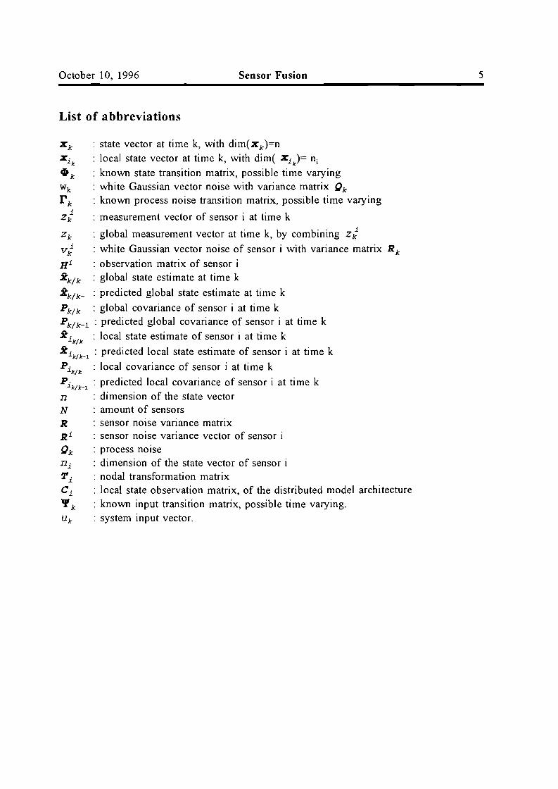
List of abbreviations

Sensor Fusion 5

JCk : state vector at time k, with dim(JCk)=nJCik : local state vector at time k, with dim( JCi )= n j

• k : known state transition matrix, possible time varyingwk : white Gaussian vector noise with variance matrix 'hr k : known process noise transition matrix, possible time varying

z1 : measurement vector of sensor i at time k

Zk : global measurement vector at time k, by combining z1v1 : white Gaussian vector noise of sensor i with variance matrix R k

Hi : observation matrix of sensor iXk / k : global state estimate at time k

Xk / k - : predicted global state estimate at time k

Pk / k : global covariance of sensor i at time kPk / k-l : predicted global covariance of sensor i at time k

Xik/k

: local state estimate of sensor i at time k

Xik/k

_1

: predicted local state estimate of sensor i at time k

Pik/k

: local covariance of sensor i at time k

Pi / : predicted local covariance of sensor i at time kk k-l

n : dimension of the state vectorN : amount of sensorsR : sensor noise variance matrixR i : sensor noise variance vector of sensor iOk : process nOisen i : dimension of the state vector of sensor i'I'i : nodal transformation matrixCi : local state observation matrix, of the distributed model architecture1pk : known input transition matrix, possible time varying.Uk : system input vector.

October 10, 1996

Chapter 1. Introduction

Sensor Fusion 7

Using different types of sensors to obtain information allows the advantages of one sensortype to compensate for the disadvantages of another and further provides redundancy,increasing system robustness.In this report different kinds of architectures for multi-sensor data fusion will be discussed:• In the centralized fusion architecture [chapter 3] all the raw sensor data is transmitted tothe fusion agent. The main advantage is that the algorithm is simple and is conceptuallysimilar to single sensor algorithm. A disadvantage of this approach may be the highcomputational load of the central processor.

Figure 1, centralizedfusion

• The hierarchical architecture [chapter 4], frequently referred to as the sensor level trackingin which each sensor maintains its own track full based on its own data.

FigUl'e 2, hierarchicalfusion

The tracks from the various sensors are transmitted to a single central processor which isresponsible for fusing the tracks to form a global estimate. An advantage is that it is easier

8 Sensor Fusion 10 October 1996

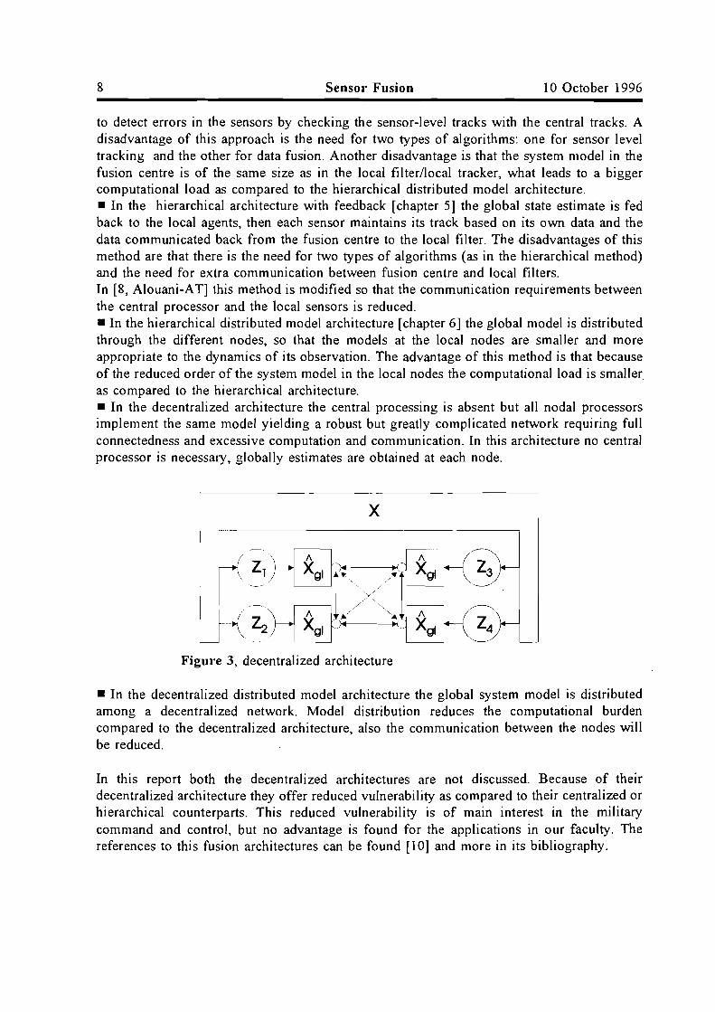
to detect errors in the sensors by checking the sensor-level tracks with the central tracks. Adisadvantage of this approach is the need for two types of algorithms: one for sensor leveltracking and the other for data fusion. Another disadvantage is that the system model in thefusion centre is of the same size as in the local filter/local tracker, what leads to a biggercomputational load as compared to the hierarchical distributed model architecture.• In the hierarchical architecture with feedback [chapter 5] the global state estimate is fedback to the local agents, then each sensor maintains its track based on its own data and thedata communicated back from the fusion centre to the local filter. The disadvantages of thismethod are that there is the need for two types of algorithms (as in the hierarchical method)and the need for extra communication between fusion centre and local filters.In [8, Alouani-AT] this method is modified so that the communication requirements betweenthe central processor and the local sensors is reduced.• In the hierarchical distributed model architecture [chapter 6] the global model is distributedthrough the different nodes, so that the models at the local nodes are smaller and moreappropriate to the dynamics of its observation. The advantage of this method is that becauseof the reduced order of the system model in the local nodes the computational load is smalleras compared to the hierarchical architecture.• In the decentralized architecture the central processing is absent but all nodal processorsimplement the same model yielding a robust but greatly complicated network requiring fullconnectedness and excessive computation and communication. In this architecture no centralprocessor is necessary, globally estimates are obtained at each node.

x

Figure 3, decentralized architecture

• In the decentralized distributed model architecture the global system model is distributedamong a decentralized network. Model distribution reduces the computational burdencompared to the decentralized architecture, also the communication between the nodes willbe reduced.

In this report both the decentralized architectures are not discussed. Because of theirdecentralized architecture they offer reduc.ed vulnerability as compared to their centralized orhierarchical counterparts. This reduced vulnerability is of main interest in the militarycommand and control, but no advantage is found for the applications in our faculty. Thereferences to this fusion architectures can be found [10] and more in its bibliography.


Chapter 2. System model

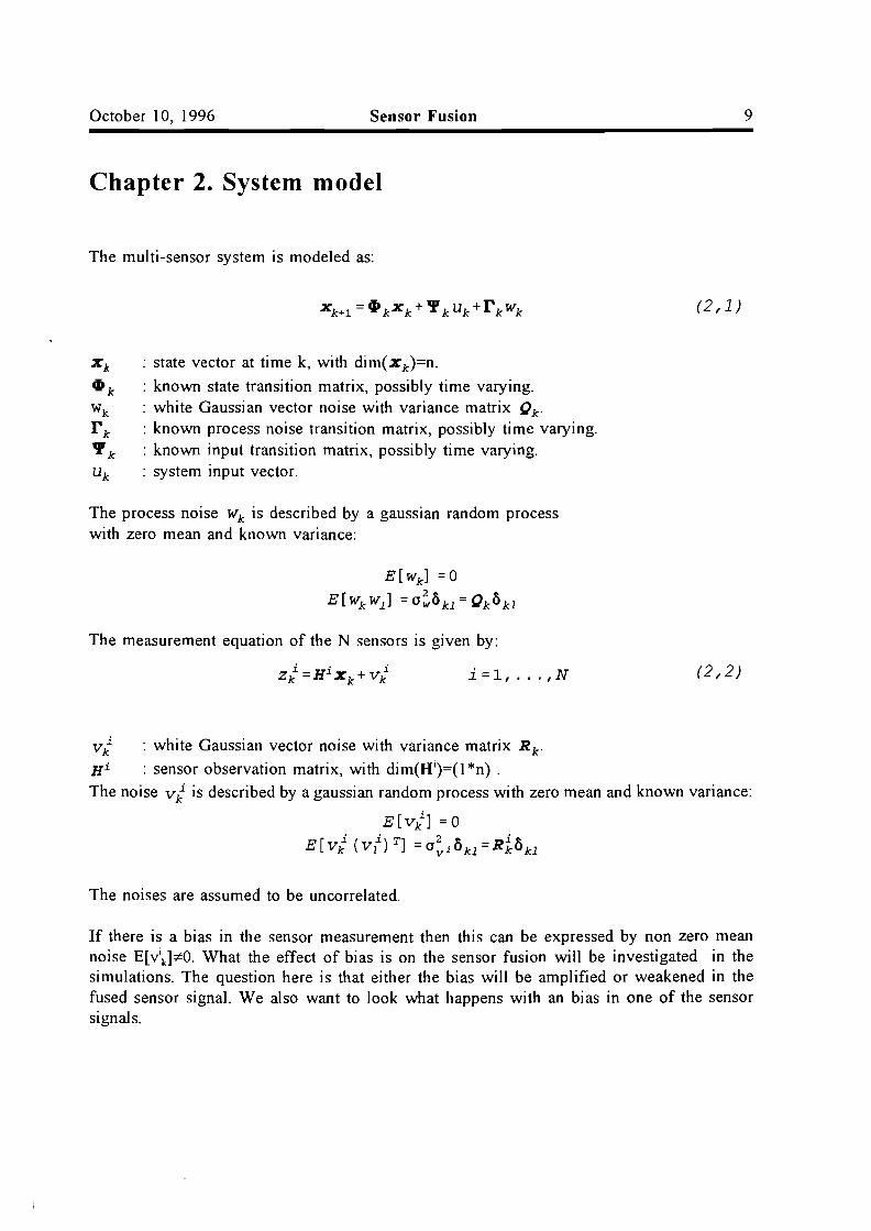
The multi-sensor system is modeled as:

Xl< : state vector at time k, with dim(xk)=n.

• k : known state transition matrix, possibly time varying.wk : white Gaussian vector noise with variance matrix 'h.r k : known process noise transition matrix, possibly time varying.'1' k : known input transition matrix, possibly time varying.Uk : system input vector.

The process noise wk is described by a gaussian random processwith zero mean and known variance:

E[wk ] =0

E[WkW1 ] =(J~Okl=QkOkl

The measurement equation of the N sensors is given by:

(2,1)

j=l,,,.,N (2,2)

vj : white Gaussian vector noise with variance matrix R k .

Hi : sensor observation matrix, with dim(H i)=(1 *n) .

The noise vj is described by a gaussian random process with zero mean and known variance:

E[vj] = 0

E[vj (v/) T] =(J~iOkl=R~Okl

The noises are assumed to be uncorrelated.

If there is a bias in the sensor measurement then this can be expressed by non zero meannoise E[Vik];t:O. What the effect of bias is on the sensor fusion will be investigated in thesimulations. The question here is that either the bias will be amplified or weakened in thefused sensor signal. We also want to look what happens with an bias in one of the sensorsignals.


Chapter 3. Central fusion

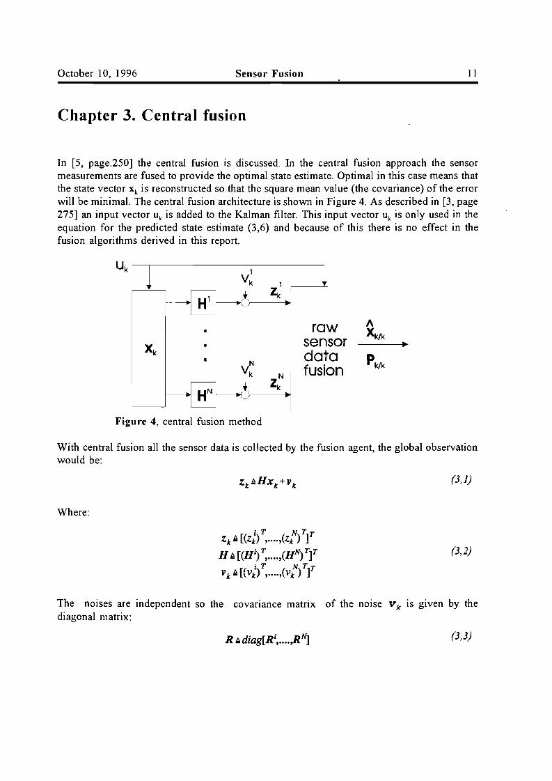
In [5, page.250] the central fusion is discussed. In the central fusion approach the sensormeasurements are fused to provide the optimal state estimate. Optimal in this case means thatthe state vector X k is reconstructed so that the square mean value (the covariance) of the errorwill be minimal. The central fusion architecture is shown in Figure 4. As described in [3, page275] an input vector Uk is added to the Kalman filter. This input vector Uk is only used in theequation for the predicted state estimate (3,6) and because of this there is no effect in thefusion algorithms derived in this report.

Uk-l 1 1Vk 1

Zkc*

raw A~/ksensor ...

Ndata Pk/kVk N fusion

y Zk

Figure 4, central fusion method

With central fusion all the sensor data is collected by the fusion agent, the global observationwould be:

(3,1)

Where:

(3,2)

The noises are independent so the covariance matrix of the noise v k is given by thediagonal matrix:

(3,3)


The global estimate and covariance with all the sensor data is given by:

Xk/k=Xkjk-l +Kk(Zk-HXk/k-l)

with Kk=Pk/kHTR-1

and:

(3,4)

(3,5)

The predicted estimate and the predicted covariance can be computed from the extrapolationequations:

and:

X =() x +. Uk/k-l k-l k-l/k-l k-l k-l(3,6)

(3,7)

The Kalman gain K k and the covariance matrix Pk / k can be written in two ways. In the way

used above the Kalman gain K k = Pk / kHT R-1 is calculated with the covariance matrix. So the

covariance matrix is calculated first. These equations are derived from the equations below,where the Kalman gain has to be calculated first with the predicted covariance matrix.Subsequently the covariance matrix can be calculated with the calculated Kalman gain.

(3,8)

(3,9)

With the equations above the result are two slightly different recursive loops for calculatingthe global estimate and the global covariance. With simple substitutions it can be seen thatthe result is the same. The equations for the two slightly different recursive loops are givenin this report because in the literature they are both used in the referred literature. The orderof calculating is shown in Table I.


Table I,Difference between recursive calculations

method 1 equations 1 method 2 equations 2

~k/k-l (3, 6) ~k/k-l (3, 6)

P k/k - 1 (3, 7) P k/k - 1 (3, 7)

Pk / k (3, 5) Kk (3, 8 )

Kk (3, 4 ) Pk / k (3, 9)

~k/k (3, 4 ) ~k/k (3, 4 )

3.1. Selection calculation method

Selecting one of the two recursive calculation, method 1 and method 2 can be based on twocriterion namely the numerical stability of the equations and the difference in calculation timenecessary for one calculation loop.

A disadvantage of method 1 can be the extra inverse of Pk/k-t introduced in equation (3,5).If Pk/k-, becomes very small this inverse can lead to numerical instabilities, and method 2 willhave the preference. A reason to choose for method 1 can be a smaller calculation timecompared to method 2.

To calculate the difference in calculation time we want to look at the proportion (V) betweenone calculation loop of method 1 and one calculation loop of method 2. The calculation timeexist of a collective part (A) that exists of the calculation made by equations (3,4), (3,6) and(3,7). The additional calculations (B) for method 1 that are given by K k in equation (3,4), andequation (3,5) and the additional calculations (C) for method 2 are given by the equations(3,8) and (3,9). A multiplication of (m*n) matrix with a (n*p) matrix is of the order O(m*n*p)and the inverse of a (n*n) matrix is of order 0(0.7*n3

). The value 0.7 is estimated with helpof Matlab. Addition of matrixes are not taken in account because they are of lower order andfaster than multiplications.

A=2n 3 +2n 2 +n+2NnB=2N2n+2Nn 2+1.4n 3

C=3Nn 2 +2N2n+0.7N 3 +n 3

V Gl Tmethod2 =A +CT method 1 A + B

(3,10)

The proportion V is defined by the time necessary for method 2 divided by the time necessaryfor method 1. With the proportion V we can easily conclude whether method 1 or method 2


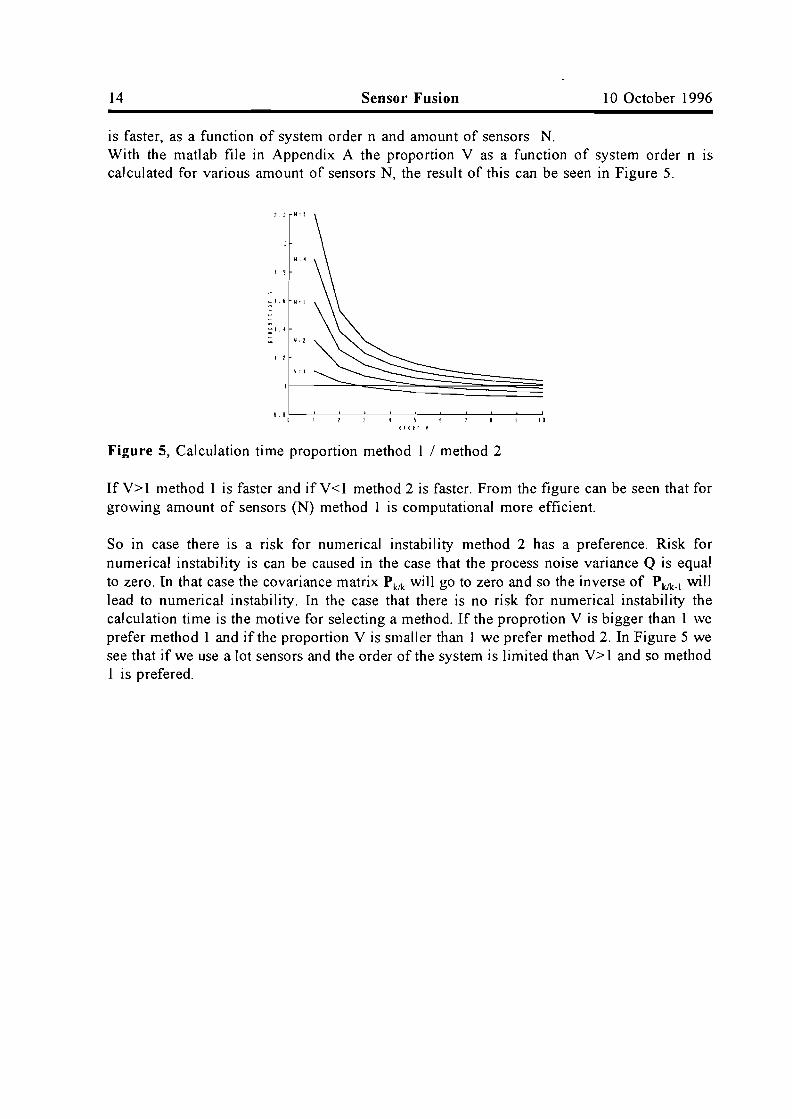
is faster, as a function of system order n and amount of sensors N.With the matlab file in Appendix A the proportion V as a function of system order n IS

calculated for various amount of sensors N, the result of this can be seen in Figure 5.

2.2 loId

10\order n

lr4 ~ 1

, ,

<, .6 IoI:J

--c.

:1 1

- N: 2-I 1

N: 1

O. ,0

Figure 5, Calculation time proportion method I / method 2

If V> 1 method 1 is faster and if V<1 method 2 is faster. From the figure can be seen that forgrowing amount of sensors (N) method I is computational more efficient.

So in case there is a risk for numerical instability method 2 has a preference. Risk fornumerical instability is can be caused in the case that the process noise variance Q is equalto zero. In that case the covariance matrix P klk will go to zero and so the inverse of Pkik-1 willlead to numerical instability. In the case that there is no risk for numerical instability thecalculation time is the motive for selecting a method. If the proprotion V is bigger than 1 weprefer method 1 and if the proportion V is smaller than I we prefer method 2. In Figure 5 wesee that if we use a lot sensors and the order of the system is limited than V> 1 and so method1 is prefered.


Chapter 4. Hierarchical fusion

In [9, Sun-H] an algorithm for the hierarchical fusion is proposed. The new fusion algorithmis obtained by further derivation of the centralized fusion algorithm. First the algorithm willbe presented and discussed, subsequently the algorithm will be derived and also comparedwith the central fusion algorithm.

Vk

1

All

'~ ~*\}----j-I-=-Z-=kl:~'-:Io::c~a-I~~Xk/k Pk/kI ~J 'filter 1 All

Xk/k-1 Pk{k-l

Figure 6, hierarchical fusion method

1

fusioncenter

Ax.vk

The hierarchical fusion method needs two types of processing nodes:• Local tracking node. The purpose of the local tracking node is to obtain a local stateestimate and a local covariance. The local state estimates are all of the same order as theglobal state estimate, namely order n. A way of reducing this order is discussed in chapter 6.• Data fusion centre. This centre fuses the local estimates to a global estimate, with help ofthe local covariances.

In the local node the filter processes data from a local sensor to generate a local state estimation. At each time k the local agents transmit the local state estimate and the predicted localstate estimate, as well as the corresponding covariances to the fusion agent. It is not necessaryto communicate the predicted local state estimate and predicted local covariance to the fusioncentre because they can also be calculated in the fusion centre with the local state estimateand the local covariance. If the predicted local state estimate and the predicted localcovariance are calculated in the fusion center you make a trade between extra calculation atthe fusion center and less communication between local filter and the fusion center.In the fusion centre, the local state estimates are fused with the predicted global state estimateto produce a global state estimate. This fusion is weighted with the local covariances and theglobal covariance. The predicted global state estimate and the predicted global covariance areobtained with the extrapolation equations (3,6) and (3,7). To calculate the predicted globalstate estimate you need to connect the input Uk to the fusion center, this is caused by the needfor Uk in equation (3,6)..


According to [5, page 255] the data fusion equations in the data fusion centre can be writtenas:

N

P;~Xklk=P;~-l Xk/k-l +L (P~J-l X~k - (p~k_lrl X~k-l)j;l

N

P;~ =P;~-l +L (P~J-l -(P~k_l)-l)j;l

(4,1)

(4,2)

Further derivation [9, Sun-H] the data fusion equations will give the following equations forthe global state estimate:

This equation expresses that the global state estimate equals the sum of the global stateprediction and an update. This update involves two terms. One is the sum of the differencesbetween each local state estimate and fusion prediction, weighted by the inverse of thecorresponding local sensor covariance. The other one is the sum of the differences betweenthe fusion prediction and each local sensor prediction, weighted by the inverse of thecorresponding local sensor prediction covariance. The sum of the two terms is weighted byfusion state covariance. '

The global covariance is calculated according to equation (4,2) , and the predicted globalestimate and the predicted global covariance are calculated with the extrapolation equations(3,6) and (3,7).

4.1. Derivation of the hierarchical fusion algorithm

The purpose of the fusion centre is to calculate the global estimate and the global covariancewith help of the local estimates, local covariances, predicted global estimate and predictedglobal covariance. The hierarchical fusion algorithm can be derived by substitutions of thelocal estimator equations in the central fusion equations.

The local estimate and covariance are calculated with:

(4,4)

(4,5)

The global estimate is calculated with equation (3,4) and the global covariance is calculated

October 10, 1996

with equation (3,5).

Sensor Fusion 17

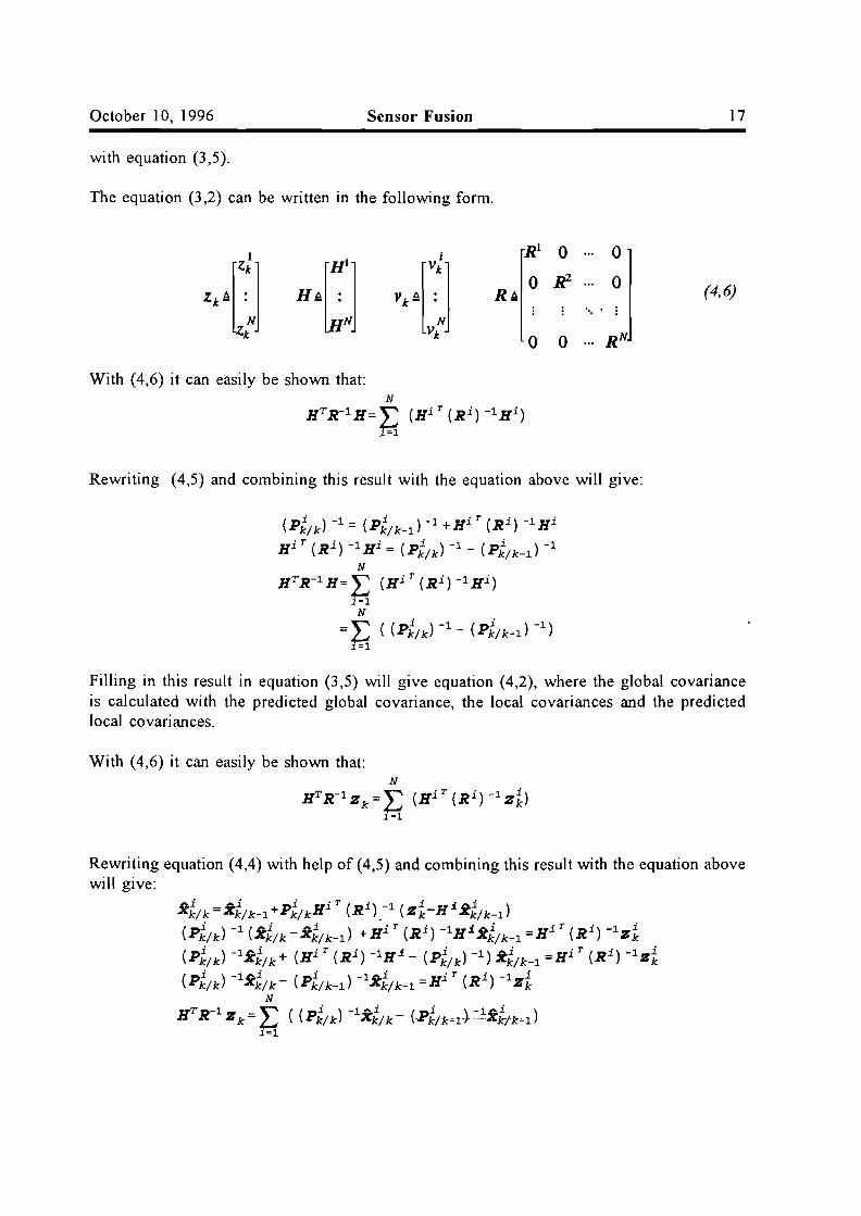
The equation (3,2) can be written in the following form.

1

~~]R1 0 ... 0

[' [1 0 If- ... 0

Z.' :N HA :N VtA RA~.. -

"t 0 0 ... RN.

With (4,6) it can easily be shown that:N

H T R-1 H=}::; (Hi T (R i ) -1 Hi)~=1

Rewriting (4,5) and combining this result with the equation above will give:

(P;/k) -1 = (P;/k-1) -1 +Hi T (R i ) -lHi

Hi T (R i ) -1 Hi = (P;/k) -1 - (P;/k-1) -1N

H T R-1 H= L (Hi T (Ri ) -lHi )i=l

N

=}::; ((P;/k) -1 - (P;/k-1) -1)~=1

(4,6)

Filling in this result in equation (3,5) will give equation (4,2), where the global covarianceis calculated with the predicted global covariance, the local covariances and the predictedlocal covariances.

With (4,6) it can easily be shown that:N

H T R- 1 Zk

=}::; (HiT(Ri)-lZ~)~=1

Rewriting equation (4,4) with help of (4,5) and combining this result with the equation abovewill give:


Now we will rewrite equation (3,4) so that we can fill in the equation above. The result isequation (4,1).

With help of equations (4,1) and (4,2) and a more convenient equation for the global stateestimate is derived:

N-1 -1 ~ (( i ) -1 (i ) -1)Pk/k =Pk/ k -1 +~ Pk/ k - Pk/ k -1

~=1

N-1 A _ -1 A ~ (( i ) -1 (i ) -1) A

Pk / k A.k/k-1 -Pk/k-1Xk/k-1 +.(..J Pk/ k - Pk/ k - 1 A.k/k -1~=1

N

P -1 A _ p-1 A ~ ( (pi ) -1 Ai (pi ) -1 Ai )k/k-1 A.k/k-1 - k/kA.k/k - .(..J k/k A.k/k - k/k-1 A.k/k-1

~=1

N

P -1 A -1 A ~((pi )-lAi (i )-l A i )k/kXk/k =Pk / kXk/k-1 + .(..J k/k Xk/ k - Pk/ k-1 A.k/k-1 +

~=1

N

-l: ((Pt/k) -litk/ k _1 - (Pt/k-1) -litk/ k _1)~=1

N N

itk/k=Xk/k-1 +Pk/k~ ((Pt/k) -1 (Xt/k-Xk/k-J )+Pk/k~ ((Pt/k-1) -1 (itk/ k- 1 -itt/k-1))~=1 ~=1

The result of this derivation is equation (4,3), and so we showed how the fusion equations ofchapter 4 are derived.

October 10, 1996 Sensor Fusion

,

19

4.2. Comparing the hierarchical fusion with the central fusion

In this section the global state estimate and the global covariance of the central fusionalgorithm will be compared with the global state estimate and the global covariance of thehierarchical fusion algorithm in the two sensor case with equal observation matrixes and equalsensor noise variances. The assumptions done for comparing the central fusion with thehierarchical fusion are that we use two similar sensors, consequently: N=2, H]=H2 , R]=R2.

The comparison in this section is done for a very special case. If we compare other cases like,more than two sensors (n>2), different observation matrices Hi';t:Hj or different sensorvariances Rj:;t:Rj the equations would be to extensive to be compared as in this section. So theother cases are examened with simulations further on in this report.With the assumptions done we will show that the global state estimate of the central fusionalgorithm is equal to the global state estimate of the hierarchical fusion algorithm, as well thatthe global covariance of the central fusion algorithm is equal to the global covariance of thehierarchical fusion algorithm:

?~..central :..- L'-.hier.Kk/k -Xk/k

?,...central :..- ..hier.rk/k -.Yk/k

First we will calculate the global covariance with the central fusion equation (3,5).-1 -1 T -1

Pk / k =Pk/ k -1 +H R H

[R-1

0 ][H]-1 -1 T 1 1

Pk/k=Pk/k-1 +[H1 Hi) 0 R~l H2

-1 -1 T -1 T -1P k/ k =Pk/ k -1 +H1R 1 H1 +H2 R 2 H2

-1 -1 T -1Pk/ k = Pk/ k -1 + 2 H1R1 H1

Then the global covariance is calculated with the hierarchical fusion equation (4,2). Asexpected the result is the same as calculated before with the central fusion equation.

2

P"k7k=Pk:7k-1 +.r: ((Pt;k) -1_ (P~/k-1) -1)~=1

2

P"k7k=P"k7k-1 +~ (Hi T (R i ) -lHi )~=1

-1 -1 ..PI T ( 1) -1 ..PIPk/k=Pk/k-1 +2n- R n-

If the global state estimate is calculated with the central fusion equation (3,4) in the twosimilar sensor case the result will be as follows:

20

,

Sensor Fusion 10 October 1996

With equations (4,4) and (4,5) we obtain the following expressions which will be combinedwith the equation for the global state estimate of the hierarchical fusion algorithm.

(pi ) -lAi (pi ) -lAi Hi T (Ri) -1 ik/k A.k/k- k/k-1 A. k/k-1 = Zk(P1/k-1) -1 - (P1/k) -1 = -Hi T (Ri ) -lHi

Then the global state estimate is calculated with the hierarchical fusion equation (4,3)

itk/ k =itk/ k-> + Pk/k(t (pLk) -> (itt/k - itk/k-» +t, (Pt/H) -> (itk/k-> -itt/H) J2

Xk/ k ="k/k-1 + Pk/k.E (P1/k) -lx 1/k- (pLk-1) -1,,1/k_1 + ( (P1/k-1) -1_ (P1/k) -1) "k/k-1)~=1

2

Xk/ k ="k/k-1 +Pk/kL (HiT (Ri ) -l z t-HiT

(R i ) -lHixk/k_1)i=l

"k/k="k/k-1 +Pk/ k (JtlT (R1) -1 (zl+z~) -2H1T

(R1) -lJtl"k/k_1)

It can be seen that the result of the global state estimate with the central fusion algorithm iscorresponding with the result with the hierarchical fusion algorithm.


Chapter 5. Hierarchical fusion with feedback

In [5, page 252] the hierarchical fusion with feedback is presented. The local estimates arecommunicated to a central location where data fusion is performed, subsequently the fuseddata is communicated back to the local agents where it is used as priori statistics.

Uk1 All

Vk ~k Pk/klocal

filter 1A~k Pk/k

A

fusion xk/kcenter Pk/kN AN N

VkZN Xk/k Pk/k

localk

filter NAXk/k Pk/k

Figure 7, hierarchical fusion with full feedback

The local state estimate and local covariance are calculated in the local filters with the sameequations as used in the hierarchical fusion method, namely equation (4,4) and equation (4,5).The difference with the hierarchical fusion method is that in this case the local filters use theglobal state estimate of the fusion center to calculate the predicted local state estimate.

The fusion equations with feedback are:

N

P;~XtJk=L ((P~J-I X~J - (N-l)P;~_1 XtJk-1i=l

(5,1)

N

P;~= L ((P~J-I) -(N-l)P;~_1i"'l

(5,2)

A more convenient way of writing the equation for the global state estimate is given inequation (5,3).

N

XtJk =XtJk-1+PtJkL ((p~J-I(X~k-XtJk-I))i"'l

(5,3)

The predicted global estimate and the predicted global covariance can be computed from theextrapolation equations (3,6) and (3,7). Because of equations (3,6) the input Uk must beconnected to the fusion center.


5.1. Derivation of the hierarchical fusion with feedback algorithm

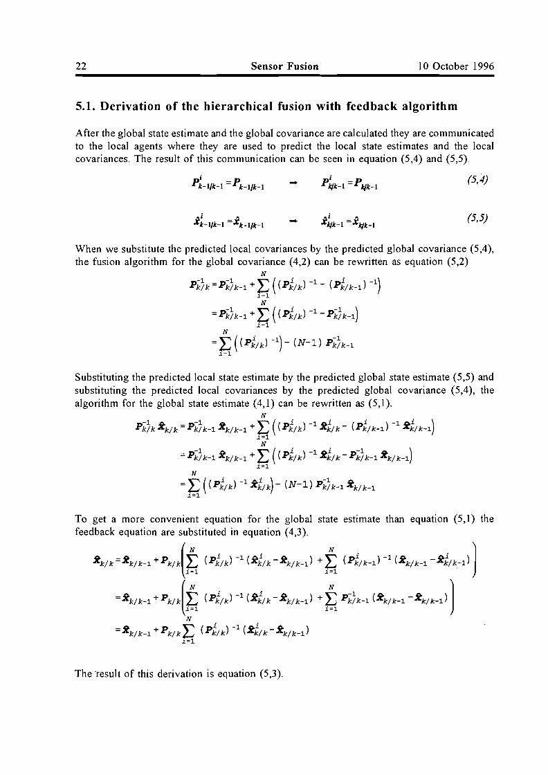
After the global state estimate and the global covariance are calculated they are communicatedto the local agents where they are used to predict the local state estimates and the localcovariances. The result of this communication can be seen in equation (5,4) and (5,5).

Ai AXk-l/k-l =Xk- 1/k- 1

--

(5,4)

(5,5)

When we substitute the predicted local covariances by the predicted global covariance (5,4),the fusion algorithm for the global covariance (4,2) can be rewritten as equation (5,2)

N

-1 -1 ~ (( i ) -1 (i ) -1)Pk/ k =Pk/ k-1 + 4.J Pk/ k - Pk/ k-1~-1

N-1 ~ (( i ) -1 -1 )=Pk/k-1 +.(....J Pk/k -Pk/ k-1

~-1

N

=I: ((Pt/k) -1)_ (N-l) Pic7k-1~-1

Substituting the predicted local state estimate by the predicted global state estimate (5,5) andsubstituting the predicted local covariances by the predicted global covariance (5,4), thealgorithm for the global state estimate (4,1) can be rewritten as (5,1).

N

pic7kXk/k=Pic7k-1 Xk/ k-1 +I: ((Pt/k) -1 Xt/k- (Pt/k-1) -1 Xt/k-1)~=1

N-1 on. ~ (( i ) -1 Ai -1 A )= Pk/ k-1 Ak/k-1 +.(....J Pk/ k Ak/k - Pk/ k-1 Ak/k-1

~=1

N

=I: ((Pt;k) -1 xt/k) - (N-l) Pic7k-1 Xk/ k-1~=1

To get a more convenient equation for the global state estimate than equation (5,1) thefeedback equation are substituted in equation (4,3).

itk/ k =itk/ k-1 + Pk/k(t, (pf/k) -1 (itf/k - itk/ k-1) + t, (pf/k-1) -1 (itk/ k-1 - itf/k-1) J

=itk/ k-1 + Pk/k(t, (pf/k) -1 (itt/k - itk/ k-1) + t, PJ;7k-1 (itk/ k-1 - itk/ k-1)JN

=Xk/ k-1 +Pk/kI: (Pt/k) -1 (Xt/k- Xk/k-1)~=1

The 'result of this derivation is equation (5,3).


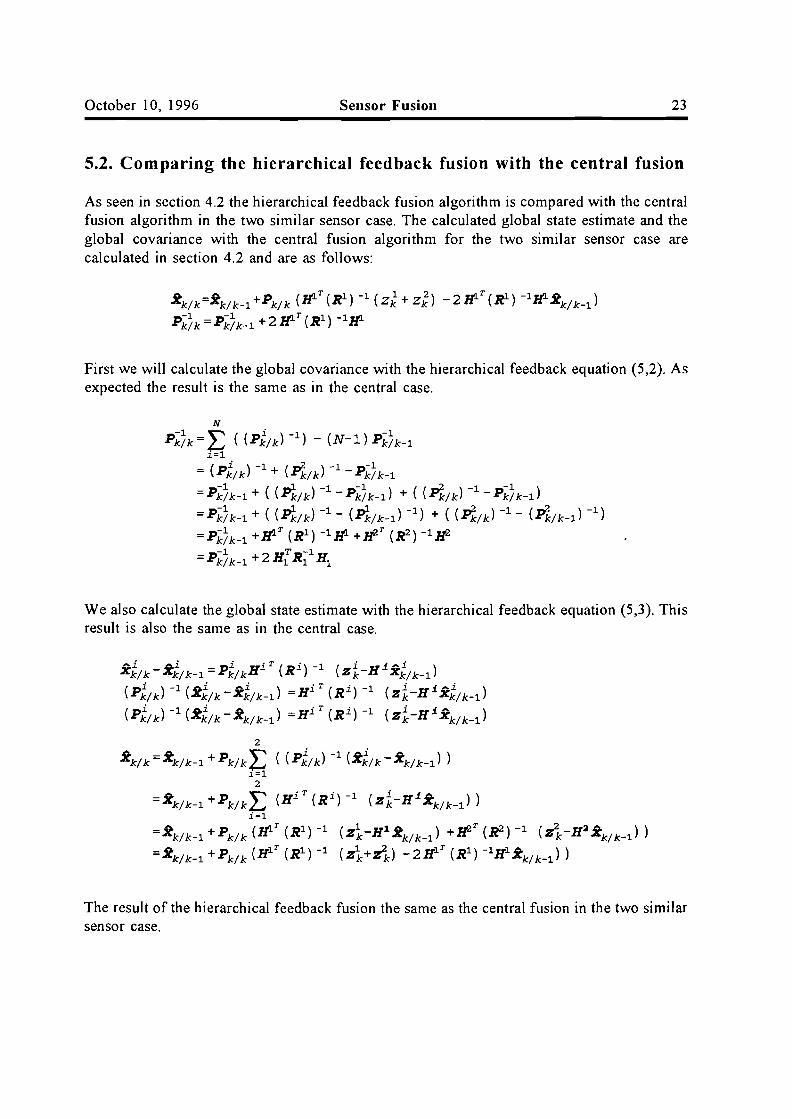
5.2. Comparing the hierarchical feedback fusion with the central fusion

As seen in section 4.2 the hierarchical feedback fusion algorithm is compared with the centralfusion algorithm in the two similar sensor case. The calculated global state estimate and theglobal covariance with the central fusion algorithm for the two similar sensor case arecalculated in section 4.2 and are as follows:

itk/k=itk/k-1 +Pk/ k (,HlT (R1) -1 (Zf + Z;) - 2,HlT (R1) -1,Hl itk/ k-1)

Pk7k=PJ::7k-1 +2,HlT(R1) -1,Hl

First we will calculate the global covariance with the hierarchical feedback equation (5,2). Asexpected the result is the same as in the central case.

We also calculate the global state estimate with the hierarchical feedback equation (5,3). Thisresult is also the same as in the central case.

2

itk/k=itk/k-1 +Pk/kL ((Pt/k) -1 (Xt/k- Xk/k-1) )i=l

2

=itk/ k-1 +Pk/kL (HiT (R i ) -1 (Z~-H1itk/k_1))i=l

=itk/ k-1+Pk/ k (,HlT (R1) -1 (Z1-H1itk/k_1) +1PT

(R2) -1 (zt-H2itk/k_1))

=itk/ k-1 +Pk/ k (H1T (R1) -1 (Z1+rk) _2H1T (R1) -lH1itk/ k_1) )

The result of the hierarchical feedback fusion the same as the central fusion in the two similarsensor case.


5.3. Reduced communication requirements

In [8, Alouani-AT] the communication requirements between central processor and localsensors is reduced. In this paper the case of two sensors is considered. In the conclusions isstated that this method can be extended to an arbitrary number of sensors. But nothing isstated, for the case with more than 2 sensors, about the expected communication requirements.Possibly only communications will be required to the first local filter and no communicationto the rest of the local filters or maybe only no communication will be required to the lastlocal filter ( local filter N) and communication to the rest of the local filters, is still necessary.

1 1 11.1 1Vk Zl Xk/k Pk/k

~5localk

filter 1A

Pk/kA

• • Xk/k ~kfusionxk• •

centerPk/k• 2 •

vk Z211.2 2

~~* local Xk/k Pk/kk

filter 2Figure 8, two sensor hierarchical fusion with reduced communication requirements

Special equations for the fusion center are derived in the two sensor case, so that if the fusedglobal state estimate and the fused global covariance is communicated to local filter 1, whichuses this information as priori statistics, and no communication is required to local filter 2,the result will be the same as with the hierarchical fusion with full feedback. The gain of thismethod is that there is no communication from the fusion centre to local filter 2, with nodegradation of performance, what is possible by the special derived equations for the fusioncenter.

The state estimate and its error covariance of sensor 2 is given by equations (5,6) and (5,7).

(5,6)

(5,7)

The predicted state estimate and the predicted covariance of sensor 2 are calculated withequation (5,8).

(5,8)


The state estimate and its error covariance of sensor 1 is given by equation (5,9) and equation(5,10).

..I .. I .J. HIT(RI)-I( I HI .. I ) (5,9)Xk/k =Xk/k-I +rk/k Zk - Xk/k-I

The predicted state estimate and the predicted covariance of sensor are calculated withequation (5,11).

Note that in equation (5,11) the predicted state estimate and the predicted covariance arecalculated with help of the previous global state estimate and global covariance of the fusionalgorithm. This is because of the feedback of the fused global state estimate and the fusedglobal covariance.

The estimates and covariances of sensor I and sensor 2 are now communicated to the centralfusion agent where they are fused to a global state estimate and global covariance, with thefusion algorithm for the two sensor case:

(5,12)

(5,13)

(5,14)

The difference with the hierarchical fusion with full feedback is in the algorithm of the fusioncenter. In the hierarchical fusion with full feedback the number of sensors is not fixed, butin the hierarchical fusion with reduced communication requirements the number of sensorsis fixed (N=2), so an extra sensor will also demand a new fusion algorithm.The is no need to connect the input Uk to the fusion center because the predicted global stateestimate can also be calculated in local filter 1 with the global state estimate that is fed back.


Chapter 6. Distributed model architecture

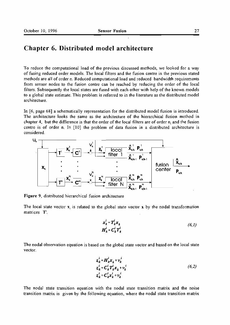
To reduce the computational load of the previous discussed methods, we looked for a wayof fusing reduced order models. The local filters and the fusion centre in the previous statedmethods are all of order n. Reduced computational load and reduced bandwidth requirementsfrom sensor nodes to the fusion centre can be reached by reducing the order of the localfilters. Subsequently the local states are fused with each other with help of the known modelsto a global state estimate. This problem is referred to in the literature as the distributed modelarchitecture.

In [6, page 68] a schematically representation for the distributed model fusion is introduced.The architecture looks the same as the architecture of the hierarchical fusion method inchapter 4, but the difference is that the order of the local filters are of order n j and the fusioncentre is of order n. In [l0] the problem of data fusion in a distributed architecture isconsidered.

Uk

Al I

local ~ Pk/k

filter 1 Al I

~-l Pk/k-l A

fusion xk/kx k

•center

Pk/kAN N

local ~ Pk/k

filter N AN N

Xk/k-l Pk/k-l

Figure 9, distributed hierarchical fusion architecture

The local state vector Xi is related to the global state vector X by the nodal transformationmatrices T.

(6,1)

The nodal observation equation is based on the global state vector and based on the local statevector.

(6,2)

The nodal state transitIOn equation with the nodal state transItion matrix and the noisetransition matrix is given by the following equation, where the nodal state transition matrix


can be obtained from the global state transition matrix using the nodal transformation matrix.

i ii ii iiXk+1=()kxk+rkwk+tkuk

()i = T~+l ()k(~.J

r~=r:+1rk(~.J

ti =T~+l t k(T~-

(6,3)

The inverse of the nodal transformation matrix is taken as the Moore-Penrose generalizedInverse.

• • T •• T

(T~) - =T~ [T~T~ ] -1

EveI)' reduced order Kalman filter has two stages, which are prediction:

(6,4)

(6,5)

and update:

(6,6)

(6,7)

The fusion equations consist of a global state estimate equation and a global covananceequation:

N

p;ixk/k =P;i-1 Xk/k-1 +L (TiT«p~.J-1X~k -(p~k_1r1x~k_1»i=l

N

p;i=p;i-1 +L (TiT«p~.J-1_(p~k_1r1)T~i=l

(6,8)

(6,9)

The predicted global estimate and the predicted global covariance can be computed from theextrapolation equations (3,6) and (3,7).Similar to the hierarchical fusion algorithm a more convenient equation for the global stateestimate is derived

I N T·· T . . (6,10)" _" p- ~ (Ti (pI )-1('" Ti" ) T i (pI )-l(Ti " _ "I »xk/k -Xk/k-1 + k/kLJ k/kJ Xk/k - Xk/k-1 + k/k-1 Xk/k-1 Xk/k-1

i=l

It can be seen that if the transformation matrix is unity, equation (6,10) is similar to thehierarchical fusion equation (4,3).


6.l.Derivation of the distributed fusion algorithm

The global and nodal noise matrices are related via:N

H TR-1H=:r; ('I'i TCi T (Ri) -1 Ci'I'i)~=1

With the help of this relation a global state covariance equation (6,9) can be derived:

Pk/k =Pk/k-1 +HTR-1HN

Pk/k =Pk/ k-1 +L ('I'i TCi T (R i ) -1 Ci 'I'i)i=l

N

Pk/k=Pk/k-1 +L ('I'iT

((Pt/k) -1_ (pf/k-1) -1) 'I'i)i=l

The global observations and the local observations are related via:N

H TR-1Zk =:r; ('I'i TCi T (R i ) -1 zt)~=1

With help of this relation a global state estimate equation (6,8) can be derived:,.-i _ ... i pi Ci T (Ri ) -1 ( i C 1 Ai )Xk/k-Xk/k-1 + k/k Zk- A.k/k-1(pi )-l(Ai Ai ) CiT(Ri)-lC1Ai CiT (R i )-l ik/k A.k/k - A.k/k-1 + A.k/k-1 = Z k

(Pt/k) -lSCt/k+ (Ci T (R i ) -lC 1 - (pf/k) -1)SCf/k_1 =CiT (R i ) -l z t(pi ) -lAi (pi ) -lAi Ci T (R i ) -1 ik/ k A.k/k - k/k-1 A.k/k-1 = . Z k

N

HTR-1 ~ 'I'i T((pi ) -lAi (pi ) -l Ai )Zk=~ k/k A.k/k- k/k-1 Ak/k-1~=1

With the rewritten equation (3,4) put in the equation above, we get an equation for the globalstate estimate.

itk/k=itk/k-1 +Pk/ k H TR-1 (zk -Hitk/ k-1 )

Pk/kitk/k=Pk/kitk/k-1 + H TR-1 (zk -Hitk/ k-1 )

= (Pk/ k -1 +HTR-1H) itk/ k -1+HTR-1Zk-HTR-1Hitk/k_1_ -1 A T -1-Pk/ k-1A.k/k-1 +H R Zk

N

=Pk/k-1 itk/ k-1 +L ('I'i T( (pf/k) -liCf/k- (Pt/k-1) -liCf/k_1) )i=l


Now with help of equations (6,8) and (6,9) a more convenient equation for the global stateestimate is derived,

N

Pl/ik=Pk/k-1 +~ (TiT ((Pt/k) -1_ (Pt/k-1) -1) T i )~=1

N-1 A -1.... ~ (Ti T (pi ) -1 T i A Ti T (pi ) -1 T i A )

Pk/k Ak/k-1 =Pk/k-1Xk/k-1 + L k/k A k/k-1 - k/k-1 Ak/k-1i=l

N-1.... -1 .... ~ (T;T(pi )-IT;A TiT(pi )-IT;A )

Pk/k-1 X k/ k-1 = Pk/kXk/k-1 - L ~ k/k ~ Ak/k-1 - k/k-1 ~ Ak/k-1i=l

N

P -1 A -1 A ~ (Ti T (pi ) -lAi T i T (pi ) -l A i )k/kAk/k =Pk/k-1Ak/k-1 + L k/k Ak/k- k/k-1 Ak/k-1

i=lN

-1 A -1 .... ~ (Ti T (pi ) -1 Ti A T i T (pi ) -1 T i A )Pk/kAk/k =Pk/kXk/k-1 - L k/k A k/ k-1 - k/k-1 Ak/ k-1 +

i=lN

" (Ti T (Pt/k) -lRi/k- T i T (pi/k-l) -lRt/k_1)+f;fX k/ k = Rk/ k -1 +

N

+Pk/k~ (TiT (Pt/k) -1 (ftt/k-TiXk/k_1) +TiT

(Pt/k-1) -1 (Ti ftk/ k _1 -Ri/k-1))~=1

So in this section the fusion equations (6,8), (6,9) and (6,10), for the distributed modelarchitecture that is represented in chapter 6, are derived.


Chapter 7. Hoo filtering

The aim of this section is define an estimator, dual to the Kalman filters in the previouschapters, that takes into account the frequency dependent properties of a sensor. Such kindof estimator is found in the Hoo filter. So we try to find a way of designing a Hoo filter thattakes into account the frequency dependent properties of a sensor. We are looking for a wayto define a Hoo filter in similar way the central filter (chapter 3) is defined for fusingmeasurement data.

We looked in the literature if Hoo filtering was used in combination with sensor fusion, butno efforts in that direction were found.

Just like the Kalman filter, The Hoo filter is a causal, linear mapping taking the control inputu and the measurement y as its inputs, and producing an estimate 2 of the signal z in suchway that the Hoo norm of the transfer function from the noise w to the estimation error e=z-2is minimal. We want to design a filter mapping (u,y)~2 such that the for overall configurationwith transfer function E:(w,v)~e the Hoo norm is less than or equal to some pre-specifiedvalue l. In this way the Hoc, filter is defined, we need access to the input u.

We consider the state space equations:

i =Ax +B)w +B2uz=C)x+D2 )u

Y =CzX+v

(7,1)

The Hoo norm is defined by:

2Ileib2 2Ilwlb + Ilvlb

(7,2)

The configuration of the Hoo is:

1\Z

)-----. ez-- ~plant

<:r!--1.----.. Hinf filter -

iv

w

u

Figure 10, The Hoo filter configuration


The solution to this problem is given by the following theorem:Theorem of the H oo filter:There exists a filter which achieves that the mapping E:(w,v)--,;e in the configuration ofFigure 10 satisfies

IIEII"" <y

if the following Riccati equation has a stabilizing solution y= yT~O.

O=AY + YA T - Y[C2TC

2-y-2CtCI]Y+BIBt

In that case one such filter is given by the equation

. 2 T~ =(A+y- BIBI X)~ +B2u+L(C2~-Y)

Z=CI~ +D21u

L=YC;

For the Roo we assume that the following assumptions hold:A-I D ll = 0 and D22 = O.A-2 The triple (A, B 2, C2) is stabilizable and detectable.A-3 The triple (A, B l , C l ) is stabilizable and detectable.A-4 DT

I2 (C l D 12 ) = (0 I).A-5 D\I (BTl D\l) = (0 I).

(7,3)

(7,4)

Assumption A-I states that there is no direct feedthrough in the transfers w --'; z and u --'; z.The second assumption A-2 states that internally stabilizing controllers exist. AssumptionA-3 is a technical assumption made on the transfer function. Assumptions A-4 and A-5 arejust scaling assumptions that can be easily removed. Further explanation on the assumptionscan be found [11, page 64].

The resulting filter is a filter like the Kalman filter but the difference is that there is no realcovariance estimated, but the resulting matrix L (the H oo filter gain) depends on the value ofy and y depends on Y.

The computation of H,,, filters can be done with the various routines included in the MatlabRobust Control Toolbox. For the Roo filter design is of importance the Matlab routine hinfand the time discrete variant dhinf.

For the time discrete domain we consider the state space equations:

Xk+1 =Axk +BI wk +B2uk

Zk=CIXk +D12 uk

Yk=C2X k +vk

(7,5)


We define Yk , C2 and V k equal to the difinition in chapter 3 to allow several sensormeasurements into the system.

I)T N)T- TYk Gt. [(Yk , •••• , (Yk ]

Cz Gt.[(C~l , .... , (C:)7]T

Vk Gt. [(Vi)T , •... , (vtlf

This is equal to:

(7,6)

(7,7)

The discrete time R"" filter is now configured by:

Wk

Uk ~x.c C1

Z+ Z .- + e

LG= YkC21\

+ zHinf filter

~vk

L

Figure 11, The discrete time Roo filter configuration

With this definitions it must can construct a filter with a structure that looks like the centralfusion structure. The construction of the Roo filter is not carried out yet because we want firstlook to the simulation results of the previous found fusion algorithms.

October 10, 1996

Chapter 8. Sim ulations

Sensor Fusion 35

In this chapter we carry out simulations with the various fusion algorithms on a simple modelwith inputs vectors and noise vectors generated by matlab. The reason for using datagenerated by matlab is that it is easier to compare the fusion algorithms. We want toinvestigate the effect of various sensor measurements and sensor noises on the fusionalgorithms. We are also interested in the effect of bias in a sensor measurement and thepossibility of detecting a defect or inaccurate sensor.

8.1. Simulation model

The model used is a vehicle moving in one direction, namely position x. The input vectorsof the model are the control input u and the process noise w.

u-------.·I/LJG~w_______.. ID ~OJ

position x~

Figure 12, vehicle

The state vector is assumed to consist of position and velocity.

(8,1)

The control input u and the process noise ware entered in the system as an acceleration a.where the a is the damping of the system, in our simulations equal to zero.

(8,2)

Measuring the position x is done by:

(8,3)

Measuring the speed v is done by:

(8,4)

Because all the fusion algorithms are derived for the discrete time the model is converted to


a discrete time model. This conversion is performed with the matlab conversion programC2DM, which converts the continuous time state-space system to a discrete time state-spacesystem. The conversion method used is a zero order hold. The discrete time state spacesystem is now defined.by ( in this case the damping a. is equal to zero):

(8,5)

Where T is the sampling period.The measurement equations for measuring the position and the speed are the same as in thetime continuous case with as only difference the time indices k.

position measurement:

(8,6)

speed measurement:

(8,7)

First we make a matlab file (Appendix B: makedat.m) that produces measurement data of theposition and the speed and also some sensor noise and with process error. Assumed is thatthe initial state at t=O is known, the position and speed at t=O are equal to zero.

, 0

10

j

t ( 5 ec )

j

t ( 5 ec )

a 0

E 6 0

": ~ 0

::: I 0~

00

40

-E

"-~.-o·~ 10:"

4 00

Figure 13, Position arid speed of vehicle

From t=O sec to the input u is a constant acceleration of 10 mis, then the acceleration is zerofor 2 seconds, then the acceleration is -20 mls for 2 seconds next the acceleration is zero for2 seconds and the last 2 seconds the acceleration is 10 m/s. The sampling time T=0.2 sec isequal to 10 sec divided by the amount of samples (l0 sec I 500 = 0.02 sec).


The syntax for makedat.m is makedat(samples,Q,RI ,R2,R3,R4), where samples is the amountof samples taken, Q is the process noise variance and Rl through R4 the variances of foursensor noises which can be added on a position or speed measurement. The m-file makedat.mreturns a vector that consists of a position (measure(:,l» and a speed measurement(measure(2,:) without noise and 4 independent sensor noises with variances given at the inputof the m-file. The shape of the return vector is [measure, nl, n2, n3, n4, A, B, C, Q, u]. Them-file resets the seed of the random generation every time it is used, because of this therandom noise generators (RANDN) will give the same result and so will not influence theresult of the different fusion algorithms.

We made Figure 13 with 500 samples, a process noise variance of 0.1. In the figure theposition and the speed are represented without the sensor noise added. Because of this setupwe make position and speed measurements by adding sensor noise (nl to n2) to theobservation.

The syntax in the matlab command window is:»[measure,n 1,n2,n3,n4,A,B,C,Q,u] = makedat(500,0.1, 1,1,1,1);

The mean values and variances of the returned noises are:» mean(nl)= -0.0779 var(nl) = 1.1028» mean(n2)= -0.0174 var(n2) = 1.0272»mean(n3)= 0.0058 var(n3) = 1.0020» mean(n4)= -0.0112 var(n4) = 1.1010

As seen the mean value of the returned noises are not completely zero and the variancesdiffer a little from each other and the value at the input. This is caused by the finite lengthof the noise vector, namely 500 samples.

8.2. Two position sensors

In this section we compare the result of the fusion algorithms when we have two positionmeasurements. The measurement equations of the two sensors are given by:

Z~=[1 O]Xk+V;

z~= [1 0] x k +V;(8,8)

With the measurement data generated in section 8.1 we can define the two measurementvectors Zl and Z2 by adding two uncorrelated noises (e.g. nl and n2) on the positionmeasurement vector measure(:,l). With the resulting measurement vectors Zl = (position +n 1) and Z2 = (position + n2) we investigate the result of the different fusion algorithms.

First we looked what happens in the 2 position measurements are added and divided by 2.The error n of the fused signal can be calculate with n = ( Zl + Z2 )/2 - measure(:,l). Wheremeasure(:,l) represents the original position vector, not corrupted with noise.


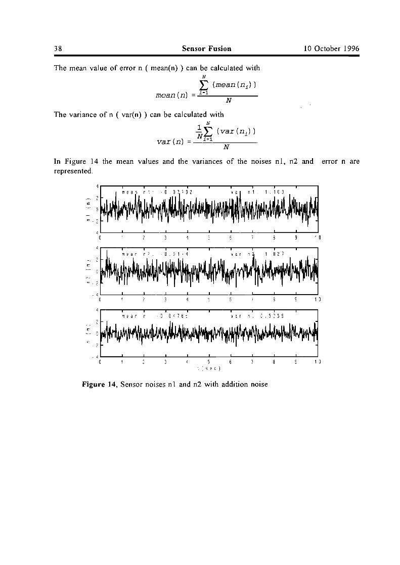
The mean value of error n ( mean(n) ) can be calculated withN

~ (mean (nJ)mean (n) = ----:-::---

N

The variance of n ( var(n) ) can be calculated withN

.!L (var (ni) )

()Ni=lvar n = -...::.....::------

N

In Figure 14 the mean values and the variances of the nOIses nl, n2 and error n arerepresented.

c _ 2

1 0

E

4L...-_---L__....L...__.1...-_----1.__....L..__.1.-_----1__----1....__...L.-_----l

o

mean n2 -0.0174 v a r n 1 0 2 7

E

c _ 2

1 0

4'--_--L__-'-__.L.-_--l.__-'-__-'--_--'-__--'-__...L.-_----'

I]

mean n -004755 var n. 0,5259

1 05t ( 5 e c )

- 4 '--_--L__-'-__.L.-_--l.__-'-__-'--_--'-__--'-__...L.-_----'

o

Figure 14, Sensor noises nl and n2 with addition noise


We also looked with matlab to the behaviour of the variance of error n as a function of theproportion of the variance of n1 and the variance of n2. The variance of n1 is set to 1 andthe variance of n2 is calculated with a proportion V=var(n2)/var(nl) vary from 1 to 10.

;'.5

',5

, 5 6 1II r GflO r I I I) n '!f (II:.' ) I Wll f (II 1)

a 5 '------'-_---'-_--'-_-'-----_'-------'-_----'-_---'------J,

Figure 15, variance n versus proportion V

In Figure 15 is expressed that if the variance of n2 more than 3 times the variance of n1 theresulting error variance becomes bigger than the noise variance of n1, so if one only looksat the variance there is no profit in that case.


8.2.1. Central fusion with 2 position sensors

In this section we investigate the result when the two position measurements Zl and Z2 arefused with the central fusion method. The equations of the central fusion algorithm are placedin the matlab file central.m and this file is used in the matlab file centr82.m to produce thesimulation results that can be compared with the results of the measurement addition in theprevious section and the fusion algorithm in the next section. Both the matlab files central.mand centr82.m are presented in appendix C. In Figure 16 the position error after fusing Zl andZ2 is displayed, the mean value and the variance are calculated after 2 seconds when thecovariance matrix Pglob almost reached his final value.

1 05Irs e c )

- 0 J '-_...I.-_--'-_---L._----J'-_...L-_--'--_----'-_----J'---_-'--_--'o

_ D 1

- 0 2

E

D I

D , 2 .------r---r------.------,.------.------,-----r------,.------.-----,

o , I ,-----r---r------.------,.------.------,-----r------,.------.-----,

o D8

:: D D6

;:;:- 0 , D4

o 0 2

1 05I ( 5 e c )

o '-_...I.-_--'-_---L._----J'---_...L-_--'--_----'-_----J__-'--_--'o

Figure 16, Central fusion with 2 position measurements

You can see that the mean(noise)=-0.07667, this value is larger than the mean value aftersimple measurement addition (-0.04766). The variance (var(noise)=0.001183) is much smallerthan the variance after simple measurement addition (0.5259), this effect is also due toaveraging the measurements over more samples. So one can not compare this two results witheach other.

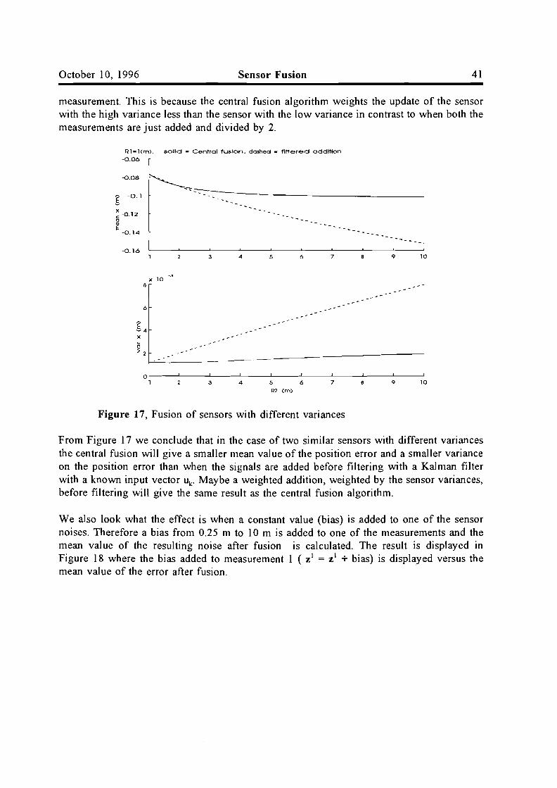
Now we investigate what the effect is when the variances of the sensor noises are different.The variance R2 was increased from 1 to 10 and the variance Rl hold to 1. The mean andvariance were compared to the mean and variance of a filtered addition measurement, theresults are represented in Figure 17. We found that the mean and the variance of the errorwith the central fusion increased less than the mean and variance of the filtered addition


measurement. This is because the central fusion algorithm weights the update of the sensorwith the high variance less than the sensor with the low variance in contrast to when both themeasurements are just added and divided by 2.

Figure 17, Fusion of sensors with different variances

From Figure 17 we conclude that in the case of two similar sensors with different variancesthe central fusion will give a smaller mean value of the position error and a smaller varianceon the position error than when the signals are added before filtering with a Kalman filterwith a known input vector Uk. Maybe a weighted addition, weighted by the sensor variances,before filtering will give the same result as the central fusion algorithm.

We also look what the effect is when a constant value (bias) is added to one of the sensornoises. Therefore a bias from 0.25 m to 10m is added to one of the measurements and themean value of the resulting noise after fusion is calculated. The result is displayed inFigure 18 where the bias added to measurement 1 ( Zl = Zl + bias) is displayed versus themean value of the error after fusion.


'0j

bias (III)

o'-----'-_-'-------'-_---'---_L-------'-_--'-------'-_---'---_o

Figure 18, Bias versus mean(noise)

Half the bias added to a measurement returns in the mean value of the noise after the centralfusion. This is the same result as if the two measurements are simply added and divided by2.

The same simulations done with the central fusion algorithm and two position sensors areperformed with the other fusion algorithms, namely:

-Hierarchical fusion with two position sensors. (Appendix D)-Hierarchical fusion with feedback and two position sensors. (Appendix E)-hierarchical fusion with reduced feedback and two position sensors. (Appendix F)

The results of these simulations are exactly the same as the fusion with the central fusionalgorithm. Therefore this results are not represented in this report. At this moment thedifferent fusion algorithms show no difference in the resulting state vectors with differentnoise variances and different biasses. Therefore we look in the next section how the differentfusion algorithm respond to one position measurement and one speed measurement.


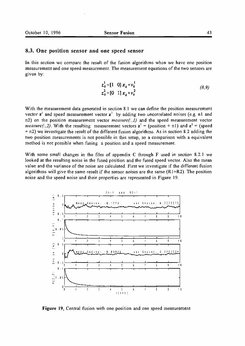
8.3. One position sensor and one speed sensor

In this section we compare the result of the fusion algorithms when we have one positionmeasurement and one speed measurement. The measurement equations of the two sensors aregiven by:

(8,9)

With the measurement data generated in section 8.1 we can define the position measurementvector Zl and speed measurement vector z~ by adding two uncorrelated noises (e.g. nl andn2) on the position measurement vector measure(, 1) and the speed measurement vectormeasure(,2). With the resulting measurement vectors Zl = (position + nl) and Z2 = (speed+ n2) we investigate the result of the different fusion algorithms. As in section 8.2 adding thetwo position measurements is not possible in this setup, so a comparison with a equivalentmethod is not possible when fusing a position and a speed measurement.

With some small changes in the files of appendix C through F used in section 8.2.1 welooked at the resulting noise in the fused position and the fused speed vector. Also the meanvalue and the variance of the noise are calculated. First we investigate if the different fusionalgorithms will give the same result if the sensor noises are the same (R 1=R2). The positionnoise and the speed noise and their properties are represented in Figure 19.

Rlo1 and R2o!

E°. 5 r---,---,---r---r---,---r---r---,-----,.-----,

-°. ! 2 2 8 ,ar Xnolse. 0.0009015

:: -° 5 '--_-L-_---'-__L-_-L-_---'-__L-_....I...-_---'-__L---l

° 2 3 5 1°

_:};: : : : : : : : : ]° 1 °-- ° 5 r---,---,---.----r---,---.----r---,---.-----,

E

° rf'""m""e".a,rD.."",-s...n ....0 ,..:.1s~e",:_ . .;...0....0;.;3:,.;9,..2...6--..__' a;..r-::s.....n.;.o_I;...Se__. .....0_...:.,0;-0....0 _72;....3'-14

~ -°.5 '--_-L-_---'-__L-_....I...-_---'-__L-_....I...-_---'-__L...---l

° 2 3 5 6 8 10

~,'':K:: : : : : : : : ]° I 5 B 1°

I ( sec )

Figure 19, Central fusion with one position and one speed measurement


The simulation of Figure 19 is performed with the central fusion algorithm, the samesimulations were performed with the hierarchical fusion, hierarchical fusion with feedback andthe hierarchical fusion with reduced feedback fusion algorithms. They all show in the caseof Rl =R2 exactly the same result.

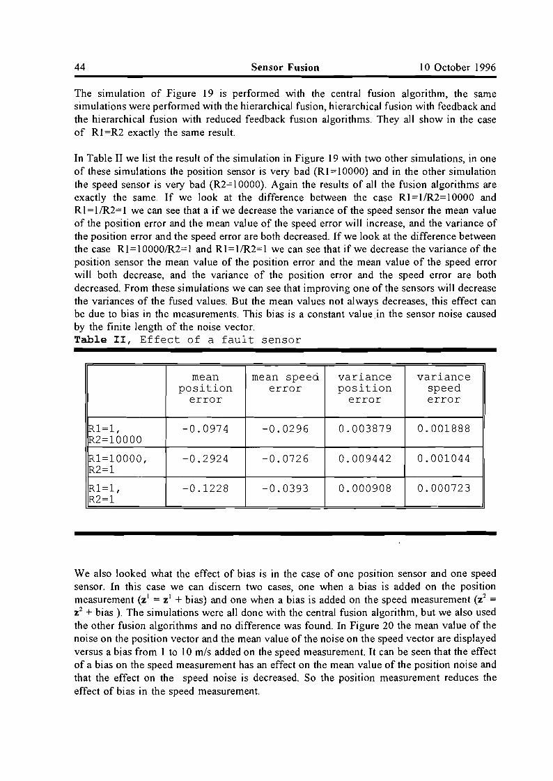
In Table II we list the result of the simulation in Figure 19 with two other simulations, in oneof these simulations the position sensor is very bad (Rl = 10000) and in the other simulationthe speed sensor is very bad (R2= 10000). Again the results of all the fusion algorithms areexactly the same. If we look at the difference between the case Rl=IIR2=10000 andRI=11R2=1 we can see that a if we decrease the variance of the speed sensor the mean valueof the position error and the mean value of the speed error will increase, and the variance ofthe position error and the speed error are both decreased. If we look at the difference betweenthe case Rl=100001R2=1 and Rl=11R2=1 we can see that if we decrease the variance of theposition sensor the mean value of the position error and the mean value of the speed errorwill both decrease, and the variance of the position error and the speed error are bothdecreased. From these simulations we can see that improving one of the sensors will decreasethe variances of the fused values. But the mean values not always decreases, this effect canbe due to bias in the measurements. This bias is a constant val ue.in the sensor noise causedby the finite length of the noise vector.Table II, Effect of a fault sensor

mean mean speed variance varianceposition error position speed

error error error

R1=1, -0.0974 -0.0296 0.003879 0.001888R2=10000

R1=10000, -0.2924 -0.0726 0.009442 0.001044R2=1

R1=1, -0.1228 -0.0393 0.000908 0.000723R2=1

We also looked what the effect of bias is in the case of one position sensor and one speedsensor. In this case we can discern two cases, one when a bias is added on the positionmeasurement (Zl = Z' + bias) and one when a bias is added on the speed measurement (Z2 =Z2 + bias ). The simulations were all done with the central fusion algorithm, but we also usedthe other fusion algorithms and no difference was found. In Figure 20 the mean value of thenoise on the position vector and the mean value of the noise on the speed vector are displayedversus a bias from 1 to 10 mls added on the speed measurement. It can be seen that the effectof a bias on the speed measurement has an effect on the mean value of the position noise andthat the effect on the speed noise is decreased. So the position measurement reduces theeffect of bias in the speed measurement.


R , = 1 ~ n d R ? = 1E- a.------r--.....,....----.--r---r----,------,.------r----,

10

::: i r---r--.....,....----.--r---r----,------,.------r----,E

cno L..-_....I..-_--L.._----'__.L--_........._---'-_----JL...-_...L..-_--'~ I i \ 6 7 a 10

bl~s on speed measurement [m/s)

Figure 20, Bias on the speed measurement

In Figure 21 the mean value of the position error and the mean value of the speed error aredisplayed versus a bias from 1 to 10 m/s added on the position measurement. It can be seenthat the bias on the position measurement completely returns in the mean value of the positionerror. So the mean value of position error is not decreased by the speed measurement. Thissounds logic, because the speed is the derivative of the position and so has no informationabout a constand value in the position measurement.

10

J i I 6 7 RIOb i a SOft P 0 5 I t I (I ft II t a 5 u r ell e n t (II)

-~_1 0

-"'-..c~

- i

~

~

c0n

1~

- 0 II

~0 I

- 0 .0\..~

=:~-cn 0 . 0 \.. 1~

Figure 21, Bias on the position measurement


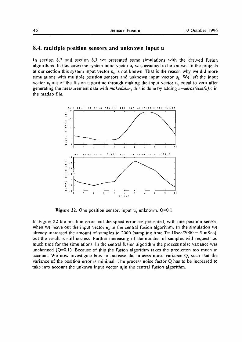
8.4. multiple position sensors and unknown input u

In section 8.2 and section 8.3 we presented some simulations with the derived fusionalgorithms. In this cases the system input vector Uk was assumed to be known. In the projectsat our section this system input vector Uk is not known. That is the reason why we did moresimulations with multiple position sensors and unknown input vector Uk' We left the inputvector Uk out of the fusion algoritme through making the input vector Uk equal to zero aftergenerating the measurement data with makedat.m, this is done by adding u=zeros(size(u)); inthe matlab file.

medn position error =10.SS dnd ~(Ir position error =69.51J 0 .-----r--.,....---r----.-----r----.---~----.--___,_-___,

E

_ 20

medn speed error =B.~BS I'nd Vdr speed error ::196.840

- J 0

20

- 10

::: -, 0~

if' . 1 0 '---_.1..-_..I--_...L-_-'---_--L.-_--'--_--'-_--'-_---L_----'o \ 1 0

t ( 50 C ]

Figu.oe 22, One position sensor, input Uk unknown, Q==O.1

In Figure 22 the position error and the speed error are presented, with one position sensor,when we leave out the input vector Uk in the central fusion algorithm. In the simulation wealready increased the amount of samples to 2000 (sampling time T== 10sec/2000 == 5 mSec),but the result is still useless. Further increasing of the number of samples will request toomuch time for the simulations. In the central fusion algorithm the process noise variance wasunchanged (Q==O.I). Because of this the fusion algorithm takes the prediction too much inaccount. We now investigate how to increase the process noise variance Q, such that thevariance of the position error is minimal. The process noise factor Q has to be increased totake into account the unkown input vector ukin the central fusion algorithm.

October 10, 1996 Sensor Fusion

o 2 .------r---.---.----r-----r--.------r--...,.--.....---,

\0,18

E

- 0, 16

:::0,11

:':0,12

0,1

o 0 8 L----..JL....-----..JL....-----..J_:::::=:::::i=:::::::::;:==::::::l==::::::l=:::::::l==:::::lo 0 , 2 0 4 0 , 6 0 8 1 1 , 2 1 4 1. 6 1 , B 2

oro Ce s s no i seQ ~ 1 at

47

Figure 23, Variance position errror versus process noise Q

From Figure 23 we can determine the Q==14000 that will give a minimum variance on theposition error. This value doesn't have to bee exact 14000, and also depends on the used inputvector u. Now we do the same simulation as in Figure 22 with the same number of samples(samples == 2000), one position sensor but the process noise Q==14000. In the resultingFigure 24 we see that the resulting position error is improved by increasing the process noiseQ in the central fusion algorithm

mean position error =0.0066J9 and war pasilloll error =O,08?~

1 , 5 ...-----r--...,.--.....---,---r-----r----,.....--r---r----,

mean speed error =0,7721 and war speed error =i.S185 0 ...-----r--...,.--.....---,---r-----r----.,.....--r---r----,

E0".- -- ~

50-w~

I 0 0ww~

~

~ 1500 5 10

t I "t I

Figure 24, One position sensor, input Uk unknown, Q==14000

Now we have found how we can reach a minimum variance of the position error, we look if


we can improve this result by adding more position sensors. Simulations were performed withN=l to N=8 position sensors, and of each simulation the calculated mean value and varianceof the position error and the speed error are presented in table Table III.

Table III, Effect of N position sensors on error

N mean pOSe variance mean speed var.speederror pOSe error error error

1 0.00668 0.0825 0.2724 4.548

2 -0.01573 0.0400 0.2161 3.319

3 0.01187 0.0235 0.2143 2.633

4 -0.00016 0.0214 0.2101 2.619

5 0.00002 0.0166 0.2101 2.396

6 0.00175 0.0137 0.2011 2.141

7 0.00136 0.0119 0.1939 2.027

8 0.00237 0.0114 0.1807 2.049

The simulation of eight position sensors is performed again, equivalent to Figure' 23, toinvestigate if the used process noise Q=14000 will give the minimum variance on the positionerror.

0.019

0 018

-;0 a I}

-~

00 016

-..- 0 01 j

::0 0110~

:':0 .01 J~

~

:;;0 . c , }-C. 0 11

0.010 o.} O.~ 06 0.8 1 I.} I.~ 1.6 1.8 }

DrOCf5S nOise a I 10 4

Figure 25, Variance position error versus process noise Q, withN=8


4N position sensors

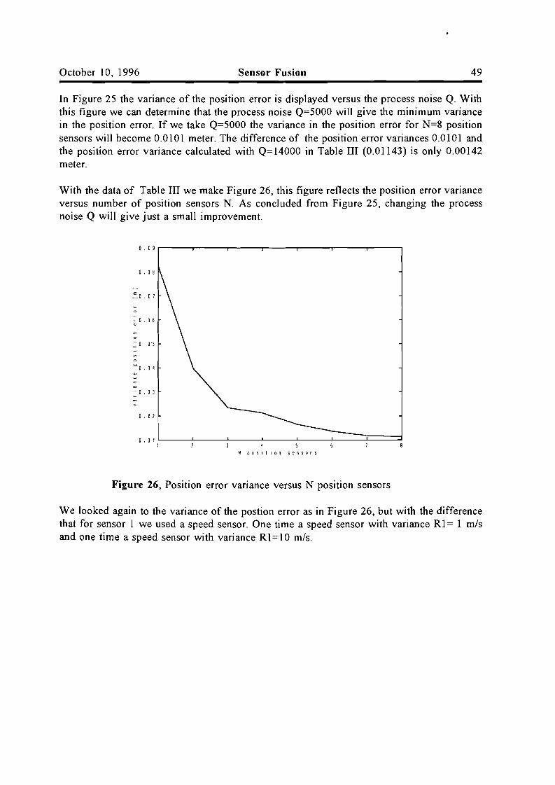
In Figure 25 the variance of the position error is displayed versus the process noise Q. Withthis figure we can determine that the process noise Q==5000 will give the minimum variancein the position error. If we take Q=5000 the variance in the position error for N=8 positionsensors will become 0.0101 meter. The difference of the position error variances 0.0101 andthe position error variance calculated with Q=14000 in Table III (0.01143) is only 0.00142meter.

With the data of Table III we make Figure 26, this figure reflects the position error varianceversus number of position sensors N. As concluded from Figure 25, changing the processnoise Q will give just a sma)) improvement.

o , 0 9 ,----,-------,...-------,.-------,-----,-----,-----,

0,0 B

-=- 0 , 0 I

=: 0 O'S

~

0

=0 04~

~

~

~

- 0 0 3~

>

o . 0 2

o , 0 1 L_----'__.......J..__---'-__....1.-__-=====:r::::=:~1

Figure 26, Position error variance versus N position sensors

We looked again to the variance of the postion error as in Figure 26, but with the differencethat for sensor I we used a speed sensor. One time a speed sensor with variance Rl == 1 mlsand one time a speed sensor with variance RI==IO m/s.


0.09 r

0.08

0.07

0.06

g~ 0.05gGIC 0.040E00. 0.03G>Uc.Q(; 0.02>

0.01

'- -- ------764 53

0'-----'--------'----'-·_.----'-J.,--,-'---,',---"-' "---'-'-'.'--,---"--"-'..L','-----"----'--"-------',_''-----"----'--"--J.,1

N position sensors

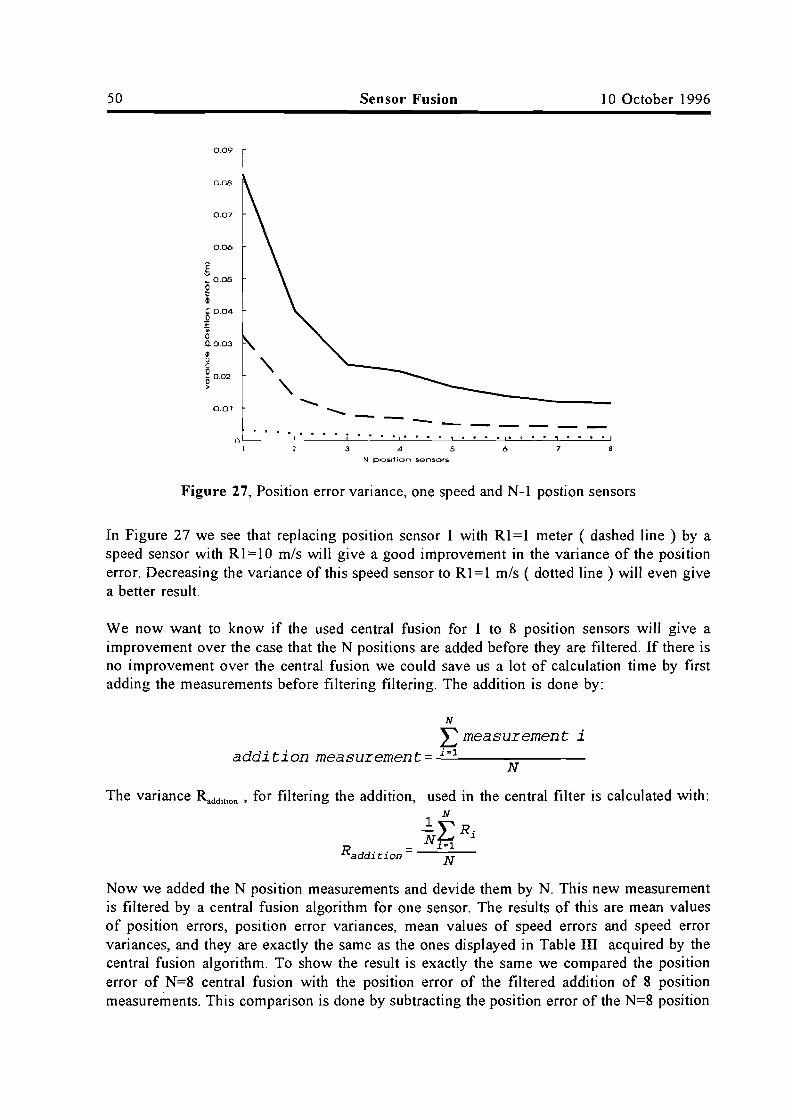
Figure 27, Position error variance, one speed and N-l postion sensors

In Figure 27 we see that replacing position sensor 1 with Rl = 1 meter ( dashed line) by aspeed sensor with Rl=10 m/s will give a good improvement in the variance of the positionerror. Decreasing the variance of this speed sensor to R1=1 m/s ( dotted line) will even givea better result.

We now want to know if the used central fusion for 1 to 8 posItIOn sensors will give aimprovement over the case that the N positions are added before they are filtered. If there isno improvement over the central fusion we could save us a lot of calculation time by firstadding the measurements before filtering filtering. The addition is done by:

N

L measurement iaddition measurement=-i-:-l--------

N

The variance Raddition , for filtering the addition, used in the central filter is calculated with:1 N-LRi_ N i : 1

Raddition - N

Now we added the N position measurements and devide them by N. This new measurementis filtered by a central fusion algorithm for one sensor. The results of this are mean valuesof position errors, position error variances, mean values of speed errors and speed errorvariances, and they are exactly the same as the ones displayed in Table III acquired by thecentral fusion algorithm. To show the result is exactly the same we compared the positionerror of N=8 central fusion with the position error of the filtered addition of 8 positionmeasurements. This comparison is done by subtracting the position error of the N=8 position


sensor central fusion result from the N=8 position measurements added before filtering. InFigure 28 we can see that the difference is maximal 5* 10. 14

, so this is almost zero exept asmall error due to computer calculation accuracy.

E N:8 position sensors central fusion

~::~o 1 2 ] ~ l 6 7 B 9 10

:[ N=B position measurements added before filtering

o::~o I 2 J ~ l 6 ) B 9 I 0

:~r':~: jo 2 1 ~ l 6 ] B 1 0

t (s e c )

Figure 28, Difference central fusion and filtered addition, N=8

So we can save a lot of calculation time if we just add the N position measurements, withequal variances, before filtering. This is in the special case that all the sensor noise variancesare exactly the same, Figure 17 already showed that if the sensor variances are different thecentral fusion algorithm gives a lower variance on the position error.


In Figure 29, we compare the position error with N=8 posItIOn sensors fused with centralfusion algorithm and fused hierarchical fusion algorithm. Again there very small differencecaused by calculation accuracy. The strange schape of the difference can be explained by thelooking at the shape of position x in Figure 13. If the x becomes larger the calculation errorsalso grow.

~ N = 8 pas i tIll n 5 ens 0 r 5 tell t I B I I U 5 Ion

:::~- 0 1 2 3 ~ j 6 ) B 9 10e N: B hie fIr c b I Ca I r us i 01\

<::~~o 1 2 3 ~ 5 6 1 B 9 1 0

o·r':~:j= 0 2 3 ~ 5 6 1 B 9 10

t (sec)

Figure 29, Difference central fusion with hierarchicalfusion for N=8

In Figure 32 we investigate the difference between the central fusion and the hierarchicalfusion with feedback. Again the result of both the fusion algorithms is the same.

~ N: B po 5 I [ ion 5 ens 0 r 5 c e nt' s I Ius jon

<::~- 0 1 2 J ~ j 6 ) B 9 10!. N=8 Rlerarchlcal fUSll1n _It" feedback

<::~o I 2 l ~ 5 6 7 B g 1 0

: .5

5

:' 10'" differ"" bel."" pOSlli" erl""

.- . 0

·1o I 2 l ~ 5 6 7 B 9 1 0

I (s,,)

Figure 30, Difference central fusion with hierarchicalfusion with feedbak for N=8 position sensors.


8.5. Detecting a fault sensor

In this section we investigate if it is possible to detect, with help of the global measurementand a sensor measurement, a fault sensor. In Figure 31 we show how a error signal with theglobal state estimate and the sensor measurement is defined in the central fusion scheme.

~Pk/k

central Afusion Xwk

~N

Uk ---------1---------;

Vk

+ HI

r +HN(r-•

el

I I I eN

Figure 31, Error signal definition for fault sensor detection

The error signal ei is defined by:

(8,10)

We now do a simulation with the same one dimensional dynamic model as used in the othersections, with unknown input vector Uk , three position sensors and 2000 samples (T=10 sec12000 samples = 5 mSec). We will disrupt one of the position measurements with noise andbias, whereafter we look at the effect on the error signal ei

. In Figure 32 the error signal thatis added on the position measurement of sensor 2 is displayed, also the three correspondingerror signals according to equation (8,10) are displayed. The error signal is a constand value(bias) of 10 meter added from t=2 to t=4 seconds, and a zero mean noise with variance R=4meter added from t=6 to t=4 seconds.

54 Sensor Fusion

error signal on posltl()n measurement 2

o J------r-:! : ! : ~ : Io 1 2 3 4 5 6 7 B 9 1 0

<~o 1 2 J 4 5 6 ) B 9 1 0

::~~~.~~~~o 1 1 J 4 5 6 7 B 9 1 0

~,i~o 1 2 J 4 5 6 1 B 9 1 0

Figure 32, Error signals of three position measurements

10 October 1996

It can be seen from the figure that the bias on position measurement 2 has infuence on allthree the error signals. But the effect is larger in the error signal of measurement 2 than onthe other measurements. The zero mean white noise is also visible in the error signal ofposition measurement 2. From Figure 32 can be seen that the effect extra bias or extra noiseon a sensor measurement can be detected from the defined error signal. To do a correct faultsensor detection, a norm for this has to be defined.

October 10, 1996

Chapter 9. Conclusions

Sensor Fusion 55

A simple way in fusing sensor measurements is found in the central fusion architecture. If thesensors process their data locally, and sending their estimates to a central processor,alternative fusing algorithms are needed. A solution for this is found in hierarchical fusionalgorithm. The hierarchical fusion algorithm is compared algebraical to the central fusionarchitecture in the two similar sensor case, which yields the same results. In the litarature wasstated that an advantage of the hierarchical fusion algorithms is that it is easy to detect sensorfailure by comparing the local estimate with the global estimate. This is not completelycorrect, because with a defined error signal e, it must also be possible to detect a fault sensorin the central fusion case. A disadvantage is the growing computational load, because thesame system model as the central fusion node is used in every local node.The global state estimate in the hierarchical architecture can also be fed back to the localnodes to be used as priori statistics. This method is also compared algebraical to the centralfusion architecture in the two similar sensor case, which yields the same results. The feedbackof the globel state estimate and the global covariance yields extra communicationrequirements, these communication can by reduced by using the algorithm derived in [8,Alouani-AT]. This algorithm is only derived for the 2 sensor case. The hierarchicalarchitectures with and without feedback are both derived from the central architecture. Theyare also both compared algebraical with the central architecture in the two similar sensor case,from which we conclude that in this case the result of the three architectures are the same.

Because of the growing computational load with hierarchical fusion algorithm we looked fora way to reduce the order of the local filters (nodes). This approach, referred to as thedistributed model architecture, has the advantage of reduced computational load at the localnodes and reduced communication bandwidth, compared to the hierarchical fusionarch itecture.

The central fusion, the hierarchical fusion, the hierarchical fusion with feedback and thehierarchical fusion with reduced feedback are also tested with a one dimensional dynamicmodel. This tests with data generated with matlab showed that all the results of the fusionalgorithms are exactly the same, exept a small difference in the order of 10-14 that is a resultof calculation accuratie of the computer. The differences between position errors with centalfusion, the hierarchical fusion, hierarchical fusion with feedback and hierarchical fusion withreduced feedback are compared in the various cases, namely:

- Two position sensors, the same sensor noise variance- Two position sensors, with different sensor noise variance- One position sensor and one speed sensor, with different sensor noise variances- Eight position sensors, with different sensor noise variances- Various position sensors and various speed sensors, with different sensor noise

variances (number of sensors N=8).In all this cases no difference between the global position estimate was detected. Explanationfor the fact that al the fusion algorithms give exactly the same result, is that the fusionalgorithms are all derived from, and under the same conditions, than the central fusionalgorithm.


The simulation with the one dimensional dynamic model are done with and withoutknowledge of the system input vector Uk. If the system input vector is known the resultingvariance on the posion error is smaller than when the system input vector is unknown.Explanation for this is when the system input vector is known, we can make a betterprediction of the system state vector and so the gain of the Kalman filter can be smaller. Ifthe system vector Uk is unkown, the influence of his error has to be taken into account intothe system noise variance ( Q ). The system noise variance Q in the fusion algorithm has tobe increased so that the Kalman gain won't become too small, and so the fusion algorithm isable to follow fast changes of the system caused by the input vector Uk.

Because all fusion algorithms show us the same result, fusion with the central fusionalgorithm is prefered over the other fusion algorithms because the central fusion algorithmuses less calculation time than the other fusion algorithms. We also looked what happens ifwe add sensor measurements, of the same quantity, before filtering by the central fusionalgorithm. Found is that if the variances of the sensor noises are all equal the resultingvariance of the position error is the same, compared to central fusion. So in this case wecould save us a lot of time by just adding the sensor measurements before filtering. In thecase the sensor variances are not the same the variance of the position error with centralfusion is smaller, compared to the case when we first add the sensor measurements beforefiltering.

The simulations showed that the fusion algorithms are usefull when we want to fuse sensormeasurement of different quantities, for example in our simulations the quantities position andspeed. Also adding sensor measurements of the same quantity will decrease the variances ofthe state estimate. This effect shows an inverse square effect, so the adding of extra sensorsof the same quantity has not a endless positive effect, because it also uses extra calculationtime.

Recommendations:-The fusion algorithms can to be tested with models of larger order. In the case of a largermodel one could also pay attention to how a set of sensors should be selected.

-In this report a proposition is done to solve the sensor fusion problen with a Roo filter in aequivalent way as the central filter. The Roo filter has to be completed, and than the resultscan be compared with the fusion algorithms described in this report. Expected advantage ofthe Roo filter is that the Roo filter could be able to take into account a coloured spectrum ofthe sensor noise, in contrast to the Kalman filter that assumes white noise with zero mean andknown variance.

October 10, 1996

References

Sensor Fusion 57

[1] Waltz, E. and 1. LlinasMultisensor data fusion.Norwood: Artech House, 1990.The Artech House radar library.ISBN 0-89006-277-3, Elektro bib\.: LKT 90 MAL

[2] Multisensor fusion and integration for intelligent systems.Proc. 1994 IEEE int. conf. MFI '94,Las Vegas, NV, USA, 2-5 oct. 1994.New York, NY, USA: IEEE, 1994.ISBN 0-7803-2072-7, Elektro bib\.: DTE 94 MUL

[3] Maybeck, P.S.Stochastic models, estimation, and control, volume 1New York: Academic Press, 1979.Mathematics in science and engineering, vol 141.ISBN 0-12-480701-1, Elektro bib\.: DTP 79 MAY

[4] Bar-shalom, Y. and T.E. FortmannTracking and data association.New York: Academic Press, 1988.ISBN 0-12-079760-7, Bib\. IPO: EF 32

[5] Bar-shalom, Y.Multitarget-multisensor tracking: Advanced aplications, vol 1.London: Artech House, 1990.The Artech House radar library.ISBN 0-89006-377-X, Elektro bib\.: LTK 90 MUL

[6] Bar-shalom, Y.Multitarget-multisensor tracking: Applications and advances, vol 2.London: Artech House, 1992.The Artech House radar library.ISBN 0-89006-517-9, Elektro bib\.: MAB 92 MUL

[7] Blackman, S.S.Multiple target tracking with radar applications. p. 380-393.Norwood: Artech House, 1986.The Artech House radar library.


[8] Alouani, AT. and T.R. Rice, R.E. HelmickOn sensor track fusionIn: Proc. of the 1994 American Control Conf. Baltimore, MD, USA, 29 June-l July 1994.New York, NY, USA: IEEE, 1994, Vol. 1, p. 1042-6.ISBN: 0 7803 1783 I, Elektro bibl.: DPC 82 AME

[9] Hongyan Sun and Wenlong Hu, Pinxing Lin, Shiyi MaoA study on an algorithm of multisensor data fusion.In: Proc. of the IEEE 1994 National Aerospace and Electronics Conference NAECON 1994Dayton, OH, USA, 23-27 May 1994.New York, NY, USA: IEEE, 1994, Vol. I, p. 239-45.ISBN: 0 7803 1893 5, Elektro bib!.: MCM 70 AER

[10] Berg, T.M. and H.F. Durrant-WhyteModel distribution in decentralized multi-sensor data fusion.In: Proc. of the 1991 American Control Conference. Boston, MA, USA, 26-28 June 1991.Evanston, IL, USA: American Autom. Control Council, 1991, vol. 3, p. 2292-3.

[11] Siep WeilandRobust controlResearch report of Eindhoven University of TechnologieDraft version of May 28, 1996

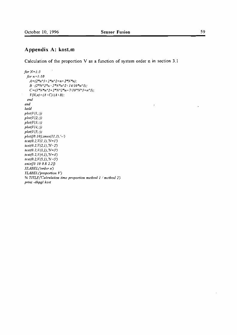
October 10, 1996

Appendix A: kost.m

Sensor Fusion 59

Calculation of the proportion V as a function of system order n in section 3.1

for N=1:5for n=1:10

A =(2*nI\3+ 2*nI\2+n+ 2*N*n);B=(2*NI\2*n+ 2*N*n1\2+ 1411O*nI\3);C=(3 *N*nI\2+ 2*NI\2*n+ 7110*NI\3+nI\3);V(N,n)=(A+C)I(A+B);

endendholdplot(V(1,:))plot(V(2,:))plot(V(3,:))plot(V(4,:))plot(V(5,:))plot([O:1OJ.ones(11.1), '--?text(0.2, V(1,1), 'N=1?text(0.2, V(2,J), 'N=2?text(0.2, V(3, 1). 'N=3?text(0.2, V(4,1), 'N=4?text(0.2, V(5.1). 'N=5?axis([O 100.8 2.2j)XLABEL('order n?YLABEL('proportion V?% TITLE('Calculation time proportion method 1 1 me'thod 2?print -dhpgl kost

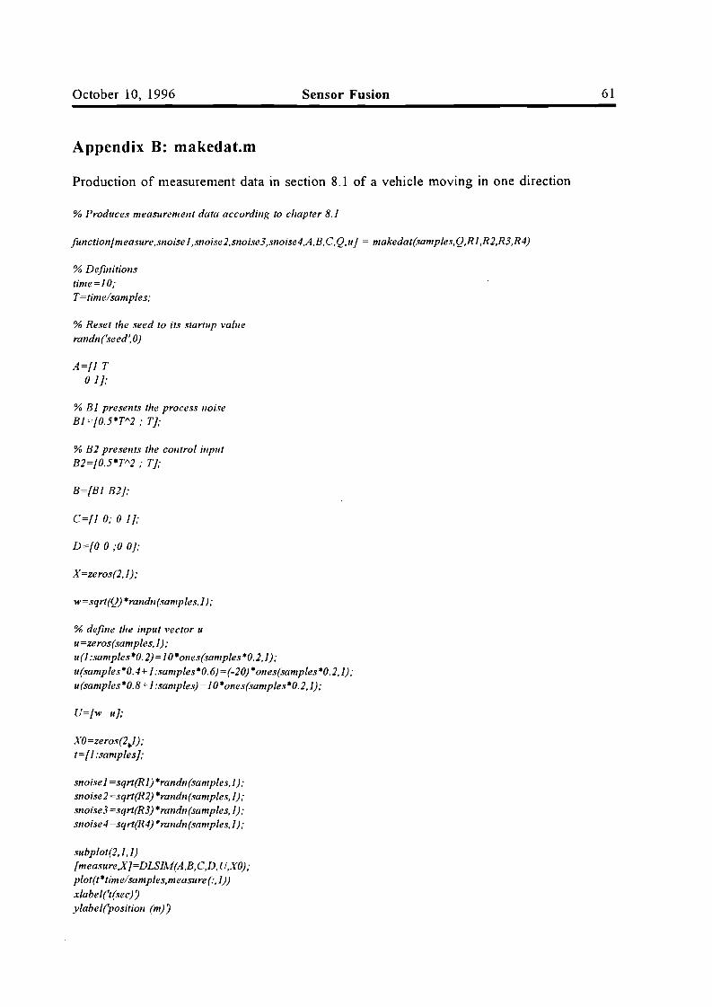
October 10, 1996

Appendix B: makedat.m

Sensor Fusion 61

Production of measurement data in section 8.1 of a vehicle moving in one direction

% Produces measurement data according to chapter 8.i

function[measure,snoise i ,snoise2,snoise3,snoise4.A.B. C,Q. uJ = makedat(samples.Q.Ri ,R2,R3.R4)

% Definitionstime=iO;T=time/samples;

% Reset the seed to its startup valuerandn(seed'.O)

A=[i To i];

% Bi presents the process noiseBi=[0.5*F'2; T];

% B2 presel/ts the cOl/trol iI/putB2=[0.5*TI\2 ; T];

B=[Bi B2J;

C=[i 0; 0 i];

D=[O 0 ;0 OJ;

X=zeros(2,J);

w =sqrt(Q) *randn(samples, i);

% define the input vector uu=zeros(samples.i);u(l :samples*0. 2) =i 0 *0Iles(wmples*0.2.i);u(samples*0.4+ i :samples*0. 6) = (-20) *ones(samples*0. 2, i);u(samples*0.8+ i :samples) = iO *0Iles(mmples*0.2. i);

U=[w u];

XO=zeros(2..i);t=[i :samples];

slloisei =sqrt(Ri) *randn(samples,J);snoise2=sqrt(R2) *ral/dn(samples, i);snoise3 =sqrt(R3) *randn(samples.i);snoise4=sqrt(R4) *ral/dn(samples,J);

subplot(2.i.i)[measure,X]=DLSIM(A,B.C.D.U,XO);plot(t*time/samples.measure(:. i))

xlabel('t(sec) Jylabel('position (m) J

62

subplot(2,l,2)plot(t*time/samples,measure (:,2))

xlabel('t(sec) ')ylabel('speed (m/s) ')V=axis; V(3)=-40; axis(V);

print -dhpgl g:\verslaglchap81



Appendix C: central.m and centr82.m

Matlab function containing the central fusion algorithm as described in this reportcentral.m:% Central fusion. chapter 3 for N sensors

function [Xglob,Pglob,Xpred.Ppredj=centraI(A.B.H. Q. u,R.2.Xin i t.Pinit)

RINV=inv(R);

% calculations according to equations 3.6 alld 3.7Xpred=A *Xinit+B(:.2) *u;Ppred=A *Pinit*A'+B(:.I) *Q *B(:, I) ';

% calculation according to equation 3.5Pglob=inv(inv(Ppred)+H'*RINV*H);

% calculation according to equation 3.4Xglob = Xpred+ Pglob *H '*RIN F* (Z-H *Xpred);

Matlab file using function central.m in the 2 position sensor case.centr82.m:samples=500;Q=O.I;RI=1;R2=1;R3=1;R4=1;[measure,n 1.n2,n3.n4.A.B.C,Q,uj = makedat(samples.Q.R1.R2.R3.R4);21 =measure(:,1)+n1;22=measure(:.1)+n2;

2=[21 22]';H=[l 0; 1 OJ;R=diag([R1 R2j);

Xinit=ze ros(size (A,1).1);Pinit=diag([Q Qj);P(1)=Q;X(1)=O;

for i=2:samples[Xglob.Pglob,Xpred.Ppredj = central(A.B.H.Q.u(i-1).R,2(:.i),Xinit,Pi1lit);Xi1lit=Xglob;Pi1lit=Pglob;X(i)=Xglob(1);P(I} =Pglob(1. 1);

end

1loise =X'-measure(:, 1);%mea1l(1loise (1 OO:samples))%var(1loise(100:samples))

subplot(2,1 ,1)


plot(!1:500j*0.02,noise)Title(['Ri = ',num2str(Rl), ' and R2= ',num2str(R2)J)xlabel('t(sec) Jylabel('noise (m) Jtext(1,O.I,['mean noise: ',num 2str(mean(noise(I OO:samples)))J)text(6,0.I,['var noise: ',num 2str(var(noise(1 OO:samples)))J)

subplot(2,I.2)plot(!1:500j*0.02,P)xlabel('t(sec) Jylabel('P(1,I))

%print -dhpgl g:\verslaglchap822


Appendix D: hier.m and hier82.m

Matlab function containing the hierarchical fusion algoritm as described in this reporthier.m% Hierarchical fusion, chapter 4 for N sensors

function[Xg10b.Pglob}=hier(A, B, Q.u.xinit,Pinit, P10c.Plocpred.xloc.xlocpred)

n=size (ploc, 2);N=size(ploc, I)/size(ploc, 2);

% calculations according to equations 3.6 and 3.7Xpred=A ·Xinit+B(:, 2) ·11;Ppred=A ·Pinit·A '+B(:,I) ·Q·B(:, I) ';

% calculation accordillg to equation 4.2Pglob =inv(ppred);for i=I:N

Pglob =Pglob+ (inv (Ploc((i-I) ·n+ 1:i·n, .j) - inv(plocpred((i-I) .//+ 1:i·n,.j));endPglob=inv(pglob);

% calculation according to equation 4.3Xglob =Xpred;for i=I:N

Xglob=Xglob+Pglob • (inv(ploc ((i-I) ·n+ 1:i·n,:)) • (Xloc((i-I) .//+ 1:i·n,.j-Xpred));Xglob=Xglob+Pglob ·(inv(plocpred((i-I) ·n+ 1:i·//,)) • (Xpred-Xlocpred((i-I) ·n+ 1:i·n.)));

end

Matlab file using function hier.m in the 2 position sensor case.hier82.msamples=500;Q=O.I;RI=I;R2=1;R3=1;R4=1;[measure.nl.n2,n3.n4.A.B,C,Q,II} = makedat(samples.Q,RI,R2,R3,R4);21 =measure(:,I)+nl;22=measure(:, 1)+ n2;

XI init=zeros(size(A, I), I);P linit=diag([Q Q});X2init=zeros(size(A.I).I);P2init=diag([Q Q});Xinit=zeros(size(A.I).I) ;Pinit=diag([Q Q});X(l)=O;

for i=2:samples%local filter 1[XI,Pl.x1pred,PIpred}=central(A,B.[1 0},Q,II(i-I),RI,21 (i).xl init,Plinit);XI init=XI;

66

P 1init=P1;

Senso." Fusion 10 October 1996

%10cal filter 2[X2,P2,X2pred,P2predJ=central(A,B.[1 0J,Q,u(i-1),R2,Z2(i)'x2init,P2init);X2init=X2;P2init=P2;

Xloc=[X1; X2J;Ploc=[P1; P2];Xlocpred=[X1pred; X2predJ;Plocpred=[P1pred; P2predJ;

%fusion of local filters with !tier.m[Xglob,PglobJ=h ier(A,B.Q. u(i-1) ,Xinit,Pinit,P10c,Plocpred,Xloc,Xlocpred);Xinit=Xglob;Pinit=Pglob;X(iJ =Xglob(1);

end

noise =X'-measure(:,1);%mean(lloise (1 00:samples))%var(lIoise(100:samples))

subplot(2,1,1)plot([1:500]*0.02,noise)Title(['R1=',num2str(R1),' and R2=',num2str(R2)J)xlabel('t(sec) ')ylabel('noise (m)')text(1,O.1,['meall noise: ',lIum2str(mean(noise(100:samples)))J)text(6,O.1,['var noise: ',lIum2str(var(noise (1 OO:samples)))J)

subplot(2,1,2)plot([1:500]*0.02,P)xlabel('t(rec) ')ylabel('P(1, 1) ')


Appendix E: hierfeed.m and hierfe82.m

Matlab function containing the hierarchical fusion algorithm with feedback as described in thisreporthierfeed.m% Hierarchical fusion with feedback, chapter 5 for N sensors

function[Xglob ,Pglob)=hierfeed(A,B, Q, u,Xinit,Pinit,P10c,P10cpred,X10c,Xlocpred)

n=size(Ploc, 2);N=size(Ploc,I)/size(Ploc,2);

% calculations according to equations 3.6 and 3.7Xpred=A *Xinit+B(:,2) *u;Ppred=A *Pinit*A '+B(:, I) *Q *B(-,I)';

% calculation according to equation 5.2Pglob =(1-N) *inv(Ppred);fori=I:N

Pglob =Pglob+ inv(Ploc((i-I) *1/+ 1:i*1I,:));endPglob =inv(Pglob);

% calculation according to equation 5.3Xglob=Xpred;for i=I:N

Xglob=Xglob+ Pglob *i1lv(Ploc((i-l) *11+ 1:i*I/,:)) *(Xloc((i-I) *1/+ 1:i*1I,:)-Xpred);e1ld

Matlab file using function hierfeed.m in the 2 position sensor case.hierfe82.msamples=500;Q=O.I;RI=I;R2=I;R3=I;R4=I;[measure,nI,n2,n3,n4,A,B,C,Q,u] = makedat(samples,Q,RI,R2,R3,R4);ZI =measure(:,I)+nI;Z2=measure(:, 1)+n2;

Xl in it=zeros(size(A, 1),1);P1init=diag([Q Q));X2init=zeros(size(A,I),I);P2init=diag([Q Q));Xinit=zeros(size (A, 1),1);Pinit=diag([Q Q));X(I) =0;

for i=2:samples%local filter 1[XI,P1,Xlpred,PIpred)=celltml(A,B.[1 O),Q,u(i-I),RI,ZI (i),):Iinit,P iiI/it);

68 Senso.' Fusion 10 October 1996

%Iocal filter 2[X2,P 2,X2pred,P2predI=central(.4,B,[J 0I,Q,u(i-J),R2,Z2(i)'x2init,P2init);

Xloc=[XJ; X2I;Ploc =[PJ; P2I;Xlocpred=[XJpred; X2predI;Plocpred=[P Jpred; P2predI;

%Jusion oj local filters with hier.m[Xglob,PglobI=hierJeed(A,B, Q, u(i-J) ,XiIIit,Pillit,Ploc,P10cpred,Xloc,Xlocpred);

Xinit=Xglob;Pinit=Pglob;

%Jeedback ojglobal state estimate and global covariance to the local%estimators, according to equatiolls 5.4 and 5.5X Jinit=Xglob;P Jinit=Pglob;X2init=Xglob;P2init=Pglob;

X(i)=Xglob(J);end

noise =X'-measure(:, J);%mean(noise(lOO:samples))%var(noise(J OO:samples))

subplot(2,J,l)plot([J:500]*0.02,noise)Title(['RJ = ',num 2str(RJ), ' and R2 =',num2str(R2)I)xlabeI('t(sec) ?ylabel('noise (m))text(l ,0. J ,['mean noise: ',num2str(mean(noise(l OO:samples)))I)text(6. O. J,['var noise: ',nllnt 2str(var(IIoise(l OO:samples))) I)

subplot(2,J,2)plot([J :500]*0.02,P)xlabel('t(sec) ?ylabel('P(l,J))


Appendix F: hierred.m and hierre82.m

Matlab function containing the hierarchical fusion algorithm with reduced feedback as described inthis report.hierred.m% hierarchical fusion with reduced feedback. chapter 5.3 for 2 sensors

function [Xglob.Pglob]=hierred(A.BH. Q, u,R2,Xini t.Pinit,Ploc,Plocpred,Xloc,Xlocpred)

n=size(ploc,2);N=2;

% calculation equation 5.1"Kfusion=Ploc(I :n,.~ *H (2.:) '*inv(H(2,) *Ploc(I :n.:) *H (2,.~ '+R2);

% calculation equation 5.13Pglob=(eye(n)-Kfusion *H(2.)) *Ploc(l :n.);

% calculation equation 5.12Xglob=Pglob *(inv(ploc(l:n,)) *Xloc(I :n,) +inv(ploc(n+ 1:2 *n,:)) *Xloc(n+ 1:2 *n,)-(inv(ploc(n+ 1:2 *n,:))-H(2.:) '*inv(R2) *H(2,)) *Xlocpred(n+ 1:2*n,:));

Matlab file using function hierred.m in the 2 position sensor case.hierre82.msamples=500;Q=O.I;RI=I;R2=I;R3=I;R4=I;[measure.nI.n2.n3.n4,A.B,C,Q.u] = makedat(samples.Q.RI.R2.R3,R4);ZI =measure(:,I) +nI;Z2=measure(:,J) +n2;

XI init=zeros(size (A. 1), 1);PI init=diag([Q Q]);X2init=zeros(size(A, 1).1);P2init=diag({Q Q]);Xinit=zeros(size(.4, 1). 1);Pinit=diag({Q Q]);X(1)=O;

for i=2:samples%local filter 1{XI.P1,XIpred,PIpred]=central(A,B.{1 0}.Q,u(i-I),RI.ZI (i),Xlinit,Plin it);

%local filter 2{X2,P2,X2pred.P2pred]=central(A.B.{1 0].Q. u(i-I).R2,Z2(i) ,X2init.P2init);X2init=X2;P2init=P2;

Xloc={XI; X2];

70

Ploc=[P1; P2];Xlocpred=[X1pred; X2pred];Plocpred=[P1pred; P2pred];


%fusion of local filters with hierred.m[Xglob,Pglob]=hierred(A,B.[ I 0 ;1 0],Q,u(i-1),R2,Xinit,Pinit,Ploc,Plocpred,Xloc,Xlocpred);

Xinit=Xglob;Pinit=Pglob;

%feedback ofglobal state estimate and global covariance to the local%estimators, according to equations 5.4 and 5.5X1init=Xglob;P linit=Pglob;

X(i) =Xglob(l);end

noise =X'-measure(:, 1);%mean(noise(lOO:samples))%var(noise(lOO:samples))

subplot(2,l,1)plot([l :500]*0.02,noise)Title (['R1 = ',num2str(Rl), , alld R2= ',lIIlm2str(R2J])xlabel(t(sec) )ylabel(noise (m))text(l,O.l,['mean noise: ',nllm 2str(mean(noise(l OO:samples)))J)text(6,0.l,['var noise: ',nllm 2str(var(noise(l OO:samples)))])

subplot(2, 1,2)plot([1:500]*0.02,P)xlabel(t(sec) )ylabel('P(l, l) ')

eindhoven university of technology master sensor … · eindhoven university of technology ... the...

Documents