Eindhoven University of Technology

MASTER

Optimizations for the implementation of a turbo decoder

Maessen, F.A.M.

Award date:2000

Link to publication

DisclaimerThis document contains a student thesis (bachelor's or master's), as authored by a student at Eindhoven University of Technology. Studenttheses are made available in the TU/e repository upon obtaining the required degree. The grade received is not published on the documentas presented in the repository. The required complexity or quality of research of student theses may vary by program, and the requiredminimum study period may vary in duration.

General rightsCopyright and moral rights for the publications made accessible in the public portal are retained by the authors and/or other copyright ownersand it is a condition of accessing publications that users recognise and abide by the legal requirements associated with these rights.

• Users may download and print one copy of any publication from the public portal for the purpose of private study or research. • You may not further distribute the material or use it for any profit-making activity or commercial gain

Optimizations forthe implementationof a turbo decoder

Francien Maessen

November 2000

Supervisors:

Dr. Ir. F.M.J. Willems (Eindhoven University of Technology)

Prof. Dr. Ir. G. Brussaard (Eindhoven University of Technology)

Prof. Dr. Ir. L. van der Perre (IMEC)

Abstract

Turbo decoding techniques achieve near-optimal performance in terms of BitError Rate (BER) at low Signal to Noise Ratios (SNR's). Amongst thesetechniques, convolutional turbo codes and product turbo codes are nowadays themost common ones. They have already been selected as a standard for theUniversal Mobile Telecommunication System (UMTS) [Lit. 4]. In the future, theywill probably also be selected as a standard for Wireless Local Area Networks(WLAN).

For such high-speed wireless applications, throughput and energy consumptionare crucial issues. By contrast, the hardware implementation of the turbo codes israther slow and power consuming. Therefore, the implementation of turbodecoders needs to be optimized.

Since an analysis of the energy consumption and throughput in turbo decodershas indicated a bottleneck in memory accesses, a systematic data transfer andstorage optimization methodology, developed at IMEC, has been applied. Itreduces the energy consumption and latency; in addition, it allows reachinghigher data rates. The whole methodology has been applied to the convolutionalturbo decoder, while for the product turbo decoder only some global optimizationshave been exploited.

Based on a high-level memory- and architectural model, estimations have beenmade for area, energy per bit, throughput and latency at a constant clockfrequency of 77 MHz. For the convolutional turbo code, a 25-fold energyreduction per decoded bit has been achieved, while at the same time the speed ismultiplied by 400 and the latency divided by 400. These results have beenachieved at the cost of the logic- and memory area: the total area consumption isincreased by a factor of 5. The results of the product turbo code show a gain inboth energy- and area consumption: the energy consumption per decoded bit isdecreased with a factor 5 and the area consumption is decreased with a factor 3.For the throughput and latency of the product turbo code, no estimations havebeen made in this report.

The energy consumption per decoded bit of the convolutional turbo code afteroptimization (0.04 I-lJ) has acceptable levels for an implementation at high data­rates. The product turbo code, however, still needs some optimizations before itcan be implemented on a single chip, as the energy consumption per bit (0.6 I-lJ)is still too large for a high-speed implementation.

2

Acknowledgements

I am indebted to many people for their advice, assistance and contributions to myproject on turbo coding.

First, I wish to thank the people at fMEC with whom I had many discussions andwho gave me much inspiration. I especially would like to thank my supervisor atIMEC, Liesbet van der Perre, for her support on this project. She introduced meto "the world of scientists" by making me co-writer of some papers ([Lit. 22] and[Lit. 25]) and letting me submit a paper [Lit. 26] at the Symposium of VehicularTechnology and Communications. Furthermore, she gave me the opportunity togo to the 2nd International Symposium on Turbo Codes in Brest, which was awonderful experience. My special thanks also to Marc Engels who gave me hissupport when Liesbet took maternity leave.

Furthermore, I would like to thank my supervisors from the Eindhoven Universityof Technology. First, I wish to thank Frans Willems, my direct supervisor, for hisconstant support and encouragement throughout the whole work on this project.He also advised me to work on the implementation of turbo decoders instead ofthe algorithm itself. Although I doubted his advice in the beginning, I am very gladthat I took the decision to work on the implementation: it has been a veryinteresting project. In addition, I would like to thank my other supervisor from theEindhoven University of Technology, Gert Brussaard, for his support. At times thatI needed him, he was always ready to help.

Last, but not least, I would like to thank my boyfriend Arjan Mels for the manydiscussions and inspirations, for reviewing my report and for his constant support.

Francien Maessen

3

Table of contents

Abstract 2

Acknowledgements 3

Table of contents 4

1 Introduction 6

2 Fundamentals of convolutional turbo coding 7

2.1 The general transmission scheme 7

2.2 Encoding 8

2.3 Channel 8

2.4 Decoding 9

2.5 Convolutional codes 10

3 Basic implementation of the MAP-algorithm 15

3.1 Basic implementation 15

3.2 Identifying the bottlenecks 15

4 Optimizations for the convolutional turbo decoder 21

4.1 Data Transfer and Storage Exploration methodology 21

4.2 Global loop transformations 22

4.3 Memory hierarchy 25

4.4 Memory allocation 30

4.5 Data-flow transformations 34

4.6 Optimized convolutional decoder 36

5 Product turbo code 38

5.1 The algorithm 38

5.2 Optimizations for the product turbo decoder 40

5.3 Results 42

6 Conclusions 44

7 Future work 45

Acronyms 47

Literature 48

4

Appendix A Alcatel 0.35-l..Im CMOS technology 50

A.1. Memories 50

A.2. Registers 50

A.3. Arithmetic units 50

A.4. Length of the critical path 51

Appendix B Mathematical derivations in the MAP-algorithm 52

B.1. Derivation of the LLR 52

B.2. Logarithmic notation for LLR 53

B.3. Logarithmic notation for metric 54

B.4. Logarithmic notation for extrinsic information 56

Appendix C Implementation of calculations 57

C.1. Basic implementation metric calculation 57

C.2. Basic implementation input calculation 58

C.3. Basic implementation subtractive normalization 59

C.4. Basic implementation extrinsic output... 60

C.5. Optimized implementation metric calculation and normalization 61

Appendix D Computations on the convolutional turbo code 62

0.1. Computations after loop transformations 62

0.2. Computations after introducing a memory hierarchy 63

0.3. Computations after memory allocation 63

0.4. Computations after data-flow transformations 64

Appendix E Output from ATOMIUM 66

Appendix F Derivation of LLR for product codes 67

Appendix G Sorting algorithms 68

G.1. Bubble sort 68

G.2. Shell's law 68

5

1 Introduction

Noise in a transmission channel is the limiting factor for the faithful replication of atransmitted signal. Shannon stated that it is possible, however, to establish error­free communication below a certain data-rate limit [Lit. 1]. This limit is called theShannon capacity limit. Finding codes that operate near the Shannon capacitylimit with a tolerable complexity is a challenge in information- and coding theory.

In [Lit. 2] a new class of codes, called turbo codes, was presented. Theperformance of these codes is close to the Shannon limit. A typical turbo codeconsists of two rather simple codes concatenated by an interleaver. For thesesimple codes, either convolutional- or product codes are commonly used. Themain innovation of turbo decoding is to perform the decoding iteratively wheresoft output information of the first decoder is passed on to the input of the seconddecoder. Then the soft output of the second decoder is fed back to the firstdecoder and so on. This functionality reminded the authors of [Lit. 2] of a turboengine and inspired them to this name.

The outstanding Bit Error Rate (BER) performance of this coding scheme createda large interest in turbo codes due to the wide range of possible applications. Forexample, a recent proposal for the Universal Mobile Telecommunication System(UMTS) for 3'd generation mobile communication includes a turbo-coding scheme[Lit. 4].

However, the implementation of a turbo decoder faces a number of challenges.LlMTS applications and Wireless Local Area Networks (WLAN) for exampledemand a high-throughput decoder. This report focuses on the implementation ofa turbo decoder that will be used for WLAN. Since this application needs a high­throughput decoder, the energy per decoded bit has also to be minimized in orderto get reasonable power consumption.

With the purpose of reaching a higher throughput and lower energy consumption,we have applied a systematic data transfer and storage optimization teChnique,developed at the Inter-university Micro-Electronic Center (IMEC) [Lit. 5], to theturbo decoder. The whole methodology has been applied to the convolutionalturbo code. The first global optimization steps have been investigated for theproduct turbo decoder in order to initiate a comparison with the convolutionalturbo decoder.

This report is organized as follows: in Chapter 2, the fundamentals of coding andespecially the turbo coding theory for convolutional turbo codes are explained;Chapter 3 describes the basic implementation of the convolutional turbo decoderand the bottlenecks of this implementation; Chapter 4 explains the optimizationsapplied to the convolutional turbo code; Chapter 5 describes the product turbocode and the optimizations applied to this code; finally, conclusions andrecommendations can be found in Chapter 6 and Chapter 7.

6

2 Fundamentals of convolutional turbo coding

The goal of communication is to send messages from one point to another.Before sending, the messages are translated into physical properties, forexample into electrical voltages. These electrical signals can be transmitted overa link, usually called the transmission channel. Unfortunately, the transmissionchannel adds noise to the transmitted signal. This noise leads to detection errorsat the receiver side. The aim of the communication system is to reduce thenumber of transmission errors as much as possible.

In [Lit. 1], Shannon introduced the concept of channel capacity. He showed that itis possible to transmit information over a channel with an error probabilityapproaching to zero for every rate less than the channel capacity. In [Lit. 2] a newclass of codes with a performance close to the Shannon limit was presented.These codes are called turbo codes.

This chapter first describes the general model of a transmission scheme;subsequently, some elements of this scheme are explained for convolutionalturbo codes in more detail.

2.1 The general transmission scheme

Figure 2.1 shows a block scheme of the transmission process. This processstarts with generating binary information at the transmitter side that is split into so­called frames. These frames are fed into the encoder. The encoder adds n-1

I transmitter ~C;__,,_,c,_.~--.l~1 encoderc, ...C,

~I modulator ~ X, ... x,

• Figure 2.1: general transmission schemel

redundant bits ((',1" •••<'''-' )to each input bit (c;' ) within a frame. The notation for

the produced sequence of symbols generated by the encoder is given below.

l(C;:,

c = C,r •

C/:'H

C/,'E{O,I}, fE[l,N], kE[I,n-l] (2.1 )

This sequence is the input to the modulator. The transformation of this sequenceto a signal, which can be sent over the channel, can be done in various ways.

1 This scheme is a simplified scheme and does not include for example compression

7

The transformation is for instance Binary Phase Shift Keying (BPSK). Thesequence is thus transformed by using the transformation: {0,1} ~ {-1,1} .

Hence, each symbol that is inserted into the channel can be calculated by

X, =2·C,-1 (2.2)

The channel distorts the signal so that the decoder on the receiver side receivesthe sequence YI ... YN instead of CI ... CN. The decoder provides an estimate CI

... CN of the sent sequence.

In the following sections, the encoder, the channel and the decoder will beexplained in more detail.

2.2 Encoding

The aim of an encoder is to map theincoming message to a code word.Figure 2.2 represents the encodingpart of a turbo code: a parallelconcatenation of two rather simpleconvolutional encoders (C1 and C2). 'i""NThe output symbol Ct of the turboencoder is a combination of theoriginal (systematic) sequence, onecheck bit from C1 and one check bitfrom C2 (the parity bits). The input toC1 is the original data sequence, while • Figure 2.2: turbo encoderan interleaver TT reorders the input toC2. Interleaving is done so that theinverse operation at the receiver side spreads neighboring errors. These spreaderroneous symbols are less correlated for the decoder.

2.3 Channel

As explained before, time discrete signals with values -1 and + 1 are sent over achannel. If + 1 has been transmitted whereas the decoder estimates -1 due to thenoise in the channel, a bit error occurs. The noise in a channel highly depends onthe type of the channel. This section briefly describes the Additive WhiteGaussian Noise (AWGN) channel and the Rayleigh fading channel.

2.3.1 AWGN channel

The noise n of the AWGN channel ismodeled by a zero-mean normallydistributed random signal of varianceif = Nr/2. No denotes the one-sidedspectral noise density. Let Es be theaverage energy received for eachsymbol. Then Es INa is defined as theSignal to Noise Ratio (SNR).

8

yt

• Figure 2.3: Gaussian model

The noise is additive. The received signal is thus: Yt =Xt + nt.. The AWGN channelis described by the following Power Distribution function (PDF) of the receivedsignal:

(2.3)

The PDF model for the Gaussian channel is illustrated in Figure 2.3.

2.3.2 Rayleigh fading channel

Channels that change their properties (for example due to mUlti-path propagationin mobile communications) during the transmission are called time varying. Anexact model of these channels is very complex. That is why the model issimplified to the main properties of the channel, namely the value and thecorrelation of the received signal amplitude. A Rayleigh fading channel is in thestudy of communication systems an AWGN channel with varying signal amplitudeat:

Y, =a, . x, + 11,

p,(a)

The mUltiplicative deterioration at isRayleigh distributed [Lit. 6] and given bythe following formula:

The model for the Rayleigh distribution isrepresented in Figure 2.4.

The Rayleigh channel is thereforedescribed by the following PDF for thereceived signal:

p(vlax)= 1 .expl(-(yl-a,xIYJ., I I .J21la 2 2a 2

2.4 Decoding

• Figure 2.4: Rayleigh distribution

a

(2.4)

Turbo decoding is based on an iterative process, where two soft output decodersuse each other's (interleaved) output as a-priori information.

The turbo decoding principle is outlined in Figure 2.5. Each encoder Ci of Figure2.2 corresponds to a soft output decoder Di in Figure 2.5. The decoder operateson three input sequences: the original input and the convoluted sequence of theappropriate encoder, which have been transmitted over a channel and the a-prioriinformation that is given by the previous decoding step. In the first decoding step,the a-priori information is 0.5 both zero and one. The decoding starts with 01.The output of this decoder lies in the range [-1,1]. The sign of the output gives thehard decision, while the absolute value gives information concerning the reliabilityof the hard decision. The output is split into channel values, a-priori information

9

) .5 ).5I"'N r---. output

TT

and extrinsic information. Thesecond decoder 02 uses theinterleaved extrinsic informationfrom 01 as a-priori information. Theflow of the extrinsic information issymbolized with gray arrows inFigure 2.5. In the next iteration (acombination of 01 followed by 02 iscalled an iteration), 01 is executedagain, now using the de-interleavedextrinsic information from 02 as a­priori information. This loop iscontinued until some stop criterion ismet.

• Figure 2.5: turbo decoder There is no fixed rule when to stopthe iteration process although some

criteria have been recommended in [Lit. 7] and [Lit. 8]. A higher number ofiterations yields a better decoding performance but requires also a larger amountof time. Furthermore, the decoding gain of additional iterations decreases rapidly.

In the following section, the operation blocks of the encoder (C1, C2) anddecoder (01, 02) will be explained in more detail.

2.5 Convolutional codes

In the convolutional turbo coder, the convolutional code blocks are the mostimportant modules. Therefore, the principle of the convolutional- encoding anddecoding is given in this section.

2.5.1 Convolutional encoder

1----·'"

JI

A convolutional encoder performs a discrete convolution using binary additionand multiplication: the input bits are sent through a shift register of known lengthm, while the output is a linearcombination of the differentregister contents that areformed by using theparameters aD, ai, ... am(Figure 2.6). The 0 operatordescribes a delay of oneregister cell. When the codeis recursive, another linearcombination of the registercontents is fed back to theinput of the encoder. Thisfeedback is described by the • Figure 2.6: systematic convolutional encoder

parameters b j , b2, ... bm.

Since all operations within the convolutional encoder are linear, the convolutionitself is also linear. The resulting convolution can be described by the followingtransfer function:

D D ill

C(D) = an +°1 + +° 111

I +bI D+ +b,,,D III

(2.5)

10

The code is called a systematic code if the input bit is also fed to the outputwithout coding (like in Figure 2.6).

A sequence of transitions in a Finite 8tate Machine (F8M) can describe theencoding process: the register content is represented by the current state Si,

denoted as St. Given the current state, the next input bit determines the nextstate. The output bit for a certain state-transition depends on three items: thecurrent state, the input bit and the implementation of equation 2.5. The statetransitions can be illustrated by a trellis graph showing the transitions betweenthe different states.

5, 5, 5, 5, 5, 5 s

• Figure 2.7: trellis of a four-state convolutional code

Figure 2.7 shows an example of the coding process by using a trellis. 80lid linescorrespond to transitions caused by the input of a 0; dashed lines denote theinjection of a 1. Given a transfer function with a nominator 1 + d and adenominator 1 + 0 + d, input {0,1 ,0,0,1} produces an output {0,1, 1,0,1} of theencoder. The resulting path {80 , 8 1, 8 2, 8 3 , 84, 8 5} = {so, so, S2, S3, S1, so} ishighlighted in Figure 2.7. If the code is systematic, the following symbols will betransferred to the modulator:

By convention, the encoder starts in a known state: the all-zero state (80 = so). Incertain cases, the encoder must end in a known state too. This can be achievedby forcing the encoder to a certain state by injecting m tail bits. The value of thetail bits depends on the current state of the F8M.

In this project, we assume a 8-state convolutional code with the following transferfunction:

(2.6)

2.5.2 Convolutional decoder

The decoder module is the most complex block in the convolutional turbodecoder. The module can be implemented in several ways. In this report, theMaximum A-Posteriori (MAP) decoding algorithm introduced by Bahl et. al. [Lit. 9]

11

is used for decoding. The MAP-algorithm did not become very popular untilrecently because of its large latency and high energy consumption compared tofor example the Viterbi algorithm [Lit. 3], which has a similar performance for lowBER's. However, turbo codes have changed the popularity of the MAP-algorithmbecause they require soft output and the algorithms like the standard Viterbialgorithm do not provide this.

The MAP-algorithm has three inputs: a systematic input, an encoded input and a­priori information (see Figure 2.5). These inputs are used for calculating aforward- and a backward recursion. These calculations are done byreconstructing the trellis of the encoding process. An element within a recursion,called a metric, consists of a certain number of states that is defined by the trellisof the encoding process. A metric indicates the probability of occurrence for eachstate in the trellis. In order to calculate one output-bit (Cts), one metric from theforward recursion and one metric from the backward recursion is needed.

The metrics in the forward- and backward recursion are introduced as a,respectively f3 in [Lit. 9]:

at (S, ) =I a t- J (S'_I ). P'"etric-,ra"Si,io,.(St-I' S,)S,_I

/3r (S,) =I /3r+1 (S'+I)' P'''l'IriC-rmll'''irirlll(S" S'+I)5'+1

(2.7)

(2.8)

In order to compute these recursive values, a start value is needed. As saidbefore, state 0 will be the first state and the last state. Since the metrics indicatethe probability of the states, the initial value of the first state will be one, theothers zero. Using the forward- and backward probabilities, the bit probabilitiescan be determined:

P"-I'O'I"/iori(C;' =0) = )" a'_1 (s,)· P',/{.,riC-'f'{/lI.'i'iO,.(S', s)· /3, (s)(.\~B(J

P't-J'O'N/i/lri (c;' = 1)= ..>a r_1(s,)· P'lll'lric-trallsirioll (s' ,s)· /3r (s)(.'~BI

where Bj is the set of transitions S'-1 =S' -> S, =s such that c;' = i.

(2.9)

(2.10)

In the probabilities given above, the metric-transition probability (that is theprobability that a code word follows any path via state s at time t) is used. Thisprobability can be formulated as follows:

P'/I('rric-rmt1.l'iriOIl(S',s)=p(Sr =s,YrISr_1=s')

=p(Y IS =s' S = s). p(s =sis = s' C" =i)' p((>' =i)I /-1 'f ([-I' t t

where

• p(y, \Sr_1 = s', Sr = s) must be deduced from the channel characteristics

• p(Sr = .'lISt-! = s', c;' =i) is either 0 or 1 depending on whether the input of c;'

leads from state S'-1 =s' to Sf =S

• p(cr' =i) is the a-priori probability of the transition s' -> s

12

If the second probability is 1, the metric-transition probability can be written as:

Pm"lrIL-JrunH/I<Jn = p(r; leI)' p(c;' (s', s) =i) (2.11 )

With the Rayleigh model for the channel described in Section 2.3.2 andsUbstituting X as in equation 2.2, this results in:

_[ly,-a(2C/(;',,)-llI' JP 20- p( S (, ) .)

melrlC.:-lran.\'IllOn =e . c, S, S = 1 (2.12)

In order to generate one soft output decision, it is beneficial to formulate the bitprobabilities as a Log-Likelihood Ratio (LLR) for two reasons: the received valuescan be easily converted to a LLR and mathematical simplifications are possiblefor the MAP decoding algorithm when using LLR. The mathematical derivation forthe LLR is given in Appendix S. The outcome of this derivation is given below:

P (, -1)LLR (c;') = log (/-1''''/<''''1"1 \c:. -

~'-I)(H',erl(m (c, == 0)

2a ~ ) ~ )- .1 L .\ L .1- -2 . y, + u-{mort C, + e.xlrmS1C C,

a(2.13)

The first term in 2.13 is the systematic channel value and the second termrepresents the a-priori information that was inserted into the algorithm. The thirdterm is the extrinsic information. This extrinsic information is used as a-prioriinformation for the next decoding step (see Figure 2.5).

The derivation of the soft output shows a lot of multiplication and logarithmicfunctions. Due to this, a hardware implementation will be very expensive.Therefore, a transfer of the algorithm to the logarithmic domain is used. Thus,multiplication becomes addition.

A problem arises in the transformation of additions to the log-domain. Thisoperation will be depicted as @. Let CPI and CPz be two variables in the logdomain 1. An addition transformed to the log domain will look like:

q?1@ q?2 = Ink" + e iP,)

= max(q?j, q?2) + In(l + e-liP'-iP,l)

= max(q?j' q?2) + fc ~q?j - q?21)

= max" (q?j , q?2) (2.14)

This means that an operation @ can boil down to the maximum operation with acorrection function fe (max). The max· function is described in [Lit. 12]. However,using fixed point values, the compleXity of the implementation of the max*function can be significantly reduced. This implementation will be explained in thenext chapter.

In Appendix S, the logarithmic derivations for the LLR, the metric values and theextrinsic information are given.

1 the - indicates a variable in the log-domain

13

As mentioned before, the MAP-algorithm is the most important module within theturbo decoder. At the same time, it is also the most complex block to implement inhardware. In the next chapter, we will look at the basic implementation of MAP­algorithm in hardware.

14

3 Basic implementation of the MAP-algorithm

This chapter shows the basic implementation of the main building block of theconvolutional turbo decoder: the MAP-decoder. Given the basic implementation,we can identify the bottlenecks of the decoder in terms of energy, area,throughput and latency for applications like WLAN.

3.1 Basic implementation

T

,,~ k=frame size-' ~,

u /-' ~L"',,",,,

/,f-' ~k=O

K

As can be concluded from the algorithm description, the decoder producesextrinsic information using forward- and backward probabilities. Theseprobabilities are based on the entire frame: for the production of extrinsicinformation concerning the t-th bit, at-l and f3t have to be known. The moststraightforward implementation calculates the a's over the entire frame and then

the f3's and extrinsic information inthe backward direction, as shown inFigure 3.1. The x-axis indicates thetime, whereas the y-axis indicates therecursion- or output calculation of acertain bit. K is the frame-size and Tis the decoding latency for one half­iteration. The frame-size is assumed

• Figure 3.1: basic implementation of the MAP-decoder 400 in this report.

3.2 Identifying the bottlenecks

In order to identify the bottlenecks in the basic implementation of the MAP­algorithm, we have to make estimations for energy- and area consumption, aswell as for throughput and latency. All estimations for the basic implementationhave been based on the 0.35-lJm CMOS process of Alcatel Microelectronics.

3.2.1 Estimations for energy and area

The costs in terms of energy and area depend on three aspects: control, data­path calculations and memory.

The control can be implemented as a finite state machine (FSM). This FSM canbe easily implemented by using counters. Since the costs in terms of energy andarea for a counter are rather low (see Appendix A), we did not take into accountthe energy- and area consumption for the control.

In order to be able to estimate the energy- and area consumption in the data-pathand the memory, it should be identified:

• how the metric- and extrinsic calculations can be implemented in hardware;

• what the number of arithmetic operations, the number of memories and thenumber of accesses to these memories are;

• what the costs of a single arithmetic operation and a single memory (access) interms of energy and area are;

These three issues are investigated in the following sections.

15

Implementation issues for the calculations

For the implementation of the calculations in the MAP-algorithm, two issuesshould be investigated in more detail. First, a correction function is needed forcalculations in the log-domain, as explained in Section 2.5.2. Second, the a- andf3 values, calculated by recursion, can become very large: a normalizationscheme is needed here.

Logarithmic correction function

As explained before, the log-MAP-decoderhas a maximum function (max") that consistsof a maximum operation and a correctionfunction (equation 2.14). The implementationof the correction function is not complexbecause fixed-point values are used. Figure3.2 shows the correction function for floating­and for fixed-point values.

f(ct 0.8 '',0.7 !0.6 ;

0.5 L --·_··10.4

0.3

02

0.1

0.5

- Floating point

-----. Fixed point

1.5 2.5 3 3.5-c

if ( a < b) max' = a - f(c);else max' =b - f(c);

• Figure 3.2: the logarithmic correctionfunction

The implementation of the fixed-pointmax" function can be described asfollows:

c = (-c);f(c) = 0;f(c) = 0.25;f(c) = 0.5;f(c) = 0.75;

if (c < 0)if (c > 2)else if (c> 0.75)else if (c> 0)else

c = b - a;

IIl1UX* fUllction

• Figure 3.3: architecture for implementing the max'function Figure 3.3 illustrates the architecture

used for implementing the max"function. We have assumed 7 bits for the implementation of e, from which two bitsare used after the decimal point. f(e) consists of two bits: fde) and fo(c). Thesebits are described as:

fl(c) = chc, ,c4 ·(i\ -(2)

III (c) = ch . C, .c; .(c, .C2 + c2 . c1 . CIJ)

(3.1 )

(3.2)

Normalization

The second calculation issue that needs to be investigated is the normalization.The normalization of the metric calculation, needed to limit the number of bits in ametric word, relies on two properties: the output of the MAP-algorithm onlydepends on differences between metrics; and the difference between metrics isbounded. The two most common techniques for normalizing the metriccalculation are:

• subtracting the largest state of a metric from the other states of the metric

• using two's complement arithmetic

16

Before investigating these methods, it should be noticed that, due to the recursivedependency within the decoding algorithm, calculations in one trellis step have tobe conducted before the next step can be done. Additional calculations for thenormalization consequently increase the latency within the decoder.

The first technique, subtracting the largest metric from the others, is ratherstraightforward but adds some operations to the recursive path: comparisons toestimate the largest state of a metric plus a subtraction for every state.

The normalization technique using two's complement arithmetic [Lit. 10] does notavoid overflow, but accommodates overflow in such a way that it does not affectthe correctness of the results. In a common realization of two's complementarithmetic with n bits, both addition and subtraction are defined modulo ::t. Due tothis modulo operation, all values will lie on a circle. Figure 3.4 shows this circlefor a 3-bit word.

-1 Ol(}

III ()(1I

If the maximum difference between two values in two'scomplement arithmetic is less than half a circle, it isalways possible to determine which value is thelargest one. For example:

• Figure 3.4: example of metricrepresentation

110

0'III

J(I)

010

Oil

(+3)-(+1)=011 +111 =01 O=positive --> (+3) is the largestvalue(-1)-(-4)=111+100=011=positive --> (-1) is the largestvalue(-4)-(+2)=100+110=010=positive --> (-4) is the largestvalue

Note that because the maximum difference is less than four (half a circle), -4 islarger than 2.

This technique needs no calculations for normalization, so the decoding latency isnot increased by the normalization. However, additional calculations are neededfor the sign extension required in the soft output calculation (direct addition ofmetrics will exceed the maximum difference of half the cycle, loosing the propertyof knowing which one is the largest). Another disadvantage of this technique is,as simulations have shown, that three extra bits are needed for each metric word.One bit is needed for the sign extension. The need of the two other bits can beexplained by the fact that they are necessary to cover the whole range of valuesthat the metrics can have in the loss-less representation. This is not needed whensubtractive normalization is applied because the metric values are saturated then:the maximum state is then subtracted from the outcome of the metric calculation.

For the basic implementation, we assumed that the normalization was done byusing subtractive normalization. The implementation of the subtractivenormalization is given in Appendix C.

Appendix C gives also the basic implementation of the metric-, extrinsic- andchannel calculations, which we can derive from the MAP-algorithm.

Number of operations, memories and memory accesses

From the MAP-algorithm we can derive the number of metric-, extrinsic- andchannel calculations that we need. This gives the following results:

17

• Metric calculations: 2· frame _ size, 2 'number _ of _ iterations

• Subtractive normalization: 2, frame _ size, 2· number _ of _ iterations

• Extrinsic calculations: frame _ size' 2 ' number _ of _ iterations

• Channel calculations: 2, number_ of _ states· frame_ size' 2, number_ oj _ iterations

One metric calculation includes the calculation of all states in that metric. Theimplementation of the calculations is given in Appendix C. Every singlecalculation consists of the following operations:

• Metric calculation: 12 additions, 8 max* operations

• Subtractive normalization: 7 comparisons, 8 subtractions

• Extrinsic calculation: 20 additions, 14 max* operations, 1 subtraction

• Channel calculation: 1 or 2 additions

For estimating the number of memories, each array is supposed to be a memory.Within the MAP-algorithm, we have 5 arrays: 2 metric arrays in which we storethe recursive values and three input arrays: the systematic input array, the parityinput array and the a-priori array. We have deducted the number of maccesses tothese arrays from the MAP-algorithm itself:

• Metric array (for metric- and extrinsic calculation and subtractive normalization):(2,6, /lumber _ of _ states + 16 rjiwlle_ size' 2· number_of _ iterations

• Syst-input array (for metric calculation):(2, number _ of _ states), Fwne_ size' 2, /lumber _of _ iterations

• Parity-input array (for metric- and extrinsic calculation):(2, number _ of _ states + 4 rframe_ size' 2· nl.ll11ber_ of _ iterations

• A-priori array (for metric- and extrinsic calculation):(2, 1I1/lllber_ of _ states + I), ji'ame_ size' 2· nllmber_ of _ iterations

The number of states is eight (see also Section 2.5.1). The frame-size we havechosen is 400 and the assumed number of iterations is six. As can be concludedfrom the derivations above, the number of iterations will have no impact on therelative energy- and area consumption for the basic implementation.

Estimating costs in terms of area and energy for memories and calculations

We have estimated the energy- and area consumption using the 0.35-l-lm CMOSprocess of Alcatel Microelectronics. For the estimations, the word-lengths ofalphas, betas, channel- and extrinsic information have to be known. Aftersimulations with a fixed point C-code, we observed no significant performancedegradation for 7 bits for alphas and betas, 6 bits for the extrinsic information and4 bits for the channel information.

The costs of the memories in terms of area and energy are given respectively bythe formulas A.2 and A.1 in Appendix A. These formulas do not include the wireloads of the memories. We approximated the energy consumption due to theseloads as can be seen in Appendix A.

We have approximated the costs of the arithmetic operations in terms of energyand area by using a tool called SYNOPSIS (this tool simulates the hardwarelayout for a given VHDL code). The costs in terms of area are directly given by

18

SYNOPSIS. However, the costs in terms of energy cannot directly be givenbecause the switching activity of a single computation block is not known. To getan estimation of the energy consumption, an activity of 30% is typically assumed.The energy- and area consumption of the computation blocks is given inAppendix A.

Having investigated the three items that are necessary in order to estimate theenergy- and area consumption, we can approximate the energy- and areaconsumption within the MAP-decoder. Figure 3.5 lists some indicative figures.

Energy per bit(1.07 IJJ)

2%

88%

Area(3.53 mm2

)

65%

D Metric storaae

D Metric- and output calculation

• Input-/output storaqe

• Figure 3.5: relative area and energy consumption in the convolutional turbo decoder

3.2.2 Estimations for throughput and latency

In order to identify the bottlenecks in the implementation of the MAP-algorithm,we not only need estimations for the energy- and area consumption, but alsoestimations for the throughput and latency. The estimations for the throughputand latency will be investigated in this section.

The throughput and latency of the decoder depend on three factors: the delaycaused by the interleaver operation, the number of iterations of the MAP­algorithm within the decoder and the inherent decoding latency in MAP-algorithmitself. The latency of the interleaving operation is assumed to be zero (see alsoChapter 7). The number of iterations is assumed six. This iteration-number canbe limited by using an early stop criterion [Lit. 17]. However, we did not regard astop criterion in this thesis. The delay caused by the MAP-algorithm itself isinvestigated below.

The metric calculation forms the critical path within the MAP-algorithm. For theAlcatel 0.35-jJm technology, the length of the clock-cycle turned out to be 13 nsafter simulations with SYNOPSIS, which implies a clock-frequency of about 77MHz (see Appendix A). Given the clock-frequency, the throughput and latencycan be estimated when the number of clock-cycles that are needed to decodeone frame is known. All accesses to the metric memories that are needed for thecalculation of one single alpha or beta require one clock-cycle. Since the alpha­and beta calculations are recursive, all metric values within one frame have to becalculated serially. The total number of clock-cycles needed to decode one frameis 38400 (see also Appendix C):

• 48 clock-cycles are needed to calculate one metric consisting of eight states (fourmemory-reads and two memory-writes to the metric-memory for eight states ofthe metric).

• One half iteration contains 800 metric calculations (400 for the forward recursionand 400 for the backward recursion).

19

Given the clock-frequency and the number of clock-cycles within one frame, wehave estimated a maximum throughput of 804 kbitls and a minimum latency of5.9 ms when applying twelve half iterations in pipeline. When no pipelining isapplied, the throughput decreases to 67 kbitls, while the latency stays the same.

3.2.3 Overview of bottlenecks in the MAP.<fecoder

From the estimations for throughput and latency and from Figure 3.5 it can beconcluded that the area consumption is not a bottleneck for the implementation ofthe MAP-algorithm. However, the throughput and latency are respectively too lowand too high for applications like WLAN (36 Mbitls and 16 \.lS are neededrespectively). Moreover, the energy consumption per bit is a bottleneck if higherbit-rates are achieved.

The estimations for throughput, latency and energy consumption show that thebottlenecks are mainly caused by the data-flow dominated recursions in the MAP­algorithm. This implies that much can be gained if the data- transfer and storageis optimized. Therefore, we applied a data transfer and storage explorationmethodology developed at IMEC. The optimizations that we have applied byusing this methodology are described in the next chapter.

20

4 Optimizations for the convolutional turbo decoder

The analysis of the basic implementation of the MAP-decoder has indicated abottleneck in memory accesses. Thus, the memory architecture deseNes acareful analysis in the design process. Although considerable effort has alreadybeen spent on the implementation of the turbo decoder ([Lit. 10] and [Lit. 11]),memory organization has not been explored in depth up to now. For that reason,we have applied a systematic Data Transfer and Storage Exploration (DTSE)methodology, developed at the Inter-university Micro-Electronic Center (IMEC)[Lit. 5], to the MAP-algorithm. The goal of this methodology is to optimize theexecution order of the data transfers, in combination with the memoryarchitecture. This reduces the energy consumption and the latency of thedecoder. Furthermore, a higher throughput can be achieved.

Whether an optimization possibility exploited by the DTSE-methodology isbeneficial for implementation (in terms of energy, area, throughput or latency)most often depends on the process technology that is used. In this report, the0.35-l..lm CMOS process of Alcatel Microelectronics is assumed. Allapproximations for energy, area and timing have been estimated in the same wayas for the basic implementation in Chapter 3.

If an optimization possibility turns out to be constructive, a trade-off still has to bemade between energy, area and timing. Since the latency and throughput of thedecoder are the main obstacles to applications like WLAI\J, we considered timingas the most significant factor. A high-throughput also means that the energy perdecoded bit has to be minimized in order to get reasonable power consumption.

This chapter describes the application of the DTSE-methodology to the key­building block of convolutional turbo codes: the MAP-decoder; but first a briefintroduction to the DTSE-technique is given.

4.1 Data Transfer and Storage Exploration methodology

The DTSE-methodology allows to systematically reduce the storage bottleneck indata dominated algorithms such as the MAP-algorithm. The methodologyconsists of several steps:

1. Global loop transformations are carried out to reduce size of the system-levelbuffers caused by long delays between the production and the consumption of asignal;

2. A memory hierarchy is defined in order to benefit from the available temporallocality in the data accesses: frequently accessed data can be read from smaller,less energy consuming, memories;

3. Memory units are allocated and arrays are assigned to these memories, takinginto account the conflicts between arrays;

4. Data-flow transformations, such as modifying the computation order, shiftingdelay-lines through the algorithm or recalculation, are used to optimize energy­and area cost directly. Data-flow bottlenecks are removed as far as possible;

The DTSE-methodology normally applies data-flow transformations in the firststep. However, in the data-flow transformations for the MAP-algorithmcalculations will be traded off against memory accesses. In order to make

21

appropriate decisions for these transformations, the memory architecture has tobe known. For this reason, we investigate data-flow transformations in the laststep here.

4.2 Global loop transfonnations

As explained before, the throughput and latency are the main issues for theimplementation of the turbo decoder. In order to optimize the throughput andlatency, we have applied global loop transformations to the MAP-algorithm. Thegoal of these loop transformations is to parallelize the decoding process. Thissection describes the general method for parallelizing the MAP-algorithm.

4.2.1 General strategy

In order to parallelize the decoding process, a subdivision of the MAP-algorithminto smaller independent pieces is needed. The main problem in parallelizing theMAP-algorithm is the recursion of the state metrics a and /3: aN-1 recursivelydepends on all at, tE[O,N-2]; /31 depends on all /3t. tE[2,N). A modification of theMAP-algorithm is necessary to remove these dependencies.

4.2.2 Dummy metrics

The main idea of breaking the recursion sequence into several independentpieces is the assumption that the metrics are a function of only the previous Lrecursion steps. Any metric more than L steps before the current metric in therecursion has negligible influence on the decoding performance. Based on thisidea, [Lit. 13] and [Lit. 16] introduced sub-blocks of the MAP-algorithm, which arecalled windows. The MAP-algorithm containing windows has been namedOverlapping Sliding Window (08W) algorithm since these windows overlap eachother.

•••• dummy calculation

s

'..·.,~ull1my

•••• - • metric calculation

;'"_ metric- and extnnsic calculatIon

a; I;

..../L .--dummy...

I.

A window enabling parallelizationis pointed out in Figure 4.1. Thehorizontal direction indicates thetime, whereas the verticaldirection indicates the recursion­or output calculation of a certainbit. The goal of the scheme is tocalculate output without startingthe recursions at the beginningor at the end of the trellis: there • Figure 4.1: window for enabling parallelizationare no known a- or /3 statemetrics in this sub-block. The so-called dummies are initialized with uniform values because all states are equallylikely to have been visited during the coding process. After the initialization of thedummies, L recursion steps are carried out in order to obtain approximatelycorrect values for the initial a and {3. Given these values, reliable values for a and{3 can be calculated, each during S steps.

22

4.2.3 Overlapping windows

Using the approach with dummy metrics, an arbitrary number of windows can beprocessed in parallel. Figure 4.2 compares the parallelized MAP-algorithm withthe standard version.

2NT

~~..... ~~.....~..., ~

"..,.~ ..~....... ~

~

~.14

L I s [ S J(L+lS)T

....... dJmy caoJabrn

- - rrelnccaoJairn

- rreln<> ad extnme caoJairn

• Figure 4.2: comparison between standard an parallelized MAP-algorithm

The decoding latency 0 =2NT of the standard algorithm depends on the frame­length N. The latency in the parallelized version, however, depends on the lengthof the sequence of valid metrics calculated (25) and length of the sequence ofdummy metrics (L). The latency of the parallelized version consequently is (L +25)T. 5 can be varied to optimize the timing constraints. Simulations have shownthat for a dummy sequence length L 2: 18 the degradation in performance isnegligible.

4.2.4 Workers

The parallelization introduced in theprevious section uses windows that firstcalculate the a metrics, then the f3 metrics.Since the computation of a and f3 metrics isanalogous, it is also possible to construct awindow that first calculates the f3 metrics,then the a metrics. Both possibilities can befound in Figure 4.3. These windows are thesmallest sub-blocks that can exist in theparallel decoding of a complete block.

..........",/....

.......

• Figure 4.3: : two basic windows

'.'.. ~."".... ,").,,,

.....-"

The two basic windows can be combined in more than one way. Severalcombinations of windows are introduced in [Lit. 14] as workers. Some examples

of these workers are shown in Figure4.4. Some workers have time-slots inwhich valid a- and {3-values arecalculated simultaneously. Therefore,these metric values are being stored indifferent memories.

ba Every worker relies on an interactionbetween several windows. Because ofthis, not every dummy sequence has tobe calculated (see gray dots in Figure4.4). Furthermore, some workers make

memory reuse possible. This applies for worker a in Figure 4.4: when the firstwindow is producing output, it consumes a metrics that are no longer needed.

• Figure 4.4: different workers

23

The second window can then use this memory space. There is, however, also adisadvantage to the application of worker a: the decoding latency will increasebecause the second window starts later. Therefore, a trade-off has to be madehere between energy consumption, throughput and latency.

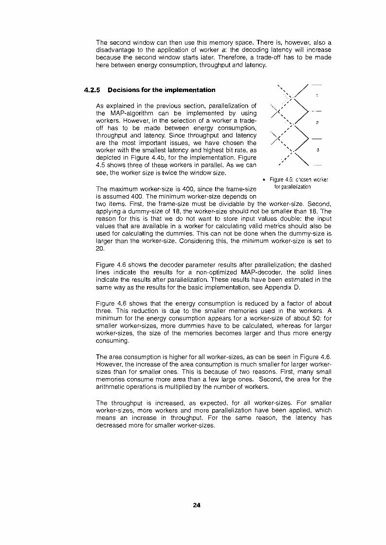
4.2.5 Decisions for the implementation

As explained in the previous section, parallelization ofthe MAP-algorithm can be implemented by usingworkers. However, in the selection of a worker a trade­off has to be made between energy consumption,throughput and latency. Since throughput and latencyare the most important issues, we have chosen theworker with the smallest latency and highest bit rate, asdepicted in Figure 4.4b, for the implementation. Figure4.5 shows three of these workers in parallel. As we cansee, the worker size is twice the window size.

"'. /-'» 1,'. ,.....:.<'...... -...... "

'» 2," ,..... .,,"

.:., -..... "

. ',. 3

.",' "'-, "'--

• Figure 4,5: chosen workerThe maximum worker-size is 400, since the frame-size for parallelizalionis assumed 400. The minimum worker-size depends ontwo items. First, the frame-size must be dividable by the worker-size. Second,applying a dummy-size of 18, the worker-size should not be smaller than 18. Thereason for this is that we do not want to store input values double: the inputvalues that are available in a worker for calculating valid metrics should also beused for calculating the dummies. This can not be done when the dummy-size islarger than the worker-size. Considering this, the minimum worker-size is set to20.

Figure 4.6 shows the decoder parameter results after parallelization; the dashedlines indicate the results for a non-optimized MAP-decoder, the solid linesindicate the results after parallelization. These results have been estimated in thesame way as the results for the basic implementation, see Appendix D.

Figure 4.6 shows that the energy consumption is reduced by a factor of aboutthree. This reduction is due to the smaller memories used in the workers. Aminimum for the energy consumption appears for a worker-size of about 50: forsmaller worker-sizes, more dummies have to be calculated, whereas for largerworker-sizes, the size of the memories becomes larger and thus more energyconsuming.

The area consumption is higher for all worker-sizes, as can be seen in Figure 4.6.However, the increase of the area consumption is much smaller for larger worker­sizes than for smaller ones. This is because of two reasons. First, many smallmemories consume more area than a few large ones. Second, the area for thearithmetic operations is multiplied by the number of workers.

The throughput is increased, as expected, for all worker-sizes. For smallerworker-sizes, more workers and more parallelization have been applied, whichmeans an increase in throughput. For the same reason, the latency hasdecreased more for smaller worker-sizes.

24

1.2

---............-----250150 20010050

o+---~-~-~--.----~o

worker-size

35

30

",25

~ 20

'; 15

~ 10

100 150 200 250

worker-size

50

l115 08

~ 0.6

~ 0.4iii~ 02

O+----~-~-~-~

o

25050 100 150 200

worker-size

7000

6000

Vi' 5000:J;: 4000

"c: 3000Q)

§ 2000

1~1-----'-~~~~~o25050 100 150 200

worker-si2B

1.4

~ 1.2

~ 1

::' 0.8:J

~ 06Clg 04

oS 02--~.--------------.O+-'----'--;:----=..::...;-:---'-'----'--r-----T--~

o

before paral1elization

• Figure 4.6: results after parallelization after parallelizallon

After this first optimization step, the parallelization of the decoding algorithm, wewill explore the second optimization step: introducing a memory hierarchy.

4.3 Memory hierarchy

We have defined a memory hierarchy for the MAP-decoder in order to benefitfrom the temporal locality in data accesses. This section first describes theprinciple of a memory hierarchy; after that, several possibilities for the memoryhierarchy of the MAP-decoder will be exploited.

4.3.1 Principle of memory hierarchy

The energy consumption within a memory heavily depends on the size of thememory. In addition, smaller memories are closer to the data paths, therebyreducing the dissipation in the wiring. Introducing a memory hierarchy can reducethe memory size.

A first possibility for introducing amemory hierarchy is called data-reuse.The idea behind data-reuse is to storefrequently accessed data into smallmemories so that afterwards, it can beread from these smaller memories.Applying data-reuse requiresarchitectural transformations thatconsist of adding layers of smallermemories to which frequently useddata can be copied. This principle is

~ S_La_i_---.J

• Figure 4.7: principle of data-reuse

l..ay€fi-1

25

depicted in Figure 4.7. Adding a layer involves a trade off: on the one hand,energy consumption is decreased because data is now mostly read from thesmaller memory, while on the other hand energy consumption is increasedbecause extra memory transfers are introduced.

A second possibility to introduce a memory hierarchy occurs when data that hasbeen calculated is needed right after the calculation: it usually makes sense tostore this data into smaller memories (caches) that are closer to the data path.However, when this data is also needed later in the algorithm, it has to be writtento the main memory as well. This involves a trade off: on the one hand the readaccess right after the calculation will consume less energy when using a smallermemory, but on the other hand an extra write-access to this memory isintroduced.

4.3.2 Memory hierarchy for the MAP-decoder

In this section, several possibilities for a memory hierarchy of the MAP-decoderwill be explored. Therefore, we will investigate the data transfers to the five arraysof the MAP-decoder: the two metric arrays (a, /3), the systematic input array (Vt),the parity input array (1'1) and the a-priori array (A S

I). The size of the mainmemories of the a- and {3-array is equal to the number of states multiplied by thewindow-size (n*S); the size of the main memories of the input arrays is equal tothe window-size (S) itself.

Memory hierarchy possibilities for metric arrays

In order to explore optimization possibilities for the metric arrays, we have firstinvestigated the accesses to the metric arrays that are needed for the metriccalculations plus subtractive normalization. The metric calculations plusnormalization can be written as a function of the metric arrays in a pseudo C­code (see also Appendix B.3):

for(t=O;t<S;t++l{

metric'+l[O] = F(metric,[O], metrict[4]);metriCt+l[1] = F(metrict[O], metrict[4]);metric'+1[2] = F(metric,[1], metrict[5]);metric'+1[3] = F(metric,[1], metric,[5]);metric'+1[4] = F(metric,[2], metrict[6]);metric'+1[5] = F(metric,[2], metric,[6]);metric'+1[6] = F(metrict[3], metric,[7]);metriCt+l[7] = F(metric,[3], metric,[7]);

for(I=O;l<n;l++lif metric_min> metriCt+l[n]

metric_min = metriCt+l[n];for(I=O;l<n;I++l

metriCt+l[n]= metric'+l[n]- metric_min;

meine-

n'S

2

CalculatlllgmetrIC

mel riC'

n

Calculallngmame

melne.

n'S

Calculallngmetnc

n,., nurrtler of slatesS = size or the window

This code shows that each state of metricI • Figure 4.8: possible memory hierarchies for(metrictfsJ) is used twice for calculating the metricnext metric (see also Appendix B.3).Copying each state to a smaller memory is a possibility for data-reuse. Figure4.8a represents this principle.

26

Another optimization possibility lies in the recursive calculation of the metric: thevalues of all states of metrict are needed to calculate the values of metrict+7'Consequently, it is possible to store metrict in a cache and read from this cache tocalculate metrict+7. Figure 4.8b illustrates this possibility. Besides the savedmemory accesses to the main memory for the calculation of the metrics, thenormalization can also be calculated by accessing this cache only.

If both optimization possibilities turn out to be useful, the data-reuse of one metricstate can be transferred to a lower level: the different values of metrict do nothave to be read from the larger metric array then. Figure 4.8c shows this option.

The optimization possibilities in Figure 4.8b and Figure 4.8c can be extended ifthe output is calculated immediately after the calculation of the metric. Thepseudo C code below illustrates this computation.

• Figure 4.9: memory hierarchypossibilities for metric without storage

for(t=S;t<2S;t++){

metric.+,[O] = F(metric,[O], metric,[4]);metric,+,[1] = F(metric,[O], metric,[4]);metric'+1[2] = F(metric,[1], metric,[5]);metric,+,[3] = F(metric,[1], metric,[5]);metric,+, [4] = F(metric,[2], metric,[6]);metric,+, [5] = F(metric,[2], metric,[6]);metric'+1 [6] = F(metric,[3], metric,[7]);metric'+1 [7] = F(metric,[3j, metric,[7]);

for(I=O;kn;I++)if metric_min> metric.+,[nj

metric_min = metric'+1[nj;for(I=O;kn;I++)

metric,+,[nj = metric'+1[nj- metric_min;

output, = F1 (metric.+,) - F2(metric,+,);}

metriCI

Calculating metricand output

metricl

CalculalJng metricand output

b

f lOOn Bit

I Metric registersI

{lOOn Bit t lOon Bit

Metric-calculation usinq I Subtractive Itwo's comolements normalizationarithmetic yOn Bit/

I

Since metric is directly used for calculating the output, it needs not to be stored inthe main memory and thus accessing the highest level is not necessary anymore. Figure 4.9 illustrates this. The same principle applies for the dummycalculations.

When using one of the memory hierarchies that stores all n states of a metric in acache, an improved implementation of the normalization scheme is possible. Theimplementation that we introduce needs no extra clock-cycles for the subtractivenormalization. The scheme supposes the second layers in the memory hierarchyto be registers. The implementation is depicted in Figure 4.10. It is a combinationof the two normalization-schemes that have been introduced in Section 3.2.1:

subtractive normalization and thenormalization using two's complementsarithmetic. The metric computation withnormalization has been split into twoclock-cycles: the two's complementarithmetic calculation is performed inone clock-cycle; the outcome of thiscalculation is normalized by subtractionin the second clock-cycle. In this secondclock-cycle, the two's complementarithmetic calculation for the next metric

to RAM's can already be executed.

• Figure 4.10: architecture for normalization

27

This solution needs no extra time for the normalization because of the two'scomplement arithmetic calculations. Moreover, it only needs three bits more forthe computation (not for storing the metric values in the memories) because theresults of the subtractive normalization are stored. Since the results of thesubtractive normalization are also used for the extrinsic calculation, no additionalcalculations for the extrinsic are needed.

The implementation of the metric calculation and normalization using theintroduced memory hierarchy is given in Appendix C.5.

Having introduced a memory hierarchy for the metric arrays, we will now take alook at the possibilities for introducing a memory hierarchy for the input arrays.

Memory hierarchy possibilities for input arrays

As we know, there are three input arrays in the MAP-algorithm: the systematicinput array (It), the parity input array eVt) and the a-priori array (A S

t). Forinvestigating the optimization possibilities for these input arrays, we haveexamined the accesses to the input arrays that are needed to calculate themetrics and the output. These calculations can be written as function of the input­values in a pseudo C-code (see also Appendix B.4 and Appendix B.3). The pieceof code given here, first calculates the a-metric and then the l3-metric and output.Calculating the l3-metric first will give the same possibilities for optimizations.

for(t=O;t<S;t++){

}for(t=S;t<2S;t++){

P,[s]= F(y'.,,+"s ,." Y'..,+ "'.., + yP"" yP

,.,);

output, = F(yP ,);}

s

y't

s

In the code, atrs] stands for state s of at> which means that there are as muchreads from the input arrays as there are states in order to calculate at. So, the firstpossibility for data-reuse shows up here: the element from an input value neededto calculate at can be stored into a cache of one word and accessed from here.Figure 4.11 a illustrates this idea. A morecareful look at the code shows that the sameadditions are used for every state of atrs].This means that these additions only have tobe executed once to calculate one a-metric.The results of these computations can bestored in caches.

• Figure 4.11: possible memory hierarchyfor inputs

A closer look at the code shows thepossibility to use Yt for calculating both 13 andoutput. This idea is depicted in Figure 4.11 b.In order to do this, the code has to be slightlychanged: instead of calculating 13t, 13t-l shouldbe calculated in the same for-loop as outputtis calculated. Since 13t+l is needed tocalculate outputt, there should be no problemto calculate the output. However, the 13 arraywill only be n large when the output iscalculated right after it (see memory

3

Calculatingmetric

Calculating metricand output

b

28

hierarchy possibilities for metric array). Solving this problem can be done byexchanging the order of calculation for f3 and output

for{t=S; t<2S;t++){

output t = F{yP ,);~'-1[sl = F{yP ,);

4.3.3 Decisions for the implementation

As explained in the previous sections, five arrays can be exploited in order tointroduce a memory hierarchy. In this section, we investigate whether the severalpossibilities that have been proposed in Section 4.3.2 are useful or not.

The decisions have been based on the 0.35-lJm CMOS process of Alcatel. In thisprocess, the minimum number of words in a memory is 16. Since the size of thecaches is smaller than 16, we will use registers for implementing the caches.Multiplexers and de-multiplexers do not have to be included for addressing, sincethe values are always written to and read from the same locations.

For making decisions, the minimum worker-size of 20 has been chosen. Ifintroducing a memory hierarchy is useful for this worker-size, it will definitely beuseful for larger worker-sizes with larger memories.

Decisions for the memory hierarchy of the metric arrays

Table 4.1 shows the energy consumption of the memory accesses to the metricarrays for one metric calculation. The given optimization concerns the memoryhierarchy depicted in Figure 4.8b.

As we can see in the table, the energy consumption can be reduced by a factor ofsix. Obviously, even more energy can be saved when no storage to thebackground is needed, as depicted in Figure 4.9. Since we used registers for thisoptimization, data-reuse of one state of a metric is not regarded anymore.

In addition to the energy reduction, the latency of the decoder will be reducedbecause of two reasons. First, the calculations can be done in parallel becauseall states of the previous metrics are available in the registers and can be read(and written) in one clock-cycle. Second, by applying the normalization schemeshown in Figure 4.10, no extra clock-cycle for the normalization is needed.

Decisions for the memory hierarchy of the input arrays

Table 4.2 shows the energy consumption of the memory accesses to the input­arrays It and }.sr. for one metric calculation.

29

From this table, we can conclude that the reuse of the input values is beneficialfor the energy consumption. Evidently, even more energy can be saved if theparity input, Yr. is not only reused for calculating metrics, but also for calculatingthe output: the data is already available in the cache.

Figure 4.12 shows the results after having introduced a memory hierarchy (seeAppendix D for the estimations). The energy reduction is due to the appliedoptimizations; the small increase in area is because of the extra registers neededfor introducing a memory hierarchy; the gain in throughput and latency is due tothe parallel calculation of the metric and the optimized normalization scheme.

0.45 350.4 .... --- --':::;' , .......... -- ......... --- 30

2- 035

:E 0.3 N 25

Q; 025 ~ 20c. 0.2 .. 15>-

0.15 ~e> .. 10'" 0.1c

'" 0.05

0 0

0 50 100 150 200 250 0 50 100 150 200 250

worker-size worker·size

25020015010050

worker-size

1800

1600

1400

~ 1200

';:: 1000

g 800

~ 600- 400

20~ L--===~::::::::::=======--~o

-~~-------------~

50 100 150 200 250

worker~size

14

(i) 12..,~ 10

- 8:;.§- 6en:> 4o:5 2

oo

............. before Introducing memory hierarchy

• Figure 4.12: results after introducing a memory hierarchy - alter Introducing memory hierarchy

Having applied the optimized the memory hierarchy of the metric arrays, thecalculation of the metrics can be done in parallel. However, the storage of thestates within one metric is still done serially. In order to store the states of a metricin parallel to the main memory, the allocation of the memories has to beoptimized. This optimization will be discussed in the next section.

4.4 Memory allocation

The allocation of memories and the assignment of arrays to these memories givesome further possibilities for optimizations. However, there is a restriction: arraysthat are in conflict with each other (that means are being accessed at the sametime) cannot be put into the same memory. These conflicts can be solved inseveral ways.

30

This section first investigates the conflicts between the several arrays for themain memories; after that, several solutions to solve these conflicts are given;finally, we will make decisions for the implementation.

4.4.1 Conflicts between arrays in the MAP-algorithm

A conflict between two arrays exists if these arrays are being accessed at thesame time. The number of conflicts between arrays mostly depends on thedegree of parallelization (:::: calculation at the same time). In the previous sections,several kinds of parallelization have already been implemented in the MAP­algorithm:

• Parallelizing the MAP-algorithm by using workers (Section 4.2.4);

• Parallelizing the a- and ,B-calculations within one worker (Section 4.2.4);

• Parallelizing the calculations of the states within a metric (Section 4.3.3);

The first parallelization introduces conflicts between arrays in different workers,whereas the second one introduces conflicts between arrays within one singleworker. Up to now, we have solved these conflicts by using different memories forthese arrays. In the next section, some other possibilities for solving theseconflicts will be explained. The last parallelization possibility does not introduceany conflicts between arrays to the main memory since it has been implementedby using caches (Section 4.3). However, at the end of the previous section, wenoticed that not only the calculation of the metric calculations could be done inparallel, but also the storage of the states within a metric. This parallelizationpossibility will introduce conflicts in the main memories, though.

Conflicts between arrays can be illustrated in conflict graphs. The nodes in aconflict graph correspond to the arrays; an edge between two nodes indicates aconflict; an exclamation mark next toa node indicates a self-conflict inthat array (a self-conflict means thatdifferent data items have to be readfrom the same array at the sametime).

In the MAP-algorithm, we have fivearrays: two metric arrays and threeinput arrays. Before allocating thesearrays to memories, we first have toinvestigate the conflicts betweenthese arrays. Figure 4.13 shows theconflict graph between these arrayswithin one single worker. The boldedges and the bold exclamation • Figure 4.13: conflict graphs for several degrees ofmarks imply a difference from the parallelizationcondition where no parallelization isincluded (Figure 4.13a). Figure4.13b represents the simultaneous calculation of the a's and ,B's, which causesself-conflicts within the input arrays and between the metric arrays. The self­conflicts to the input arrays are introduced because we need different values ofthese arrays at the same time now the a's and ,B's are calculated simultaneously.The conflicts between the metric arrays is evident: the a's have to be read (andwritten) at the same time as the ,B's. Besides calculating a's and ,B'ssimultaneously, we saw that it is also possible to store the states within onemetric simultaneously (Figure 4.13c). This parallelization causes self-conflictswithin the metric arrays because we have to read (and write) the several states

31

within a metric array at the same time. In Figure 4.13d, the combination of theparallelization possibilities is given (that is calculating a's and {3's simultaneouslyand storing the states of one metric in one clock-cycle).

4.4.2 Solutions for array conflicts

As described in the previous section, arrays that are in conflict with each othercannot be put into the same memory. Several possibilities are available to dealwith these conflicts:

• Using multi-port memories instead of single-port memories

• Using different memories for the arrays that are in conflict with each other

• Splitting the arrays with a self-conflict into parts that are not in conflict

• Storing the values that are needed at the same time in one word of a memory

Using multi-port memories is not recommended for two reasons. First, multi-portmemories are not always available. Second, if these ports are available, they arevery costly in terms of area and energy.

Using different memories for arrays that are in conflict with each other is the moststraightforward solution. We have used this solution for solving conflicts up tonow. However, using different memories should be avoided as much as possiblefor arrays with a self-conflict: using additional memories implies multiplying thenumber of memories with the number of self-conflicts.

Splitting the arrays with self-conflicts is obviously a better solution: the number ofmemories is still multiplied by the number of self-conflicts, but the size of thememories will be smaller. In the MAP-decoder, all self-conflicts can be solved bysplitting the arrays. The input arrays can be split into a bottom- and a top part: thebottom part being used for the calculation of one metric, the top part for thecalculation of the other metric. The metric arrays can be split into different arraysfor the different states.

However, an even better solution for solving the self-conflicts of the metric arrayscan possibly be found by storing the values that are needed at the same time inone word of a memory. This implies that by accessing one word of the memory,more values are accessed at the same time, which reduces the number ofmemory accesses. The same principle can be used for solving the conflictsbetween different input-arrays: values of these arrays that are needed at thesame time can be stored in one word of a memory. Whether this solutiondecreases the energy consumption or not depends on process architecture that isused: although fewer accesses are needed, accessing a long word is moreenergy-consuming than accessing a short word.

4.4.3 Decisions for the implementation

In the decisions for the implementation, we have also to decide how the conflictsbetween arrays will be solved. The conflicts between the arrays when noparallelization is involved are shown in Figure 4.13a. We have solved the conflictsbetween the input-arrays by putting these arrays in one word of a memory; allother conflicts have been solved by using different memories for these arrays.

Section 4.4.1 listed three parallelization possibilities that introduce more conflicts.

32

The first parallelization possibility, to introduce workers, introduces conflictsbetween the arrays within the different workers. We have solved these conflictsby using different memories for the arrays within different workers.

The second parallelization possibility, to calculate a's and {3's simultaneously,introduces self-conflicts to the input arrays and a conflict between the a- and {3array. We have solved the first conflict by splitting the bottom and top part of theinput-arrays and putting them into different memories. The second conflict wehave solved by using different memories for the two metric-arrays.

The third opportunity for parallelization is to store the several states of one metricin parallel. This implies self-conflicts in the metric-memories because the differentstates within one metric have to be accessed at the same time. In order to solvethis conflict, we have stored the values of the different states in one word of amemory. The maximum word-length of a memory in the Alcatel 0.35-l..lm CMOSprocess is 32. This means that a maximum of 4 different states (each having aword-length of 7 bits) can be stored in one word of a memory.

Figure 4.14 shows the results after memory allocation. The energy consumptionhas decreased due to the applied optimizations for the memory allocation. Usingmore memories and larger word-lengths for the metric memories causes anincrease in area, but gains in throughput and latency. More details can be foundin Appendix D.

0.09 40~ 0.08

_... --+-, 352. 0.07 ..- ..--------- ~ 30

,\

is 0.06 '" \

Qj ............ E 25 ,0.05 oS 20 \

~ 0.04 III15

,2' 0.03 OJ

"OJ ;;; , ,c: 0.02 10OJ

0.01 5

0 0

0 50 100 150 200 250 0 50 100 150 200 250

worker-size worker-size

250150 20010050

300

250 ",,"200 ,,"

,,"150 " ...,.,100 ,./'

..." ...50 .,

oG=:;::~::;::==:==-~o250150 20010050

70

~60

~ 50

::' 40::l

,g. 30Cle20

-= 10 ............

o +----,--'----->--'~+'-'-''-''.,-'-'",,--=--=-+-.-~o

worker-size v..orker-size

before optimizing memory architecture

• Figure 4.14: results after memory allocationafter optimizing memory architecture

4.4.4 Memory architecture

Before applying the next optimization, data-flow transformations, we have todefine the memory architecture, since calculations will be traded off againstmemory accesses. Therefore, we have to choose a worker-size. Figure 4.14shows that for smaller worker sizes the throughput and latency improve, whereasthe area consumption increases. For a worker-size of about 40, 50 the minimum

33

energy consumption can be found. Although throughput and latency are the mostimportant issues, a worker-size of 50 has been chosen for three reasons. First,the achieved throughput is high enough for WLAN applications (36 Mbitls).Second, the energy costs are minimal. Third, the area increases rapidly forsmaller window-sizes.

Having defined the optimal worker-size, we know the size of the memories that isneeded. Figure 4.15 represents the memories and registers that are neededwithin a one window of a worker. The applied worker consists, as said before, oftwo windows.

Two memories within one window are needed for the storage of the metricvalues, each storing 4 states of 25 metric values. Two other memories contain theinput values: one memory the parity- and systematic information, the othermemory the a-priori information. The registers for the metric values consist of 8states of 10 bits: for calculating the metric values, 10 bits per word are needed.Two of the registers that store the input values need 7 bits because the values inthese registers are additions of more input values; the other register only storesthe parity information.

DATA-PATH

IRAMrorm~ RAM for metric RAM for a-priori RAM for input(syst. + parity)

125 wo,d, 25 words 25 words 25 words28 blls 28 blls 6 bits 8 bits

J I IJ-----/ Iregisters for metne registers for sum of registers for sum of registers for panty

(a-pnori, syst, parity) (a-priori, syst)

8 words , word , word 1 word10 bits 7 bils 7 bits 4 bits

I I I II

• Figure 4,15: memories within one window of aworker

Knowing the memory hierarchy, we can make a trade off between memoryaccesses and calculation. This possibility will be investigated in the next section.

4.5 Data-flow transfonnations

As we have concluded in Chapter 3, the energy consumption of the metricmemories is a large factor in the total energy consumption. This observationleads to the idea that not every intermediate result that will be used further in thealgorithm should be stored. Whenever a value is needed that was not stored, it isrecalculated from the remaining data and used immediately [Lit. 13].

4.5.1 Selective recalculation for the MAP-algorithm

In the recursions of the MAP-algorithm, the size of memories and the number ofaccesses to these memories can be traded off against additional computations byonly partially storing calculated state metrics. This is outlined in Figure 4.16.

34

The idea is as follows: instead of storingevery metric after each recursion step, themetrics are only stored every () steps. Ifvalues that have not been stored areneeded in the reverse recursion, they arerecalculated. This recalculation uses asmall cache to store the newly recomputedvalues. Since the cache is small, everyaccess to it will consume less energy.e

e

II/2/

I -------+I

II

II1---------+

• Figure 4.16: partial storage of metricThe top bar in Figure 4.17 represents asection of a sequence of valid a's. Thedirection of production of these a.'s (left to

right) and their consumption (right to left) are indicated. The bottom bar in Figure4.17 (H1 and H2) represents two caches. Using these caches, the recalculationcan now be scheduled as follows: during the production of the metrics, only ao,

a(), a2() etc. are stored in memory. When the metrics are consumed in thebackward direction, recalculation is necessary. Suppose H2 is filled with theintermediate metrics a()... a2IJ-2. When the production of extrinsic informationconsumes a2 IJ-2 , the recalculation of aj from ao is executed and aj is stored in H1.The next step consumes a2IJ-3 and recalculates a2. After another B-3 steps, a() isconsumed en alJ-1 is produced. This last metric can be buffered in a register,because it will be consumed in the next step, and the process of recalculation canrestart on the next segment. Note that every time a cache is accessed to read avalue, another value is written. H1 and H2 can thus be implemented on the samepiece of memory.

H1 H2

Ru:idi01drrelric:s

O:rsLrrpi01drrelric:s

• Figure 4.17: principle for recalculation

Given the parameter B, the size of the memory needed for metric storage isdivided bye. In addition, a cache with n({}-1) registers is necessary (n being thenumber of states). However, more calculations are needed when applyingrecalculation. So there is a trade off here: if the energy needed for the extracalculations and the cache accesses is less than the savings gained from themetrics storage, recalculation is useful.

4.5.2 Decisions for the implementation

Having defined the size of the worker in Section 4.4.3, we can investigate theusefulness of selective recalculation. As explained in Section 4.5.1, the value of edetermines how many metric values are stored in the main memory and thus thesize of this memory. For estimations for the energy- and area consumption, itshould be noticed that the number of words within one memory cannot be smallerthan 16 in the O.35-lJm model of Alcatel. This means that these memories should

35

be replaced by register-files. However, no reliable information is available forsuch files. Therefore, we have also based the estimations for smaller memorieson the formulas A.1, A.2 and A.3.

After having applied recalculation, throughput and latency will stay the same. Theenergy- and area consumption is given in Figure 4.18. Although the number ofaccesses to the metric memories and the size of these memories havedecreased, the total energy consumption has increased. This is mainly due to theextra calculations and the extra accesses to the input-memories and the cachememories needed for recalculation. Furthermore, as formula A.3 shows, theaccesses to the smaller metric memories consume relatively much energy.

The increase in area is because of the double number of the input memories andthe calculation units, which are needed in order to be able to calculate the metricvalues and the recalculated values in the same clock-cycle.

Since both energy- and area consumption have been increased, we will notimplement recalculation.

3

theta

0.055:;g:c~ 0.0525>

"0;c~

0.05+--~~~-~-~-~~

o

theta

• Figure 4,18: results after recalculation

30

25

~ 20

.§. 15

'"~ 10

'"o+---~-~-~-~-~~

o

before recalculation

after recalculation

4.6 Optimized convolutional decoder

In order to optimize the implementation of the turbo decoder, we have appliedseveral optimizations. First of all, we have parallelized the MAP-algorithm. Then,we have introduced a memory hierarchy and optimized the memory architecture.These optimizations were beneficial for both timing and energy consumption.However, the last optimalization possibility, recalculation, increased the energy­and the area consumption, while the throughput and latency did not change.Therefore, we did not apply recalculation.

The results of the non-optimal and the optimal version for a worker-size of 50 canbe found in Table 4.3.

Energy Area Throughput Latency Power(J.lJlbit) (mm2

) (Mbitls) (ms) (W)Non 0 tlmlzed 0.07 5.9o timized 36.3 0.01039 1.85• Table 4,3: results comparing the non-optimized- and optimized- decoder

The applied optimizations show a 25-fold energy reduction per decoded bit, whileat the same time, the speed is multiplied by 400 and the latency divided by 400.We have achieved these gains at the cost of the logic- and memory area: the total

36

area is increased by a factor of 5. The results show that it is possible to combinethe good performance of turbo codes with an implementation that has a highthroughput, a low latency and low power consumption. The optimized decoderhas now the required throughput and latency (respectively 36 Mbitls and 16 I-ls)for WLAN. In addition, the energy consumption per decoded bit is low enough toend up with reasonable power consumption.

The applied optimizations cause a negligible degradation in performance. Thisdegradation is mainly caused by the introduction of the OSW scheme. A fixed­point C-code describing this architecture was written and simulations for anAWGN channel were performed.

Figure 4.19 shows the Bit Error Rate (BER) and the Frame Error Rate (FER) forthe standard MAP and the final optimized version. The dashed lines represent thestandard version, while the solid lines represent the optimized version. For theBER, a maximum performance degradation of 0.03 dB at a BER of 1.20E-02 canbe noticed, while for the FER a degradation of 0.08 dB at a FER of 1.50-02 isobserved.

2.5

1.00E-0

1.00E-04

",~

1.00E-05l ',,-

1.00E-06~-------,r-------,.------r----~+--------.o 0.5 1.5 2

1.00E-0

0:: 1.00E+0w[0

SNR [dB]

2.521.50.5

1.00E-04

1.00E.05-1----,-----..,---------r-------,--------,

o

1.00E+00.,.-_~l:t:UJLL

1.00E-03

1.00E-02

1.00E-01

SNR [dB]

• Figure 4.19: performance after optimizations in terms of BERbefore optimizations

after optimizations

37

5 Product turbo code

In the previous chapters, we have investigated a convolutional turbo code. Theencoder produces a convolutional of the input bits, whereas the decoder is basedon iterations between single MAP-decoders that provide soft output information.This chapter describes the product turbo code. In this code, the encoder addsredundant bits to a data-block, resulting in a code word. The decoder of theproduct turbo code contains, as the convolutional turbo decoder, single decodermodules that produce soft output information for further iterations. The decodermodules themselves are, however, different to the MAP-decoder.

The performance of the product turbo code is quite similar to the performance ofthe convolutional turbo code [Lit. 22]. The implementation of the product turbodecoder will be briefly investigated in this chapter. No profound study has beendone on the implementation because the available time was limited. Therefore, itis difficult to compare the implementation of the product turbo code with theimplementation of the convolutional turbo code.

This chapter first describes the product turbo code technique; after that, thebottlenecks for the implementation of the product turbo decoder are defined;given these bottlenecks, some global optimizations for the implementation will beexploited; finally, the results of these optimizations are given.

5.1 The algorithm

The coding process of the product turbo code can be split into an encoding- anda decoding part. This section briefly describes both elements.

5.1.1 Encoding part

Figure 5.1 depicts the principle of the product encoder. The input of the encoderis split into blocks of length KL. These blocks can be put in Kc rows, resulting in amatrix with KL columns and Kc rows. At the end of each row and column, paritycheck bits are added to end up with a code word of length NL, respectively Nc. Inorder to ad these parity check bits, a row or a column is multiplied with a so-calledgenerator matrix. The first part of the generator matrix is an identity matrix. Thegenerator matrix for a row consists of KL independent vectors of NL bits; thegenerator matrix for a column consists of Kc independent vectors of Nc bits.Linear combinations of these independent vectors can describe all code words.

NL

KL~

RowKc check

Column check Doublecheck

• Figure 5.1: product encoding

38

5.1.2 Decoding part R

As we know, turbo decoding is an iterative processwhere two soft output decoders use each other's(inter)leaved information. In product turbo decoderwe have investigated, the input values are notsubtracted from the output as in the convolutionalturbo decoder, but are part of the a-priori informationfor the next decoding step. A second remarkabledifference with the convolutional turbo decoder is theinterleaving process: we do not need separateinterleaving blocks, but the interleaving is done bycalculating the rows in one decoding step and thecolumns in the next decoding step. The number ofiterations for the applied product turbo decoder istypically four.

Most product decoders are based on a trellis graph[Lit. 20]. However, the Fang Buda Algorithm (FBA)[Lit. 18] does not need a trellis graph for decodingthe rows and columns, which reduces thecomplexity. In addition, the performance is quitesimilar to the performance of the convolutionaldecoder [Lit. 22]. Figure 5.2 presents the principle ofthis decoding algorithm. R represents the code wordthat has to be decoded, while L corresponds to thesoft output of the FBA.

The first step in the algorithm determines thereliability of each bit in a code word by calculatingthe log-likelihood ratio (that is the probability that thereceived bit is a zero divided by the probability thatthe received bit is a one).

Matrix systemization

Selection of 6 mostreliable codewords

L

• Figure 5.2: product decoding

first N-K bits code bitsat end of code word

input bits withincreased reliability

In the second step, theinput bits are sorted withincreased reliability. Thissorting is done with thebubble-sort algorithm(Appendix G.1). After thesorting, the first N-K bits(that is NL-KL and Nc-Kc forrespectively rows andcolumns) are put at the endof the code word.Consequently, these bits

form the parity part of the new code word (see Figure 5.3).

( K ) ( N-K )

~• Figure 5.3: soft output decoding

K N-K( ) ( )

~

The matrix systemization rearranges the generator matrix corresponding to thesorted input. This is done in two steps: first, the columns of the matrix are put intothe same order as the bits of the code word; second, this matrix is modified sothat the first part will be an identity matrix again.

The systemized generator matrix is used for generating new code words out ofthe first K bits (that is KLand Kc for respectively rows and columns) of the sortedinput. In order get different code words, we need different combinations of thesefirst K bits. In order to make these combinations, the hard-decision of some bits ischanged: first of all the hard decisions with the least reliability. How thecombinations of these first bits are exactly made has been described in [Lit. 18].

39

The number different combinations that we use for generating new code words istypically set to 20 (see also [Lit. 18]).

Having produced these 20 code words, the 6 code words with the minimumdistance to the received code word are selected. In order to do this, the first sixcode words are stored in increasing-distance order. The bubble-sort algorithm isused for this sorting. All other code words are compared with their distance to thedistance of the sixth code word. If the distance of such a code word is smallerthan the distance of the sixth code word, this code word will replace the sixthcode word. After that, the new list of six code words is sorted again.

Em c?de word with minimumdistance (has a minus oneat the second bit position)

EJ code word Inal has a oneat the second bit position(with a smaller distancecompared to the olher codewords with a one at this posilion)

-1

+1

+1

-1

-1

+1

-1

+1

+1

-1

-1

+1

output bit to be

calctated

+1

+1

+1

Having six code words, the soft output for each bit is calculated. This calculationis done by selecting two code words with the minimum distance on the followingconditions: one of thesecode words has a oneat the specific bitposition and the othercode word has a zero atthat bit position. Figure5.4 shows this principlewhen the second bithas to be calculated.The subtraction of thedistances gives the softoutput for that specificbit (L). If all code wordshave a one or a zero atthe specific bit position,a scaling factor is usedfor calculating the soft • Figure 5.4: soft output decodingoutput L.

The soft output information that is sent to the next decoding iteration is equal toR + a (R - L). In this formula, a depends on the number of iterations that hasalready been done: the more iterations, the more reliable the soft output Landthe larger a will be. The values that can be chosen for a are given in [Lit. 18].

5.2 Optimizations for the product turbo decoder

Before investigating possible optimizations, the bottlenecks in the basicimplementation should be identified.

5.2.1 Identifying the bottlenecks

Although a hardware implementation has not been examined yet, the costs interms of energy and area for memory usage can be estimated using ATOMIUM[Lit. 19]. ATOMIUM is a tool that analyzes the memory usage of array data in Cprograms and identifies the memory-related bottlenecks by means of C codeinstrumentation and simulation. The output of ATOMIUM is given in Appendix E.

Given the number of accesses to each array, we can estimate the energy- andarea consumption based on the 0.35-l-lm CMOS process of Alcatel. The energyconsumption can be estimated using formula A.3; the area consumption by usingformula A.1. The word-length of the soft decision values is assumed to be 5

40

[Lit. 18]. Table 5.1 gives the estimations of the energy- and area consumption inthe memories for the non-optimized version.

• Table 5.1: energy- and area consumption for the non-optimized product decoder

We can conclude from this table that the energy per decoded bit is too high for ahigh-throughput implementation. The area is not a bottleneck for implementation.

5.2.2 Optimizations

The FBA mainly consists of reordering data, which involves many memoryaccesses. Therefore, most of the applied optimizations for the implementationintend to reduce the number of accesses to the arrays or to reduce the size of thearrays. This section will describe the applied optimizations.

Using smaller memories

The most straightforward optimization for the implementation of the product turbodecoder is to use memories with the size of a single row or column instead of thesize of the whole matrix. This can easily be done since every row and column canbe decoded independently. Reducing the size of the memories is beneficial forthe energy consumption. In addition, a gain in either area consumption orthroughput can be made: on the one hand every code word can be decodedserially and thus area can be saved, while on the other hand the throughput canbe increased by decoding every code word in parallel. An in-between solution isalso possible. Since the throughput of the decoder has not been investigated yet,serial decoding is assumed.

Simplified reliability determination

For determining the reliability of each bit, it is not necessary to calculate the LLR.Assuming a BPSK-modulation and an AWGN-channel (both described in Chapter2), we can the following formula for the LLR (see Appendix F):

p(RIL=-I)LLR = -log ( I )

pRL=+1

]=--·4R

2'(J'2(5.1 )

In equation 5.1, the sign of the LLR determines the hard decision and its absolutevalue gives the reliability of the hard decision. A similar simplification can be donefor other modulation schemes [Lit. 27].

Different sorting algorithm

The sorting algorithm, used for the input sort and the selection of six reliable codewords, can be implemented more efficiently using Shell's method. In [Lit. 23] it isproved that this method is the most efficient sorting method for sorting small lists

41

(that are lists with maximum 50 elements). The C code for Shell's algorithm isgiven in Appendix G.2.

Optimized search for six code words

We can even further optimize the searching of the six code words. Instead ofsorting the six code words, the index of the code word with the maximumdistance can be stored. After having stored the first six code words and the indexof the code word with the maximum distance, the other code words are comparedwith their distance to the code word with this index. If the distance of such a codeword is smaller, this code word will replace the code word with the index. Thedistance of this code word has to be compared to the distance of the other fivecode words and the index of the code word with the maximum distance will bestored.

Thus, by using an index for the code word with the maximum distance, the sortingof the code words is not necessary any more.

Optimized soft output calculation

For the soft output calculation, it is necessary to check whether a bit in a certainposition is opposite to the bit in the same position in the code word with theminimum distance. However, in the previous step all bits of the code words havealready been checked. In order to avoid a second check, the bits in a code wordcan be labeled during the execution of the previous step: during the soft outputcalculation only this one-bit label has to be checked.

Although energy can be saved by using labels, the area will increase. However,the area consumption was not a bottleneck for the implementation.

5.3 Results

A comparison of the implementation before and after the first optimization is givenin Table 5.2. The results of the optimized version have been estimated in thesame way as the results of the non-optimized version. The output of ATOMIUMfor the optimized implementation is given in Appendix E.

... ... ... ..... .

As can be seen from the table, both energy- and area consumption have beendecreased, respectively with a factor of 5 and a factor of 3. The decrease inenergy consumption is due to all optimizations that have been applied. However,the energy per bit is still far too large for a high-throughput decoder. Chapter 7 willgive some recommendations for further optimizations.

The decrease in area consumption is due to the use of smaller memories.Nevertheless, the gain in area consumption will decrease when the decodingprocess will be more parallelized.

42

The applied optimizations will not have any influence on the performance of theproduct turbo decoder, since the algorithm itself has not been changed.

As already mentioned, the performance of the product turbo code is quite similarto the convolutional turbo code. If we also want to compare the hardwareimplementation of the two decoders, we should be aware of the fact that we didnot take into account the calculations for the product decoder. So, in order tomake a fair comparison, either the calculations for the product turbo decoderhave to be taken into account or the costs due to the calculations in theimplementation of the convolutional decoder should be excluded. In [Lit. 22], acomparison is made where the costs of the calculations in the convolutionaldecoder are excluded.

43

6 Conclusions

In this project, we investigated the implementation of two types of turbo decodersfor WLAN applications: the convolutional turbo decoder and the product turbodecoder.

The basic implementation of the convolutional turbo decoder achieved a bit-rateof about 80 kbitls. For WLAI\J, however, a throUghput of about 36 Mbitls isneeded. Moreover, the energy consumption per decoded bit in the basicimplementation was too high (1 ~J/bit) for a high-throughput decoder. In order toincrease the throughput and decrease the energy consumption, we have appliedseveral optimizations. These optimizations include parallelization, introducing amemory hierarchy and optimizing the memory architecture. In order to parallelizethe decoding algorithm, the recursive dependency within the algorithm wasbroken by using dummies. After that, we introduced a memory hierarchy so thatwe could benefit from the locality of data. Finally, we optimized the memoryarchitecture, taking into account the conflicts between arrays. Having appliedthese optimizations, we see for a certain degree of parallelization a 25-foldenergy reduction per decoded bit, while at the same time the speed is multipliedby 400 and the latency is divided by 400. These gains have been achieved at thecost of logic- and memory area: the total area consumption is increased by afactor of five. The results of the convolutional turbo decoder show that its goodperformance can be combined with an implementation that has a high throughput(36 Mbitls), a low latency (1 0 ~s) and an acceptable power consumption (1.85W). These estimations have been based on the 0.35-~m process of Alcatel. Foran implementation on a 0.18-~m process, the results will even be better. Theoptimized version of the MAP-algorithm can thus certainly be used for WLANapplications.

For the implementation of the product turbo decoder, only the energy- and areaconsumption have been investigated. The energy consumption per decoded bitwas far too large for a high-throughput decoder (3.19 ~J/bit). In order to reducethe energy consumption per decoded bit, we have applied some firstoptimizations. These optimizations include for example the usage of smallermemories and a different sorting algorithm. The applied optimizations haveimproved both energy- and area consumption with respectively a factor of fiveand a factor of three. However, the energy consumption per decoded bit is still fartoo large (0.6 ~J/bit) for the implementation of a high-speed turbo decoder.Therefore, further optimizations are necessary.

44

7 Future work

Interleaver for convolutional turbo code

For the optimizations applied to the convolutional turbodecoder, we have only regarded the basic block of the B--------tJ

A Adecoder: the MAP-module. However, before implementingthe turbo decoder on a chip, the interleaver of the decoderalso has to be examined.

Since the memories within different workers are in conflictwith each other (Section 4.4.1), the most straightforwardsolutions seems to be the splitting of the interleaver into thenumber of workers that are used for parallelization. This ~ ~principle is shown in Figure 7.1. However, output bits fromdifferent workers (for example from worker B and worker C) • Figure 7.1:can be interleaved into the same worker (worker C) and thus interleaver schemea conflict has been introduced. Currently, a strategy in orderto avoid these conflicts is being examined by the turbo-coding group at IMEC.

Implementation issues for product turbo codes

The FBA mainly consists of reordering data. Therefore, most of the appliedoptimizations for the implementation of the product turbo decoder intended toreduce the number of accesses to the arrays or to reduce the size of the arrays.The arrays were supposed to be implemented as memories. However, a moreefficient implementation using registers has been given in [Lit. 18]. Some morepossibilities for optimization of the implementation are given below.

One optimization possibility can be found by optimizing the matrix systemization.Different techniques for matrix systemization can be applied (for example theHouseholder transformation [Lit. 24]).

Another optimization is to pipeline the different functions of the FBA algorithm inorder to increase the throughput of the decoder.

DTSE tools

For applying the DTSE-methodology, some tools are being developed at IMEC.Three important tools are the ATOMIUM tool, the Storage Cycle BudgetDistribution (SCBD) tool and the Memory Assignment and Allocation (MAA) tool.ATOMIUM is a tool that analyzes the memory usage of array data in C programsand identifies the memory-related bottlenecks by means of C codeinstrumentation and simulation. The SCBD tool, using a C-code as input,explores different combinations of arrays, resulting in different conflict graphs(Section 4.4.1). The MAA tool uses the output of the SCBD tool for investigatingthe optimal memory allocation.

The ATMOMIUM tool is a good tool in order to get a quick estimate for the area­and energy consumption. Therefore, we have used ATOMIUM for estimating thearea- and energy consumption of the product turbo decoder. Although the othertools (SCBD and MAA) can be very helpful for certain applications, some aspectsneed improvement.

45

The main drawback of the SCBD tool is that in C not all properties of thehardware can be described. The value of a register, for example, is alwaysavailable at the output of that register. This means that this value can be read forcalculation and that the outcome of this calculation can be written in the sameregister within one clock-cycle. However, the SCBD tool does not consider thisyet. Another (practical) problem with the SCBD tool is the fact that a lot of the C­code has to be rewritten and that processing time is quite long (some days!).

The main drawback of the MAA tool is that it does not consider arithmeticoperations. Although the DTSE-methodology is a technique for data-dominatedapplications, the arithmetic operations can have a large impact when someoptimizations of the methodology have already been applied.

The SCBD- and MAA tool have not been used in this project because of thereasons mentioned above. However, these comments will be input for furtherimprovement of the tools.

46

Acronyms

AWGN

BER

BPSK

CMOS

DTSE

FBA

FER

FSM

IMEC

LLR

MAA

MAP

OSW

PDF

RAM

SCBD

SNR

UMTS

VHDL

WLAN

Additive White Gaussian Channel

Bit Error Rate

Binary Phase Shift Keying

Complementary Metal Oxide Semiconductor

Data Transfer and Storage Exploration

Fang Buda Algorithm

Frame Error Rate

Finite State Machine

Interuniversity MicroElectronic Center

Log-Likelihood Ratio

Memory Allocation and Assignment

Maximum A-Posteriori

Overlapping Sliding Window

Power Distribution Function

Random Access Memory

Storage Cycle Budget Distribution

Signal to l\Joise Ratio

Universal Mobile Telecommunication System

VHSIC (Very High Speed Integrated Circuits) HardwareDescription Language

Wireless Local Area Network

47

Literature

[Lit. 1]

[Lit. 2]

[Lit. 3]

[Lit. 4]

[Lit. 5]

[Lit. 6]

[Lit. 7]

[Lit. 8]

[Lit. 9]

[Lit. 10]

[Lit. 11]

[Lit. 12]

[Lit. 13]

[Lit. 14]

[Lit. 15]

C. Shannon, "A mathematical theory of communications", Bell Sys. Tech. Journal, vol27, October 1948.

C. Berrou, A. Glavieux, P. Thitimajshima, "Near Shannon limit error-correcting codingand decoding: turbo-codes", Proc. IEEE ICC, pp.1 064-1 070, May 1993.

C. Berrou, P. Adde, E. Angui, S. Faudeil. "A low complexity soft-output viterbi decoderarchitecture" Proc. IEEE Icc, pp 1064-1070, May 1993.

3'd Generation Partnership Project (3GPP), Technical Specification Group (TSG),Radio Access Network (RAN), Working Group1, "Multiplexing and channel coding",TS 25.222 V1.0.0 Technical Specification, 1999-04.

F. Catthoor, S. Wuytack, E. de Greef, F. Balasa, L. Nachtegale, A. Vandecapelle,"Custom memory management methodology, exploration of memory organisation forembedded multimedia system design", Kluwer Academic Publisher, 1998.

M. Bossert, "Kanalcodieru/lg", B.G. Teubner Stuttgard, 1998. 2., vollstandig neubearb.Und erw. Aufl.

J. Hagenauer, E. Offer, L. Papke, "Iterative decoding of binary block and convolutionalcodes", IEEE Transactions in Information Theory, vol. IT-42, pp 429-445, March 1996.

C. Schurgers, L. van der Perre, M. Engels, H. de Man, " Adaptive turbo decoding forindoor wireless communication", International Symposium on Signals and Systemsand Electronics ISSSE'98, pp. 107-111, September-October 1998.

L.R. Bahl, J. Cocke, F. Jelinek, J. Raviv, "Optimal decoding of linear codes forminimizing symbol error rate", IEEE Transactions on Information Theory, IT-20, pp248-287, March 1974.

G. Masera, G. Piccinini, M. Ruo roch, M. Zamboni, "VLSI architectures for Turbocodes", IEEE Transactions in VLSI Systems, 7(3):369-378, September 1999.

H. Dawid and H. Meyr, "Real-time algorithms and VLSI Architectures for Soft OutputMAP Convolutional Decoding", in Sixth IEEE International Symposium on PersonalIndoor and Mobile Radio Communications (PIMRC'95). Wireless: Merging onto theInformation Superhighway (Cat. No.95TH8135), vol. 3, Toronto, pp. 193-197,September 1995.

P. Robertson, E. Villebrun and P. Hoeher, "A Comparison of Optimal and Sub-OptimalMAP Decoding Algorithms Operating in the Log Domain", in IEEE InternationalConference on Communications, pp. 1009-1013, 1995.

C. Schurgers, M. Engels, F. Catthoor, "Energy Efficient Data Transfer and StorageOrganization for a MAP Turbo Decoder Module", International Symposium on LowPower Electronics and Design (ISLPED '99), San Diego, California, August 1999.

Jochen Giese, "Advanced Coding for Satellite Communication", master-thesis IMEC,Leuven, 1999.

Keith Baker, Guido Gronthoud, Maurice Lousberg, Ivo Schanstra and CharlesHawkins, "Defect-Based Delay Testing of Resistive Vias-Contacts - A CriticalEvaluation", Int. Test Conf. pp. 467-476,1999.

48

[Lit. 16]

[Lit. 17]

[Lit. 18]

[Lit. 19]

[Lit. 20]

[Lit. 21]

[Lit. 22]

[Lit. 23]

[Lit. 24]

[Lit. 25]

[Lit. 26]

[Lit. 27]

C. Schurgers, "Evaluation of implementation alternatives for a SISO turbo decoder",IMEC Internal Report, 1999.

A. Worm, H. Michel, F. Gilbert, G. Kreiselmaier, M. Thul, N. When, " AdvancedImplementation Issues of Turbo-Decoders", 2nd International Symposium on TurboCodes, September 2000.

Skybriqge document: "DJD coding and interleaving".

The Atomium Club, "Atomium 1.1.4 User's Manual", December 1999.

L.R. Bahl, J. Cocke, F. Jenelik, J. Raviv, "Optimal decoding of linear codes forminimizing symbol error rate'; IEEE Transactions on Information theory, March 1974.

Ramesh M. Pyndiah, "Near-Optimum Decoding of Product Codes: Block TurboCodes'; IEEE Trans. On Communications, vol. 46, no. 8, Aug. 1998

A. Giulietti, J. Liu, F. Maessen, and etc., "A trade-off study on concatenated channelcoding techniques for high data rate satellite communications'; accepted by the 2nd

International Symposium on Turbo Codes & Related Topics, Brest, Sep. 2000

W. H. Press, SA Teukolsky, WT. Vetterling, B.P. Flannery, "Numerical Recipes in C:the art of scientific computing", Cambridge University Press, 1992.

"Householder transformations and Golub's Method", Stanford University.

A. Giulietti, M. Sturm, F. Maessen, B. Gyselinckx, L. van der Perre, ':4 study on fast,low-power VLSI architectures for turbo codes", International MicroelectronicsSymposium and Packaging, Brazil, Sep. 2000

F. Maessen, L. van der Perre, F. Willems, B. Gyselinckx, M. Engels, F. Catthoor,"Memory power reduction for the high-speed implementation of turbo codes';Symposium on Vehicular Communications and Technology, Leuven, Oct. 2000.

Pyndiah-R; Picart-A; Glavieux-A, "Performance of block turbo coded 16-QAM and 64­QAM modulations', GLOBECOM '95, IEEE Global Telecommunications Conference,IEEE, New York, pp. 1039-1043 vol.2, 1995.

49

Appendix A Alcatel O.35-pm CMOS technology

This appendix gives the characteristics for the 0.35-l..lm CMOS technology ofAlcatel microelectronics in terms of energy, area and timing.

A.i. Memories

The following formulas for the area and power- consumption within memorieshave been derived at IMEC by means of synthesis:

A = 10400 + 125 W + 2650 L + 32WLLum 2 J (A.1)

P = 18.5 + 0.0203W + 9.93L + 0.017WL + 6.7310g 2 wluw /MHz] (A.2)

These formulas are no measurement results. In these formulas, W stands for thenumber of words in a memory and L for the word-length. However, theseformulas do not include the wire loads of the memories. For these loads, anaverage capacity of 0.2 pF has been estimated by using SYNOPSIS (a tool thatsimulates hardware for a given VHDL-code). Given a supply voltage of 2.7 V andassuming an activity of typically 30%, the energy consumed by the wire loads is:

1 ? 1 ? r..]p =_. c. v- ·0.3 =-·0.2·2.7- ·0.3 =0.2187[,uW I MHz2 2

A.2. Registers

(A.3)

For the energy consumption in the registers, the wire-loads have been included inthe same way as for the memories. An average capacity of 0.04 pF has beenestimated for the loads of the registers, which results in 0.04374 I..lW/MHz energyconsumption.

A = 378.0Lum 2 Jp =0.6355 +0.04374LuW I MHz]

A.3. Arithmetic units

(A.4)

(A.5)

The costs of the arithmetic operations in terms of energy and area have beenapproximated by using SYNOPSIS. The costs in terms of area are directly givenby SYNOPSIS. To get an estimation of the energy consumption, an activity of30% is typically assumed. The energy- and area estimations have been based onunits of 8 bits. The energy consumption indicates the energy that is needed forone operation.

Arithmetic unit Energy(pJ) Area (I.Im2)Adder 10.14 7447Subtractor 11.91 9594Comparator 4.068 3851Max* operator 24.86 20809Counter 3.49 3708

50

A.4. Length of the critical path

Simulations with SYNOPSIS have resulted in the following timing-schedule formetric calculations:

Des/Clust/Port Wire Load Model Library

3000t06000 MTC45000_WL_TYP

Point Incr Path

clock c1k (rise edge)clock network delay (ideal)intrinsic_at l_reg[2]/CP (FD2SQM)intrinsicat l_reg[2]/Q (FD2SQM)add_1 37/plus/plus/U36/Z (BF2T16)U I226/Z (NR2P)add_1 37/plus/plus/U64/Z (NR2P)U1181/Z (ND3P)add_I 37/plus/plus/U70/Z (ND4P)add_I 37/plus/plus/U48/Z (ENX3)U 1188/Z (OR2AX4)add_I 38/plus/plus/U46/Z (A06)add_138/pl us/pi us/U79/Z (A07P)add_138/pl us/pi us/U63/Z (EN)add_1 38/plus/plus/U83/Z (BF2TI6)add_149/plus/plus/U38/Z (AN2X4)U1190/Z (A06P)U1191/Z (A07P)add_I 49/plus/plus/U63/Z (A06P)uno/z (ENX3)U 1187/Z (NR2AP)calc_min_129/sub_59/minus/minus/U74/Zcalc_mill_I 29/sub_59/minus/minus/U77/Zcalc_min_129/sub_59/minus/minus/U90/Zcalc_min_129/sub_59/minus/minus/U76/Zcalc_min_129/sub_59/minus/minus/U93/ZU513/Z (MUX21 P)U 1204/Z (NR2P)calc_min_129/gt_66/gt/gt/Ull/Z (AN2X3)calc_min_129/gC66/gt/gt/U8/Z (AO 1P)U569/Z (NR2P)U II 78/Z (OR2X3)U 1171/Z (AN3AX3)r829/U47/Z (ND2P)r829/U44/Z (EN)alpha_tmp_reg[3][8]/D (FD2SM)data arrival time

51

0.00 0.000.00 0.000.00 0.00 I'

0.78 0.78 I'

0.35 1.13 I'

0.19 1.32 f0.21 1.53 r0.18 1.71f0.26 1.97 r0.81 2.791'0.47 3.26 r0.26 3.53 f0.35 3.87 I'

0.57 4.44 f0.43 4.87 f0.43 5.30 f0.34 5.64 I'

0.23 5.86 f0.31 6.181'0.80 6.98 I'

0.18 7.16f0.33 7.49 r0.17 7.67f0.46 8.13 I'

0.63 8.75 f0.43 9.18 f0.74 9.92 I'

0.22 10.15f0.39 10.53 f0.48 11.02 I'

0.30 11.32 f0.45 11.78 f0.41 12.19 f0.20 12.39 I'

0.45 12.84 f0.00 12.84 f

12.84

Appendix B Mathematical derivations in the MAP-alg 0 rithm

This appendix gives the mathematical derivation for the Log-Likelihood Ratiowithin the MAP-algorithm and the functions of the LLR, the extrinsic informationand the metric calculation in the logarithmic domain.

B.1. Derivation of the LLR

The LLR is the output of the turbo decoder. It is defined as the logarithm of thepossibility that the transmitted bit is a one divided by the possibility thattransmitted bit is a zero. The derivation of the LLR is given below.

P .(c·' =1)LLR (c'·)= 10 "-pm,a;,,,, ,, g Pte' = 0)

a-jJOs!t>riorf f

(substitute with equation 2.9 and equation 2.10)

~ a'_1 (s,)· p'""";c-,mn.,.;",,,,(s', s)· 13, (s)100 (, ..')E8,

e ~a (s')'P (s's).f3(s)~ {-I 11I{'Tri(~I,.all,\flfOl1' t

[, .')E 11"

= (substitute Pmelnc.tranSlflon with equation 2.12)

-I IY, -,,(2C, C' '., )-1 )1' J)'a,_Js')'e' 2<7' .p(c,'(s',s)=I).p,(s)

I(,48,

og [ 'J1Y,-,,(2C, (, '.., )-1 )1'

)'a,_Js').e 2<7' .pk(s',s)=O).p,(s)(\4Bu

(in the exponent, only the in-product of Yand Cis different in nominator and denominator:

Y does not depend on the state-transitionthe quadruple of (2C-1) is always 1)

= (write out the in-product in the exponent)

52

[4,,«./ ("", slY;' +(','" (s',s)y,'" +l~'" ,r.,.'",)y,'" )-2,,(.1'/ +1','" + y,'" ), .

)'a,_1 (.1',). e _IT I • p(C;' (.1", .1') =1). 13, (.I')I (s 1=s,og [4,,(../ (.,', ... ),,;' +(','" ("", ... )Y,'" +(','" ,(.'·',.'l.",'" -2" y/ +.",'" +.",'" I

(, ~ :'-1 (.1',). e 2IT ) . p(C;' (.1", .1') =0). 131 (.I')

(CIS is zero in the denominator andone in the nominator)

(rewrite the formula)

[4"(('1" ("' 1·),·1" +('1" ("' ")1'1" 1.1I . "./ ./ .• ' ./ ! I

~a (.1',) . e 2a' ) . 13 (.I')

(s(') ) t-I 1

2a'l PC,s,s=l ] (.I,.'ES,(]"2 . )'1 + og pk (.1", .1') =0) + og -"--.C...!..::..:.--'-------,---:r--:4--,o(-(','-',-(.\-·"'-)'-,'~-'a+-'('-/"-(-'\'-'S-)"-/"')--:)--

LaH(S)' e '13,(.1')(.\ ,S)E 8 0

= (rewrite the formula)

2a ( .) ( )-.'+L' +L. S(J"2 Y, ll- priori Ct eXlnlls;c Cr

B.2. Logarithmic notation for LLR

The logarithmic notation for the LLR can be derived as follows:

LLRP (." 1)(c"') =]0 "-/'''Hai"r; C, =

r g ~1-I'''Srer;"ri(C;'' =0)

= (substitute with equations 2.9 and 2.10)

53

[ )a,_I(s')' ~",rr/('-lranS;I;()JS',S)'/31 (s)]log ('~8,

[ .) a'_1 (S,)· ~"etric-rr()"s;ri()"(S', S)· /3, (S):(.\480

= (Iog(alb) = log(a)-Iog(b))

10g[,) ai_I (s,)· ~netric-lran.'ili()n(S', s)· /3, (s)1-(,48, )

10g[ ) a'_1 (s')· ~netric-rr"'";I;()JS', s)· /31 (s)1(,48" )

= (substitute with equation 2.14)

(~rE~'" (Jog (a'_I (s,)· ~l1etr;c-lra",;,;(),,(s', s)· /31 (s )))­

(,~~~,,"(log (ar-l (s,)· ~"{,lr;c-lra"'iri()"(S', s). /3, (s )))

= (Iog(a*b) = log(a) + log(b))

* ( () - () - ( ))- , ,

(.~~~~, a r_1 s + ~,/('rric-rm().'iri()n S ,s + /3, S -

., ( () - () - ( ))(.,n~~~" a,_l s' + ~"rlric-II(11I.\Iri()11 s', S + /3, s

B.3. Logarithmic notation for metric

(B.1 )

One metric of the forward recursion and one metric from the backward recursionare necessary to calculate one output bit. For the calculations in the logarithmicdomain, we see from equation B.1 that we need the logarithmic value of themetrics. The forward- and backward recursion are analogues. The logarithmicnotation for the forward recursion (a) is given below.

= (substitute with equation 2.12 )

= (substitute with equation 2.14 )

54

= (Iog(a*b) = log(a) + log(b))

*[~ (S )_IY, -a· (2CJs",s)-lf p~f '\'(., .)))max a'_1 I_I ? + \C,.." ..,S'_I 20""

= (only important is the in-product of Y en C:

(2C-1)2 = 1

Y independent of states -> adds the samevalue to all states -> output only dependent

on difference between states)

m.ax*(al_I(SI_I)+ 4az .Y, ,cl(sl,s)+p(C;'(SI,s)))\-1 20"

= (write out in-product)

max*(aI_I (SH) + 2(~ . (c;\ (S', S)y,' + C;' (s', S)y/" + C/" (s', s)y/" )+ pk (s', s))1 (B.2).\,-1 0" )

Equation B.3 shows that the metric is a function of the previous metric and theinput values (systematic information, parity information and a-priori information).Which of these values contribute to the value of a certain state within the newmetric, depends on the possible transitions within the trellis. This can be depictedwith so-called "butterflies":

II

,-...// --- ,"7_,

/

7 .'

trellis transItion between two metrics

()

2

yoo = ayOl ::; parityYlO::; systematic + apnonY11 ::; systematic + aprlori + panty

one single butterfly of the trellis

-----. Input bit =a-- Input bit = 1

• Figure B.1: butterflies to calculate metric

55

8.4. Logarithmic notation for extrinsic information

The extrinsic information is the soft-output information of one decoder that is sentas a-priori information the next decoder. The derivation of the logarithmic notationfor the extrinsic information is given below.

.. [,~~H (S,). e"arlly

_infi>(.",') . PI (S)]extrInSIC =108+(-'---'------------~

[ ,> a,_1 (s'). e"artly_i~fiJ(."",,') . P, (S)](.~~Jj()

= (Iog(a/b) = log(a) -Iog(b»)

= (substitute with equation 2.14)

= (Iog(a*b) = log(a) + log(b»)

(~n,~;HI*(a'-I(s')+ parity _injo(s,s')+ p,(s))­

(,n:r~~,,'(a'-I(s')+parity _injo(s,s')+ p,(s))

(B,3)

In equation B.3 we can see that the extrinsic information depends on certaincombinations of the metrics and the parity information. The combinations of themetrics can be derived from the four butterflies in the trellis (Figure B.1).

56

Appendix C Implementation of calculations

This appendix gives the implementation of the metric calculation, the subtractivenormalization, the channel calculations and the extrinsic calculation. The time­scheduling of the metric calculation and the subtractive normalization is alsogiven because these calculations are in the iterative calculation path.

C.1. Basic implementation metric calculation

The implementation of the forward- and backward recursion is similar. Theimplementation of equation B.2 in the logarithmic domain is given below. Thereads and the writes to the metric memory are depicted with respectively RandW. Since every read- and write operation to the metric memory costs one c1ock­cycle, we need three clock-cycles for the calculation of each state-metric.Assuming eight states, 24 clock-cycles are needed for the calculation of onemetric. The V values are combinations of input values. The implementation ofthese combinations is given in the next section.

-------- ---- ---------

---- --_._-_._--_..-

----_._---

-------------_._..._._-_._---_._-------~----------

~c.v"

R c,o

wa'J

~c,v"

R c.o

Wa',

--------------_._-- ----

- --------_._---------------------_._---\;

-- - - - - - -- - - ._- --------------~--------------------------- ------------_._._-----v"

ffi addilion

~co

v~·,··~--------··-··--

R c,c

Wc'o.. . ...__._---Timing 2

3

4

5

6

7

8

9

10

11

12

13

14

15

16

17

18

19

20

21

22

23

24-------------- ._- _.- -_._.._.._------_._------------ ------

57

C.2. Basic implementation input calculation

The combination of input values needed to calculate a metric are depicted in as Y:

• Y01 = parity

• YlO = systematic + a-priori

• Y11 =systematic + a-priori + parity

The implementation of the calculation of the input values is given below.

58

C.3. Basic implementation subtractive nonnalization

The implementation of the subtractive normalization is given below. Every read­and write to the metric memory costs one clock-cycle, resulting in 24 clock-cyclesfor the subtractive normalization.

-----/---------- --------------------------1------

------------------~-------------------===---

---------------------------/-----

~- -------------==--¥--------/-------!-------

o comparison

e subtraction

c;J\._J1a.. _I ~ _

cr ~_~.~---- ----l;~r--

-y~~-- m..~ _-- -~--"-a.•-I-----

mu-y ~mu --y ~----.="=a=',~---------------

------------------~~~~--=-------------

'-----<~===J=====r_===-=::r....===t=_==_=r=====r====r---- ---J------------ ---

~--------'[~:I-------------------------- -----

Timing

2

3

4

5

6

7

8

9

10

11

12

13

14

15

16

17

18

19

20

21

22

23

24

59

C.4. Basic implementation extrinsic output

The implementation of the extrinsic output (equation B.3) is given below.

E9 addition

e sUbtrac1ion

@ max' 'unction

IJ-----------;~~IO

~:!-~--..-'-'

,----------,I R~. '-,~--;~

I Roo 1-:~-lm--\---:~---w---.:o~

@

60

c.s. Optimized implementation metric calculation and nonnalization

The optimized implementation of the metric calculation and subtractivenormalization is given below. As we can see, one clock-cycle is needed for themetric calculation and one for the normalization. However, no extra clock-cycle isneeded when applying the normalization scheme in Figure 4.10.

Tilning

2

Store in registers

c', c'o c', c" c', c', c', c"

Store in memory or calculate extrinsic

61

EB addition

o comparison

e subtraction

@ max· function

Appendix D Computations on th e convolutional turbo code

This appendix gives the computations for the estimations of the convolutionalturbo code after each optimization step. These numbers were derived from thealgorithm. The number of states (nb_states) is 8. The frame-length (frame_length)is 400 and the number of iterations (nb_iter) 6. The number of words in a memoryis denoted as Wand the word-length as L.

0.1. Computations after loop transformations

Numbers of calculations after loop transformations:

• Metric-calculations:

2· (Fame _size+ nb _dummies· nb _ workers). nb _iter· 2

• Subtractive normalization:2· (frame _size+ nb _dummies· nb _ workers). nb _iter· 2

• Extrinsic-calculations:

fi-arne _ size' nb _ iter· 2

• Channel-calculations:2· nb _ states· Vi-ame _ size + nb _ dummies· nb _ workers). nb _iter' 2

Numbers of accesses to the memories after loop transformations:

• Metric-memory (W =worker_size/2*8 ; L =7):

((2·6· nb ~states+ 16)· Fame _size+ 6· nb _states ·nb _ workers· nb _dummies)

. nb iter· 2

• Systematic-input memory (W =worker_size/2 ; L =4):2· nb _states· (frame_size +nb _workers· nb _durnmie.I)' nb _iter· 2

• Parity-input memory (W =worker_size/2; L =4):(2· nb _states· (jrame_size+ nb _ workers· nb_dummie~)+ 4· frame_size). nb _iter' 2

• A-priori memory (W = worker_size/2; L = 6):(2. nb _states' (Fame_size+ nb _ workers· nb _dummies) +Fame_size). nb _iter' 2

Number of clock-cycles after loop transformations is (worker_size+18)*576:

• 48 clock-cycles are needed to calculate one metric (four memory-reads and twomemory-writes to the metric-memory for eight states of the metric).

• One half iteration lasts (worker_size + nb_dummies) metric calculations

• 6 iterations have to be performed for one frame.

62

D.2. Computations after introducing a memory hierarchy

Numbers of calculations after introducing a memory hierarchy:

• Metric-calculations: 2· (frame _size+ nb _dummies· nb _ workers)· nb _iter· 2

• Subtractive normalization: 2·(frame_size)·nb_iter·2

• Extrinsic-calculations: frame _ size· nb _ iter· 2

• Channel-calculations: 2· (frame _ size + nb _ dummies· nb _ workers)· nb _ iter· 2

Number of accesses to the memories after introducing a memory hierarchy:

• Metric-memory 0N =worker_size/2'8; L = 7):

2· (nb _stotes· frame_ size)· nb _ iter· 2

• Systematic-input memory (W = worker_size/2; L = 4):2· (ji-ame _ size + lib _ workers .lib _ dW/lInies)' nb _iter· 2

• Parity-input memory (W = worker_size/2; L = 4):2· (fr(//ne _ size +nh _ workers·nb _ dummies) ·nb _ iter· 2

• A-priori memory 0N =worker_size/2 ; L = 6):(2· (Fame _size +nb_ workers ·nb _duml1lies)+ frame _size ).nb _iter· 2

• Metric-registers 0N = nb_states*2; L = 10):

2· Cfral11e _ size + nb _ workers· nb _ dUl11mies)· nh _ iter· 2

• Input-registers 0N = 2; L = 7); 0N = 2; L = 7); (W = 2; L = 4):

2·3· (frame _ size +nb _ workers· nb _dwnmies) . lib _iter· 2

Number of clock-cycles after introducing a memory hierarchy is((workecsize/2) *8+(workecsize/2)+21) *12:

• 8 clock-cycles are needed to calculate and store one metric (the storage is onlyneeded during worker_size/2)

• 1 clock-cycle is needed for a dummy-calculation and for calculations when theextrinsic is calculated immediately (no storage is needed)

• One half iteration lasts worker_size metric calculations, 18 dummy-calculationsand 3 calculations for pipelining of the extrinsic calculation

• 6 iterations have to be performed for one frame.

D.3. Computations after memory allocation

Numbers of calculations after memory allocation:

• Metric-calculations: 2· (frame _size+ nb _ dummies· nb _ workers)' nb _iter· 2

• Subtractive normalization: 2· (frame _ size). nb _ iter· 2

• Extrinsic-calculations: frame _size· nb _iter· 2

• Channel-calculations: 2· (frame _size+ nb _dummies· nb _ workers )'nh _iter· 2

63

Number of accesses to the memories after memory allocation:

• Metric-memories 0N = worker_sizel2 ; L = 28):

2· (frame _ size· 2 ) . nb _ ite r· 2

• Systematic/Parity-input memories 0N =worker_sizel2; L = 8):2· (frame_ size+ nb _ workers· nb _ dummies)' nb _iter· 2

• A-priori memories 0N =worker_sizel2 ; L = 6):(2. (frame_ size+ nb _ workers ·nb _dummies) + frame_ size) ·nb _ iter· 2

• Metric-registers (W = nb_states*2; L = 10):

2· (frame _ size + lib _ workers· nb _ dummies)· nb _ iter· 2

• Input-registers 0N = 2; L = 7); 0N = 2; L = 7); (W = 2; L = 4):

2·3· (frame _ size + nb _ workers· lib _dummies)' lib _ iter· 2

Number of clock-cycles after memory allocation is (workecsize+21)*12:

• 1 clock-cycles are needed to calculate one metric (eight states of the metric canbe stored in one clock-cycle)

• 1 clock-cycle is needed for a dummy-calculation (no storage is needed)

• One half iteration lasts worker_size metric calculations, 18 dummy-calculationsand 3 calculations for pipelining

• 6 iterations have to be performed for one frame.

0.4. Computations after data-flow transfonnations

Numbers of calculations after data-flow transformations:

• Metric-calculations: 2· (frame _ size + lib _ dllll1mies· nb _ workers)· nb _iter· 2

• Subtractive normalization: 2· (frame _ size)· lib _ iter· 2

• Extrinsic-calculations: frame _size ·nb _ iter· 2

• Channel-calculations: 2· (frame _size+ nb _ dummies ·nb _ workers)· 2

Number of accesses to the memories after data-flow transformations:

• Metric-memories 0N =worker_sizel2/theta ; L = 28):

2· (Fame _ size' 2/ t!leta)· lib _ iter· 2

• Systematic/Parity-input memories (W = worker_size/2; L = 8):2· (j,wlle_size+ lib _ lVorkers·nb _dul1lmies+ fmme_ size- fmme_ size/ theta)

. lib _iter· 2

• A-priori memories 0N =worker_sizel2; L = 6):(2· (frame _ size+ nb _ workers 'nb _ dummies) + frame_ size+ frame_ size - frame_ size / thera)

·nb_irer· 2

64

• Cache-memories \:N =theta-1; L = 28):2 -(jrame_ size - frame_ size/ theta) -lib _iter -2

• Metric-registers (W = nb_states*2; L = 10):

2 -(jiwne_ size + lib _ workers- nb _ dummies+ frame_ size - frallle_ size/ theta)

-lib_iter -2

• Input-registers \:N = 2; L = 7); \:N = 2; L = 7); \:N = 2; L = 4):

2 -3 -(frame _ size + lib _ workers-lib _ dummies+ frellne_ size - frame_ size/ theta)

-lib_iter 2

65

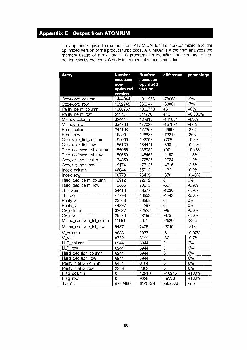
Appendix E Output from ATOMIUM

This appendix gives the output from ATOMIUM for the non-optimized and theoptimized version of the product turbo code. ATOMIUM is a tool that analyzes thememory usage of array data in C programs an identifies the memory relatedbottlenecks by means of C code instrumentation and simulation

Array Number Number difference percentageaccesses accessesnon- optimizedoptimized versionversion

Codeword column 1444344 1366276 -78068 -5%Codeword row 1032745 963944 -68801 -7%Parity perm column 1006767 1006773 +6 +0%Parity_perm row 511757 511770 +13 +0.003%Metrics column 324444 182810 -141634 -4.3%Metrics row 334700 177029 -157671 -47%Perm column 244168 177268 -66900 -27%Perm row 199904 126688 -73216 -36%Codeword list column 192000 192708 +708 +0.3%Codeword list row 155139 154441 -698 -0.45%Tmp codewrd list column 186088 186989 +901 +0.48%Tmp codewrd list row 150660 148468 -2192 -1.5%Codewrd sqn column 174850 172826 -2024 -1.2%Codewrd sqn row 181741 177125 -4616 -2.5%Index column 66044 65912 -132 -0.2%Index row 76779 76409 -370 -0.48%Hard dec _perm column 72912 72912 0 0%Hard dec _perm row 70866 70215 -651 -0.9%LL column 54413 53377 -1036 -1.9%LL row 47798 46553 -1243 -2.6%Parity_ x 23568 23568 0 0%Parity v 44297 44297 0 0%Cv column 32627 32529 -98 -0.3%Cv row 28573 28195 -378 -1.3%Metric_codewrd_lsLcolmn 11691 9071 -2620 -29%Metric_codewrd_lsLrow 9457 7408 -2049 -21%V column 8883 8877 -6 -0.07%V row 8762 8699 -62 -0.7%LLR column 6944 6944 0 0%LLR row 6944 6944 0 0%Hard decision column 6944 6944 0 0%Hard decision row 6944 6944 0 0%Parity matrix column 6404 6404 0 0%Parity matrix row 2303 2303 0 0%Flaq column 0 10916 +10916 +100%Flaq row 0 9338 +9338 +100%TOTAL 6732460 6149874 -582583 -9%

66

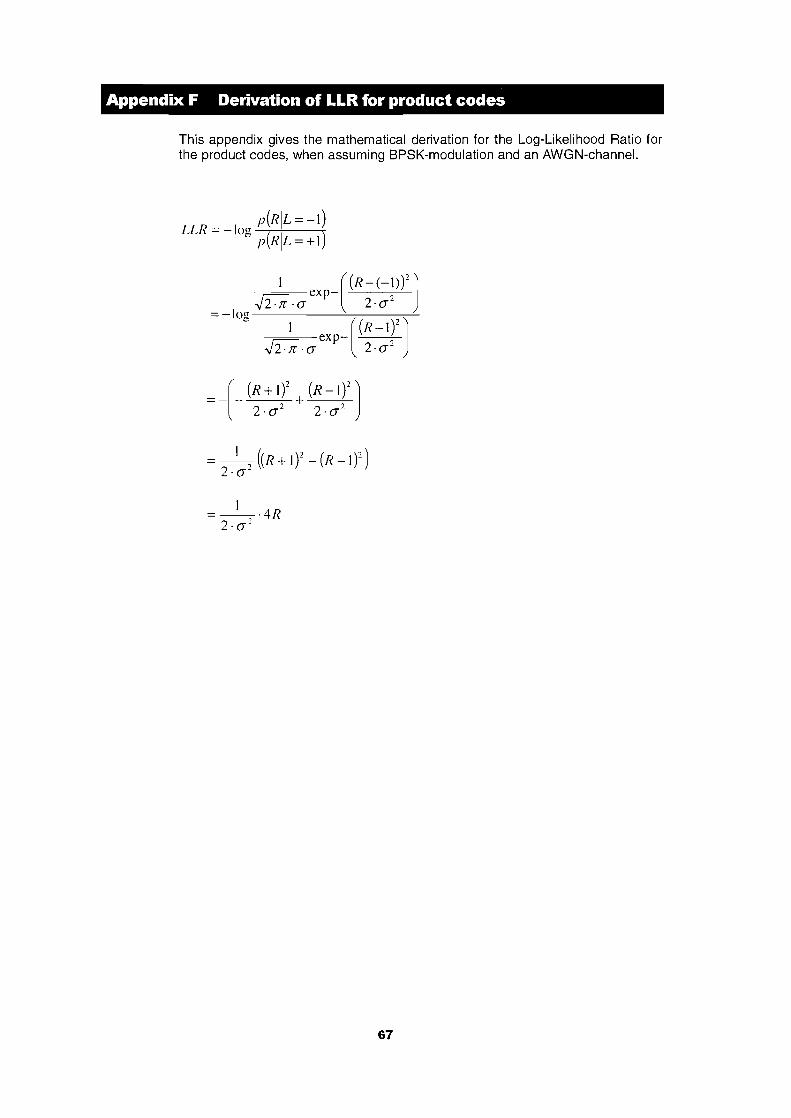
Appendix F Derivation of LLR for product codes

This appendix gives the mathematical derivation for the Log-Likelihood Ratio forthe product codes, when assuming BPSK-modulation and an AWGN-channel.

p(RIL =-I)LLR = -log p(RIL = +1)

1 [(R-(-l))"]exp-~.~ 2·~2=-lo(T-----'----,,---~

b 1 [(R-I)"]exp- 0

~.~ 2·~-

=_1_, ((R+l)"-(R-I)")2· ~-

1=--·4R

2. ~2

67

Appendix G Sorting algorithms

For the product code, a sorting algorithm is needed. This appendix gives twodifferent types of sorting algorithms in C code.

G.1. Bubble sort

void Bubble_Sort (float list[N]){/* this algorithm sorts a list by putting the (n+1)th element at the right place between the nalready sorted elements */

int j,k;float temp;

for (j=O;j<N-1 ;j++)for (k=O;k<N-1-j;k++)

if (Iist[k] > list[k+1]){

temp = list[j];list[j] = Iist[k];list[k] = temp;

}

G.2. Shell's law

void Shell (float list[N]){/* this algorithm sorts a list of for example 16 numbers nloo.n,6 by first sorting each of the 8groups of 2 (n" ns), (n2, ns), 00' ,(ns, n,6); then sort each of the 4 groups of 4 (n" ns, ns, n,3)• .•• •(n4,ns, n'2, n,6); next sort 2 groups of 8 records and finally sort the whole list. */

int j.k, inc;float temp;

inc = 1;

/* determine the starting increment */do{

inc *=3 ;inc++} while (inc <= N);

/* loop over partial sorts */do{

inc /= 3;for (j-inc+1;j<=n;j++)

{temp = a[j];k =j;while (a[k-inc] > temp)

{ark] = a[k-inc];k -= inc;if (k <= inc) break;}

ark] = temp;}

}while (inc> 1);

68