eindhoven university of technology master combined
TRANSCRIPT

Eindhoven University of Technology
MASTER
Combined simulation of district heating and electrical power networks
Klinkel, Kevin G.
Award date:2020
Link to publication
DisclaimerThis document contains a student thesis (bachelor's or master's), as authored by a student at Eindhoven University of Technology. Studenttheses are made available in the TU/e repository upon obtaining the required degree. The grade received is not published on the documentas presented in the repository. The required complexity or quality of research of student theses may vary by program, and the requiredminimum study period may vary in duration.
General rightsCopyright and moral rights for the publications made accessible in the public portal are retained by the authors and/or other copyright ownersand it is a condition of accessing publications that users recognise and abide by the legal requirements associated with these rights.
• Users may download and print one copy of any publication from the public portal for the purpose of private study or research. • You may not further distribute the material or use it for any profit-making activity or commercial gain
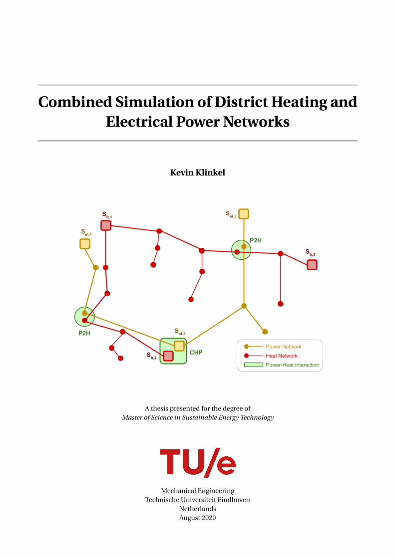
Combined Simulation of District Heating andElectrical Power Networks
Kevin Klinkel
Sel,1
Sel,3
Sel,2
Sh,1
Sh,2
Sh,3
P2H
CHP
P2H
Heat Network
Power Network
Power-Heat Interaction
A thesis presented for the degree ofMaster of Science in Sustainable Energy Technology
Mechanical EngineeringTechnische Universiteit Eindhoven
NetherlandsAugust 2020


February 21, 2020
Declaration concerning the TU/e Code of Scientific Conduct for the Master’s thesis I have read the TU/e Code of Scientific Conducti. I hereby declare that my Master’s thesis has been carried out in accordance with the rules of the TU/e Code of Scientific Conduct Date …………………………………………………..………….. Name …………………………………………………..………….. ID-number …………………………………………………..………….. Signature …………………………………………………..………….. Submit the signed declaration to the student administration of your department. i See: https://www.tue.nl/en/our-university/about-the-university/organization/integrity/scientific-integrity/ The Netherlands Code of Conduct for Scientific Integrity, endorsed by 6 umbrella organizations, including the VSNU, can be found
here also. More information about scientific integrity is published on the websites of TU/e and VSNU
Aug 18, 2020
Kevin Klinkel
1508105


Abstract
Decarbonization is causing further electrification of energy systems which traditionally depended on fossilfuels. This is leading to increased interactions between energy systems, especially those related to the heatand electricity sectors. Conventionally energy networks have been simulated as separate, independent sys-tems, but the integration of more points of interaction between different energy networks means that theyare becoming more deeply coupled and cannot be considered as separate. This thesis aims to investigatewhat differences arise when a coupled heat and electricity network is simulated in an integrated approachwith a combined heat-electric network model compared to simulating the networks independently, usingconventional load flow techniques.
A heat network model is implemented for performing load flow simulation of district heating networks,and the commercial software SAInt is employed to handle AC power flow simulation of electrical networks.Heat-electric coupling components such as heat pumps and CHP plants are modeled using the energy hubconcept which encapsulates interactions between the networks at discrete points. A combined heat-electricnetwork load flow solver is then created which uses energy hubs to facilitate sequential information ex-change between the heat and electricity network simulation tools in an iterative process. Finally an inves-tigation is carried out which simulates a coupled heat and electricity network in an integrated approachas well as simulating both systems independently. Results indicated that losses from one network wereneglected in the opposing network when the simulations were not integrated together, which caused thetotal network supply power to differ depending on which simulation was run. This discrepancy in the netsupply and demand affected how power was allocated among the participating power producers in bothsystems which had a meaningful effect on the different simulation outcomes. The combined heat-electricsimulation found a more balanced load flow solution that the individual simulations were only able to ap-proximate.
Keywords:
decarbonization, district heating network, combined heat and electricity simulation, energy hub, load flow


For my son Calem
... despite his best efforts, I still finished

Acknowledgments
This master’s thesis is the product of two years of very hard and rewarding work which was made possible byEIT InnoEnergy and the MSc SELECT program (Master’s in Environomical Pathways for Sustainable EnergySystems). I have the coordinators of the MSc SELECT program to thank for accepting me into the program,especially César Valderrama who was the coordinator of my first year at Universitat Politècnica de Catalunya(UPC) in Barcelona, and Han van Kasteren who coordinated the second year program at the TechnischeUniversiteit Eindhoven (TU/e), here in the Netherlands.
The topic of this thesis project found its way to me through serendipitous means, and I ultimately have Dr.Kwabena Pambour and Dr. Carlo Brancucci to thank for bringing me onto this project with encoord®GmbH.I would especially like to thank Dr. Kwabena Pambour for guiding me through the many twists and turnsthat riddle the journey of creating an energy system simulation model. His patience, reliability, and will-ingness to help are without a doubt a main contributor to my success in completing this project. He hasopened my eyes to the devilish beauty of network modeling, and I don’t think I will ever look at the worldthe same again.
I would like to express my gratitude to dr.ir. Camilo Rindt who directs the Sustainable Energy Technologygroup within TU/e. His guidance has always been reliable and succinct, and he encouraged without a doubtthat I strive to produce high quality work that I would be proud of.
Finally, I would like the express my dearest thanks to my parents who brought me up so that I would endup here today, my wife Kara who supports me immeasurably and always believes in me, and my son Calemwho keeps me going.
i

Contents
List of Figures iv
List of Tables v
Nomenclature vi
1 Introduction 11.1 Background and Motivation . . . . . . . . . . . . . . . . . . . . . . . . . . . . . . . . . . . . . . . . 11.2 Heat and Electricity Systems . . . . . . . . . . . . . . . . . . . . . . . . . . . . . . . . . . . . . . . 3
1.2.1 District Heating Systems . . . . . . . . . . . . . . . . . . . . . . . . . . . . . . . . . . . . . . 31.2.2 Electricity Systems . . . . . . . . . . . . . . . . . . . . . . . . . . . . . . . . . . . . . . . . . 41.2.3 Interaction Points Between Electricity and Heat Networks . . . . . . . . . . . . . . . . . . 4
1.3 Modeling Review . . . . . . . . . . . . . . . . . . . . . . . . . . . . . . . . . . . . . . . . . . . . . . 61.3.1 Energy Network Simulation . . . . . . . . . . . . . . . . . . . . . . . . . . . . . . . . . . . . 61.3.2 Combined Network Modeling Techniques . . . . . . . . . . . . . . . . . . . . . . . . . . . 7
1.4 Gap in the Literature . . . . . . . . . . . . . . . . . . . . . . . . . . . . . . . . . . . . . . . . . . . . 91.5 Research Question . . . . . . . . . . . . . . . . . . . . . . . . . . . . . . . . . . . . . . . . . . . . . 91.6 Thesis Outline . . . . . . . . . . . . . . . . . . . . . . . . . . . . . . . . . . . . . . . . . . . . . . . . 10
2 District Heating Network Model 112.1 Fundamental Structure of a District Heating Network . . . . . . . . . . . . . . . . . . . . . . . . 11
2.1.1 Example Heat Network . . . . . . . . . . . . . . . . . . . . . . . . . . . . . . . . . . . . . . . 112.2 Network Topology . . . . . . . . . . . . . . . . . . . . . . . . . . . . . . . . . . . . . . . . . . . . . . 12
2.2.1 Radial and Meshed Network Topologies . . . . . . . . . . . . . . . . . . . . . . . . . . . . . 122.2.2 Energy Network as a Directed Graph . . . . . . . . . . . . . . . . . . . . . . . . . . . . . . 13
2.3 Load Flow Analysis of Energy Networks . . . . . . . . . . . . . . . . . . . . . . . . . . . . . . . . . 142.4 Hydraulic Equations . . . . . . . . . . . . . . . . . . . . . . . . . . . . . . . . . . . . . . . . . . . . 14
2.4.1 Continuity of Flow . . . . . . . . . . . . . . . . . . . . . . . . . . . . . . . . . . . . . . . . . 142.4.2 Pipe Head Loss . . . . . . . . . . . . . . . . . . . . . . . . . . . . . . . . . . . . . . . . . . . 15
2.5 Thermal Equations . . . . . . . . . . . . . . . . . . . . . . . . . . . . . . . . . . . . . . . . . . . . . 162.5.1 Heat Power . . . . . . . . . . . . . . . . . . . . . . . . . . . . . . . . . . . . . . . . . . . . . . 162.5.2 Pipe Temperature Drop . . . . . . . . . . . . . . . . . . . . . . . . . . . . . . . . . . . . . . 162.5.3 Temperature Mixing . . . . . . . . . . . . . . . . . . . . . . . . . . . . . . . . . . . . . . . . 17
2.6 District Heating Network Solution . . . . . . . . . . . . . . . . . . . . . . . . . . . . . . . . . . . . 172.6.1 Hydraulic Solution . . . . . . . . . . . . . . . . . . . . . . . . . . . . . . . . . . . . . . . . . 172.6.2 Hydraulic-Thermal Solution . . . . . . . . . . . . . . . . . . . . . . . . . . . . . . . . . . . 182.6.3 Distributed Slack Model . . . . . . . . . . . . . . . . . . . . . . . . . . . . . . . . . . . . . . 182.6.4 Heat Network Solver . . . . . . . . . . . . . . . . . . . . . . . . . . . . . . . . . . . . . . . . 19
2.7 Validation of District Heating Model . . . . . . . . . . . . . . . . . . . . . . . . . . . . . . . . . . . 202.7.1 Barry Island Heat Network . . . . . . . . . . . . . . . . . . . . . . . . . . . . . . . . . . . . 202.7.2 Comparison to Benchmark Simulation . . . . . . . . . . . . . . . . . . . . . . . . . . . . . 22
3 Electricity Network Model 253.1 Power Flow Overview . . . . . . . . . . . . . . . . . . . . . . . . . . . . . . . . . . . . . . . . . . . . 25
ii

Contents
3.1.1 Power Flow Equations . . . . . . . . . . . . . . . . . . . . . . . . . . . . . . . . . . . . . . . 263.1.2 Per-Unit System . . . . . . . . . . . . . . . . . . . . . . . . . . . . . . . . . . . . . . . . . . . 263.1.3 Ybus Admittance Matrix . . . . . . . . . . . . . . . . . . . . . . . . . . . . . . . . . . . . . . 263.1.4 Generic Branch Model (π-model) . . . . . . . . . . . . . . . . . . . . . . . . . . . . . . . . 26
3.2 AC Power Flow Solution . . . . . . . . . . . . . . . . . . . . . . . . . . . . . . . . . . . . . . . . . . 27
4 Heat-Electric Combined Model 284.1 Network Coupling Components . . . . . . . . . . . . . . . . . . . . . . . . . . . . . . . . . . . . . 28
4.1.1 Heat Pumps . . . . . . . . . . . . . . . . . . . . . . . . . . . . . . . . . . . . . . . . . . . . . 284.1.2 Electric Boilers . . . . . . . . . . . . . . . . . . . . . . . . . . . . . . . . . . . . . . . . . . . 294.1.3 Combined Heat and Power Plants . . . . . . . . . . . . . . . . . . . . . . . . . . . . . . . . 294.1.4 Circulation Pumps . . . . . . . . . . . . . . . . . . . . . . . . . . . . . . . . . . . . . . . . . 30
4.2 Energy Hubs . . . . . . . . . . . . . . . . . . . . . . . . . . . . . . . . . . . . . . . . . . . . . . . . . 304.3 Heat Electric Combined Solver . . . . . . . . . . . . . . . . . . . . . . . . . . . . . . . . . . . . . . 31
5 Case Study 335.1 Strategy of the Investigation . . . . . . . . . . . . . . . . . . . . . . . . . . . . . . . . . . . . . . . . 335.2 Network Descriptions . . . . . . . . . . . . . . . . . . . . . . . . . . . . . . . . . . . . . . . . . . . 33
5.2.1 Heat Network . . . . . . . . . . . . . . . . . . . . . . . . . . . . . . . . . . . . . . . . . . . . 335.2.2 Electric Network . . . . . . . . . . . . . . . . . . . . . . . . . . . . . . . . . . . . . . . . . . 345.2.3 Combined Heat-Electric Network . . . . . . . . . . . . . . . . . . . . . . . . . . . . . . . . 345.2.4 Slack Participation . . . . . . . . . . . . . . . . . . . . . . . . . . . . . . . . . . . . . . . . . 355.2.5 Initial Setpoints . . . . . . . . . . . . . . . . . . . . . . . . . . . . . . . . . . . . . . . . . . . 35
5.3 Results . . . . . . . . . . . . . . . . . . . . . . . . . . . . . . . . . . . . . . . . . . . . . . . . . . . . 365.3.1 Combined Heat-Electric Solution . . . . . . . . . . . . . . . . . . . . . . . . . . . . . . . . 365.3.2 Combined Solution Compared to Individual Solutions . . . . . . . . . . . . . . . . . . . . 365.3.3 Network-Level Results . . . . . . . . . . . . . . . . . . . . . . . . . . . . . . . . . . . . . . . 38
5.4 Discussion . . . . . . . . . . . . . . . . . . . . . . . . . . . . . . . . . . . . . . . . . . . . . . . . . . 405.5 Limitations of the Study . . . . . . . . . . . . . . . . . . . . . . . . . . . . . . . . . . . . . . . . . . 41
6 Conclusion 43
Bibliography I
Appendix A Newton-Raphson Method V
Appendix B Linearizations of Heat Network Equations VII
Appendix C Barry Island Network Parameters X
Appendix D Case Study Network Parameters XII
Appendix E Case Study Load Flow Results XV
iii CONTENTS

List of Figures
1.1 GHG emissions by economic sector . . . . . . . . . . . . . . . . . . . . . . . . . . . . . . . . . . . 11.2 Origins of heat supply for residential and service sector buildings . . . . . . . . . . . . . . . . . 21.3 Simplified diagram of a typical district heating system . . . . . . . . . . . . . . . . . . . . . . . . 31.4 Simplified diagram of a typical electrical system . . . . . . . . . . . . . . . . . . . . . . . . . . . . 51.5 Coupling points between power and heat systems . . . . . . . . . . . . . . . . . . . . . . . . . . 61.6 Energy conversions in a multi-carrier energy network . . . . . . . . . . . . . . . . . . . . . . . . 71.7 Energy hub concept . . . . . . . . . . . . . . . . . . . . . . . . . . . . . . . . . . . . . . . . . . . . 81.8 Convergence characteristics of decomposed and integrated models . . . . . . . . . . . . . . . . 8
2.1 Radial heat network branch with N load nodes . . . . . . . . . . . . . . . . . . . . . . . . . . . . . 122.2 Simple meshed heat network with 2 customers . . . . . . . . . . . . . . . . . . . . . . . . . . . . 122.3 Main network topologies . . . . . . . . . . . . . . . . . . . . . . . . . . . . . . . . . . . . . . . . . 132.4 Incidence matrix of directed graph . . . . . . . . . . . . . . . . . . . . . . . . . . . . . . . . . . . . 132.5 Supply and return network symmetry . . . . . . . . . . . . . . . . . . . . . . . . . . . . . . . . . . 152.6 Heat Network Solver Flowchart . . . . . . . . . . . . . . . . . . . . . . . . . . . . . . . . . . . . . . 202.7 Barry Island district heating network . . . . . . . . . . . . . . . . . . . . . . . . . . . . . . . . . . 21
3.1 Simple example of electrical network with one generator and two loads . . . . . . . . . . . . . 253.2 Generic branch model (π-circuit) used in SAInt electrical networks . . . . . . . . . . . . . . . . 27
4.1 CHP operating ranges . . . . . . . . . . . . . . . . . . . . . . . . . . . . . . . . . . . . . . . . . . . 294.2 Energy hub implementation of a heat pump . . . . . . . . . . . . . . . . . . . . . . . . . . . . . . 314.3 Heat Electric Combined Solver Flowchart . . . . . . . . . . . . . . . . . . . . . . . . . . . . . . . . 32
5.1 Heat network model used for the case study . . . . . . . . . . . . . . . . . . . . . . . . . . . . . . 345.2 Electric network model used for the case study . . . . . . . . . . . . . . . . . . . . . . . . . . . . 345.3 Combined Heat-Electric network model used for the case study . . . . . . . . . . . . . . . . . . 355.4 Iterative convergence of the Heat-Electric combined solver . . . . . . . . . . . . . . . . . . . . . 365.5 Heat and electric power results simulation comparison . . . . . . . . . . . . . . . . . . . . . . . 375.6 Absolute and relative differences between combined and individual simulation results . . . . 385.7 Total network differences between combined and individual simulation results . . . . . . . . . 395.8 Absolute and relative differences of heat and electrical power allocation . . . . . . . . . . . . . 39
A.1 Newton-Raphson method: Linearization about an operating point . . . . . . . . . . . . . . . . VI
C.1 Barry Island district heating network . . . . . . . . . . . . . . . . . . . . . . . . . . . . . . . . . . X
iv

List of Tables
2.1 Node types in Energy Systems . . . . . . . . . . . . . . . . . . . . . . . . . . . . . . . . . . . . . . 142.2 Barry Island network parameters . . . . . . . . . . . . . . . . . . . . . . . . . . . . . . . . . . . . . 212.3 Barry Island heat loads . . . . . . . . . . . . . . . . . . . . . . . . . . . . . . . . . . . . . . . . . . . 212.4 Mass flow results validated . . . . . . . . . . . . . . . . . . . . . . . . . . . . . . . . . . . . . . . . 222.5 Node temperature results validated . . . . . . . . . . . . . . . . . . . . . . . . . . . . . . . . . . . 232.6 Heat power calculated for Barry Islanc source 2 (slack node) . . . . . . . . . . . . . . . . . . . . 23
5.1 Heat-Electric network coupling points . . . . . . . . . . . . . . . . . . . . . . . . . . . . . . . . . 355.2 Distributed slack participation among power producers . . . . . . . . . . . . . . . . . . . . . . . 355.3 Coupling components initial power setpoints . . . . . . . . . . . . . . . . . . . . . . . . . . . . . 365.4 Power results of coupling components for combined and individual simulations . . . . . . . . 375.5 Total network supply power for combined and individual simulations . . . . . . . . . . . . . . . 385.6 Network-level load flow results . . . . . . . . . . . . . . . . . . . . . . . . . . . . . . . . . . . . . . 38
C.1 Barry Island network parameters . . . . . . . . . . . . . . . . . . . . . . . . . . . . . . . . . . . . . XC.2 Barry Island heat network pipe parameter . . . . . . . . . . . . . . . . . . . . . . . . . . . . . . . XI
D.1 Case study heat pipe parameters . . . . . . . . . . . . . . . . . . . . . . . . . . . . . . . . . . . . . XIID.2 Case study heat network parameters . . . . . . . . . . . . . . . . . . . . . . . . . . . . . . . . . . . XIIID.3 Case study heat loads . . . . . . . . . . . . . . . . . . . . . . . . . . . . . . . . . . . . . . . . . . . . XIIID.4 Case study electric line parameters . . . . . . . . . . . . . . . . . . . . . . . . . . . . . . . . . . . XIIID.5 Case study electric network parameters . . . . . . . . . . . . . . . . . . . . . . . . . . . . . . . . . XIVD.6 Case study electric loads . . . . . . . . . . . . . . . . . . . . . . . . . . . . . . . . . . . . . . . . . . XIV
E.1 Case study heat node results . . . . . . . . . . . . . . . . . . . . . . . . . . . . . . . . . . . . . . . XVE.2 Case study heat pipe flows . . . . . . . . . . . . . . . . . . . . . . . . . . . . . . . . . . . . . . . . . XVIE.3 Case study electric bus results . . . . . . . . . . . . . . . . . . . . . . . . . . . . . . . . . . . . . . XVIIE.4 Case study electric line currents . . . . . . . . . . . . . . . . . . . . . . . . . . . . . . . . . . . . . XVIII
v

Nomenclature
Abbreviations
CHEsim Combined Heat-Electric Simulation
CHP Combined Heat and Power
DH District Heating
DHC District Heating and Cooling
DHW Domestic Hot Water
DSM Demand-Side Management
EB Electric Boiler
ENET Electric Network
ERH Electric Resistor Heater
Esim Electric-only Simulation
GHG Greenhouse Gases
HNET Heat Network
HP Heat Pump
Hsim Heat-only Simulation
HV High Voltage
HX Heat Exchanger
IES Integrated Energy System
IHPD Integrated Heat & Power Dispatch
KCL Kirchoff’s Current Law
KVL Kirchoff’s Voltage Law
LHS Left-Hand Side
LTDH Low Temperature District Heating
LV Low Voltage
MCEN Multi-Carrier Energy Network
MV Medium Voltage
P2G Power-to-Gas
P2H Power-to-Heat
RE Renewable Energy
vi

Nomenclature
RHS Right-hand side
TES Thermal Energy Storage
TSO Transmission System Operator
VF-CT Variable Flow, Constant Temperature
VRES Variable Renewable Energy Sources
Subscripts and Superscripts
k+1 Next Iteration
k Iteration k
SP Set Point
i Inlet
n Node
o Outlet
p Pipe
q Heat External
r q Heat External Return
r Heat Network Return
sq Heat External Supply
s Heat Network Supply
Electricity Network Variables
δ Voltage Angle °
θ Phase Angle °
B Susceptance Ω−1
F Frequency Hz
G Conductance Ω−1
I Current A
P Active (real) Power W
p.f. Power Factor −Q Reactive (imaginary) Power VAr
R Resistance Ω
S Apparent (complex) Power VA
V Voltage V
X Reactance Ω
Y Admittance Ω−1
Z Impedance Ω
Heat Network Variables
m Mass Flow Rate kg/s
vii NOMENCLATURE

Nomenclature
µ Dynamic Viscosity Pa · s
ν kinematic Viscosity m/s2
Φ Heat Power Flow W
Ψ Relative Temperature Attenuation Factor −ρ Density kg/m3
cp Heat Capacity J/kg ·K
h Fluid Head m
K Pipe Flow Resistance Coefficient −P Pressure Pa
T Temperature C, K
T ′ Excess Temperature (above ambient) C, K
Miscellaneous
βi Participation Factor (for distributed slack) −
NOMENCLATURE viii

Chapter 1
Introduction
1.1 Background and Motivation
Because of the effects of climate change, there is a global need to reduce green house gas (GHG) emissionsto mitigate a slate of adverse effects to human and ecological well-being. In an effort to combat this, manycountries have set goals to reduce GHG emissions by increasing the share of renewable energy sources (RES)and improving efficiencies, among other measures. The European Commission for example set targets toreduce GHG emissions in power generation, aiming to decarbonize 57–65% by 2030 and 96–99% by 2050[41], noting that the power system would have to undergo structural change in order to do so. The roadmapalso indicates that renewable heating and cooling are vital to decarbonization. Low-carbon and locally-produced energy sources, as well as heat pumps, storage heaters, and district heating (DH) systems areindispensible to this transformation.
Other Energy9.6%
Industry21.0%
Transport14.0%Buildings6.4%
Electricity and Heat25.0%
AFOLU24.0%
Figure 1.1: GHG emissions by economic sector (data from IPCC [7])
The electricity and heating sector is one of the largest contributors to GHG emissions, with a share of 25%of all emissions in 2010 according to a 2014 assessment by the Intergovernmental Panel on Climate Change(IPCC) [7]. The electricity sector is seeing an increase in the penetration of renewable energy technologies.However, many renewable energy sources, particularly wind and solar, are variable and intermittent bynature and cannot always match the instantaneous demand. If there is not enough capacity for energystorage or load shifting then this variability of supply creates problems in the power balance. Times inwhich there is a deficit in supply means power from dispatchable sources (often fossil fuels) must make upfor the difference. Times in which there is an excess of supply means energy capture will be curtailed andthus renewable energy generation potential is wasted. With increasing shares of variable renewable energy(VRE) there is a need for energy storage in order to ensure that excess renewable energy is captured and
1

1.1. Background and Motivation
can be used at times when production is low. However very large amounts of electricity cannot be storedcheaply, so alternate approaches must be taken to ensure successful integration of volatile renewable energysources.
The heat sector was historically almost completely dependent on burning fuels in order to provide usefulheat, with much of these fuels being fossil fuel origin. Although the mix of heat supply has diversified, themajority of heat for residential and service sector buildings is provided by fossil fuels (see Figure 1.2). Forthe heat sector to decarbonize, the primary energy sources will have to be renewable in origin, meaningbiomass and biofuels for fuel-based combustion, solar thermal or geothermal energy when possible, andelectrical heating powered from renewable electricity.
Coal and Coal Products3.0%Petroleum Products17.0%
Natural Gas44.0%
District Heating13.0%
Electricity12.0%
Combustible Renewables10.0%
Solar/Wind/Other1.0%
Figure 1.2: Origins of heat supply for residential and service sector buildings in EU27countries during 2010 (data from [10])
Power-to-heat (P2H) technologies use electricity to produce heat, and can come in a couple different forms.Electric boilers (EB) and electric heaters convert electricity directly into heat by running current through aresistor which becomes hot. Heat pumps (HP) on the other hand use electricity to run a thermodynamiccycle which moves heat from a cold heat source to a warmer heat sink, and therefore can be used for heatingand/or cooling needs. Since many renewable energy sources produce electricity directly (like wind, solarPV, and hydropower) P2H technologies are a great carbon-free option for meeting thermal needs.
P2H can provide simultaneous benefits to both the power and heat sectors: while it can contribute to de-carbinization of the heat sector, it can also add flexibility options to the electricity sector [58]. Heatingand cooling demands can often be shifted in time because of thermal inertia, which means P2H can offerload-shifting potential as a demand-side management (DSM) option to help the electricity sector cope withpower balance mismatches. When thermal energy storage (TES) is used with P2H there is a large capac-ity to add flexibility to the electrical demand. In a study of DSM for increased power flexibility applied toHelsinki, Finland, Salpakari et al. [43] found that for a scheme providing 50% of all electricity through self-consumption of variable renewable electricity, P2H in combination with thermal storage could absorb allsurplus electricity production, eliminating the need for curtailment. A study by Lund et al. [32] analyzeddifferent schemes for using heat pumps and TES to increase the share of wind power in Denmark.
Thermal energy storage also has the advantage of cost. Large-scale battery storage is significantly moreexpensive than thermal energy storage, and the materials used in batteries have damaging ecological foot-prints. TES on the other hand is one of the most inexpensive forms of energy storage and can be easy toimplement. In its simplest form TES is essentially a hot water tank. Other forms include storing thermalenergy in the ground or naturally existing aquifers by pumping heated or cooled water through boreholesin the ground. These can also be used as long-term seasonal storage. The simplicity and cost of TES makeit a great option for storing excess electrical energy from VREs when P2H technologies are used.
It is clear that the heat sector and electricity sector can offer each other mutual benefits through the use ofP2H technologies. Heat production can be decarbonized by utilizing renewable electricity, and the electric-
CHAPTER 1. INTRODUCTION 2

1.2. Heat and Electricity Systems
ity sector can gain flexibility through the load shifting and potential for energy storage offered by the heatsector. Next the structure and operation of district heating and electrical systems are described.
1.2 Heat and Electricity Systems
1.2.1 District Heating Systems
District heating (DH) networks use a network of insulated supply and return pipes to deliver heat from heatproducers to end consumers, using water as the heat carrying medium. The heat can be generated by oneor multiple producers, and is generally delivered to a larger number of consumers. The supply lines carrywater at a higher temperature, typically around 70°C to 120 °C. The return line then carries water after heathas been extracted, at temperatures around 30 °C to 50 °C, so it can be brought back to the heat producers.The heat is supplied to the consumer by way of a heat exchanger substation [21] which provides a hydraulicseparation between the main DH water network and the subsystem. Electrically-driven circulation pumpsare located at the heat production plants and sometimes also in substations. These provide the pressureneeded for the water to flow through the piping system and to maintain a pressure differece between thesupply and return lines [30].
Figure 1.3: Simplified diagram of a typical district heating system (figure from [30])
District heating systems offer several advantages compared to all consumers having their own heating sys-tems [56]:
• Higher energy efficiency of the overall system
• Lower cost of heat to costumers
• Maintenance and monitoring are managed by the heat utilities. Customers do not have to maintaintheir own boiler or heating unit.
• Ability to use local renewable energy resources
• Waste heat can be recovered and fed into the DH network, which allows producers of waste heat tosell it.
Producers of heat traditionally were thermal power plants or combined heat and power (CHP) plants, butnewer generation DH networks can incorporate heat from various other sources, including flue gas conden-sation, solar thermal, sewage, industrial waste heat from cooling or lubrication fluid, and other processes
3 CHAPTER 1. INTRODUCTION

1.2. Heat and Electricity Systems
that produce heat or waste heat [39]. The heat is generally consumed for use in space heating (SH) anddomestic hot water (DHW). Often DH systems deliver to residential neighborhoods, apartment buildings,schools and university campuses, medical facilities, and military bases.
The oldest, 1st generation DH networks were established in the US in the late 1870’s and used steam asan energy carrier.1 In the 1930’s 2nd generation systems switched to pressurized water above 100°C. Sincethe 1980’s, 3rd generation DH networks have focused on utilizing lower temperatures, prefabricated andpre-insulated pipes, and material-lean installation. Newer 4th generation systems aim to use further lowertemperatures, assembly-oriented components, and more flexible materials [29]. 4th generation DH tech-nology can also take advantage of multi-energy cascades in both supply and demand. An example of suchan energy cascade is connecting the return line of a higher-temperature system to the supply line of a low-temperature heating system, for example a radiator return line can feed into the low temperature floor heat-ing supply line [39].
DH networks often incorporate thermal energy storage units for a variety of reasons like helping meet peakdemand or dealing with ramping times. These can take many forms, inlcuding water tanks, buried pits,borehole, or aquifer storage. In fact the actual network itself - including the pipes and ground the pipes areburied in - has an appreciable amount of thermal inertia which can be utilized. One study by Zheng et al.[62] demonstrated that utilizing the thermal inertia of the district heating network was an effective energy-saving method for improving the operational flexibility of CHP plants, which promoted integration of windpower in an integrated heat and power dispatch (IHPD) system.
1.2.2 Electricity Systems
The electrical power system consists mainly of components related to generation, transmission, distribu-tion, and consumption of electricity. The electrical network is divided broadly into transmission and dis-tribution, depending on the functionality, voltage level, and spanned area [24, 48]. A generator which pro-duces power at 11-35 kV for example injects power into the high voltage (HV) transmission system by step-ping up the voltage through a transformer to around 220-1000 kV [55]. The transmission system connectsareas hundreds or thousands of kilometers apart with electrical lines and transports bulk power betweenpower plants and load centers (usually metropolitan areas). The power from the transmission system isstepped down by transformers into the medium voltage (MV) distribution system, usually around 2-35 kV,before being brought near its final destination where the voltage is again stepped down to around 220-380V for use in the low voltage (LV) service area (usually a whole city) [55] where the conductors are primarilyunderground insulated cables.
The transmission and distribution systems differ in structure and AC characteristics. The transmission sys-tem is typically more meshed in topology so that the built-in redundancy provides higher reliability, and thepower delivered in each of the 3 phases is balanced. The distribution system on the other hand is generallya branched topology which operates radially, and the load supplied by each phase could be imbalanced[24, 30].
While conventional generation happens in bulk at larger power plants, more recently the landscape is shift-ing towards more and more distributed power generation, especially with the broad deployment of solar PV.Loads are also becoming more responsive as computerized control systems and informatics become inte-grated. The response to these changes is rapidly evolving with bi-directional power flows and distributionnetworks incorporating more meshed topology than before [55].
1.2.3 Interaction Points Between Electricity and Heat Networks
Future power systems will see an increase in district heating and cooling networks in an effort to decar-bonize the heat sector and incorporate more renewable primary energy sources. There are many opportu-nities for innovation and increased efficiency in power-to-heat systems. As mentioned, P2H technologies
1Interestingly, the original purpose of delivering steam was not for heating, but for generating electricity in the buidlings con-nected to the steam network [56]. When electrical networks appeared a decade later the purpose of the steam networks changedto be used as a source for heating.
CHAPTER 1. INTRODUCTION 4

1.2. Heat and Electricity Systems
Figure 1.4: Simplified diagram of a typical electrical system (figure from [55])
used together with DH systems can provide added flexibility that is necessary for incorporating variablerenewable energy sources. There are several possible points of interaction between the electrical grid anddistrict heating systems, such as:
• CHP and polygeneration plants
• Centralized heat pumps
• Centralized electric boilers
• Centralized heat storage
• Circulation pumps
In these points of interaction, excess power can be used to produce heat in the district heating network,which can then be either consumed directly or stored in thermal energy storage units. A diagram that showssimply the main interaction points between the power and heat networks is shown in Figure 1.5.
The presence of these interaction points, combined with the fact that thermal energy storage cost is lowcompared to electrical storage cost, makes it increasingly attractive to plan and operate power and heatnetworks together [6]. A coordinated effort between power and heat network operation could contribute
5 CHAPTER 1. INTRODUCTION

1.3. Modeling Review
Figure 1.5: Coupling points between power and heat systems (figure from [6])
simultaneously toward decarbonizing the heating sector and providing more flexibility needed for inter-mittent renewable energy resources.
As Connolly et al. [10] mentions, energy system modeling tools are typically made for the electricity sector,and the potential benefits of district heating systems tend to be overlooked. Local conditions usually need tobe considered when assessing the potential for DH networks, which is typically not the case in internationalenergy simulation tools. If modeling tools are used which do not take into account the interaction betweenboth networks then it is important to understand what limitations these tools have compared to a holisticapproach which considers both systems as an integrated whole.
1.3 Modeling Review
1.3.1 Energy Network Simulation
The most fundamenal analysis of energy networks is load flow or power flow simulation, which finds thesteady-state transport of energy through the system. In electrical systems the AC power flow finds the volt-ages and power injections at each bus, and the real and reactive power flows through each branch [55, 37].The network power flow is computed by treating the network as a circuit and applying Ohm’s law and Kir-choff’s laws accordingly, with the voltages and currents being represented by complex phasors. Similar loadflow analysis is performed for district heating networks which determines the water flow rates through thenetwork and the temperatures and pressures at each node. The hydraulic aspect of DH load flow uses equa-tions similar to the Kirchoff’s laws in the electrical power flow model for continuity of flow through a nodeand pressure drop around a loop [38, 40, 30, 19]. Load flow analysis can identify when operational con-straints are violated due to under- or oversized components, and so it is often one of the first tools used innetwork planning when planning alternatives and contingencies are being considered [48].
Other, more advanced network models aim to optimize the steady-state operation related to load flow.Optimal power flow models find a power flow solution which optimizes some objective function such asprimary energy use or operational cost [14]. More advanced optimizations attempt to optimize multipleobjective functions. Shabanpour-Haghigh and Seifi [47] use a multi-objective operation management ofan electricity, gas, and heat multi-carrier energy network (MCEN) to find an optimal solution such thatall objective functions are minimized based on their priorities while also satisfying equality and inequalityconstraints.
CHAPTER 1. INTRODUCTION 6

1.3. Modeling Review
Dynamic or transient models simulate time-varying aspects of network operation. In DH networks the tran-sients are related to transport delay, heat losses, and the thermal capacity of the network itself [54]. Physicalthermal transient models of DH networks can be modeled by tracking the transport of water through thesystem and relating the heat loss to the water’s residence time in the pipes, while treating the pipe’s thermalcapacitance as a lumped mass, such as in [12, 26]. On the other hand, statistical models can characterize thedynamic performance of an existing network by using operational data, such as by Zheng [60] which usedFourier series expansion to obtain an analytical solution to the transient energy equation. Dynamic modelssuch as these are useful for analyzing and optimizing the operation of a DH network and taking advantageof the network’s thermal inertia, for example. Electrical networks use transient models on very small timescales for simulating things like faults or generator trips. But typically, other than the time-varying load pro-files present in the electrical system, the network will reach steady state very quickly (« 1 second) after allloads become steady.
1.3.2 Combined Network Modeling Techniques
Several methods for modeling integrated energy systems have been developed. Such systems are referredto by many names which are all related, such as multi-carrier energy networks (MCEN) [47, 33], multi-energy flow systems (MEFS) [40], multi-vector energy networks [1], and integrated energy systems (IES)[38]. Multi-carrier energy networks take advantage of conversion between different energy carriers so thatthey can support each other in meeting the demand and efficiently storing energy. Even in networks whichdo not explicity aim to coordinate as a MCEN, there is an increasing number of power converters that createa coupling between the associated networks such that these networks cannot be treated as independent ofeach other [16]. A simple representation of the relationships between networks in a MCEN is illustrated inFigure 1.6, where power-to-gas (P2G), power-to-heat (P2H), and combined heat and power (CHP) are thepower converters which couple the energy flows of the three networks together.
electricity
heatgas
P2HP2G
CHP
Figure 1.6: Energy conversions in a multi-carrier energy network, via P2G, P2H, andCHP
The use of coupling components as the interaction points between energy networks is ubiquitous [14, 59, 1,38, 30]. However there are different approaches for implementing the coupling components in the model.One concept is referred to as an energy hub, an example of which is shown in Figure 1.7. An energy hubcan be generally described as a unit which provides input and output, conversion, and possibly storage ofdifferent energy carriers [47, 33]. Alternatively it can be defined as an interface between networks and loads[15]. The energy hub design offers flexibility in modeling a variety of energy systems and power flows. Thereis no restriction on the size of the model that an energy hub is applied to, so it can model anything from asingle device to large power plants, or even to entire geographical areas.
Load flow simulations of multi-carrier energy networks have been presented in many forms, but generallyuse a matrix formulation of linearized equations which are iteratively solved by Newton-Raphson methodto eventually converge to a solution. The method by which the coupling is performed can take differentforms: either each network has its own, separate system of equations, or the combined network as a wholeis represented using a single larger system of equations. In the former method, the right-hand side (RHS)
7 CHAPTER 1. INTRODUCTION

1.3. Modeling Review
electricity
natural gas
district heat
hydrogen
electricity
heating
cooling
compressed air
energy hub
Figure 1.7: Energy hub concept (in the style of [15])
of the system of equations which holds the boundary conditions of each network is updated sequentiallybased on the solution(s) of the other network(s) and the coupling equations. The latter method incorporatesthe coupling equations into the left-hand side (LHS) and RHS and solves the networks simultaneously, suchas in [1, 30].
Liu [30] presents a decomposed and an integrated model for combined simulation of heat and electricitynetworks. In the decomposed model, the hydraulic and thermal equations which describe the heat networkform one system of equations, and the electrical power flow equations form a second, separate systems ofequations. The two systems are then sequentially solved and are linked through the coupling components.The sequential procedure iterates until a solution has converged. In the integrated model, the hydraulic,thermal, and electric power flow equations are combined including the coupling equations to form onesingle system of equations which describes the combined network. The system is then solved simultane-ously as an integrated whole. The convergence characteristics of these two approaches are seen in Figure1.8. Both the decomposed and integrated models were able to find a solution to a combined heat-electricnetwork, however the integrated method required fewer iterations and the decomposed method requiredmore iterations with the size of the network [31].
Figure 1.8: Convergence characteristics of decomposed and integrated models by Liu(figure from [31])
Pambour [37] uses a different but similar approach as the decomposed model for the dynamic simulation ofintegrated gas and electricity systems. Pambour defines a co-simulation framework which works by simu-lating each network separately but in parallel and exchanging information at the points of interaction during
CHAPTER 1. INTRODUCTION 8

1.4. Gap in the Literature
specific, discrete time steps. This model assumes the power system remains unchanged between dynamicevents and changes only when scheduled events occur.
Abeysekera and Wu [1] use a method similar to Liu’s integrated model for modeling power flow in gas-electric-heat networks by including the equations of each network, as well as the coupling equations be-tween them, into a single system of equations which is solved using Newton-Raphson iteration.
Pan et al. [38] note that Liu’s integrated method can have convergence problems because of the distinctdifferences in the heat and electric equations. Additionally, the heat network thermal model depends on thedirections of mass flow in the pipes, and flow reversals can change the node temperatures remarkably whichmay result in nonconvergence. Pan also suggests that Liu’s decomposed model has two advantages: First, itis more compatible with using existing software tools. And second, while it may require more iterations it ismore likely to be convergent.
1.4 Gap in the Literature
While much has been published on various ways to model multi-carrier energy networks, there is a gap inthe literature about the precise benefits of using a combined network model compared to simulating thenetworks separately and inferring the combined solution.
Authors on the topic usually explain the necessity of simulating MCENs together because of the increasinginteraction between energy systems. This is a valid and true position to take, and in an ideal world all energysystems would be simulated together in a holistic way so that everything could be operated in the mostoptimal manner possible. However, as Connolly [10] points out, energy system modeling tools are typicallymade for the electricity sector the potential benefits of district heating systems tend to be overlooked.
Without access to proper tools intended for simulating the combined energy systems of interest, engineerswill either need to make a custom tool, use separate network simulation tools and infer the combined so-lution, or run separate network simulations and successively transfer data back and forth themselves. It istherefore imaginable that some interdependent networks are being designed and managed using separateand incompatible simulation tools for each network in an effort to get a better glimpse of part of the wholepicture. Situations like these would benefit from a better understanding of what the consequences of notusing combined simulation tools are (or conversely what incentives there are for using them).
1.5 Research Question
The research question which this thesis seeks to answer is:
What differences arise from simulating heat and electricity networks together in an integratedapproach when they are coupled by points of interaction, compared to simulating the networksindependently of each other?
The corresponding objectives of this thesis are the following:
1. Develop a district heating network model for performing load flow simulation.
2. Implement the heat network model so that it is compatible with exchanging data with an existingcommercial electric network model.
3. Invoke both network models to simulate a combined heat and electric system together, coupled bypoints of interaction between the networks.
4. Perform an investigation by simulating a coupled heat-electric network using the combined solver,and compare the solution with results obtained by simulating the networks independently of eachother.
9 CHAPTER 1. INTRODUCTION

1.6. Thesis Outline
1.6 Thesis Outline
The structure of the thesis is as follows:
Chapter 1 Gave the introduction to the topic and the motivation behind the study.
Chapter 2 Describes the district heating network load flow model that was developed duringthe thesis work.
Chapter 3 Provides an overview of the technique employed by the electrical network simulationtool used.
Chapter 4 Describes the mathematical representation of the heat-electric coupling compnentsand illustrates how the combined simulation of heat and electric networks was achieved usingan energy hub approach.
Chapter 5 Presents a case study involving a heat and electric network coupled at multiple dis-crete points of interaction, and analyzes how the combined heat-electric load flow simulationdiffers from simulating the two networks independently of each other.
Chapter 6 Presents the main findings, the contributions of the thesis, and makes recommenda-tions for future work.
CHAPTER 1. INTRODUCTION 10

Chapter 2
District Heating Network Model
This chapter describes the method used to create a load flow simulation model for district heating net-works. First the fundamental components and structure of DH networks are discussed. Then the equationsused which govern the physics of the network are given. The method for solving the nonlinear system ofequations is then described. Finally the algorithm for determining the solution to the load flow problem isillustrated.
2.1 Fundamental Structure of a District Heating Network
A district heating network uses a system of pipes to carry hot water to end-users of heat. The heat consumerswithdraw hot water from the supply line and extract heat from the DH network via a heat exchanger. Thecooled water is put back into the network return line, which then brings the water back to a heat producerwhere it is heated and injected back into the supply side of the network. (For simplicity, the term externalwill refer generally to either a heat producer or consumer.)
The control of heat power taken by a load or delivered by a supply is achieved by regulating the flow of waterthrough each external in order to maintain a set output temperature. This control method is called VariableFlow - Constant Temperature (VF-CT). Although other regulations exist, such as Constant Flow - VariableTemperature (CF-VT), and Variable Flow - Variable Temperature (VF-VT), the DH model developed hereassumes a VF-CT regulation.
2.1.1 Example Heat Network
An example district heating network branch with one heat producer and N load nodes is shown in Figure2.1. Each line in the network includes both a hot supply line and a cooler return line. Each node containsa load or source, complete with its connections to the supply and return lines and the associated mass flowrate mq being drawn or injected. Each load or source has an associated supply-side and return-side tem-perature (Tsq and Tr q , respectively). For loads, the outlet (return-side) temperature is fixed. The load’s flowcontroller adjusts the mass flow such that the outlet temperature will remain at its set point. For producers,the outlet (supply-side) temperature is similarly fixed and controlled. The mass flow being drawn by anexternal depends on the inlet temperature and the heat power duty at that node (Φq ). An example networkwith one heat supplier and two consumers (shown in Figure 2.2) illustrates another way to represent a DHnetwork, more resembling an electrical circuit schematic representation.
11

2.2. Network Topology
...0 1 2 3 N
ɸ1 ɸ2 ɸ3 ɸNɸ0
Node 1
Load 1 Load 2 Load 3 Load N
Heat Producer
ɸ1 ɸ2 ɸ3 ɸN
ɸproduced
Treturn
Tsupply ......
Trq1 Trq2 Trq3 TrqN
Ts1 Ts2 Ts3 TsN
Tr1 Tr2 Tr3 TrN
ṁq1 ṁq2 ṁq3 ṁqNTsq1 Tsq2 Tsq3 TsqN
Figure 2.1: A radial district heating network with one heat supplier and N load nodes.The top diagram with supply and return lines shows the elements present in each lineand node. A higher-level network diagram would typically use a more simplified repre-sentation, as seen in the bottom of the diagram.
1 20 1 2
Ts0P0
ṁq1
ɸq1
Ts1P1Ts2P2
Tr1 Tr2
ṁq2
ṁ1 ṁ2
ɸq2ɸq0
Producer
Tr0
ṁq0
Trq1 Trq2
Load 1 Load 2Tsq1 Tsq2
Trq0
Tsq0
0 1 2
Tout,1
Tout,0
Tout,2
ṁ1 ṁ2
Figure 2.2: Simple example heat network with one heat supplier and two customers
2.2 Network Topology
An energy network can have different types of topological structure, depending on what the needs of thenetwork are and what design and operational philosophies were used during the planning phase. A sum-mary of the main network topologies is given below.
2.2.1 Radial and Meshed Network Topologies
The four main types of network topologies are exemplified in Figure 2.3.
Radial networks can have branches, but they still operate radially, meaning the flow returns along thesame path that it came from. Radial networks are the simplest, and determining the flow in the networkis straightforward because the flow has only one path it can follow to get from one point to another.
Meshed networks incorporate additional lines for redundancy which increases reliability of the system as a
CHAPTER 2. DISTRICT HEATING NETWORK MODEL 12

2.2. Network Topology
radial
radial (branched)
ring
meshed
Figure 2.3: Main network topologies: Radial (top left), Branched (lower left), Ring (topright), Meshed (lower right).
whole. This redundancy means flow can take multiple paths in the network, which means the pipe resis-tance affect which paths the flows take. Meshed networks therefore require additional equations in order todetermine the transport of water through the network.
Ring topologies are essentially a network with a single mesh. A network may have a ring topology but beoperated radially by cutting off flow at some location in the ring. 2 In order for the DH network model to begeneralizable to arbitrary network topologies it must be able to accommodate meshed networks.
2.2.2 Energy Network as a Directed Graph
Energy networks are typically represented using a graph-theoretical approach. In a graph model, nodes (orvertices/points) are connected to each other via lines (or links/edges). One node can have multiple edgeswhich connect to it, but an edge must have exactly one node on each end.
A directed graph is one where each edge has an associated direction. A line’s direction is typically repre-sented in a diagram by an arrow, and from a mathematical standpoint a line’s direction is represented whenforming the Incidence Matrix A of the directed graph. A simple example of a directed graph and its as-sociated incidence matrix A are shown in Figure 2.4. Each row of A represents a node, and each columnrepresents a line in the network. Thus the matrix A is nnodes x ml i nes . To create the incidence matrix, eachrow fills in the values which correspond to each line. The sign convention used here follows a node-sourceconvention:
(+1) l i ne comi ng out o f node
(−1) l i ne g oi ng i nto node
( 0 ) (l i ne not connected to node)
1 2
4
3
ab c
d fe
A =
a b c d e f
−1 1 0 −1 0 0 10 −1 1 0 1 0 21 0 −1 0 0 1 30 0 0 1 −1 −1 4
Figure 2.4: Incidence matrix of directed graph
In this way the incidence matrix fully describes the connections in the network. The exact geometry and
2The ring topology mentioned here is different from DH "ring networks", which are implemented with a return line that is notsymmetrical with the supply line which gives certain advantages in network control. However, DH ring networks of this type areoutside the scope of this study.
13 CHAPTER 2. DISTRICT HEATING NETWORK MODEL

2.3. Load Flow Analysis of Energy Networks
scale of the network is not represented in A, but the network topology is characterized.
2.3 Load Flow Analysis of Energy Networks
Load flow analysis, or power flow analysis, is the analysis of an energy network to determine how the poweris delivered from the power producers to the loads. This is important in order to determine many relatedthings, such as losses, overloading, congestion, and power requirements.
Traditionally in energy network analysis every node which has an external attached falls into one of threecategories: Generator node, Load node, or Slack (reference) node. These are exemplified in Table 2.1 forElectric and Heat Networks. There can be multiple generator and load nodes. There is only one referencenode, and it is mathematically necessary in order to solve the system of equations. The slack node is con-ventionally the same as the reference node, and its purpose is to provide the flexibility needed to accountfor the imbalance between the supply, demand, and losses. Any imbalance will be corrected for by the slackgenerator’s output.
Table 2.1: Node types in Energy Systems
Electrical Network Heat Network
Node Type known unknown known unknown
Slack (reference) V , δ= 0° P , Q Ts , h Φq , Tr
Generator P , V Q, δ Φq , Ts Tr ,h
Load P , Q V , δ Φq , Tr Ts , h
The following sections describe the physical equations used in the model which characterize the steady-state load flow of the DH network.
2.4 Hydraulic Equations
The purpose of the hydraulic network model is to find the mass flow rates within the piping network. Thesemass flow rates are needed in order to solve the thermal model, since the heat power at the load nodesand the temperature drops in the pipes are dependent on the mass flow rate through the associated ele-ments.
In the hydraulic model, the supply and return networks are assumed to be symmetric with each other[30, 14]. In other words the pipes in the return network are assumed to be the same as their counterparts inthe supply network, and therefore the mass flow rates and head losses will be equal in magnitude and op-posite in direction, as in Figure 2.5. This assumption allows for the hydraulic model to be simplified by onlymodeling the supply network. The mass flow through each external is modeled as flow discharged from orinjected into the supply-side network at that node, respectively.
2.4.1 Continuity of Flow
Continuity of flow for a node is simply that the mass flow leaving a node is equal to the mass flow enter-ing that node. If an external is connected to the node then the mass flow withdrawal or injection (mq ) isincluded. This can be summarized in summation form as follows:
(∑m
)out −
(∑m
)i n =−mq (2.1)
where m is the mass flow rate [kg/s] through each pipe, and mq is the flow rate being withdrawn from thenode. It is analogous to Kirchoff’s current law, used in electrical network analysis.
CHAPTER 2. DISTRICT HEATING NETWORK MODEL 14

2.4. Hydraulic Equations
P
x
ΔPmaxΔPmin
Figure 2.5: Supply and return network symmetry
The continuity equation for the entire hydraulic network can be expressed in matrix form, where A is thenetwork incidenc matrix, m is the vector of mass flow rates [kg/s] through each pipe, and mq is the vector ofmass flows [kg/s] being withdrawn from the node, following the same node-source sign convention as usedin the incidence matrix A.
Am =−mq (2.2)
If the network has a radial topology then the continuity of flow equations are enough to solve the massflowrates through the entire network. However if the network contains loops as in a meshed topology thenadditional equations are needed to fully define the system. In this case the hydraulic head at each node willbe used.
2.4.2 Pipe Head Loss
The flow of fluid through a pipe causes loss of pressure due to the friction in the pipe [55]. An equationfor the 1-dimensional flow through a horizontal pipe can be derived from the Navier-Stokes equation [19],which can be rewritten as in equation (2.3):
l
A
dm
d t+∆p +K |m|m = 0 (2.3)
where ∆p is the difference in pressure head [m] between the two ends of the pipe, and K is the resistancecoefficient of the pipe. If the mass flow rate is constant (as in a steady-state scenario), then dm
d t is zero.Substituting hloss = hi nlet −houtlet , the equation can be restated in terms of head loss hloss in the pipe. 3 Kis calculated from the Darcy friction factor fD of the pipe [30, 55].
hloss = K m |m| (2.4)
K = 8L fD
D5ρ2π2g(2.5)
where L is the pipe’s length [m], D is the inner diameter of the pipe [m], ρ is the density of water [kg/m3],and g is the acceleration of gravity [m/s2]. The friction factor fD depends on the Reynolds number Re. Forlaminar flow (Re < 2300) the Darcy friction factor fD can be calculated using equation (2.6a). For turbu-lent flow (Re > 4000) the Colebrook-White equation (2.6b) represents the relationship between the Darcy
3Velocity head and elevation head changes are neglected in this model, so the hydraulic head and pressure head are used inter-changeably.
15 CHAPTER 2. DISTRICT HEATING NETWORK MODEL

2.5. Thermal Equations
friction factor fD and the Reynolds number Re [55]:
fD = 64
Re(2.6a)
1√fD
=−2log10
(ε
3.7D+ 2.51
Re√
fD
)(2.6b)
where ε is the sand-grain roughness of the pipe [m]. A number of different approaches can be used to solveor approximate the solution to this implicit formula. The method used here is that of Clamond [9]. For 2300< Re < 4000 the friction factor can be linearly interpolated.
2.5 Thermal Equations
The thermal model takes water temperatures and heat transfer into account. Unlike the hydraulic model,the thermal model cannot be modeled as symmetric. Therefore both the supply network and return networkneed to be considered, denoted by subscripts s and r, respectively.
2.5.1 Heat Power
The rate of heat transfer into or out of a fluid is linearly related to the change in temperature that the fluidexperiences. The heat powerΦq [Wth] consumed by an external is therefore given by:
Φq = cp mq(Tsq −Tr q
)(2.7)
whereΦq [Wth] is the heat power consumed by an external q (load or supplier), cp is the heat capacity of thefluid [J/kg-K], mq is the mass flowrate [kg/s] drawn by the external, and Tsq and Tr q are the temperaturesof the water at the supply side and the return side of the external, respectively [K]. 4
2.5.2 Pipe Temperature Drop
The temperature along a pipe’s length can be written, in steady-state conditions, as an exponential decay.The temperature at the end of the pipe can be calculated based on this temperature drop equation [30, 55,8]:
Tend = (Tst ar t −Ta)e− λL
cp m +Ta (2.8)
where Tst ar t is the temperature at the start of the pipe [K], Tend is the temperature at the end of the pipe, Ta
is the ambient temperature, λ is the linear heat transfer coefficient of the pipe [W/m-K], L is the length ofthe pipe [m], cp is the heat capacity of water [J/kg-K], and m is the mass flow rate of water in the pipe.
Since the temperature distribution is relative to the ambient temperature, the equation can be simplified byreplacing the T terms with a T ′ term relative to the ambient temperature, as shown in equation (2.9a). Alsofor brevity, the exponential term is replaced by the relative temperature attenuation factor Ψ as in (2.9b)[31].
T ′st ar t = (Tst ar t −Ta), T ′
end = (Tend −Ta), (2.9a)
Ψ= e− λL
cp m (2.9b)
4Note that for a load node, mq is positive so the heat power will be positive, and for a supply node mq is negative so heat suppliedis represented by a negative heat power.
CHAPTER 2. DISTRICT HEATING NETWORK MODEL 16

2.6. District Heating Network Solution
Following these substitutions a simpler expression is obtained for the temperature drop along a pipe, inEquation (2.10):
T ′end = T ′
st ar tΨ (2.10)
2.5.3 Temperature Mixing
At a confluence node, where multiple flows are coming in each at different temperatures, the outgoing flowwill have a temperature determined by an energy conservation law (assuming perfect mixing of the inflowsat the node). This results in an outgoing temperature that is essentially a weighted average of the incomingmass flows [14, 59], as in the temperature mixing equation (2.11):
(∑mout
)Tout =
∑(mi nTi n) (2.11)
2.6 District Heating Network Solution
The state of the DH network is fully defined if the pressure head h, supply-side temperature Ts , and return-side temperature Tr are known for each node, and the mass flow rate m is known for each pipe (referredto as the hydraulic-thermal solution). There are 3 unknowns for each node and 1 unknown for each pipe.If the network has N nodes and P pipes then 3N +P equations are needed to solve for the network state.Equations (2.4) and (2.8) are nonlinear, so in order to solve the system of equations an iterative techniquebased on successive linearization is needed. The Newton-Raphson method is used here, and is describedin Appendix A. The linearized forms of the physical equations are found in Appendix B.
Attempting to solve the complete system of hydraulic and thermal equations from the beginning can havedifficulties with convergence. To avoid this the network state should have a good initial guess. It turnsout that solving only the hydraulic state of the network first provides a close enough starting point thatthe hydraulic-thermal problem generally converges successfully. The hydraulic state of the network is de-fined when the pipe flows and node pressures are known (based on the mass flow offtakes mq at eachnode).
2.6.1 Hydraulic Solution
The hydraulic problem determines the flow of water through the network based on the values of mq foreach external by assuming all node temperatures are equal to the network temperature setpoints for supplyand return. The system of equations and the process for setting up the hydraulic problem are outlinedbelow.
Hydraulic Problem
1. All node temperatures are assumed equal to the temperature setpoints T SPs and T SP
r .2. All mass flow offtakes mq are calculated from the node’s heat power setpointΦSP
q using Equation (2.7).3. The linearized system of equations is assembled: ∂∆M
∂m∂∆M∂h
∂∆H∂m
∂∆H∂h
[∆m∆h
]=
[∆M∆H
]Continuity of flow mismatch equationsPipe head loss mismatch equations
(2.12)
(a) Continuity of flow (2.1) is applied to each node by the linearization in Equation (B.5)(b) Head loss (2.4) is applied to each pipe by the linearization in Equation (B.10)(c) One node is chosen as the reference node, and its continuity of flow equation is replaced by an
equation setting the presure head to hSP by the linearization in Equation (B.3)
The hydraulic solution of the system is found using Newton-Raphson method: the hydraulic problem isset up as described above; the hydraulic system of equations is solved to find the next guess; the pipe mand node h values are updated to their new values; and the process is repeated starting at step 3 until
17 CHAPTER 2. DISTRICT HEATING NETWORK MODEL

2.6. District Heating Network Solution
either the solution converges or the max iteration count kmax is reached (indicating the solution did notconverge).
2.6.2 Hydraulic-Thermal Solution
Once the initial hydraulic solution is found and used as an initial guess, the full load flow solution of the DHnetwork is arrived at using the hydraulic and thermal equations. The system of equations and the processfor setting up the hydraulic-thermal problem are outlined below.
Hydraulic-Thermal Problem
1. All nodal temperatures Ts , Tr and pressures h are set from either the previous iteration or the hy-draulic solution.
2. All nodal heat powersΦq are set to their connected external’s heat power setpointΦSPq .
3. The linearized system of equations is assembled:
∂∆Φ∂m
∂∆Φ∂h
∂∆Φ∂T ′
s
∂∆Φ∂T ′
r
∂∆H∂m
∂∆H∂h
∂∆H∂T ′
s
∂∆H∂T ′
r
∂∆T ′s
∂m∂∆T ′
s∂h
∂∆T ′s
∂T ′s
∂∆T ′s
∂T ′r
∂∆T ′r
∂m∂∆T ′
r∂h
∂∆T ′r
∂T ′s
∂∆T ′r
∂T ′r
∆m∆h∆T′
s∆T′
r
=
∆Φ
∆H∆Tsupply
∆Treturn
Heat power mismatch equationsPipe head loss mismatch equationsSupply temperature mismatch equationsReturn temperature mismatch equations
(2.13)(a) Heat power equation (2.7) is applied in combination with the continuity of flow equation (2.1)
to each node by the linearization in Equation (B.7)(b) Head loss (2.4) is applied to each pipe by the linearization in Equation (B.10)(c) Temperature mixing equation (2.11) is applied to each node temperature on the supply side by
the linearization equation corresponding to which type of external is connected to the node:• heat supply: linearization (B.12a)• heat demand: linearization (B.12b)
(d) Temperature mixing equations are similarly applied to the return-side network:• heat supply: linearization (B.12b)• heat demand: linearization (B.12a)
(e) One node is chosen as the reference node, and its continuity of flow equation is replaced by anequation setting the presure head to hSP by the linearization in Equation (B.3)
The hydraulic-thermal solution of the system is found using Newton-Raphson method: the hydraulic-thermal problem is set up as described above and the system of equations is solved to find the next guess;the pipe m and node h, T ′
s and T ′r values are updated to their new values; and the process is repeated starting
at step 3 until the solution converges or max iteration count kmax is reached.
2.6.3 Distributed Slack Model
The hydraulic-thermal solution described in section 2.6.2 chooses one node as the reference node whichdefines the pressure head. This is a mathematical necessity in order to close the problem. The referencenode consequently also functions as the slack node, whose heat power Φq is calculated (see Table 2.1).Traditionally load flow solutions are found by assigning one slack node to make up for the difference in thesupply and demand due to losses in the network. The consequence of this is, it is the only production uintallowed to deviate from its power setpoint while every other external is fixed.
In real systems with multiple heat producers a single slack node is not realistic. An approach which moreclosely resembles reality is the distributed slack node model. In this model a select number of producersactively participate to balance a percentage of the imbalance between the supply and demand. Each par-ticipating unit specifies its initial production setpoint ΦSP
q,i and a participation factor βi which describes its
CHAPTER 2. DISTRICT HEATING NETWORK MODEL 18

2.6. District Heating Network Solution
individual flexibility to meet the required additional production [37, 35].
The network production mismatch ∆Φnet is the difference between supply and demand plus losses. Sincesupply is just negative heat power, the production mismatch for the whole network becomes:
∆Φnet =−(Φsuppl y,tot +Φdemand ,tot +Φl oss,tot
)(2.14)
For a participating producer i the power output is adjusted as follows:
Φi =ΦSPi + (
βi ·∆Φnet)
,n∑
i=1βi = 1 (2.15)
The network production mismatch Φnet can be calculated as simply the difference between the slack nodepowerΦq,sl ack and the reference node power setpointΦSP
q .
2.6.4 Heat Network Solver
With the hydraulic model for obtaining an initial guess, the hydraulic-thermal model for solving the loadflow with a single slack node, and the distributed slack model to simulate multiple participating heat pro-ducers, the entire DH network solver can be assembled as illustrated in Figure 2.6. The heat network solverbegins by solving the hydraulic model, assuming all node temperatures to be equal to the supply and returntemperature setpoints and calculating the node flow offtakes from their power setpoints. The hydraulicsolution is used as the initial guess to the hydraulic-thermal problem which then includes the effects oftemperature drop and mixing. Each iteration, after the hydraulic-thermal problem is solved and beforethe next iteration, the network supply imbalance (slack) is distributed among any participating producers.The solver then reformulates the hydraulic-thermal problem with the new power setpoints, and the processiterates until the maximum mismatch is below a pre-defined threshold.
19 CHAPTER 2. DISTRICT HEATING NETWORK MODEL

2.7. Validation of District Heating Model
Solve hydraulic problem to obtain
initial guess
Set up hydraulic-thermal
problem.k = k+1
Start
k ≤ kmax ?
Enddid not
converge
EndSolution
converged
Redistribute generation slack using participation
factors:ɸqi = ɸqi + βi(Δɸnet)
Update network values:x = [ṁ H Ts Tr ]
T
x(k+1) = x(k) + Δx
Solve system of equations to obtain
Δx vector
no
yes
yes
no
Externals: ṁq calculated from
ɸq ,Ts , Tr
Assume all nodes Ts and Tr equal network setpoints
Pipes: ṁNodes: Hk = 0
Δɸnet calculated from ɸq,slack
max(|Δɸ|, |ΔH|, |ΔTs|, |ΔTr|) ≤ 𝜺 ?
Figure 2.6: Heat Network Solver Flowchart
2.7 Validation of District Heating Model
In order to verify the accuracy of the district heating model that was implemented, results needed to becompared to other obtainable network operation data. Because real network measurements were not avail-able, data from the literature was chosen for the model validation. The district heating network of BarryIsland has been used in multiple studies, including those which look at both heating and electrical distri-bution networks, such as [14, 30, 31, 38, 59], and was therefore chosen as a benchmark against which themodel was tested and validated.
2.7.1 Barry Island Heat Network
The heat network of Barry Island, South Wales is a district heating network which uses CHP to provide heatand electricity. The original Barry Island DH network was modified by Liu in [30] to include two extra CHPplants and loops in order to examine how both electrical and heat demands could be met using CHP ina self-sufficient system. The network consists of 32 nodes, and 32 pipe segments. Of the 32 nodes, 3 aresupply nodes, 21 are demand nodes, and 8 are merely junctions. The geometric and physical parametersof the pipes are given in Table C.2, and the global network parameters are given in Table C.1. The thermalloads at each node used for the scenario are given in Table 2.3. These data were used as inputs to the DHmodel in order to compare the following with the benchmark values:
• mass flow rate through each pipe
• temperature at each node (both supply and return sides)
• heat power at the slack node
CHAPTER 2. DISTRICT HEATING NETWORK MODEL 20
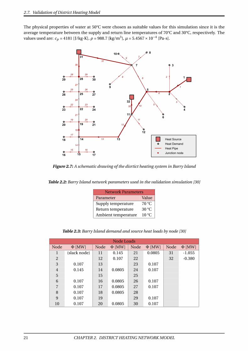
2.7. Validation of District Heating Model
The physical properties of water at 50°C were chosen as suitable values for this simulation since it is theaverage temperature between the supply and return line temperatures of 70°C and 30°C, respectively. Thevalues used are: cp = 4181 [J/kg-K], ρ = 988.7 [kg/m3], µ = 5.4567×10⁻⁴ [Pa-s].
1
2
3
4
5
6
7
8
9
10
11
12
13
14
15 16
18
17
21
19 20
24
22 23
27
25 26
30
28 29
31
32
13
52
1
3
4
6
7
8
9
10
11
12
14
1516 17
18
1920 21
2223 24
2526 27
2829 30
31
32
Heat SourceHeat DemandHeat PipeJunction node
Figure 2.7: A schematic drawing of the disrtict heating system in Barry Island
Table 2.2: Barry Island network parameters used in the validation simulation [30]
Network ParametersParameter ValueSupply temperature 70 °CReturn temperature 30 °CAmbient temperature 10 °C
Table 2.3: Barry Island demand and source heat loads by node [30]
Node LoadsNode Φ [MW] Node Φ [MW] Node Φ [MW] Node Φ [MW]
1 (slack node) 11 0.145 21 0.0805 31 -1.0552 12 0.107 22 32 -0.3803 0.107 13 23 0.1074 0.145 14 0.0805 24 0.1075 15 256 0.107 16 0.0805 26 0.1077 0.107 17 0.0805 27 0.1078 0.107 18 0.0805 289 0.107 19 29 0.107
10 0.107 20 0.0805 30 0.107
21 CHAPTER 2. DISTRICT HEATING NETWORK MODEL

2.7. Validation of District Heating Model
2.7.2 Comparison to Benchmark Simulation
The results of the simulation are very close to the results obtained by Liu in [30], whose results were them-selves validated by a simulation using the commercial software PSS SINCAL (used for planning various typesof distribution networks). The pipe mass flow results of the simulation are all within 1% of the results inLiu’s simulation of the same network, other than pipe 24 which is within 3%. The temperature results are allwithin less than 1% of Liu’s results, with most of the values having error less than 0.01%. (the error here isexpected to be very low, since the difference in temperature is on the order of a few degrees over the entirenetwork, but nonetheless the model shows agreement with the benchmark).
The results are compared to Liu’s results in Tables 2.4 and 2.5 below.
Table 2.4: Mass flow results of the implemented DH model compared to the results byLiu [30]
Mass Flow Rates [kg/s]Pipe DH model Liu Relative error
1 4.799 4.7982 0.017%2 0.651 0.6509 0.015%3 0.876 0.876 0.000%4 3.272 3.2712 0.024%5 0.667 0.6664 0.090%6 -0.876 -0.8802 -0.477%7 0.659 0.6585 0.076%8 0.653 0.6529 0.015%9 0.664 0.6637 0.045%
10 3.481 3.4849 -0.112%11 0.659 0.6593 -0.046%12 4.189 4.1925 -0.083%13 4.189 4.1925 -0.083%14 1.006 1.0062 -0.020%15 0.503 0.5024 0.119%16 0.504 0.5038 0.040%17 0.502 0.5021 -0.020%18 2.187 2.1914 -0.201%19 0.503 0.5031 -0.020%20 0.503 0.503 0.000%21 1.181 1.1852 -0.354%22 0.670 0.6699 0.015%23 0.668 0.6681 -0.015%24 -0.157 -0.1527 2.816%25 0.653 0.6528 0.031%26 0.652 0.6519 0.015%27 -1.462 -1.4574 0.316%28 0.648 0.648 0.000%29 0.649 0.6486 0.062%30 2.759 2.754 0.182%31 3.497 3.5005 -0.100%32 2.247 2.2471 -0.004%
Many of the equations for the model are widely used in all physical models and are therefore the same.However some possible sources of discrepancy between models can be identified:
• The values used for properties of water may differ, especially because values like density, viscosity, andheat capacity are functions of temperature. Variations in these parameters can affect the hydrauliccalculation and also the mass flow required to satisfy thermal loads.
CHAPTER 2. DISTRICT HEATING NETWORK MODEL 22

2.7. Validation of District Heating Model
Table 2.5: Node temperature results of the implemented DH model compared to the re-sults by Liu [30]. The relative errors are based on the excess temperature T ′ (temperatureabove ambient).
Supply Temperatures [°C] Return Temperatures [°C]Node DH model Liu rel error DH model Liu rel error
1 70 70 0.000% 29.631 29.7125 -0.413%2 69.753 69.7533 -0.001% 29.712 29.6314 0.411%3 69.306 69.3054 0.001% 30 30 0.000%4 69.579 69.5787 0.001% 30 30 0.000%5 69.476 69.4764 -0.001% 29.652 29.6517 0.002%6 68.392 68.392 0.000% 30 30 0.000%7 69.656 69.6565 -0.001% 29.688 29.6881 -0.001%8 68.855 68.8555 -0.001% 30 30 0.000%9 69.186 69.1869 -0.002% 30 30 0.000%
10 68.549 68.5491 0.000% 30 30 0.000%11 69.39 69.3902 0.000% 29.726 29.7259 0.001%12 68.809 68.809 0.000% 30 30 0.000%13 69.184 69.1844 -0.001% 29.724 29.7243 -0.002%14 69.056 69.0567 -0.001% 29.767 29.7669 0.001%15 68.928 68.9284 -0.001% 29.774 29.7738 0.001%16 68.312 68.3118 0.000% 30 30 0.000%17 68.211 68.211 0.000% 30 30 0.000%18 68.336 68.3362 0.000% 30 30 0.000%19 68.976 68.9764 -0.001% 29.76 29.7605 -0.003%20 68.257 68.2575 -0.001% 30 30 0.000%21 68.269 68.2693 -0.001% 30 30 0.000%22 68.834 68.8315 0.004% 29.801 29.8015 -0.003%23 68.197 68.1949 0.004% 30 30 0.000%24 68.302 68.2992 0.005% 30 30 0.000%25 69.755 69.7547 0.001% 29.78 29.7795 0.003%26 69.195 69.1947 0.001% 30 30 0.000%27 69.247 69.2461 0.002% 30 30 0.000%28 69.882 69.8821 0.000% 29.796 29.7956 0.002%29 69.486 69.4858 0.000% 30 30 0.000%30 69.445 69.4452 0.000% 30 30 0.000%31 70 70 0.000% 29.655 29.6552 -0.001%32 70 70 0.000% 29.591 29.5906 0.002%
Table 2.6: Heat power calculated for Barry Island source 2 (slack node) [30]
Slack Node PowerΦ [MW]Node DH model Liu rel error
1 0.81004 0.81 0.005%
23 CHAPTER 2. DISTRICT HEATING NETWORK MODEL

2.7. Validation of District Heating Model
• The Darcy friction factor fD is given by an implicit formula, so whether the implicit formula was di-rectly solved or an approximation method was used will affect the friction factor. This will have aneffect on the pipe mass flows in cases of mesh or parallel flows.
In summary, the network and scenario benchmark used for validating the implemented DH model demon-strate functionality for a number of things that are important for a generalizable model to handle.
1. There are multiple demand nodes and multiple source loads. Some models developed in the literatureassume a centralized DH network with a single heat source at the beginning of the line.
2. The network topology is of a meshed configuration and therefore contains loops and multiple trans-port paths. Many DH networks are built or operated in a radial configuration which is inherentlyeasier to model since the node presures are not needed to reach a solution. Consequently, models de-veloped under this assumption cannot accurately find a solution for a meshed network. For the modelto be generalizable it is important to be able to solve meshed topologies, especially since future DHsystems may incorporate many distributed heat sources, making meshed networks more practical.
3. There are multiple nodes that serve only as junctions and do not have an external load attached. Thisis of course not unusual, but if the network were assumed to be a single radial branch then junctionnodes could cause factorization errors when solving the matrix by introducing zero elements.
4. Flow reversal (compared to the assigned flow direction) occurred in three pipes (pipes 6, 24, and 27).Again, a model used for arbitrary network topology must handle reversal of flows since meshes anddistributed producers can easily cause this to happen. Models that assume a radial configuration maynot expect flows to be negative, and may encounter errors in this case.
CHAPTER 2. DISTRICT HEATING NETWORK MODEL 24

Chapter 3
Electricity Network Model
The electric network modeling capability of the software SAInt (Scenario Analysis Interface for Energy Sys-tems) was used in the combined heat-electric simulation. The electrical network steady-state solution wasobtained using SAInt’s built-in AC power flow solver. An overview of the electrical power system was givenin Section 1.2.2, but a brief description of how the electrical power network is modeled in the software isincluded here.
3.1 Power Flow Overview
In the electrical power system nodes are referred to as buses and overhead lines or underground cablesconnect buses together. Transformers step up or down the voltage between different sections of the networkthat they connect. Generators and loads are connected to the network at buses.
The power flow state of an electrical network is fully defined when the voltages and power injections at eachbus and the currents in each branch are known. These are all important to know in order to assure reliabil-ity of the power system. Branch currents must be kept below a certain limit since overcurrents can causeoverheating. The overcurrent limit depends on multiple factors, such as thermal rating of the componentsand environmental factors. Node voltages must be kept within a certain window to assure a consistent andpredictable supply, therefore undervoltages and overvoltages should both be avoided.
The variables of interest in AC power flow are voltage magnitude and angle (|V |, δ) and active and reac-tive power injection (P ,Q) at each bus. The current in each branch is determined when the bus variablesare all known using complex branch admittances. A simple electrical network example is shown in Figure3.1.
~Generator MV / LV
transformer
|V0|,𝞭o
PG,QG I1
P1,Q1 P2,Q2
Bus 1
|V1|,𝞭1 |V2|,𝞭2
I2
|VG|,𝞭G
Demand 1 Demand 2
Bus 1Bus 0Bus G
Line 1 Line 2
Figure 3.1: Simple example of electrical network with one generator and two loads
Active power delivery performs real work, but reactive power is an unavoidable consequence of componentswhich are not purely resistive. Loads which contain motors for example, such as pumps and heat pumps, areinductive loads due to the coils that drive the motors. The lines and cables which make up the network also
25

3.1. Power Flow Overview
are not purely resistive and have a complex impedance due to line impedance and line charging capacitancewhich are considered in AC power flow models. The generic branch model for lines and cables is discussedin section 3.1.4.
3.1.1 Power Flow Equations
The power flow analysis must determine the voltage magnitude |V | and voltage angle δ at each bus. Todetermine these, equations for active and reactive power at each bus, P and Q, respectively, are compiledto create a system of equations. The complex power flow Si [VA] injected into a bus i is given by equation(3.1).
Si =Vi I∗i =Vi
m∑j=1
(V j Yi j
)∗ (3.1)
Where V and I are complex voltages and currents, Yi j is the complex admittance [Ω−1] from bus i to busj , and * denotes the complex conjugate. Taking active power Pi [W] and reactive power Qi [VAr] as thereal and imaginary components of Si , respectively, gives equations (3.2) and (3.3), where δi and δ j are thevoltage angles of bus i and j , and cos(θi j ) is the angle of the complex admittance Yi j between bus i and j .[37]:
Pi (δ, |V |) =n∑
j=1|Vi ||V j ||Yi j |cos
(δi −δ j −θi j
)(3.2)
Qi (δ, |V |) =n∑
j=1|Vi ||V j ||Yi j |si n
(δi −δ j −θi j
)(3.3)
3.1.2 Per-Unit System
To simplify calculations a per-unit system is typically used. A base power Sbase [VA] is defined for the net-work, and a base voltage Vbase [V]) is defined for each voltage region. All other units such as base currentIbase and base impedance Zbase are normalized with respect to these:
Sp.u. = S/Sbase , Vp.u. =V /Vbase , Ip.u. = Sbase /Vbase , Zp.u. =V 2base /Sbase
3.1.3 Ybus Admittance Matrix
The Ybus admittance matrix describes the admittance Y between a bus i and any connected bus j , and isused to determine the branch currents I from the know voltages V at each bus.
I = YbusV (3.4)
For example, a 3-bus network would have a Ybus admittance matrix such as in equation (3.5):
Ybus = Y11 Y12 Y13
Y21 Y22 Y23
Y31 Y32 Y33
,Yi j =− 1
Zi j
Yi i = YiG +∑j ,( j 6=i )
1Zi j
(3.5)
where Yi j is the admittance [Ω−1] and Zi j is the impedance [Ω] between bus i and bus j .
3.1.4 Generic Branch Model (π-model)
SAInt uses a generic branch model (π-circuit) for a single phase line shown in Figure 3.2 [37]. The modelincludes the basic properties of both transmission lines and transformers, including: resistance (R f t ), reac-tance (X f t ), line-charging susceptance (b f t ), voltage angle on the from-side and to-side (δ f and δt ), phase-shift angle (φ f t ), and transformer tap ratio (t f t ).
CHAPTER 3. ELECTRICITY NETWORK MODEL 26

3.2. AC Power Flow Solution
If It
Vt = |Vt|e j𝛿tVf = |Vf|e
j𝛿f
1:tft
Vp Rft jXft
bftj2
bftj2
Figure 3.2: Generic branch model (π-circuit) used in SAInt electrical networks [37] formodeling transmission lines (t f t = 1, φ f t = 0), in-phase transformers (φ f t = 0), andphase-shifting transformers (φ f t 6= 0).
3.2 AC Power Flow Solution
To find a solution to the load flow analysis, the boundary conditions have to be defined for each node. Thetypes of buses are similar to the slack, supply, and demand nodes in the heat network model (see Table 2.1).These are outlined below:
1. Slack Bus (reference bus): |V | and δ are specified, P and Q are computed.
2. PV-Bus (generation bus): P and |V | are specified, δ and Q are computed.
3. PQ-Bus (load bus): P and Q are specified, |V | and δ are computed.
With the boundary conditions defined at each bus, the voltage magnitude and angle |V | and δ, as well asthe active and reactive power P and Q, can be computed at each bus. The branch currents can then bedetermined using the Ybus admittance matrix and equation (3.4).
AC Power Flow Problem
1. All values are converted to per unit [p.u.]2. The Ybus admittance matrix is assembled3. All missing values are assumed at each bus (according to bus type):
|V | = 1.0 p.u., δ = 0°, P = 0 p.u., Q = 0 p.u.4. The linearized system of equations is assembled:
∂∆P∂|V |
∂∆P∂δ
∂∆Q∂|V |
∂∆Q∂δ
[∆|V|∆δ
]=
[∆P∆Q
]Active power mismatch equationsReactive power mismatch equations
(3.6)
(a) Active power equation (3.2) is applied to each node(b) Reactive power equation (3.3) is applied to each node(c) One node is chosen as the reference node, and its equation is replace by defining voltage mag-
nitude and angle.
The AC power flow solution5of the system is found using Newton-Raphson method: the problem is set upas described above and the system of equations is solved to find the next guess; the bus |V |, δ, P , and Qvalues are updated to their new values; and the process is repeated starting at step 4 until the solution con-verges or max iteration count kmax is reached. The branch currents I are finally determined using equation(3.4).
5The AC power flow solver in SAInt is based on the distributed slack bus model [37] and is similar to that developed by Mohapatra[35].
27 CHAPTER 3. ELECTRICITY NETWORK MODEL

Chapter 4
Heat-Electric Combined Model
Chapter 2 presented the method for implementing a heat network load flow model and Chapter 3 describedhow the AC power flow simulation works in the SAInt software. This chapter details how the heat and electricnetworks are linked through coupling components using the energy hub concept to embody their opera-tion. First the coupling components are defined mathematically, then the energy hub concept is appliedto this context, and finally the algorithm for running a combined heat-electric network simulation is illus-trated.
4.1 Network Coupling Components
The interactions between the heat and electrical networks occur in large part by the components whichare connected to both systems. The coupling components considered here include heat pumps, electricresistor heaters, combined heat and power plants, and circulation pumps.
4.1.1 Heat Pumps
Heat pumps use electricity to produce heat and/or cooling. From a thermodynamic perspective a heatpump transports heat from a cold side to a hot side, using mechanical work Wi n to drive a compressor inthe thermodynamic cycle as represented in equation (4.1) where Φout is the useful heat output to the hotside, in the case of a HP used for heating. Φout corresponds to Φq in the heat power equation 2.7 in the DHnetwork.
COP = Φout
Wi n(4.1)
In practice the mechanical work supplied to the compressor is provided by an electrically-driven motor, sothe COP is typically given in terms of the electrical power input PHP and heat output ΦHP , as in equation(4.2). According to a recent survey [13], the COP of air-source HPs ranges from about 3.2 - 4.5, and fromabout 4.2 - 5.2 for ground-source HPs. The COP depends on the hot and cold side temperatures, and maydecrease with increased load.
COP = ΦHP
PHP(4.2)
Since heat pumps contain motors and power electronics they may have an associated power factor that isnot equal to 1. A survey of heat pumps and their measured power factors in [25] found their displacementpower factors to be in the range of 0.88 lagging to 0.97 leading. Lagging power factors are a result of theinductive load of the motor which drives the compressor. In the case of leading power factors, it is often dueto a capacitive DC filter included in an input rectifier in modern equipment.
28

4.1. Network Coupling Components
4.1.2 Electric Boilers
An electric resistor heater (ERH) or electric boiler (EB) uses electricity to produce heat by running currentthrough a resistor. The resistor heats up, and this heat is given to a heat transfer fluid such as water.
Electric boilers can reach higher temperatures than heat pumps, and they are also far simpler and less ex-pensive. However EBs do not have the advantage of a COP greater than 1, so they are less efficient comparedto a HP. That said, the resistor converts nearly all of the electrical power into heat, and the efficiency is veryclose to 100%, with 99% being a typical estimate.
ηEB = ΦEB
PEB≈ 99% (4.3)
Electric heaters of this kind, when incorporated into a DH network, are best suited as peak-load units sincethey are less efficient but also cheap and reliable. Since they are purely resistive loads there is also no con-sumption of reactive power.
4.1.3 Combined Heat and Power Plants
Combined Heat and Power (CHP) plants produce heat and electricity and can come in many different forms.They may burn fuel to run a Rankine or Brayton cycle, use heat collected by a concentrated solar powerplant, or could even use the waste heat produced by a fuel cell power plant. The three most common typesof CHP units are gas turbines, internal combustion engines, and steam turbine extraction condensing units[55] which are discussed in the following sections. Examples of the operating ranges of the different CHPplant types are shown in Figure 4.1.
Pcon
PCHP
𝚽CHP
PCHP
𝚽CHP
A(𝚽1,P1)
B(𝚽2,P2)
C(𝚽3,P3)
D(𝚽4,P4)
Ele
ctric
al p
ower
[W]
Useful heat power [W] Useful heat power [W]
Ele
ctric
al p
ower
[W]
-1/Z
Δ𝚽ΔP
Δ𝚽
ΔPcm
Figure 4.1: CHP operating ranges: (left) gas turbines or internal combustion units,(right) steam turbine extraction condensing units.
Gas turbines & internal combustion (reciprocating) units
Gas turbines and internal combustion engines can be described with a simple linear relationship betweenheat and power production, as in equation (4.4).
ΦC HP = cm ·PC HP (4.4)
whhere cm is the heat-to-power ratio. The heat output is set with respect to electrical power output, leavingno real flexibility. The unit can be driven by heat demand or electricity demand, but the production of theother energy vector must follow this.
29 CHAPTER 4. HEAT-ELECTRIC COMBINED MODEL

4.2. Energy Hubs
Steam turbine extraction-condensing units
Steam turbine units with extraction-condensing capability have more flexibility with their heat-to-powerproduction.
In an extraction steam turbine, vapor can be extracted from a turbine before being fully expanded in or-der to extract its heat. With multistage turbines there is the opportunity to extract steam from multiplestages. The feasible operating region of an extraction-condensing steam turbine is a polyhedron definedby multiple extreme points (Φm ,P m),m = 1,2, ... [55, 61], exemplified in Figure 4.1, depending on the plantconfiguration.
P =∑kαk P k , Φ=∑
kαkΦk
0 ≤αk ≤ 1, ∀k,∑
k αk = 1
(4.5)
The electrical power and heat production can be determined with a convex combination of the extremepoints, as in equation (4.5) [55]
The path between points C and D in Figure 4.1 was chosen to represent the operation curve of the extraction-condensing steam turbine (ECST) in this thesis. Point D represents the unit operating in full condensingmode, producing power Pcon . As the operating point moves along the path to point C the unit extracts moresteam in order to provide useful heat, and in turn generates less electrical power. The equations governingthe operation in this region are as follows [30]:
Z = ∆Φ∆P
= ΦC HP
Pcon −PC HP(4.6)
PC HP = Pcon − ΦC HP
Z(4.7)
4.1.4 Circulation Pumps
Electrically-driven circulation pumps are required to provide the pressure to the DH supply network andovercome the head losses associated from the water circulation. Although the pumps do not contribute tothe thermal load of the DH network, their electrical power draw is based on the state of the DH network andtherefore act as another component which interacts with both networks.
The pump power Pp [W] required to provide increase the hydraulic head hp [m] of a mass flowing throughthe pump mp [kg/s] is given by equation (4.8).
Ppηp = mp g hp (4.8)
where ηp is the electrical efficiency of the pump [-], and g is the acceleration of gravity (9.81 [m/s2]).
4.2 Energy Hubs
The implementation of the coupling components to link the networks in the combined heat-electric modelis based on the energy hub concept, which was described in Section 1.3.2. In terms of information flowan energy hub acts as a mediator between the heat externals and the electric externals. When values fromone network are updated, the hub performs the calculations to determine how the other network externalshould be set. In this way the state of one network can be reflected in the state of the other network.
For example, as shown in Figure 4.2 when the heat power output ΦHP of a heat pump is set, the hub calcu-lates the active and reactive power inputs PHP and QHP needed to run the HP cycle and the pump. It then
CHAPTER 4. HEAT-ELECTRIC COMBINED MODEL 30

4.3. Heat Electric Combined Solver
sets the electric external accordingly. In this way the state of the heat network is reflected in the state of theelectricity network. Electric boilers and CHP plants are modeled in a similar fashion.
HP cyclePHP
QHP
𝚽HP
hHP
physical flows
pump
HP cycle𝚽HP
hHP
PHP
QHP
information flows
pump
power factor
𝚽amb
Figure 4.2: Energy hub implementation of a heat pump
Two additional notes about the energy hubs implementation:
• The energy hubs include the circulation pumps inside. Thus, instead of creating pumps as a separatecoupling component they are embedded as a parasitic electricity consumption in each of the heatsources.
• The power factor p. f . is used to define the active and reactive power loads of the electric demands,and is the ratio of real power to apparent power. The reactive power consumption Q for the HP andits circulation pump is determined from P and the power factor.
4.3 Heat Electric Combined Solver
The combined simulation of heat and electrical networks is achieved by way of three main components:
• Heat Solver (developed in this thesis, and described in Chapter 2)
• Electric Solver (the commercial software SAInt was used for AC power flow, described in Chapter 3)
• Coupling Components (described in this Chapter, and modeled as energy hubs)
The process the heat electric combined solver uses to arrive at the heat network load flow solution is il-lustrated in Figure 4.3. The combined solver iteratively switches between the Heat Solver and the ElectricSolver. When a solution in one solver has been found, the setpoints for each coupling component are up-dated to reflect the solution before switching to the other solver.
For example, the Heat Solver converges and a new value of ΦHP is found for a heat pump. The heat pump’selectrical power PHP is then calculated by using Equation (4.2) for the thermodynamic cycle and Equation(4.8) for the circulation pump, and finally the reactive power is calculated based on the power factor. Thiselectrical power result is updated in the electrical network. The rest of the coupling components are updatedaccordingly and the Electric Solver begins.
Each combined iteration cycle kc the solver checks the residual between the current and previous load flowsolution for both the Heat and Electric networks,∆H Net and∆E Net , respectively. A solution has convergedif both network residuals are below their prescribed thresholds εh and εe . 6
6The heat and electrical network values are computed using base values on different orders of magnitude (W for heat, and MWfor electric), so it is necessary for the values of εh and εe to reflect this.
31 CHAPTER 4. HEAT-ELECTRIC COMBINED MODEL

4.3. Heat Electric Combined Solver
Electric Solver
Heat SolverEnergy Hubs
Set Heat network initial state
Solve state of Heat network.Update Heat network values:
ṁ, H, Ts , Tr
Start
Enddid not
converge
EndSolution
converged
Solve state of Electric network.Update Electric network values:
|V|, 𝛅, P, Q
no
yes
yes
no
Heat network setpoints
ɸq, Href, Ts , Tr
Electric network setpoints
P, Q, |Vref|, 𝛅ref
Calculate ɸq
Calculate P, Q
ɸhub
(P, Q)hub
Set Electric network initial state
kc = 0
ɸhub
Max(ΔHNet) ≤ 𝜺hand
Max(ΔENet) ≤ 𝜺e ?
Calculate ΔHNet(difference between current and
previous HNet solution ɸq values)
Calculate ΔENet(difference between current and previous ENet solution P values)
Phub
Initialize Heat and Electric networks
kc = kc+1
kc ≤ kc,max ?
Figure 4.3: Heat Electric Combined Solver Flowchart
CHAPTER 4. HEAT-ELECTRIC COMBINED MODEL 32

Chapter 5
Case Study
A case study was undertaken in order to understand the behavior of the combined Heat-Electric solver, andto see how the combined solution differed from those obtained by simulating the networks individually.Simple heat and electrical distribution networks were created for the case study. Each network was solvedindividually with the standalone heat or electric load flow simulations, respectively. The two case networkswere then coupled by energy hubs and input into combined Heat-Electric network solver. The effect of slackparticipation is also investigated by running the case study in two different scenarios of slack participationin the heat network.
This chapter describes the goals of the case study and the networks used. The approach for setting the initialconditions is outlined, and then the subsequent simulation results are given.
5.1 Strategy of the Investigation
The goal of the case study was primarily to understand how a load flow solution obtained from the com-bined Heat-Electric solver can differ from those obtained by simulating the networks individually. Differentpossible approaches for the investigation were considered, but complexity and real-world accuracy had tobe balanced against feasibility and simplicity.
The results can be complex to analyze, so an effort was made to design the networks as simply as possi-ble while still maintaining a structure that is representative of real-world heat and electricity distributionnetworks. Both networks were designed as branched networks with radial operation.
A 2-way interaction between the heat and electricity networks was necessary for significant effects of thecombined simulation to be present, so two CHP plants were chosen to provide the electrical power, and aheat pump station was included for additional heat production.
5.2 Network Descriptions
5.2.1 Heat Network
The district heating network created for the case study is shown in Figure 5.1. It has 20 demand nodes,each consuming 20 kW of heat. There are 3 heat supply nodes: One CHP extraction-condensing steamturbine (ECST), one CHP gas turbine (GT), and one heat pump station (HP). The CHP (ECST) at node A isthe primary heat slack source, and therefore node A serves as the reference node for pressure head. Theheat network parameters are given in Appendix D.
33

5.2. Network Descriptions
CHP (ECST)
CHP (GT)
HP
A
B
C
0 1 2 3 45
1c
1d
1b
1a
2c
2d
2b
2a
3c
3d
3b
3a
4c
4d
4b
4a
5c
5d
5b
5a
A
C
B 0 1 2 3 4
1a
1b
1c
1d
2a
2b
2c
2d
3a
3b
3c
3d
4a
4b
4c
4d
5a
5b
5c
5d
Figure 5.1: Heat network model used for the case study
5.2.2 Electric Network
The electrical network model created for the case study is shown in Figure 5.2. In the LV (0.4 kV) networkthere are 20 demand nodes, each with a load of 3 kW at a power factor of p.f. = 1.0. In the MV (10 kV) sidethere are 2 generators and one demand. The CHP plants are the generators, and the HP is the demand in theMV side. The CHP (GT) at bus C is the electrical slack generator, and therefore bus C serves as the referencenode for voltage angle. The electric network parameters are given in Appendix D.
~
~
CHP (ECST)
CHP (GT)
HP
10kV / 0.4kV1b 2b 3b 4b 5b 5a 5c 5d 4d 3d 2d 1d
4a 3a 2a 1a
4c 3c 2c 1c0
00
A
B
C
A
B
C
1 2 3 4 5 6 7 8 9 10 11 12
1314 15 16
1718 19 20
Figure 5.2: Electric network model used for the case study
5.2.3 Combined Heat-Electric Network
The combined Heat-Electric network model couples the two networks together via 3 coupling points: TwoCHP plants supply power to both networks, and a heat pump station uses electricity to produce heat forthe DH network. Since these three units all must pump water into the heat network’s supply line, each one
CHAPTER 5. CASE STUDY 34

5.2. Network Descriptions
includes an electrically-driven circulation pump. 7
Table 5.1: Heat-Electric network coupling points
Coupling Component Heat Net Electric Net Coupling Parameters
CHP (ECST) (node A) supply (bus A) generator Z = 8.0, Pcon = 60 kW
HP (node B) supply (bus B) demand COP = 4.0, p.f. = 0.9
CHP (GT) (node C) supply (bus C) generator cm = 1.3
Circulation Pumps 7 (nodes A,B,C) (buses A,B,C) η = 0.7, p.f. = 0.9
CHP (ECST)
CHP (GT)
HP
~
~
10 kV
0.4 kV
1c
1d
1b
1a
2c
2d
2b
2a
3c
3d
3b
3a
4c
4d
4b
4a
5c
5d
5b
5a
A
B
C
0 1 2 3 45
A
C
B
00
0
Figure 5.3: Combined Heat-Electric network model used for the case study
5.2.4 Slack Participation
Combined heat and power plants often operate primarily driven by the demand of one energy vector andsell the other which is produced as a byproduct. In this case study the ECST was chosen to be heat demanddriven, and the GT was chosen to be electricity demand driven. The HP was also chosen to participate inheat slack since its sole purpose is to provide heat to the DH network. The participation in heat slack wasdistributed among the HP and ECST as given in Table 5.2. The values of βEC ST and βHP were chosen tobe proportional to the initial power setpoints ΦSP . In other words, since the HP has a smaller output itsparticipation should reflect this. The the GT is the participating generator in the electricity network.
Table 5.2: Distributed slack participation among power producers
Heat participation Electric participationβEC ST βHP βGT βEC ST βGT
0.85 0.15 1.0
5.2.5 Initial Setpoints
In order for the solver to converge to a solution, the initial setpoints of the generators and heat suppliesneeded to be specified relatively close to the actual solution. The process for determining a suitable startingpoint is outlined below:
7The electrical demand of each pump is not modeled as a separate electrical load, but instead is considered a parasitic con-sumption of electricity by each unit.
35 CHAPTER 5. CASE STUDY

5.3. Results
1. Specify the HP heat outputΦHP , and determine electrical draw PHP using coupling equation (4.2).
2. Assume zero losses:
• No temperature drop or head loss in pipes; no pumping power is required
• No resistive losses or reactive power component in electrical lines; only real power is involved
3. Given 2 CHP plants (each with heat and electric outputs), 2 network demands, and 2 coupling equa-tions (4.4) and (4.7): there are 4 unknowns and 4 equations. Solve forΦEC ST , PEC ST ,ΦGT , PGT .
The initial conditions obtained from this process were used in all of the simulations in order to assure aclearer comparison between the separate and combined network solutions. The initial power setpoints forall three coupling components are:
Table 5.3: Coupling components initial power setpoints
ECST HP GT
ΦSPEC ST = 287,097 W ΦSP
HP = 50,000 W ΦSPGT = 62,903 W
P SPEC ST = 24,113 W P SP
HP = 12,500 W P SPGT = 48,387 W
5.3 Results
5.3.1 Combined Heat-Electric Solution
The combined heat-electric simulation (CHEsim) converged to a solution in 7 iterations. A tolerance of 1W was used for both εh and εe . Figure 5.4 shows the power values of each coupling component during theiteration process. The full load flow results are given in Appendix E.
Figure 5.4: Iterative convergence of the Heat-Electric combined solver, which reached asolution after 7 iterations. The charts show the heat and electric power of each couplingcomponent.
5.3.2 Combined Solution Compared to Individual Solutions
The networks were simulated again on individual heat and electric network solvers (Hsim and Esim, respec-tively) using the same starting conditions. The results for coupling component loads of all the simulationsare reported in Table 5.4. Missing values from standalone heat and electric individual results were restored
CHAPTER 5. CASE STUDY 36
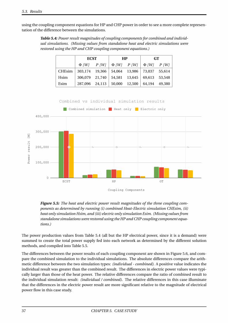
5.3. Results
using the coupling component equations for HP and CHP power in order to see a more complete represen-tation of the difference between the simulations.
Table 5.4: Power result magnitudes of coupling components for combined and individ-ual simulations. (Missing values from standalone heat and electric simulations wererestored using the HP and CHP coupling component equations.)
ECST HP GT
Φ [W] P [W] Φ [W] P [W] Φ [W] P [W]
CHEsim 303,174 19,366 54,064 13,986 73,037 55,614
Hsim 306,079 21,740 54,581 13,645 69,613 53,548
Esim 287,096 24,113 50,000 12,500 64,194 49,380
Φ P Φ P Φ PCoupling Components
Power result [W]
0
100,000
200,000
300,000
400,000
ECST HP GT
Combined simulation Heat only Electric only
Combined vs individual simulation results
Figure 5.5: The heat and electric power result magnitudes of the three coupling com-ponents as determined by running (i) combined Heat-Electric simulation CHEsim, (ii)heat only simulation Hsim, and (iii) electric only simulation Esim. (Missing values fromstandalone simulations were restored using the HP and CHP coupling component equa-tions.)
The power production values from Table 5.4 (all but the HP electrical power, since it is a demand) weresummed to create the total power supply fed into each network as determined by the different solutionmethods, and compiled into Table 5.5.
The differences between the power results of each coupling component are shown in Figure 5.6, and com-pare the combined simulation to the individual simulations. The absolute differences compare the arith-metic difference between the two simulation types: (individual - combined). A positive value indicates theindividual result was greater than the combined result. The differences in electric power values were typi-cally larger than those of the heat power. The relative differences compare the ratio of combined result tothe individual simulation result: (individual / combined). The relative differences in this case illuminatethat the differences in the electric power result are more significant relative to the magnitude of electricalpower flow in this case study.
37 CHAPTER 5. CASE STUDY

5.3. Results
Table 5.5: Total network supply power for combined and individual simulations
Total Network Supply Power
Φ [W] P [W]
CHEsim 430,275 74,981
Hsim 430,273 75,289
Esim 401,290 73,493
Figure 5.6: Absolute and relative differences between the results of the combined sim-ulation and the individual heat and electric simulations, respectively. A positive dif-ference indicates that the result in the individual simulation was greater in magnitudethan that of the combined simulation.
5.3.3 Network-Level Results
The main total power results of each network as a whole are contained in Table 5.6. The network efficiencyonly considers the losses from the transport of energy through the network, and does not consider the pri-mary energy input.
Table 5.6: Network-level load flow results
Heat Network
Demand [W] Supply [W] Φloss [W] Pump power [W] Heat Network Efficiency 8
CHEsim 400,000 430,275 30,275 2642 92.4%Hsim 400,000 430,273 30,273 2640 92.4%
Electricity Network
Demand [W] Supply [W] Ploss [W] Electric Network Efficiency
CHEsim 73,986 74,981 994 98.7%Esim 72,500 73,493 993 98.6%
The power values shown in Figure 5.6 were aggregated to show how the combined simulation results com-pared to the individual simulation results on a network level. Figure 5.7 shows these aggregated values. Φdiff and P diff sum together the differences in heat and electric power shown in Figure 5.6. The differencesin power in this case show that positive and negative differences between load among the coupling compo-nents in the simulations approximately balance each other, since the aggregate sums are close to zero. Thelast three bars aggregate the magnitudes of the differences only, ignoring the canceling out of positive andnegative values. The aggregated values represent how much power is reallocated throughout the network.
8Heat network efficiency includes both thermal and hydraulic losses.
CHAPTER 5. CASE STUDY 38

5.3. Results
In other words, even though the total power production and consumption are approximately equal in thedifferent simulations, the allocation of where each unit of power is produced is different in the combinedsimulation than in the individual heat or electric simulations.
Net power difference [W]
-5,000
0
5,000
10,000
15,000
20,000
Φ diff P diff |Φ diff| |P diff| |Φ+P diff|
Total network differences
Figure 5.7: Total network differences between the combined simulation result and theindividual simulation results. The first two bars represent the sums of the differencesof all heat and electric power results of the coupling components.* The last three barsrepresent the sums of the magnitudes of the differences only.
*(Φ diff is too small to show in the graph but is equal to -2 W.)
The power reallocation is shown again in Figure 5.8, alongside the same data renormalized relative to thenetwork demands. The amount of electric power that is reallocated in the combined simulation is greaterthan the amount of heat power reallocated. The renormalized (relative) reallocation is again greater for theelectrical network than the heat network, but the difference is more pronounced. The total heat demand isapproximately 5.5 times greater than the electrical demand. The electric reallocation is approximately 1.8times greater than the heat reallocation. Putting these together, the relative electric reallocation is approxi-mately 10 times greater than the relative heat reallocation.
Figure 5.8: Absolute and relative differences between the total network allocation ofheat and electrical power in the results of the combined simulation compared to theindividual simulations.
39 CHAPTER 5. CASE STUDY

5.4. Discussion
5.4 Discussion
The results of the combined simulation offer several insights when compared to the standalone heat andelectric simulations.
One of the first things to notice is when looking at the iteration convergence in Figure 5.4 there is an increasein electric power consumption of the HP before the heat production increases. This is explained by theparasitic electrical load of the pump. Even though the electrical power used for running the heat pumpthermodynamic cycle is not affected, the circulation pump requires electrical power which depends on thehydraulic head it needs to supply. This head increase depends on the hydraulic state of the DH networkload flow which the Esim does not take into account.
The HP heat power output was altered from the setpoint because of its share of distributed slack partic-ipation. When looking at the absolute difference comparison in Figure 5.6 the Hsim simulation showedhigher HP heat output than the CHEsim, while the Esim showed lower HP electrical consumption than theCHEsim. The Esim did not take into account the HP slack participation, so it underestimated the electricpower required to increase its heat output. The Hsim result of HP heat output was closer, and the differencecompared to the CHEsim was due to the fact that the Hsim did not adjust the power output of the GT, whichwould have provided more heat.
In the Hsim the heat network losses were made up for by increasing the output of ECST and HP. In the Esimthe electric network losses were made up for by increasing the output of the GT. The HNET heat losses wereapproximately 30 times greater than the ENET losses (see Table 5.6), so the influence of losses in the HNETwas a much greater driver in the combined simulation which the Esim could not adequately capture.
Regardless of the relative network losses, the changes in the coupling components’ operational states allaffect each other. When the output of one unit increases, other producers must decrease their output inorder to bring back a balance of supply and demand. This reallocation of power consequently changesthe network load flow state, which affects the network losses. These inter-dependencies simply cannot beaccounted for in the individual simulations. A combined simulation is necessary to correctly coordinate allof the units.
Tables 5.5 and 5.6 show clearly that the Esim fell short in estimating the total network heat supply by anamount that is comparable to the heat network losses (around 30 kW). The Esim also underestimated theelectric power needs, although by very little. The Esim was only able to account for the losses in the electricnetwork, and so it fell short of the true needs of the combined network and was not able to take into accountheat losses or pumping power required by the DH network. It is tempting to assume that the degree thateach individual simulation falls short for total network supply should be around the degree of losses in theother network, but this does not seem to be exactly true if we look at how the Hsim compared to the CHEsim.The Hsim predicted very close to the heat power needs compared to the CHEsim. However the inferredvalues from the Hsim slightly overestimated the electrical power supply. It is not clear what the cause ofthis is. It’s notable that the difference is roughly comparable to the level of losses in the electrical network,though it is not likely that this is the cause of the difference. A potential explanation is that the differenceis simply due to the difference in heat allocation which causes unchecked reallocations in electrical powerbecause of the CHP plants’ operation curves.9
The individual simulations do, however, closely match the total network supply of their own network whencompared to the CHEsim. The Hsim and CHEsim total heat supply are essentially identical, and the Esimand CHEsim total electric supply are within 2% of the electric demand. This indicates that the individualsimulations were accurate when compared to the combined simulation and that any differences are likelydue to a difference in network losses.10But again, even though the individual simulations were close fortheir own network they failed to accurately match the needs of the other network, and overall deviated in
9If this is the case then the effect is hidden by the fact that the two CHP operation characteristics work against each other (anincrease in ECST Φ decreases P , but an increase in GT Φ increases P .) So if two GTs were used as the CHP plants then the Hsimestimate of electric power would be much farther off.
CHAPTER 5. CASE STUDY 40

5.5. Limitations of the Study
their estimations.
Looking beyond the total net power supply reveals more meaningful differences between the combinedsimulation and the individual simulations. Figures 5.7 and 5.8 demonstrate the extent of reallocation clearly.Again, as was stated in the previous paragraph the individual simulations were relatively accurate to theneeds of their own network in terms of total network supply. In other words the total amount of powerproduced was comparable to what the combined network truly needed. The differences beyond that arefound in how the distribution of power is allocated among the network externals.
Figure 5.8 shows that there are positive and negative differences between how power is allocated amongthe units but they mostly cancel each other out for both networks. Figure 5.7 aggregates the magnitudesof these differences to show that the locations where power is produced is meaningfully different in thecombined simulation when compared to the individual simulations. Figure 5.6 compares the HNET andENET reallocation and illustrates two interesting points: First is that the electrical power reallocation isgreater than the heat power reallocation. Since the HNET demand is much higher than the ENET demand(by a factor of about 5.5) it suggests that the HNET is had more influence on the ENET solution in thecombined simulation. Secondly when these power reallocations are normalized with respect to the HNETand ENET demands the ENET relative reallocation is much larger than that of the HNET (by a factor of about10). This suggests that not only did the HNET influence the ENET soution, it had a disproportionately largerinfluence.
Differences in power allocation could affect some important results of load flow analysis. One of the rea-sons for using load flow simulation is to determine whether some situations result in parts of the networkexperiencing adverse conditions. Overcurrent in lines and over/under-voltage in buses, for example, arekey indicators which are considered when designing electrical networks. These key indicators could be af-fected if the true operational point is significantly reallocated. For example: an electric network load flowsimulation might show that all line currents and bus voltages are at acceptable levels, but if it is coupledwith a heat network it is possible that the combined heat-electric solution would indicate that, because ofa difference in power allocation, there is congestion in a line experiencing an overcurrent. In this regarda combined network solution is important to gain a more complete understanding of the load flow thatindividual network simulations are unable to produce.
5.5 Limitations of the Study
The study presented in this thesis was not all-encompassing and had some limitations, which are outlinehere.
• Constraint violations, such as overloading of lines or pipes or voltages outside of the proper rangewere not looked at or considered. The load flow simply calculated the state of the network and wasnot able to adjust for such violations.
• The network in the case study was relatively small and was a simple radial configuration and load dis-tribution was uniform which left less opportunity for major differences in load flow. A larger and morecomplex network would have larger losses, and the effect of reallocation of power could subsequentlyhave a much larger effect on these losses, expecially in a meshed network.
• The case study network was an islanded grid with no connection to the external power grid. Althoughthis is possible, it would be more applicable to consider a system that is not isolated from the largerpower system.
• There were some parameters which were treated as constant that in reality can change with condi-tions. For example heat capacity of water changes with temperature, but the value used in this modelwas constant. Elevation was assumed constant, but real elevation changes could have drastic effect
10The case study network is radial with all sources meeting at a junction before continuing to the demand area, so the losses willnot vary all that much. In a larger network, especially one with a more complex configuration (for example a meshed topology)where the load flow has more freedom and the losses can change more, this difference might also be larger.
41 CHAPTER 5. CASE STUDY

5.5. Limitations of the Study
on the pump power required in the DH network. Other operational parameters were assumed con-stant, such as the heat pump COP and the heat to power ratio for the CHP plant.
• Although an effort was made to design the case study network using realistic values, some values werechosen for convenience. For example, all of the heat demands were equal, which is not realistic. Thesesimplifications were justified by the qualitative nature of the study: the aim was to investigate trendsand compare simulations, not to determine exact numbers.
• Finally the conclusions drawn from the case study in this thesis cannot represent all possible scenar-ios, so the findings presented here can only be assumed to apply to the network studied.
CHAPTER 5. CASE STUDY 42

Chapter 6
Conclusion
The main research question investigated in this thesis was to determine what benefits there are by run-ning a combined heat-electric network simulation compared to simulating the networks separately, if thenetworks are linked by coupling components such as CHP plants or heat pumps. In order to answer thisquestion the following steps were taken:
1. A physics-based district heating network model was implemented for performing steady-state loadflow analysis including distributed slack participation.
2. The method for performing load flow analysis of electrical networks was briefly described in orderto inform about the underlying functionality of the commercial solver used for the electrical networksimulation.
3. The coupling components which link the heat and electric networks together were defined, and theequations which govern their power flows linking the heat and electricity networks were given. Thesewere encapsulated as energy hubs which mediated data exchange between solvers and performed thecoupling calculations.
4. A combined Heat-Electric network solver was implemented which iteratively solved the two networksusing energy hubs to facilitate the coupling between them.
5. Finally, a case study was performed in which a coupled heat and electric network was subject to loadflow simulations by the combined heat-electric solver, the heat network solver, and the electric net-work solver. The resulting simulation results were compared and conclusions were drawn on whatdifferences there were and what caused these differences in this specific case.
The case study performed revealed a few main areas of difference between the combined simulation andthe individual simulations:
Network losses drive the actual operating point (solution) away from the initial guess. A standalone simula-tion of a single network will neglect the losses of the other network because it does not have access to thatinformation. Although these losses could be assumed and added back into a single network simulation,that alone does not take into account the necessary changes in the allocation of power dispatch and maynot improve the accuracy of the estimation.
Reallocation of the power dispatch among the coupling components turned out to be significant, but thenet effect of this power reallocation was concealed if only the total network supply power was looked at,since the positive and negative differences mostly balanced each other out. However when the magnitudesof differences in power allocation were compared it was clear that the combined network solution had asignificantly different allocation of power dispatch among the coupling components. The larger influence ofthe heat network in the case study caused the electric network to experience a more significant reallocationrelative to the total electric load.
Although the reallocation did not affect the total supply-demand balance as significantly, it could affect
43

some important results of load flow analysis. Key indicators from load flow analysis which are used in net-work planning like current congestion, over-voltage, under-voltage, underpressure, and losses could all beaffected if the true operational point is significantly reallocated. In this regard a combined network solutionis important to gain a more complete understanding of the load flow that individual network simulationsare unable to produce.
Finally, since the network studied in the case study was relatively small and simple it is likely that larger andmore complex networks - especially ones with meshed topologies, distributed generation, a more variedassortment of loads, and higher losses - may display more pronounced differences between isolated andcombined load flow simulations.
Contributions of the Thesis
The contributions of the thesis are as follows:
• A general physics-based model for performing steady-state load flow simulation on district heatingnetworks of arbitrary topology was created and described.
• A simple implementation for distributed slack participation was given and implemented in the dis-trict heating network model.
• A method for performing a combined heat-electric network load flow simulation using a heat net-work solver and an electric network solver was provided, using an energy hub object as a mediator tofacilitate coupling between the networks.
• A case study was performed which illuminated certain benefits of performing a coupled heat-electricnetwork simulation compared to simulating the networks separately.
Recommendations for Future Work
Some recommendations for future work are as follows:
• A longitudinal study of many case networks with a range of sizes and degrees of coupling would pro-vide more insight into general benefits of coupled network simulation.
• Further investigation into the impacts of distributed slack and distributed generation on the com-bined network load flow results could be of interest.
• District heating and cooling networks should be similarly studied coupled with electrical networks.
• Additional networks could be included to investigate what the benefits of coupled simulation are. Forexample: heat-electric-gas network simulation.
• Similar investigations with optimal power flow simulations could provide key insights into how theoptimization differs when run in a combined simulation compared to individual network simulations.
• The model should be further developed to include a transient heat network model, so that additionaldynamic simulation studies can be performed. This could be exceptionally rich in possibility for studyas it could include thermal energy storage, thermal inertia of the DH network, production rampingrates, demand side management, and other ways in which the heat network could add flexibility tothe electrical network.
The topic of combined simulation of heat and electricity networks is an important part of the sustainableenergy transition. The need to decarbonize the heat sector means that heat will be further electrified, sothe interaction between heat and electricity networks is becoming more important. Interconnected energysystems are increasingly interesting from the standpoints of efficiency, flexibility, and security of supply,and load flow analysis is one of the first tools used in making network planning decisions. Understandinghow the systems work together is critical, and understanding the limitations of how they are modeled andsimulated can have a decisive influence.
CHAPTER 6. CONCLUSION 44

Bibliography
[1] M. Abeysekera and J. Wu. Method for simultaneous power flow analysis in coupled multi-vector energynetworks, 2015.
[2] M. Akmal, B. Fox, J. D. Morrow, and T. Littler. Impact of heat pump load on distribution networks. IETGeneration, Transmission & Distribution, 8(12):2065–2073, 2014.
[3] B. Aluisio, M. Dicorato, G. Forte, G. Litrico, and M. Trovato. Integration of heat production and thermalcomfort models in microgrid operation planning, 2018.
[4] I. d. H. Arce, I. del Hoyo Arce, S. H. López, S. L. Perez, M. Rämä, K. Klobut, and J. A. Febres. Models forfast modelling of district heating and cooling networks, 2018.
[5] L. Bin. Probabilistic power flow model to study uncertainty in power system network based upon pointestimation method, 2017.
[6] A. Bloess, W.-P. Schill, and A. Zerrahn. Power-to-heat for renewable energy integration: A review oftechnologies, modeling approaches, and flexibility potentials, 2018.
[7] I. C. Change et al. Mitigation of climate change. Contribution of Working Group III to the Fifth Assess-ment Report of the Intergovernmental Panel on Climate Change, 1454, 2014.
[8] D. Chen, X. Hu, Y. Li, R. Wang, Z. Abbas, S. Zeng, and L. Wang. Nodal-pressure-based heating flowmodel for analyzing heating networks in integrated energy systems, 2020.
[9] D. Clamond. Efficient resolution of the colebrook equation. Industrial & Engineering Chemistry Re-search, 48(7):3665–3671, 2009.
[10] D. Connolly, H. Lund, B. V. Mathiesen, S. Werner, B. Möller, U. Persson, T. Boermans, D. Trier, P. A.Østergaard, and S. Nielsen. Heat roadmap europe: Combining district heating with heat savings todecarbonise the eu energy system. Energy policy, 65:475–489, 2014.
[11] J. Danielewicz, B. Sniechowska, M. A. Sayegh, N. Fidorów, and H. Jouhara. Three-dimensional nu-merical model of heat losses from district heating network pre-insulated pipes buried in the ground,2016.
[12] J. Duquette, A. Rowe, and P. Wild. Thermal performance of a steady state physical pipe model forsimulating district heating grids with variable flow, 2016.
[13] D. Fischer and H. Madani. On heat pumps in smart grids: A review. Renewable and Sustainable EnergyReviews, 70:342–357, 2017.
[14] X. Gao, G. Li, X. Zhang, D. Shi, X. Wang, and Z. Bie. An iteration method for optimal energy flow ofcombined heating and electricity system, 2019.
[15] M. Geidl and G. Andersson. Optimal power dispatch and conversion in systems with multiple energycarriers. In Proc. 15th Power Systems Computation Conference (PSCC), 2005.
[16] M. Geidl and G. Andersson. Optimal power flow of multiple energy carriers. IEEE Transactions onpower systems, 22(1):145–155, 2007.
I

Bibliography
[17] L. Giraud, R. Bavière, C. Paulus, M. Vallée, and J.-F. Robin. Dynamic modelling, experimental validationand simulation of a virtual district heating network. In ECOS 2015 - The 28th International Conferenceon Efficiency, Cost, Optimization, Simulation and Environmental Impact of Energy Systems, 2015.
[18] S. Grosswindhager, M. Kozek, A. Voigt, and L. Haffner. Fuzzy predictive control of district heatingnetwork, 2013.
[19] S. Grosswindhager, A. Voigt, and M. Kozek. Efficient physical modelling of district heating networks,2011.
[20] E. Guelpa, A. Sciacovelli, and V. Verda. Thermo-fluid dynamic model of large district heating networksfor the analysis of primary energy savings, 2019.
[21] P. Gummerus. New developments in substations for district heating, 2016.
[22] J. Gustafsson and F. Sandin. District heating monitoring and control systems, 2016.
[23] L. Hao, F. Xu, Q. Chen, M. Wei, L. Chen, and Y. Min. A thermal-electrical analogy transient model ofdistrict heating pipelines for integrated analysis of thermal and power systems, 2018.
[24] N. Haque. lecture notes in decentral power generation & active networks, November 2019.
[25] W. Heffernan, N. Watson, R. Buehler, and J. Watson. Harmonic performance of heat-pumps. TheJournal of Engineering, 2013(9):31–44, 2013.
[26] B. v. d. Heijde, B. van der Heijde, M. Fuchs, C. Ribas Tugores, G. Schweiger, K. Sartor, D. Basciotti,D. Müller, C. Nytsch-Geusen, M. Wetter, and L. Helsen. Dynamic equation-based thermo-hydraulicpipe model for district heating and cooling systems, 2017.
[27] S. Ingram, S. Probert, and K. Jackson. The impact of small scale embedded generation on the operatingparameters of distribution networks. PB Power, Department of Trade and Industry (DTI), 2003.
[28] B. Lacarrière, J. C. Flores, J. Chiu, and V. Martin. Assessing the techno-economic impact of low-temperature subnets in conventional district heating networks. 2017.
[29] P. Lauenburg. Temperature optimization in district heating systems, 2016.
[30] X. Liu. Combined Analysis of Electricity and Heat Networks. PhD thesis, Cardiff University, Sept. 2013.
[31] X. Liu, J. Wu, N. Jenkins, and A. Bagdanavicius. Combined analysis of electricity and heat networks,2016.
[32] H. Lund and E. Münster. Integrated energy systems and local energy markets. Energy Policy,34(10):1152–1160, 2006.
[33] A. Maroufmashat, A. Elkamel, M. Fowler, S. Sattari, R. Roshandel, A. Hajimiragha, S. Walker, andE. Entchev. Modeling and optimization of a network of energy hubs to improve economic and emissionconsiderations. Energy, 93:2546–2558, 2015.
[34] S. Mitra, L. Sun, and I. E. Grossmann. Optimal scheduling of industrial combined heat and powerplants under time-sensitive electricity prices. Energy, 54:194–211, 2013.
[35] A. Mohapatra. Distributed slack bus algorithm for economic load dispatch. PhD thesis, 2012.
[36] S. F. Nilsson. New developments in pipes and related network components for district heating, 2016.
[37] K. A. Pambour. Modelling, simulation and analysis of security of supply scenarios in integrated gas andelectricity transmission networks. PhD thesis, University of Groningen, 2018.
[38] Z. Pan, Q. Guo, and H. Sun. Interactions of district electricity and heating systems considering time-scale characteristics based on quasi-steady multi-energy flow, 2016.
[39] O. Pol and R. R. Schmidt. Development of district heating and cooling in the urban planning context,2016.
BIBLIOGRAPHY II

Bibliography
[40] X. Qin, X. Shen, G. Wan, T. Sheng, H. Sun, Q. Guo, and L. Tang. Heating network quasi-dynamic modelof multi-energy flow system based on forward method, 2017.
[41] E. Roadmap. 2050. Communication from The Commission to The European Parliament, The Council,The European Economic and Social Committee and The Committee of The Regions, COM, 885, 2011.
[42] M. Sakawa. Prediction and operational planning in district heating and cooling systems, 2016.
[43] J. Salpakari, J. Mikkola, and P. D. Lund. Improved flexibility with large-scale variable renewable powerin cities through optimal demand side management and power-to-heat conversion, 2016.
[44] G. Schweiger, P.-O. Larsson, F. Magnusson, P. Lauenburg, and S. Velut. District heating and coolingsystems – framework for modelica-based simulation and dynamic optimization, 2017.
[45] G. Schweiger, J. Rantzer, K. Ericsson, and P. Lauenburg. The potential of power-to-heat in swedishdistrict heating systems, 2017.
[46] A. Shabanpour-Haghighi and A. R. Seifi. An integrated steady-state operation assessment of electrical,natural gas, and district heating networks. IEEE Transactions on Power Systems, 31(5):3636–3647, 2015.
[47] A. Shabanpour-Haghighi and A. R. Seifi. Multi-objective operation management of a multi-carrierenergy system, 2015.
[48] H. Slootweg. lecture notes in planning & operation of power systems, November 2019.
[49] P. D. Thomsen and P. M. Overbye. Energy storage for district energy systems, 2016.
[50] F. Verrilli, S. Srinivasan, G. Gambino, M. Canelli, M. Himanka, C. Del Vecchio, M. Sasso, and L. Glielmo.Model predictive Control-Based optimal operations of district heating system with thermal energystorage and flexible loads, 2017.
[51] S. Victoria. Energy efficiency best practice guide: Pumping systems. Melbourne, Australia: 39p, 2009.
[52] J. Wang, Z. Zhou, and J. Zhao. A method for the steady-state thermal simulation of district heatingsystems and model parameters calibration, 2016.
[53] N. Wang, S. You, W. Zheng, H. Zhang, X. Zheng, and T. Ye. A simple thermal dynamics model andparameter identification of district heating network, 2017.
[54] Y. Wang, S. You, H. Zhang, X. Zheng, W. Zheng, Q. Miao, and G. Lu. Thermal transient prediction of dis-trict heating pipeline: Optimal selection of the time and spatial steps for fast and accurate calculation,2017.
[55] Wei, W. Wei, and J. Wang. Modeling and optimization of interdependent energy infrastructures, 2020.
[56] P. Woods and J. Overgaard. Historical development of district heating and characteristics of a moderndistrict heating system. In Advanced District Heating and Cooling (DHC) Systems, pages 3–15. Elsevier,2016.
[57] X. Yang and S. Svendsen. Ultra-low temperature district heating system with central heat pump andlocal boosters for low-heat-density area: Analyses on a real case in denmark. Energy, 159:243–251,2018.
[58] H. Ü. Yilmaz, D. Keles, A. Chiodi, R. Hartel, and M. Mikulic. Analysis of the power-to-heat potential inthe european energy system, 2018.
[59] X. Zhang, C. Yan, Z. Bie, C. Wang, H. Xie, and X. Wang. Modelling in combined heat and power systemconsidering distribution network loss, 2019.
[60] J. Zheng, Z. Zhou, J. Zhao, and J. Wang. Function method for dynamic temperature simulation ofdistrict heating network, 2017.
[61] J. Zheng, Z. Zhou, J. Zhao, and J. Wang. Effects of the operation regulation modes of district heatingsystem on an integrated heat and power dispatch system for wind power integration, 2018.
III BIBLIOGRAPHY

Bibliography
[62] J. Zheng, Z. Zhou, J. Zhao, and J. Wang. Integrated heat and power dispatch truly utilizing thermalinertia of district heating network for wind power integration, 2018.
BIBLIOGRAPHY IV

Appendix A
Newton-Raphson Method
The Newton-Raphson method is based on sequential linearization of a mismatch equation f (x) at a cur-rent state variable x in order to solve for the mismatch of the next iteration [24, 30]. A mismatch equationf (x) is defined as the mismatch between the value of f at the operating point x0 and the true solution. Inother words, f (xsol uti on) = 0. A graphical representation of the Newton-Raphson method is shown in FigureA.1.
The linearization is based on a Taylor Series expansion about an operating point x0, where only the firstderivative terms are considered and the higher-order terms are ignored.
∆ f
∆x= ∂ f
∂x
∣∣∣∣x=x0
= f (x)− f (x0)
x −x0(A.1)
Rearranging equation (A.1) obtains:
f (x) = f (x0)+ ∂ f
∂x
∣∣∣∣x=x0
(x −x0) (A.2)
To solve for x, set the mismatch equation f (x) = 0:
x = x0 −(∂ f
∂x
∣∣∣∣x=x0
)−1
f (x0) (A.3)
Another way to write this is using the Jacobian J of f (x).
J = ∂ f
∂x
∣∣∣∣x=x0
(A.4)
At iteration k, substitite x0 = xk . Thus to solve for the system state at the next iteration x(k+1):
x(k+1) = x(k) − J−1 f (x(k)) (A.5)
The iterations continue until the mismatch equation f (x(k)) is sufficiently close to zero (within a specifiedtolerance).
If there are multiple mismatch functions, then the Newton-Raphson method can be generalized to multipledimenstions using a vector of mismatch functions F, a state-variable vector x, and the associated Jacobianmatrix J.
x(k+1) = x(k) − J−1F(x(k)) (A.6)
V

Figure A.1: Newton-Raphson method: Linearization about an operating point in orderto solve for the state for the next iteration
where
x =
x1
x2...
xn
, F =
F1(x)F2(x)
...Fn(x)
Equation (A.6) written more completely:
x(k+1)1
x(k+1)2
...
x(k+1)n
=
x(k)
1
x(k)2...
x(k)n
−[
J(k)]−1
F1(x(k))F2(x(k))
...Fn(x(k))
(A.7)
Where the Jacobian matrix J is defined as:
J =
∂F1∂x1
∂F1∂x2
. . . ∂F1∂xn
∂F2∂x1
∂F2∂x2
. . . ∂F2∂xn
......
. . ....
∂Fn∂x1
∂Fn∂x2
. . . ∂Fn∂xn
(A.8)
APPENDIX A. NEWTON-RAPHSON METHOD VI

Appendix B
Linearizations of Heat Network Equations
In order to find a solution that satisfies all of the physical equations for the DH network the Newton-Raphson method described in Appendix A is used. Since equation (2.4) is nonlinear the system must be lin-earized. The linearized forms of the mismatch equations for use in Newton-Raphson are given here.
Generally the correction for the vector ∆x of independent variables is related to the Jacobian matrix J andthe vector of mismatch functions ∆F by the following equation:
∆x = J−1 (−∆F) (B.1a)
∆x = J−1(FSP − f(xk)
)(B.1b)
where F SP is the setpoint (offset) of the function f (x), and f (xk ) is the evaluation of f (x) at iteration k. Themismatch functions of the physical equations are outlined below, along with their linearizations.
Reference Node
One node must be chosen as the reference node from which the other node pressure heads can be deter-mined, by setting it to the pressure head setpoint hSP . The mismatch equation and its linearized form aresimply Equations (B.2) and (B.3), respectively.
∆Hr e f = hn,r e f −hSP (B.2)
[1]∆hn,r e f = hSP −hkn,r e f (B.3)
Continuity of Flow
The continuity of flow equation each each node given in equation (2.1) is needed for solving the hydraulicmodel. The mismatch equation ∆M becomes:
∆M = (∑m
)out −
(∑m
)i n +mq (B.4)
And the linearized form for use in the system of equations is simply:
[1]∆mout + [−1]∆mi n =−(∑m
)out +
(∑m
)i n −mq (B.5)
VII

Heat Power
The heat power set point ΦSPq at each node is given, which is related to the mass flow offtake and tempera-
ture drop by equation (2.7). The mismatch equation ∆Φ for the heat load at a node becomes:
∆Φ= cp mq
(T ′
sq −T ′r q
)−ΦSP
q (B.6)
The linearized form of in terms of the mass flow offtake and the load terminal temperatures is therefore:
[cp (T ′
sq −T ′r q )
]∆mq + [
cp mq]∆T ′
s +[−cp mq
]∆T ′
r =ΦSPq − cp mk
q
(T ′
sqk −T ′
r qk)
(B.7)
For a heat demand node where T ′sq = T ′
s and T ′r q = T ′
oq , the linearization becomes (B.8a), and for a heatsupply node where T ′
r q = T ′r and T ′
sq = T ′oq : the linearization becomes (B.8b).
[cp (T ′
sk −T ′
oq )]∆mq +
[cp mk
q
]∆T ′
s =ΦSPq − cp mk
q
(T ′
sqk −T ′
oqk)
(B.8a)[cp (T ′
oq −T ′r
k )]∆mq +
[−cp mk
q
]∆T ′
r =ΦSPq − cp mk
q
(T ′
oqk −T ′
r qk)
(B.8b)
The term ∆mq is replaced with Equation (2.1): ∆mq =∑∆mi n −∑
∆mout .
Pipe head losses
The head loss in each pipe given in equation (2.4) is nonlinear with respect to m. In terms of the inlet andoutlet pressures heads over a pipe p the mismatch equation ∆H becomes:
∆H = hi n −hout −Kp mp |mp | (B.9)
The linearized form of the equation in terms of the independent variables is:
[1]∆hi n + [−1]∆hout +[−2K k
p |mkp |
]∆mp =−
(hk
i n −hkout −K k
p mkp |mk
p |)
(B.10)
Node temperatures
The temperature at each node in the network is determined by using the temperature mixing equation(2.11). Because of the possibility of flow reversal, the inflows and outflows must be determined by checkingthe assumed flow direction against the flow value. Once the correct inflows and outflows are determined,the temperature drop equation (2.10) for each incoming pipe is applied since each inflow will have lost heatto the ambient. This requires finding the upstream node from which each inflow is coming. Setting up thetemperature mixing mismatch equation for a node n connected to pipes p then becomes:
∆T =( ∑
out f l ow s|mout f l ow |
)T ′
node − ∑i n f l ow s
(|mi n f l ow |T ′
i n f l ow
)(B.11)
The setup of the temperature mixing equations must take the following conditions into account:
1. In the supply network: mq of a supply is an inflow, mq of a demand is an outflow.
2. In the return network: mq of a supply is an outflow, mq of a demand is an inflow.
3. Inflows that arrive from a pipe must include the change in temperature from its origin node, via thetemperature drop equation. (2.10).
APPENDIX B. LINEARIZATIONS OF HEAT NETWORK EQUATIONS VIII

Generally, given a node n, with an inflow coming from node m via pipe p, the flow injected or withdrawnmust be placed correctly in the equation. If mq is an inflow, the linearization becomes equation (B.12a),and if mq is an outflow, the linearization becomes equation (B.12b). 11
[∑out
|mk |]∆Tn +
[−|mk
p |Ψkp
]∆Tm =
(∑i n
(|mk
p |T kmΨ
kp
)+|mk
q |Toq
)− ∑
out(mk
p T kn ) (B.12a)[(∑
out|mk |
)+|mk
q |Toq
]∆Tn +
[−|mk
p |Ψkp
]∆Tm =∑
i n
(|mk
p |T kmΨ
kp
)− ∑
out(mk
p T kn ) (B.12b)
In the supply network, for heat demand nodes, mq is an outflow since it is being withdrawn from the supplynetwork. For heat demand nodes, mq is an inflow since it is being injected into the return network.
11Although Ψ is a function of m its value is usually very close to 1. Consequently ∂Ψ∂m is very close to zero and is much smaller
than the other nonzero terms when linearizing equation (B.11). Thus ∂Ψ∂m is approximated to zero.
IX APPENDIX B. LINEARIZATIONS OF HEAT NETWORK EQUATIONS

Appendix C
Barry Island Network Parameters
1
2
3
4
5
6
7
8
9
10
11
12
13
14
15 16
18
17
21
19 20
24
22 23
27
25 26
30
28 29
31
32
13
52
1
3
4
6
7
8
9
10
11
12
14
1516 17
18
1920 21
2223 24
2526 27
2829 30
31
32
Heat SourceHeat DemandHeat PipeJunction node
Figure C.1: A schematic drawing of the disrtict heating system in Barry Island
Table C.1: Barry Island network parameters used in the validation simulation [30]
Network ParametersParameter ValueSupply temperature 70 °CReturn temperature 30 °CAmbient temperature 10 °C
X

Table C.2: Barry Island heat network pipe parameters [30]
Pipe ParametersPipe FromNode ToNode L [m] D [mm] ε [mm] λ [W/mK]
1 1 2 257.6 125 0.4 0.3212 2 3 97.5 40 0.4 0.213 2 4 51 40 0.4 0.214 2 5 59.5 100 0.4 0.3275 5 6 271.3 32 0.4 0.1896 5 7 235.4 65 0.4 0.2367 7 8 177.3 40 0.4 0.218 7 9 102.8 40 0.4 0.219 7 10 247.7 40 0.4 0.21
10 5 11 160.8 100 0.4 0.32711 11 12 129.1 40 0.4 0.2112 11 13 186.1 100 0.4 0.32713 13 14 136.2 80 0.4 0.27814 14 15 41.8 50 0.4 0.21915 15 16 116.8 32 0.4 0.18916 15 17 136.4 32 0.4 0.18917 14 18 136.4 32 0.4 0.18918 14 19 44.9 80 0.4 0.27819 19 20 136.4 32 0.4 0.18920 19 21 134.1 32 0.4 0.18921 19 22 41.7 65 0.4 0.23622 22 23 161.1 32 0.4 0.18923 22 24 134.2 32 0.4 0.18924 22 25 52.1 65 0.4 0.23625 25 26 136 32 0.4 0.18926 25 27 123.3 32 0.4 0.18927 25 28 61.8 40 0.4 0.2128 28 29 95.2 32 0.4 0.18929 28 30 105.1 32 0.4 0.18930 31 28 70.6 125 0.4 0.32131 31 7 261.8 125 0.4 0.32132 32 11 201.3 125 0.4 0.321
XI APPENDIX C. BARRY ISLAND NETWORK PARAMETERS
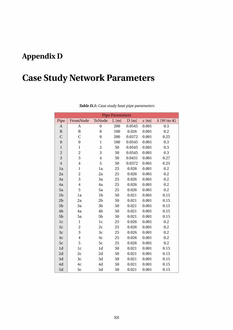
Appendix D
Case Study Network Parameters
Table D.1: Case study heat pipe parameters
Pipe ParametersPipe FromNode ToNode L [m] D [m] ε [m] λ [W/m-K]
A A 0 200 0.0545 0.001 0.3B B 0 100 0.026 0.001 0.2C C 0 200 0.0372 0.001 0.250 0 1 100 0.0545 0.001 0.31 1 2 50 0.0545 0.001 0.32 2 3 50 0.0545 0.001 0.33 3 4 50 0.0431 0.001 0.274 4 5 50 0.0372 0.001 0.25
1a 1 1a 25 0.026 0.001 0.22a 2 2a 25 0.026 0.001 0.23a 3 3a 25 0.026 0.001 0.24a 4 4a 25 0.026 0.001 0.25a 5 5a 25 0.026 0.001 0.21b 1a 1b 50 0.021 0.001 0.152b 2a 2b 50 0.021 0.001 0.153b 3a 3b 50 0.021 0.001 0.154b 4a 4b 50 0.021 0.001 0.155b 5a 5b 50 0.021 0.001 0.151c 1 1c 25 0.026 0.001 0.22c 2 2c 25 0.026 0.001 0.23c 3 3c 25 0.026 0.001 0.24c 4 4c 25 0.026 0.001 0.25c 5 5c 25 0.026 0.001 0.21d 1c 1d 50 0.021 0.001 0.152d 2c 2d 50 0.021 0.001 0.153d 3c 3d 50 0.021 0.001 0.154d 4c 4d 50 0.021 0.001 0.155d 5c 5d 50 0.021 0.001 0.15
XII

Table D.2: Case study heat network parameters
Network ParametersParameter Variable ValueSupply temperature Ts 70 °CReturn temperature Tr 40 °CAmbient temperature Ta 10 °CReference Node Pressure Ps 800,000 Pa
(82.48 m head)
Table D.3: Case study heat loads
Node LoadsNode ΦSP [W] Node ΦSP [W] Node ΦSP [W]
1a 20,000 1c 20,000 A -321,5052a 20,000 2c 20,000 B -50,0003a 20,000 3c 20,000 C -68,4954a 20,000 4c 20,000 05a 20,000 5c 20,000 11b 20,000 1d 20,000 22b 20,000 2d 20,000 33b 20,000 3d 20,000 44b 20,000 4d 20,000 55b 20,000 5d 20,000
Table D.4: Case study electric line parameters
Line ParametersLine FromBus ToBus L [km] R [Ω/km] X [Ω/km] CCL [nF/km]
A A 00 0.3 0.164 0.080 100B 00 B 0.3 0.164 0.080 100C B C 0.2 0.164 0.080 1001 0 1b 0.05 0.164 0.080 1002 1b 2b 0.05 0.164 0.080 1003 2b 3b 0.05 0.164 0.080 1004 3b 4b 0.05 0.164 0.080 1005 4b 5b 0.05 0.164 0.080 1006 5b 5a 0.05 0.164 0.080 1007 5a 5c 0.05 0.164 0.080 1008 5c 5d 0.05 0.164 0.080 1009 5d 4d 0.05 0.164 0.080 100
10 4d 3d 0.05 0.164 0.080 10011 3d 2d 0.05 0.164 0.080 10012 2d 1d 0.05 0.164 0.080 10013 5a 4a 0.05 0.164 0.080 10014 4a 3a 0.05 0.164 0.080 10015 3a 2a 0.05 0.164 0.080 10016 2a 1a 0.05 0.164 0.080 10017 5c 4c 0.05 0.164 0.080 10018 4c 3c 0.05 0.164 0.080 10019 3c 2c 0.05 0.164 0.080 10020 2c 1c 0.05 0.164 0.080 100
XIII APPENDIX D. CASE STUDY NETWORK PARAMETERS

Table D.5: Case study electric network parameters
Network ParametersParameter Variable ValueBase S Sbase 0.010 MVABase V (MV) Vbase,MV 10 kVBase V (LV) Vbase,LV 0.4 kVFrequency F 50 Hz
Table D.6: Case study electric loads (all power factors cos(θ) are lagging)
Node LoadsBus P SP [MW] cos(θ) Bus P SP [MW] cos(θ) Bus P SP [MW] cos(θ)1a 0.003 1.0 1c 0.003 1.0 A -0.0198122a 0.003 1.0 2c 0.003 1.0 B 0.052688 0.903a 0.003 1.0 3c 0.003 1.0 C -0.01254a 0.003 1.0 4c 0.003 1.0 005a 0.003 1.0 5c 0.003 1.0 01b 0.003 1.0 1d 0.003 1.02b 0.003 1.0 2d 0.003 1.03b 0.003 1.0 3d 0.003 1.04b 0.003 1.0 4d 0.003 1.05b 0.003 1.0 5d 0.003 1.0
APPENDIX D. CASE STUDY NETWORK PARAMETERS XIV

Appendix E
Case Study Load Flow Results
Table E.1: Case study heat node results
Heat Node ResultsCHEsim Hsim
Node Ts [°C] Tr [°C] h [m] Φq [W] Ts [°C] Tr [°C] h [m] Φq [W]A 70.0 39.374 82.481 -303,174 70.0 39.375 82.481 -306,078B 70.0 39.217 81.192 -54,064 70.0 39.221 81.168 -54,581C 70.0 38.93 77.298 -73,037 70.0 38.899 76.732 -69,6130 69.446 39.552 73.133 0 69.446 39.552 72.952 01 69.319 39.615 63.798 0 69.319 39.615 63.618 02 69.24 39.626 60.795 0 69.24 39.626 60.615 03 69.135 39.644 59.093 0 69.135 39.644 58.913 04 68.993 39.67 56.402 0 68.994 39.67 56.221 05 68.734 39.737 54.891 0 68.734 39.737 54.711 0
1a 69.106 39.839 62.534 20,000 69.106 39.839 62.354 20,0002a 69.028 39.839 59.524 20,000 69.028 39.839 59.343 20,0003a 68.924 39.84 57.813 20,000 68.924 39.84 57.633 20,0004a 68.784 39.841 55.109 20,000 68.784 39.841 54.929 20,0005a 68.527 39.842 53.576 20,000 68.527 39.842 53.395 20,0001b 68.478 40.0 60.457 20,000 68.478 40.0 60.277 20,0002b 68.402 40.0 57.436 20,000 68.402 40.0 57.256 20,0003b 68.302 40.0 55.710 20,000 68.302 40.0 55.530 20,0004b 68.166 40.0 52.986 20,000 68.166 40.0 52.806 20,0005b 67.918 40.0 51.415 20,000 67.918 40.0 51.235 20,0001c 69.106 39.839 62.534 20,000 69.106 39.839 62.354 20,0002c 69.028 39.839 59.524 20,000 69.028 39.839 59.343 20,0003c 68.924 39.84 57.813 20,000 68.924 39.84 57.633 20,0004c 68.784 39.841 55.109 20,000 68.784 39.841 54.929 20,0005c 68.527 39.842 53.576 20,000 68.527 39.842 53.395 20,0001d 68.478 40.0 60.457 20,000 68.478 40.0 60.277 20,0002d 68.402 40.0 57.436 20,000 68.402 40.0 57.256 20,0003d 68.302 40.0 55.710 20,000 68.302 40.0 55.530 20,0004d 68.166 40.0 52.986 20,000 68.166 40.0 52.806 20,0005d 67.918 40.0 51.415 20,000 67.918 40.0 51.235 20,000
XV

Table E.2: Case study heat pipe flows
Heat Pipe FlowsCHEsim Hsim
Pipe m [kg/s] m [kg/s]A 2.368 2.390B 0.420 0.424C 0.562 0.5350 3.350 3.3501 2.685 2.6852 2.019 2.0193 1.350 1.3504 0.678 0.678
1a 0.332 0.3322a 0.333 0.3333a 0.334 0.3344a 0.336 0.3365a 0.339 0.3391b 0.168 0.1682b 0.168 0.1683b 0.169 0.1694b 0.170 0.1705b 0.171 0.1711c 0.332 0.3322c 0.333 0.3333c 0.334 0.3344c 0.336 0.3365c 0.339 0.3391d 0.168 0.1682d 0.168 0.1683d 0.169 0.1694d 0.170 0.1705d 0.171 0.171
APPENDIX E. CASE STUDY LOAD FLOW RESULTS XVI

Table E.3: Case study electric bus results
Electric Bus ResultsCHEsim Esim
Bus |V | [V] δ [deg] P [W] Q [VAr] |V | [V] δ [deg] P [W] Q [VAr]A 10000.000 1.000 -19366 -45806 10000.000 -0.003 -24113 -35677B 9999.886 1.000 13986 4597 9999.888 -0.001 12500 6054C 10000.000 1.000 -55614 43242 10000.000 0.000 -49380 3165600 9999.794 1.000 0 0 9999.795 -0.003 0 00 399.992 1.000 0 0 399.992 -0.003 0 0
1a 392.778 0.967 3000 0 392.778 -0.506 3000 02a 392.841 0.968 3000 0 392.841 -0.501 3000 03a 392.966 0.968 3000 0 392.966 -0.493 3000 04a 393.154 0.970 3000 0 393.154 -0.479 3000 05a 393.404 0.971 3000 0 393.404 -0.461 3000 01b 398.737 0.995 3000 0 398.737 -0.089 3000 02b 397.545 0.989 3000 0 397.545 -0.171 3000 03b 396.416 0.984 3000 0 396.416 -0.250 3000 04b 395.349 0.980 3000 0 395.349 -0.324 3000 05b 394.345 0.975 3000 0 394.345 -0.395 3000 01c 392.150 0.964 3000 0 392.150 -0.551 3000 02c 392.212 0.965 3000 0 392.212 -0.546 3000 03c 392.338 0.966 3000 0 392.338 -0.537 3000 04c 392.526 0.967 3000 0 392.526 -0.524 3000 05c 392.777 0.969 3000 0 392.777 -0.506 3000 01d 391.835 0.964 3000 0 391.835 -0.573 3000 02d 391.898 0.965 3000 0 391.898 -0.568 3000 03d 392.024 0.965 3000 0 392.024 -0.560 3000 04d 392.212 0.966 3000 0 392.212 -0.546 3000 05d 392.463 0.967 3000 0 392.463 -0.528 3000 0
XVII APPENDIX E. CASE STUDY LOAD FLOW RESULTS

Table E.4: Case study electric line currents
Electric Line ResultsCHEsim Esim
Line |I | [A] θ f r om [deg] θto [deg] |I | [A] θ f r om [deg] θto [deg]A 5.017 -67.086 112.498 4.345 -55.949 123.361B 6.259 -131.978 48.596 5.197 -135.581 45.157C 7.025 -142.539 37.866 5.849 -147.857 32.6631 152.482 -0.452 179.548 152.482 -0.451 179.5482 144.958 -0.471 179.529 144.958 -0.471 179.5293 137.412 -0.488 179.512 137.412 -0.487 179.5134 129.844 -0.502 179.498 129.844 -0.501 179.4985 122.256 -0.513 179.486 122.256 -0.513 179.4876 114.648 -0.521 179.478 114.648 -0.521 179.4797 76.483 -0.540 179.460 76.483 -0.539 179.4608 38.257 -0.551 179.448 38.257 -0.550 179.4499 30.613 -0.558 179.441 30.613 -0.557 179.442
10 22.964 -0.563 179.435 22.964 -0.562 179.43611 15.311 -0.567 179.431 15.311 -0.566 179.43212 7.656 -0.569 179.426 7.656 -0.568 179.42713 30.539 -0.491 179.508 30.539 -0.490 179.50914 22.909 -0.496 179.502 22.909 -0.495 179.50315 15.275 -0.500 179.498 15.275 -0.499 179.49916 7.638 -0.502 179.493 7.638 -0.501 179.49417 30.588 -0.535 179.463 30.588 -0.535 179.46418 22.946 -0.541 179.458 22.946 -0.540 179.45819 15.299 -0.544 179.453 15.299 -0.544 179.45420 7.650 -0.547 179.449 7.650 -0.546 179.449
APPENDIX E. CASE STUDY LOAD FLOW RESULTS XVIII