electrical power systemmodeling and simulation of putrajaya
TRANSCRIPT

Electrical Power System Modeling and Simulation of Putrajaya
Precinct 5 Gas District Cooling Plant
by
Nurul Nashwar binti Mohd Taib
Dissertation submitted in partial fulfillment of
the requirements for the
Bachelor of Engineering (Hons)
(Electrical and Electronics Engineering)
DECEMBER 2004
Universiti Teknologi PETRONAS
Bandar Seri Iskandar
31750 Tronoh
Perak Darul Ridzuan

CERTIFICATION OF APPROVAL
Electrical Power System Modeling and Simulation of Putrajaya
Precinct 5 Gas District Cooling Plant
by
Nurul Nashwar binti Mohd Taib
A project dissertation submitted to the
Electrical andElectronics Engineering Programme
Universiti Teknologi PETRONAS
in partialfulfillment of the requirement for the
BACHELOR OF ENGINEERING (Hons)
(ELECTRICAL AND ELECTRONICS ENGINEERING)
Approved by,
(Mr. Zuhairi B Hj Baharudin)
UNIVERSITI TEKNOLOGI PETRONAS
TRONOH, PERAK
December 2004

CERTIFICATION OF ORIGINALITY
This is to certify that I am responsible for the work submitted in this project, that the
original worki s my ownexcept ass pecified in the references and acknowledgements,
and that the original work contained herein have not been undertaken or done by
unspecified sources or persons.
MOHD TAIB

TABLE OF CONTENTS
CERTIFICATION OF APPROVAL
CERTIFICATION OF ORIGINALITY
ABSTRACT
ACKNOWLEDGEMENT
CHAPTER 1: INTRODUCTION
1.1 Background of Study
1.2 Problem Statement
1.2.1 Problem Identification
1.2.2 Project Significance
1.3 Objectives
1.4 Scope of Study
1.5 Feasibility of Project
CHAPTER 2: LITERATURE REVIEW AND THEORY
2.1 Per Unit Method Short Circuit
2.1.1 Objectives
2.1.2 Per Unit (PU) Notation
2.2 Load Flow Studies
2.3 Overview of SKM® Application Software
in

CHAPTER 3: METHODOLOGY AND PROJECT WORK
3.1 Load Flow Analysis Method 9
3.2 Short Circuit Analysis Method 10
3.3 Developing Model in SKM® Power Tools 11
3.3.1 Switchboard 11
3.3.2 TNB Utility 12
3.3.3 Transformer 13
3.3.4 Cables 15
3.3.5 Induction Machines 18
3.3.6 Distribution Load 21
3.3.7 Protective Devices 23
CHAPTER 4:
CHAPTER 5:
REFERENCES
APPENDICES
RESULTS AND DISCUSSION
4.1
4.2
4.3
4.4
Electrical Equipment Sizing
4.1.1 Transformer Sizing
4.1.2 Cable Rating and Sizing
SKM® Power Tools Report
Data Comparison
26
26
27
29
30
SKM® Power Tools Simulation Studies Diagram 35
4.4.1 Comprehensive Short Circuit Study
Simulation Diagram 35
4.4.2 Load Flow Study Simulation Diagram 36
CONCLUSION AND RECOMMENDATION 38
41
42

LIST OF FIGURES
Figure 1: Radial System Losses
Figure 2: Single Line Diagrams for Basic EngineeringDesign
Figure 3: SingleLineDiagrams for Detail Engineering Design
Figure 4: Load Flow Analysis
Figure 5: Comprehensive Short Circuit Study
Figure 6: Switchboard Component Editor
Figure 7: Utility Component Editor
Figure 8: Transformer Component Editor (2-Winding Transformer)
Figure 9: Transformer Component Editor (Transformer Impedance)
Figure 10: TransformerComponent Editor (Automatic LTC)
Figure 11: TransformerComponent Editor (Damage Curve)
Figure 12: Cable Component Editor (Cable)
Figure 13: Cable Component Editor (Cable Z Matrix)
Figure 14: Cable Component Editor (Impedance)
Figure 15:Cable Component Editor (Damage Curve)
Figure 16: Motor Component Editor (Induction Motor)
Figure 17: Motor Component Editor (Induction Motor-FLA Calculator, Power Factor and
Efficiency)
Figure 18: Motor Component Editor (Motor Diversity)
Figure 19: Motor Component Editor (Motor Diversity-Rated HP)
Figure 20: Motor Component Editor (IEC Contribution)
Figure 21: Motor Component Editor (TCC Starting Curve)

Figure 22: Motor Component Editor (TCC StartingCurve)
Figure 23: Distribution Load Component Editor (General Load)
Figure 24: Distribution LoadComponent Editor (LoadDiversity)
Figure 25: Air CircuitBreakerComponent Editor (Protective Device)
Figure 26: Vacuum CircuitBreaker Component Editor (Protective Device)
Figure 27: Capacitor Bank Component Editor (Protective Device)
Figure 28: Bus-tie Component Editor
Figure 29: Study Selection and Setup Screen
Figure 30: Voltage Drop
LIST OF TABLES
Table 1: Load Demand Estimation
Table 2: Calculation Results for Transformers
Table 3: Parameter Settings for Both Simulation Analyses
Table 4: Data Comparison for Fault ContributionReport
Table 5: Data Comparison for Load Flow SummaryReport

LIST OF EQUATIONS
Equation 1: Zpu = kVABaSe / kVAutiiityPuQ
Equation 2 : ZpU =X"d (kVMotor / kVBase f (kVABase / kVAMotor) puQ
Equation 3 : ZpU =ZCable / (kVBaSe2* 1000 / kVABase) puQ
Equation 4 : Zpu = (ZTransfom1er%)*(kVTranSformer)2*(kVABase) puO
Equation 5 : IShort circuit = (V / Z^^nm) puA
Equation 6 : Ishort circuit = Ishort circuit pU*IBase
Equation 7 : IBase = kVABase / 31/2*kVBase
Equation8:I = P+jQ/E2*
Equation 9 : Vd = I(R+jX)
Equation 10: E2 = (Er] - IR) + j(Eu - IX)
Equation 11: (Ratedmotor) / (3 lA *voltage*power factor*efficiency)
Equation 12: I2t
Equation 13: (Let through energy of fuse) / (Cable S.C. withstand capacity)*100%

ABSTRACT
As a prerequisite for FYP, the author is required to submit a dissertation that records on
going study of electrical power system in a Gas District Cooling (GDC) Plant located in
Putrajaya Precinct 5, which subsequently is simulated to explore the system behaviour
and response. Two major approaches of power system analysis, which has been covered,
are load flow and short circuit studies. In relation with the operation of the plant, it is
necessary to conduct such studies to ensure system's stability and robustness.
The robustness of a power system is measured by the ability of the system to operate in a
state of equilibrium under normal and perturbed conditions. Power system stability deals
with the study of power system's behaviour under conditions such as sudden changes in
load or short circuits on buses or branches.
The first section of this report will elaborate on the introductory part, which consists of
the brief description on the project, the scope of work and also the main activities that the
author has participated.
The second part of the report will cover the details of the literature review that the author
has undergone. The first study being carried out is the process requirements, which
encompass mechanical principles of the GDC system that is very important in designing
Electrical Load Analysis (ELA). ELA is then evaluated to calculate maximum demand
and peak load. Equipment sizing, power flow study using Newton-Raphson method and
short circuit study using Per Unit method based on comprehensive study has also been
conducted.

The third section will focus on the methodology that has been taken by the author
throughout her final year period in UTP. Consequently, this section will highlight
procedures and tools that have been utilized in
SKM® Power Tools [4]. SKM® Power Tools [4] have been extensively used in industry
as it usually has the simplest solution for most cases. The aim of this project is to
understand how the system works by creating a software simulation that represents
electrical power utilization. Prior to this, there is a need in understanding an electrical
system response with presence of a disturbance and interruption.
This next slot represents results and discussion that has been covered especially on short
circuit and load flow studies. The main intention is to develop a model for load flow and
short circuit studies to validate the accuracybased on the relevant data obtained from the
plant.
The last section will outline some recommendations and will represent as conclusion of
the report. This chapter is focusing on the relevancy of this study and the achievement of
this project according to the objective and mile stone set that can be made out of this
project for the next project's development.
n

ACKNOWLEDGEMENT
Sir Isaac Newton once said, "If I have seen farther from other men, it is because I have
stoodon the shoulders of giants." I am most grateful to all personnel whose works I have
drawn from them. They are the giants on whose shoulders I stood while working for my
final year project. Upon completing the two semesters of my final year project, I would
like to express my deepest appreciation, first and foremost to ALLAH, The Al-Mighty,
for giving me the strength andperseverance to undertake all the tasks assigned.
Millions of thanks are specially dedicated to my supervisor, Mr. Zuhairi bin Haji
Baharudin, for his support and enthusiasm throughout my final year semesters. I have
discovered that a major project like this is a formidable task. Whenever I stumbled on
problems during the course, he gave me the chance to think out of the box and assist me
in solving the problems critically. My utmost gratitude aptly is also dedicated to the
management of Electrical Department in Oil, Gas & Petrochemical Technical Services
Sdn. Bhd, for helping me in obtaining all the data required for my project especially Ir.
Zakariya Ibrahim, Electrical Manager of Engineering Division and my training
supervisor, Puan Adita JoharaMat Husin for their unfailing assistance.
Last but not least, I wish to pay tribute to my family, especially my parents, Tn Dr. Haji
Mohd Taib bin Haji Hashim and Mrs. Hajah Mazhariah binti Mansor for their
encouragement and tolerance in many ways during my final year project period. And also
to my friends, who shared their ideas, experiences and encouragement.
Thank you
May ALLAH SWT bless all ofyou.
in

CHAPTER 1
INTRODUCTION
1.1 Background of Study
The emphasis is on the consideration of the system as a whole rather than on the
engineering details of its constituents. According to S.Mattson (1998), modern electric
power systems are themost complex large-scale technical systems developed bymankind
since its main goal is providing continuous power supply to the facility with little or no
interruptions [1]. The power supply for GDC Plant is obtained from llkV feeder of
Tenaga Nasional Berhad (TNB) supply for Phase 1. The computation for various buses
and interconnecting lines are as follows, starting from down-stream loads at 415V
Switchgear/MCC buses A andB that are supplied from 11/0.415-TxlAand 11/0.415-
TxlB respectively. These ll/0.415kV transformers are supplied at llkV from the llkV
Switchboard buses. Similarly, the 3.3kV Switchgear/MCC buses A and B are supplied by
1l/3.3kV power transformers; 11/3.3-TxA and 11/3.3-TxB respectively, which in turnare
fed from the llkV Switchboard buses. 33kV feeder is going to be tapped during
development of Phase 2 onwards due to the additional of future loads. The study analysis
that has been carried out is based on the power intake taken at llkV to cater for the
present estimated loads. Distributions of electrical power to various loads of the plant via
different buses are as follows: -
• 1IkV Switchboard Bus A and B (Phase 1)
• 3.3kV Switchgear/MCC Bus A and B (Phase 1 to Phase 4), as the ll/3.3kV step
downtransformers has to be purchased at Phase 1 of the project
• 415V Switchgear/MCC Bus A and Bus B (Phase 1)

The anticipated maximum demand for all phases of the plant is approximately 7.5MVA
during basic engineering design. Additional equipment during detail engineering design
leads to increment in load demand up to 9.0MVA. Phase wise approximate load demand
estimated is as shown below: -
Table 1: Load Demand Estimation
Description Year Basic EngineeringDesign
Detail EngineeringDesign
Phase 1 2004 3.4 MVA 4.8 MVA
Phase 2 2007 1.7 MVA 1.8 MVA
Phase 3 2008 1.4 MVA 1.4 MVA
Phase 4 2012 1.0 MVA 1.0 MVA
1.2 Problem Statement
"Electrical Power System Modeling and Simulation"
"Electrical Power System" defines a set of complete electrical network that consists of all
the electrical distribution panels and loads at certain level of voltage rating. "Modeling"
here refers mathematical representation of electrical motor and non-motor various loads.
"Simulation" is defined as generation of tests on a virtual-time basis to predict the short
circuit behavior and load flow analysis of the real system. Computer-aided tool that will
be used is SKM® Power Tools [4]; an electrical engineering software.
1.2.1 Problem Identification
Electrical Engineers need to perform specific study to avoid fault current from occurring
and load flow study to determine power consumption. Accurate load flow and short
circuit is of great importance for power system operation to be stable under any
circumstances and conceivable disturbances. Disturbances in industrial power systems
are large in magnitude and the typical duration of a fault i s t enths of a second. Right
assumptions need to be obtained especially in short circuit and load flow analysis to
simplify calculation. [2]

1.2.2 Project Significance
The results of the analysis can conclude on how much electricity needed by the plant,
how big the equipment will be and what type of protective devices required. The project
can serve as a baseline for modelling of more advanced and complex power systems.
Further expansion plans for the power system in the plant can be facilitated more easily
with the help of the model and simulation. It serves as a starting point for future
undergraduates to acquire more knowledge on power systems and expand the models
developed for further refinement and extended studies.
1.3 Objectives and Scope of Study
• To develop the GDC plant power system model in the SKM® Power Tools [4]
environmentto simulate comprehensive short circuit and load flow studies
• To specify losses for all busses
• To obtain the switchgear rating and size of capacitor banks
The scope of study will be narrowed to a specific section in the GDC Plant where the
electrical loads are concern. Continuous loadwill be the major type of load to be studied
followed by Intermittent Load and Stand-by Load. The power system that covers all
important elements andcomponents will be modelled and simulated to predict the system
performance and manners. Comprehensive studies based on per unit method for short
circuit simulation and Newton-Raphson method for load flow analysis is the major
concern involved.
1.4 Feasibility of Project
Supported data on electrical power system obtained from the engineering consultant
company should be adequate to view general concept of the electrical components of the
system and to impart all the required data for the analysis. The availability o f S KM®
Power Tools [4] software in the laboratoryproved to be helpful and the project is feasible
to be carried out within the given time and scope.

CHAPTER 2
LITERATURE REVIEW / THEORY
2.1 Per Unit Method Short Circuit
2.1.1 Objectives
The fault current study canbe evaluated by circuit simplification when all data ratings are
collected and all the impedances are converted to per unit values. Per unit system is
convenient to normalize system variables due to computational simplicity by eliminating
units and expressing system quantities as dimensionless ratios. The objectives of short
circuit currents can be summarized as follows: -
• Determination of short circuit duties on switching devices, i.e., high-, medium- and
low voltage circuit breakers and fuses.
• Evaluations of adequacy of short-circuit withstand ratings of static equipment like
cables, conductors, bus bars, reactors and transformers.
2.1.2 Per Unit (PU) Notation
1) For utility contributions:
ZpU = kVABase/kVAutiiitypuQ Equation 1
Where
• kVA Base = The system three-phase power base specified for the study
• kVA utility = The utility system three-phase short circuit capability

2) For motor and generator contributions:
Zpu =X"d (kVMotor / kVBaSe f (kVABase / kVAMotor) puQ Equation 2Where
• X"d = Motor subtransient reactance
• kV Motor = Line-to-linemotor rated voltage
• kV Base - Line-to-line bus nominal system voltage at the point of the motor
3) For feeders:
Zpu - Zcabie / (kVBase2*1000 / kVABase)puO Equation 3Where
• Zcabie ~ ^er Pnase feeder impedance in ohms
4) For transformers:
Zpu = (^Transformer %)*(kYTransformer) *{kYABase) puQ Equation 4
(100) (kVease)2 (kVATransformer)Where
• Z-rransformer= Transformer % impedance on its self-cooled
The three-phase fault current base is:
Ishort circuit = (V / ZjheveniTi) puA Equation 5
Expressed in Amperes:
Ishort circuit = Ishort circuit pU*lBase Equation 6
Where the base current is defined as:
We=kVABase / 31/2*kVBase Equation 7
2.2 Load Flow Studies
The load flow study is intended to:
• Determine the steady-state loading of the various buses and lines (cables) in the GDC
Plant to ensure that they are operating within their performance ratings
5

• Determine the voltages at the various buses to ensure voltage drops do not exceed
+5% and -10%, consistent with the tap-changer range at the distribution transformers
• Evaluate the amount of capacitive reactive power compensation necessary to bring
the power factor level to 0.93 lagging
The modelling of loads is complicated because a typical load bus is composed of a large
number of devices such as pumps. Consider a simple system as shown in Figure 1. [2]
Source ^•— -*. Busl
Load
Bus 2
P+jQS El R+jX E2
Figure 1: Radial System Losses
The equations relating the above diagram are as follows: -
I = P+jQ/ E2* Equation 8
Where E2 is the voltage conjugate at bus 2. The voltage drop along the line is:
Vd - I(R+jX) Equation 9
Therefore,
E2 = (En - IR) + JCBii - IX) Equation 10
Putting Equations 8 and 10 in another form, three unknowns are existed as follows:
I = Ir+ jlj, E2 = Er2 + jE2i and (E2* = Er2 + jE2i)
Equations above can be solved by iterative technique, Newton-Raphson.
2.3 Overview of SKM® Application Software
SKM® Power Tools [4] offers a full spectrum of analysis capabilities such as: -
• I*SIMTransient Stability - to evaluate performance and stability of power system
• HarmonicAnalysis - to simulate harmonic content and distribution
• DAPPER balanced system studies - to simulate load flow and short circuit studies.
The sub-tool that will be concentrated is DAPPER Balanced System Study.
Single line diagrams drawn in SKM® Power Tools for basic and detail engineering
design of Putrajaya Precinct 5 GDC Plant are as shown in Figure 2 and Figure 3.

llk
VS
to
ard
I1
/D
.41
5T
xlA
41
5V
Bu
s1
41
5V
Ph
ase
1
GD
CP
RE
CIN
CT
5D
IS
TR
IC
TC
OO
LIN
GP
LA
MT
TN
B1
1k
V(P
hase
1-
Ph
ase
2)
3.3
kV
Ph
asel
3.3
kV
Fu
tu
re
3.3
kV
Bu
s2
Fig
ure
2:Si
ngle
Lin
eD
iagr
amfo
rB
asic
Eng
inee
ring
Des
ign
1I
A)
.41
5T
jcIB
11
/4
15
b2 4
15
VB
us2
41
SV
Ph
asel

-S—- -©5
HHi'
-=«r
H®
HHi.
& -a—- -®5
§ I--© •
-©
-©5
HB' 2
-©I
-Gl
-Q3
-H3g
-®3
-©s
-© =
~© =
-05
HHm
-©E
-®=
~-®s
-©I
360
• i—•
«
Qbog
00a
wo
• 1—1
ffl
&
fl• i—i
s,"Bo
oo

CHAPTER 3
METHODOLOGY/PROJECT WORK
Literature reviews on books and journals are accomplished throughout the early stage.
Apart from that, the author has chosen a case study for a better understanding in real
application. The next step is to simulate the electrical power system using appropriate
power analysis software. Suggested milestone forwhole year is shown in APPENDIX 1.
3.1 Load Flow Analysis Method
Load flow steps in SKM® Power Tools [4] are illustrated as below: -
Define System DataDefine system topology and connectionsDefine utility connections (swing bus)
Define individual loads
Define feeder and transformer sizes
Define generator sizes
Run Load Flow Study
Saved in Database
For each branch
Voltage dropPower flow
Study Setup For each bus
Cable LibraryTransformer Library
VoltageVoltage anglew
Demand Loads Voltage dropConnected Loads Power flow
Study Setup Power factor
i
,-^rir-ti
x^g^^fii
*fe=£«
Figure 4: Load Flow Analysis Flow Chart
Report

In order to come out with ELA, process and mechanical equipment data need to be
analysed first since it plays myriad roles to meet the required demand and conditions of
the GDC Plant. The absorbed load for all equipments will be converted to electrical load
using certain formulas. Overall process flow diagram is as shown in APPENDIX 2.
Demand load and connected load can be determined from ELA, shown in APPENDIX 3
for both basic and detail engineering design.
3.2 Short Circuit Analysis Method
Figure 5 below shows procedures in SKM® Power Tools [4] .to develop comprehensive
short circuit study.
•>
;lio-$
semis awtyc&rmecilon i>w!ng b«3<
Dafhis %d\ coairbuiior
•"•d.^iiiirj3**g:;;^
!un Short Circuit Study
Saved in Database
leal ftuilt currents
Figure 5: Comprehensive Short Circuit Study Flow Chart
10

Comprehensive short circuit study models the current that flows in the power system
under abnormal conditions and determines the prospective fault currents in an electrical
power system. [3]. Comprehensive short circuit analysis procedure involves reducing the
network at the short circuit location to a single Thevenin equivalent impedance,
determining the associated fault point R/X ratio calculated using complex vector algebra
and defining a driving point voltage (assuming the effect of the transformer taps on bus
voltage).
3.3 Developing Model in SKM® Power Tools [4]
In developing model for analysis in SKM® Systems Analysis [4], design specifications
and descriptions of all major equipments need to be verifiedfirst as depicted below: -
3.3.1 Switchboard
The switchboard is designed for each voltage rating. An example of switchboard buses
component editor that displays essential data to be entered is as shown in Figure 6.
Component Sub"iew;
Hatmonic SoMfce
3.3RV busl
•33kVS*boa;dA
•415V Bus1
»41$VE*$ent!sS
""SUS-0030
"•BUS-Q031
tlWJtSwdA
' :• fU\ •:::»'
Figure 6: Switchboard Component Editor
11

3.3.2 TNB Utility
TNB Utility is designed based on Tenaga Nasional Berhad's (TNB's) requirement.
Supplymay be provided at any of the declared voltages: -
Low Voltage
1. Single-phase, two-wire, 240V, up to 12kVAmaximum demand
2. Three-phase, four-wire, 415V, up to 45kVA maximum demand
3. Three-phase, four-wire, C.T. metered, 415V, up to 1500kVAmaximum demand
Medium Voltage andHigh Voltage
1. 3-phase, 3-wire and 1lkV for load of 1.5MVA maximum demand and above
2. 3-phase, 3-wire, 22kV and 33kV for load of 5MVA maximum demand and above
3. 3-phase, 3-wire, 66kV, 132kV and 275kV for exceptionally large load of above
20MVA maximum demand
Data from TNB that has been included in SKM® Power Tools [4] is 3-phase, 3-wire and
1lkV as shown in utility component editor in Figure 7.
Component Subviem.
Harmonic lmp@<Reliable Data
« Manager.,,_
Name: TN8
r InWai 3peratingCortcKom—
Voit§ge: 1.000 pu
» Enter
Utility Contribution
iins to Ground:
-Per Unit Contribution
Base/RatedMoitage (L-LJ;
ft. ... X100.0 gositive
2ero
0.327861 0.010819
11000 1000000 1000000 '
Bus: BUS-004S
Figure 7: Utility Component Editor
12

3.3.3 Transformer
Transformers shall be connected in parallel, where each transformer capacity shall be
adequate to carry all the loads connected via bus-tie in case of failure or maintenance of
either of transformers (100% redundancy). All the data required to be entered for
transformer is as shown in 11/0.415kV transformer component editor in Figure 8 to
Figure 11. Pop-menu windows for component sub views as listed below will not be
shown since all the data need not to be entered as it is automatically calculated by SKM®
Power Tools [4]: -
• Reliability Data
• User-Defined Fields
• Datablock
j3usVoitage:
11000 V(L-L3
VMJ
433
1 \ UD0 415
•84,0 l2f3£T0.00 0.00
Full Load Amps: -B4.0
VMJ
Pos. Seq. Pri. Voltage;ieads Sec.
• Bus Qsnnection ••—"'••-,"™"™"*™s
30.0 Link Phas« SWft
| From: BUS-0050
i To: BUS-005?
Mid Tap
L4L-&
Ts jL'0.-j!5 A
lCB!
Figure 8: Transformer Component Editor (2-Winding Transformer)
13

2-WJndingTransformef
icLTC
Go To j£_ Jump... j
£ero:
0,0060 6.0Q0Q
0,0060 aoooo
R(Ohffns) XtOhms)
O00000 0.00000 Cafe...
0,00000 aoaooo Calc.
•No Loadtoss in Percent en Transformer Bass
0.0000 jo.ooea
IEC Format 2-..
P Do NotSize
Siang Criteria;
Transformer 8a
** Nomina) k'
r FullLoad!
Uit-i!
«M-
w CBL-
Figure 9: Transformer Component Editor (Transformer Impedance)
Component Sybyiews.LTC isonly available with thesingle-phase / unbalanced 3-phase IF
le Tap Bus; jf';:> Vit> jj
:ledQuantity Limits ™' •• -— - - — -••••'• >
f Tap Limit
! Max, Tap:
P-U- \" Controlled'Phase:
p.u. | |i "CjP-u. [ „_
wwmf
w CBU
Figure 10: Transformer Component Editor (Automatic LTC)
14
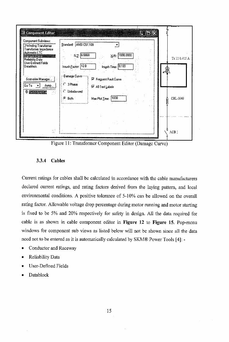
2-Windtng TransformerTransformer ImpedanceAutomatic LTC
Standard: jANS! C57.109"" —'•*••*•"•—"•"••—<
*2 6.0000 JS/R: 1000.0000
Inrush Eactor: 110 IniyshTime: aioo
r Damage Curve—.; I W Freguent FauStCurve
jf" 3Phase j pAgTexlLabefeIf" Unbalanced j
\& Bo\h 1 Max Ptot lime: ^00
Tsn.'0,4nA
ACB
Figure 11: Transformer Component Editor (Damage Curve)
3.3.4 Cables
Current ratings for cables shall be calculated in accordance with the cable manufacturers
declared current ratings, and rating factors derived from the laying pattern, and local
environmental conditions. A positive tolerance of 5-10% can be allowed on the overall
rating factor. Allowable voltage drop percentage during motor running and motor starting
is fixed to be 5% and 20% respectively for safety in design. All the data required for
cable is as shown in cable component editor in Figure 12 to Figure 15. Pop-menu
windows for component sub views as listed below will not be shown since all the data
need not to be entered as it is automatically calculated by SKM® Power Tools [4]: -
• Conductor and Raceway
• Reliability Data
• User-Defined Fields
• Datablock
15

Damage CurveReliability DataUser-Defined Fi
Goto "
Figure 12: CableComponent Editor (Cable)
m^-mmm
R iX
A 0,007328 10.007713
8 P.
C o.
From: BUS 0044
To: 33kVS;GA
R ' J0.
kcemT Iabo77f3" Eolio " 15
aoooooo o.
QK
TxVHJ;
•121
Figure 13: Cable Component Editor (Cable Z Matrix)
16
vcs:
C8L-2
, Tall.
C3L-*
\VC8-
*'C tt
?'JU

Conductor and IDamage Curve
Datablock
Go To »
•r-rrs
0.0738 0.0840
0.0798 0.0840
lUance-™- "'•"'-
G/2 8/2
0.000000 0.000000
0.000000 0.000000 \ ITS•
(Ms: Mhos/1000 Meiers
"Jt'iiOTUira #^12
Figure 14: Cable Component Editor (Impedance)
p Cable Plot— ^
| * Single CParafel r $\| Conductors in Parailal(,iPhase:
r CableAmpact^-"-
& C,alculaiedAmpacity
1 r Load FfDW Current
j Ampacity. 5.0 (DesignAmpadSy is 0)
gqr!«war«w»
JC2 JVC.10,
Ts\TD.i
:[oui
Figure 15: Cable Component Editor (Damage Curve)
17
C3i>
?-oi

3.3.5 Induction Machines - Motor Load
Induction motors are calculated based on maximum demand as shown below from
Figure 16 to Figure 22. Pop-menu windows for component sub views as listed below
will notbe shown since all the data need not to be entered as it is automatically calculated
by SKM® Power Tools [4]:-
• Harmonic Source
• Reliability Data
• Load Profiles
• User-Defined Fields
• Datablock
P-IUU
Figure 16: MotorComponent Editor (Induction Motor)
18

Motor Diversity!EC ContributionTCt Starting CurveTransient MotorStartirHarmonic Source
Load ProfileUser-Defined Fields
|GoTo jrj Jump...
Number ofM<3*°fs: 2
Rated Voit§ge: 415
Rated Size: 0,40
Power Factor; 0.8500
Efficiency l.POQO
Pojes: p
Figure 17: MotorComponent Editor (Induction Motor-FLA Calculator, Power Factorand
Efficiency)
TCC$i§!tiy*3tifivi i
MMni</ Data
Scenarios Manage!
jii*4» flmrf
Figure 18: Motor Component Editor (Motor Diversity)
19

EC ContributionTCC Starting CurveTransient Motor Starts?Harmonic Source
Load Factor
•J.iii.i.11,^ j, «aM.,>w.
BHR 10.482574
i- wwtgi' wwiM p-
•tfj. . . i».>j»«.^.jeL..m.
:-9wm
OSOaA 9*112 U F412IS
®p-nuA
Figure 19: MotorComponent Editor (MotorDiversity-Rated HP)
So To "* *> lit*, waited
RtGhrx) X
ISC $12630*4
?;4irB**Btar*w/Roi*Rwci«««w *1 tUtfl J
?<T [18C? #» tdc 11/3 irt.
Figure 20: Motor ComponentEditor (IEC Contribution)
20
(s

GoTo »| Aiflas..,
Figure21: MotorComponent Editor (TCC StartingCurve)
£CC0**iU*«i
> It*
Figure 22: Motor Component Editor (TCC Starting Curve)
3.3.6 Distribution Load - Non-motor Load
Distribution loads are non-motor loads such as lighting. The essential data that need to be
entered is as shown in Figure 23 and Figure 24.
21

Pop-menu windows for component sub views as listed below will not be shown since all
the data need not to be entered as it is automatically calculated by SKM® Power Tools
[4]:-
• Harmonic Source
• Reliability Data
• Load Profiles
• User-Defined Fields
• Datablock
Figure 23: Distribution Load Component Editor (General Load)
22

Figure 24: Distribution Load Component Editor (Load Diversity)
3.3.7 Protective Devices
Protective devices are used for power flow control and safe maintenance purposes.
Numbers of protective devices available in industry but only Air Circuit Breakers
(Figure 25), Vacuum Circuit Breakers (Figure 26), Capacitor Banks (Figure 27) and
Bus-Ties (Figure 28) are used in this project. Pop-menu windows for component sub
views as listed below will not be shown since all the data need not to be entered as it is
automaticallycalculated by SKM® Power Tools [4]: -
• Settings
• Reliability Data
• User-Defined Fields
• Datablock
23

Figure 25: AirCircuit Breaker Component Editor (Protective Device)
Figure 26: Vacuum Circuit Breaker Component Editor (Protective Device)
24

ComponentSubview
Figure 27: Capacitor Bank Component Editor (Protective Device)
-oces
Figure 28: Bus-tie Component Editor
25

CHAPTER 4
RESULTS AND DISCUSSION
4.1 Electrical Equipment Sizing
Charles A.Gross (1979) wrote that attempts to model mathematically the electrical power
system for analysis is heavily dependent on circuit concepts [1], Crucial information such
as transformer rating, distribution cable impedance, generator rating is important before
designing the single line diagram in SKM® Power Tools [4].
4.1.1 Transformer Sizing
Table 2: Calculation Results for Transformers
Design Rated
kV
Phase
1
(kVA)
A
Phase
2+3+4
(kVA)
B
Maximum
Demand
Load
(kVA)C-A+B
Size
(kVA)
D=1.25C
Standard
Rated
(MVA)
Basic Engineering 11/
0.415
1253 Future
Stage1253 1563.3 1.6
11/3.3 1836.2 2328.2 4164.4 5205.5 6.0
Detail
Engineering(Without power
factor correction)
11/
0.415
1719 Future
Stage1719 2148.7 2.2
11/3.3 3082 2464 5547 6933 6.95
Detail
Engineering(With power factor
correction)
11/
0.415
1414 Future
Stage1414 1768 1.77
11/3.3 2646 2412 5058 6323 6.325
Transformer kVA size - Maximum demand oad on t le transformer + 5% loss ss + 20%
spare capacity
26

From the table, it is shown that two 11 / 3.3kV transformers at rated size of 6MVA and
two 11 / 0.415kV transformers at rated size of 1.6MVA are used for basic engineering
design. Detail engineering design is encompassed of two 11/ 3.3kV transformers at rated
size of 6.325MVA and two 11 / 0.415kV transformers at rated size of 1.77MVA since the
main focus and interestis on detail engineering designwith power factor correction.
4.1.2 Cable Rating and Sizing
The current carrying capacity is based on the assumption that the ambient temperature is
at 40°C. The cable arrangement diagrams are as shown in APPENDIX 4.
• Sample calculation in determining sizes for high voltage (3.3kV) cables: -
a) Cable ampacity
Cable ampacity derating is taken from the IEE Wiring Regulation book. Cable ampacity
shall be bigger than the motor rated current. In this case, for highest rated pump of
280kW, the rated current after diversity (100%) is 61A.
For example:
The running current of Secondary Chilled Water Pump, P-0101 shall be as follows:-
= (Rated motor) / (3 /z *voltage*power factor*efficiency) - Equation 11
- (280*1000) / (3 '/2 *3300*0.84*0.955) = 61 Ampere
Therefore, cable used shall have ampacity greater than 61A. The cable size to be used
can be as small as 25 sq mm as shown in Table 2 for 3-core cables in APPENDIX 5.
b) Fault level at load terminals
Cables used shall have short circuit (SC) withstand capacity greater than short circuit
level at cable terminal point.
27

However it is safe to use a cable having SC withstand capacity smaller than SC at cable
terminal as long as its SC withstand capacity is greater than let through energy of fuse.
SC withstand capacity of25mm2 cable for 0.2 sec = 8.5kA as shown inAPPENDIX 6.
Therefore, SC withstands energy shall be as follows:-
= 11 Equation 12
- (8.5*103)2A*0.2sec = 1.45*107 Asec
c) Fuse selection:
This is done by referring to fuse selection curves graph for motor starting as shown in
APPENDIX 7. Selection of rated current of the fuse relies on 3 criteria, which are:
• Ia = motor starting current
• Nh = number of motor starts per hour
• TA = maximum starting starting time
In our case:
• IA = 61A x 6 - 366A (Actual vendor data = 400A)
• Nh = 6
• TA = 5s (typical values for DOL started motors)
From the graph, for which the motor run-up times not exceeding 6 seconds, the fuse
rating is 160 A. The maximum let through energy of fuse rating 160A is 50xl04. Let
through energy of the fuse (50xl04 sec) must be less than cable SC withstand capacity
(1.45xl07 Asec) and SC atcable terminal (13.2kA or 1.32xl04). Ratio is as follows:-
= (Let through energy of fuse) / (Cable S.C. withstand capacity)*100% -Equation 13
= (50xl04 A2 sec) / (1.45xl07 A2 sec) * 100%
-3.45%
The ratio implies that the cable SC withstand capacity is 1/0.0345 or 29 times bigger than
the maximum let through energy of the 160A fuse. So, the 25mm cable is well protected
by the 160A fuse. Full result of proposed cables sizes can be referred to APPENDIX 8.
28

4.2 SKM® Power Tools Report
The pop up menu window that show the studies that need to be run is shown below: -
Balanced System Study Setup' *l-iTupias- RsportRie-
*>
15" Q&ffi&nrJLGiifS
r~ -2i7itifj
P7 : oHii Fow
Seiup
rJii fl
Sh*lufi..
Jt rfil
'-P- f" Appgnd
P 5£<? fJowpTo*icrstv,o
• ^ A_FAU.T
r tC9J3B3
ictup... |i
J5C.-'p' r Append |
:,cad Schcctetei rVli p.. r.fi
System I'iCLt Date. Report- Inpjrroi
DefaultRgport Pest D:\PTWV:l5\prcj5Cis\Ty;ori3l-T§*t
tle:p formes.. Header. !I Burt
r .--jjpr.ril
P Append
Cancel
Fig. 31. Study selection and setup screen.
After selecting tke studies, click on the Rim button.
Figure 29: Study Selection and Setup Screen
Comprehensive short circuit study will calculate the initial symmetrical and asymmetrical
short circuit current given the fault location R/X ratios at various times during the onset
of the fault as shown in APPENDIX 9 based on basic engineering design drawing and
APPENDIX 10 based on detail engineering design drawing. Both results are in crystal
report format. Load flow study indicates the apparent power and current at each buses
and within each branches in the electrical power system, excluding local generation and
power lost through impedance devices. Load flow study results in crystal report format
are as shown in APPENDIX 11 based on basic engineering design drawing and
APPENDIX 12 based on detail engineeringdesign drawing.
29

4.3 Data Comparison
To attain maximum power consumption at various switchgear buses, the worst but
practical operational configuration is considered for this study. According to the
consideration:-
• Only one out of two TNB supply is on and supplying all loads to the plant
• Both transformers at each voltage level is supplying power to the entire switchgear
• Bus tie breakers of all switchgear are opened
To get maximum short circuit current at various switchgear buses, the worst but practical
operational configuration is considered for this study. According to that consideration,
• Only one out of two TNB supply is on and supplying all loads to the plant
• Only one out of two transformers at each voltage level is supplying power to the
entire switchgear
• Bus tie breakers of all switchgear are closed
• All motor and non-motor loads are running
The study settings specified for both simulation analyses are as follows: -
Table 3: Parameter Setting 3for Both Simulation Analyses
Short Circuit Study Load Flow Study
• 3-phase fault • Newton-Raphson solution method
• Single-line-to-ground fault • Connected load specification
• Transformer tap and phase shift • Source impedance is included
• Faulted buses at all buses • Generation acceleration factor is 1.00
• Initial symmetrical RMS with lA • Load acceleration factor is 1.00
cycle asymmetrical • Bus voltage drop is 5.00%
• Asymmetrical fault current at time • Branch voltage drop is 3.00%
0.5s
From the simulation results obtained in SKM® Power Tools [4], the below data for both
designs is extracted,compared and summarized.
30

Tab
le4:
Dat
aC
om
par
iso
nfo
rF
ault
Con
trib
utio
nR
epo
rt
Da
taL
oca
tio
nB
asi
cE
ng
inee
rin
gD
esig
nD
eta
ilE
ng
inee
rin
gD
esig
n
Init
ials
ymm
etri
cala
mps
-3P
has
ell
kV
Sw
itch
bo
ard
A1
73
13
A1
58
19
A
llk
VS
wit
ch
bo
ard
B-
15
81
8A
3.3
kV
Bu
s1
17
61
3A
20
05
5A
3.3
kV
Bu
s2
-2
00
41
A
41
5V
Bu
s1
43
78
2A
42
57
8A
41
5V
Bu
s2
OA
42
06
4A
•;.'
"V
-^-.
;,'-
-;-;
?j-
"•,
"i,
'.''-.'
Asy
mm
etri
cala
mp
sSP
ha
sell
kV
Sw
itch
bo
ard
A2
76
41
A1
58
19
A
llk
VS
wit
ch
bo
ard
B-
15
81
8A
3.3
kV
Bu
s1
28
44
6A
24
57
1A
3.3
kV
Bu
s2
-2
45
59
A
4I5
_V
:Bu
s1.."
....
52
18
8.A
52
79
3A
41
5V
Bu
s2
OA
52
33
5A
&£
'^"
*-,:'
--4V*
"•'"-
"4
^;^
->\-
:\-y
-r,.
•
Init
ials
ymm
etri
cala
mp
sSin
gle
Lin
eto
Gro
un
d(S
LG
)
llk
VS
wit
ch
bo
ard
AO
A0
A
1lk
VS
wit
ch
bo
ard
B-
0A
3.3
kV
Bu
s1
17
56
0A
16
55
9A
3.3
kV
Bu
s2
-1
65
48
A
41
5V
Bu
s1
41
13
3A
38
73
0A
41
5V
Bu
s2
OA
38
25
2A
Asy
mm
etri
cala
mps
-Sin
gle
Lin
eto
Gro
un
d(S
LG
)
llk
VS
wit
ch
bo
ard
A
llk
VS
wit
ch
bo
ard
B
3.3
kV
Bu
s1
3.3
kV
Bu
s2
41
5V
Bu
s1
41
5V
Bu
s2
31
OA
28
94
0A
47
98
4A
0A
0A
0A
23
00
1A
22
99
0A
48
93
7A
48
49
0A

Tab
le5:
Dat
aC
ompa
riso
nfo
rL
oad
Flo
wS
umm
ary
Rep
ort
Da
taB
asi
cE
ng
ineeri
ng
Des
ign
Det
ail
En
gin
eeri
ng
Des
ign
TN
BS
ou
rce
Per
Un
itV
olt
age
1.0
01
.00
An
gle
0.0
0°
0.0
0°
Acti
ve
Po
wer
44
51
.0k
W6
10
2.3
kW
Reacti
ve
Po
wer
34
59
.6k
VA
R1
68
1.0
kV
AR
Vo
ltag
eD
rop
1.2
1%
2.1
4%
Uti
lity
Imp
edan
ce0.
01+
J0.3
30.
33+
J0.0
1
Bu
sb
ar
Ao
rB
usb
ar
1
Bu
sb
ar
Bo
rB
usb
ar
2
Bu
sb
ar
Ao
rB
usb
ar
1
Bu
sb
ar
Bo
rB
usb
ar
2
llk
VS
wit
ch
bo
ard
Bu
sb
ar
Vo
ltag
eD
rop
1.2
1%
-2
.14
%2
.14
%
Equ
ival
entt
oB
us
Vo
ltag
e1
08
66
V-
10
76
4V
10
76
4V
An
gle
Deg
ree
-0.8
2°
-0
.26
°0
.26
°
PU
Vo
lts
0.9
9_
0.9
80
.98
Inco
min
gF
eed
erto
Bu
sA
cti
ve
Lo
ad
44
51
.0k
W-
61
02
.3k
W-
Reacti
ve
Lo
ad
34
59
.6k
VA
R-
16
81
.0k
VA
R-
Po
wer
Facto
r0
.79
-0
.96
4-
Lo
ad
Flo
wC
urr
en
t2
63
A-
33
9.2
1A
-
Ou
tgo
ing
Fee
der
fro
mB
us
Acti
ve
Lo
ad
44
50
.6k
W-
60
97
.9k
W-
Reacti
ve
Lo
ad
34
59
.3k
VA
R-
16
67
.5k
VA
R-
Po
wer
Facto
r0
.79
-0
.96
-
Lo
ad
Flo
wC
urr
en
t2
99
.50
A-
33
9.2
1A
-
32

Los
sesf
or
llk
VB
us
*0
.4k
W+
0.3
kV
AR
Bu
sb
ar
Ao
rB
usb
ar
1
Bu
sb
ar
Bo
rB
usb
ar
2
*4
.4k
W+
13
.5k
VA
R
Bu
sb
ar
Ao
rB
usb
ar
1
Bu
sb
ar
Bo
rB
usb
ar
2
3.3
kV
Sw
itch
bo
ard
Bu
sb
ar
Vo
ltag
eD
rop
2.4
7%
2.6
8%
-1.2
1%
-1.5
5%
Eq
uiv
alen
tto
Bu
sV
olta
ge3
21
8V
32
11
V3
34
0V
33
51
V
An
gle
Deg
ree
-31
.78
°-3
1.9
3°
-1.6
8°
-1.1
4°
PU
Vo
lts
0.9
80
.97
1.0
11
.02
Po
wer
Facto
rC
orr
ecti
on
N/A
N/A
90
0k
VA
R7
50
kV
AR
Inco
min
gF
eed
erto
ll/3
.3k
VT
ran
sfo
rmer
Acti
ve
Lo
ad
16
01
.6k
W1
86
2.8
kW
27
18
.5k
W1
97
3.l
kW
Reacti
ve
Lo
ad
12
43
.4k
VA
R1
45
4.3
kV
AR
88
2.7
kV
AR
60
4.5
kV
AR
Po
wer
Facto
r0
.79
0.7
90
.95
0.9
5
Lo
ad
Flo
wC
urr
en
t1
07
.73
A1
25
.57
A1
53
.3A
11
0.6
8A
Ou
tgoi
ng
Fee
derf
rom
ll/3
.3k
VT
ran
sfor
mer
Acti
ve
Lo
ad
16
01
.6k
W1
86
2.8
kW
27
18
.1k
W1
97
2.8
kW
Reacti
ve
Lo
ad
12
01
.2k
VA
R1
39
7.1
kV
AR
78
2.1
kV
AR
55
2.0
kV
AR
Po
wer
Facto
r0
.79
0.7
90
.96
0.9
6
Lo
ad
Flo
wC
urr
en
t3
59
.10
A4
18
.55
A4
88
.8A
35
2.8
9A
Lo
sses
for
3.3
kV
Bu
s*
0k
W+
42
.2k
VA
R*
0k
W+
57
.2k
VA
R
Bu
sb
ar
Bo
rB
usb
ar
2
*0
.4k
W+
10
0.6
kV
AR
*0
.3k
W+
52
.5k
VA
R
Bu
sb
ar
Ao
rB
usb
ar
1
Bu
sb
ar
Ao
rB
usb
ar
1
Bu
sb
ar
Bo
rB
usb
ar
2
33

41
5V
Sw
itch
bo
ard
Bu
sb
ar
Vo
ltag
eD
rop
3.1
7%
3.1
7%
-1.4
1%
-1.0
5%
Equ
ival
entt
oB
usV
olt
age
40
2V
40
2V
42
1V
41
9V
An
gle
Deg
ree
-31
.63
°-3
1.6
3°
-0.9
7°
-1.8
3°
PU
Vo
lts
0.9
70
.97
1.0
11
.01
Po
wer
Facto
rC
orr
ecti
on
N/A
N/A
25
0k
VA
R4
50
kV
AR
Inco
min
gF
eed
erto
ll/0
.41
5k
VT
ran
sfor
mer
Acti
ve
Lo
ad
49
3.l
kW
49
3.l
kW
52
4.8
kW
88
1.5
kW
Reacti
ve
Lo
ad
38
0.8
kV
AR
38
0.8
kV
AR
77
.9k
VA
R1
12
.4k
VA
R
Po
wer
Facto
r0
.79
0.7
90
.99
0.9
9
Lo
ad
Flo
wC
urr
en
t3
3.1
0A
33
.10
A2
8.4
6A
47
.66
A
Ou
tgo
ing
Fee
der
fro
mll
/0.4
15
kV
Tra
nsf
orm
erA
cti
ve
Lo
ad
49
3.lk
W4
93
.lk
W5
24
.8k
W8
81
.4k
W
Reacti
ve
Lo
ad
36
8.9
kV
AR
36
8.9
kV
AR
66
.8k
VA
R8
1.5
kV
AR
Po
wer
Facto
r0
.79
0.7
90
.99
0.9
9
Lo
ad
Flo
wC
urr
en
t8
77
.43
A8
77
.43
A7
22
.94
A1
21
0.7
8A
Lo
sses
for
41
5V
Bu
s*
0k
W+
11
.9k
VA
R*
0k
W+
11
.9k
VA
R*
0k
W+
ll.l
kV
AR
*0
.1k
W+
30
.9k
VA
R
*Not
e:L
osse
s=
Inco
min
gva
lues
-O
utg
oin
gva
lues
34

4.4 SKM® Power Tools Simulation Studies Diagram
Diesel engine generator in this GDC plant is only functional to cater essential loads for
building services, which involves small amount of load. For simplicity in simulation, the
emergency standby switchboard will not be drawn in the power system model for both
designs since its absence will not affect the study result.
4.4.1 Comprehensive Short Circuit Study Simulation Diagram
Comprehensive short circuit study simulation diagrams that indicate branch and bus fault
current for basic and detail engineering design are as shown in APPENDIX 13 and
APPENDIX 14 respectively. The voltage drops are very minimal for high voltage cables
and not a dominant factor in cable sizing for the higher voltages. However, the thermal
capacity of the cables against short-circuit fault has to be verified by use of the heat
equation:
I2t = S2k2
Where S - nominal cross-sectional area of the conductor (sq.mm)
I - fault current that can flow through the cable (A)
T- opening time of protective breakers associated with the cable (S)
including that for fuse rupturing (maximum fuse operating time)
K- factor, which takes into account the resistivity, temperature coefficient
and heat capacity of the conductor material, and the appropriate initial and
final temperatures
Full thermal capacity of cables are normally evaluated for t atl.O second (circuit breaker
operation normally within 1 second for back-up circuit breakers). As the cables selected
are mainly of XLPE insulated type, over copper conductor material, the corresponding k
value is 143 (assuming initial temperature 90°C and final temperature 250°C). For 3.3kV
cables feeding large 3.3kV motors or 3.3/0.433kV inverter transformers, the thermal
capacity is normally evaluated for at 0.2 second as these cables are p rotected b y h igh
votage fuses which have current or fault limitation capabilities.
35

4.4.2 Load Flow Study Simulation Diagram
A load flow study will be carried out based on the present estimated loads to check the
following: -
• The voltages on the 3.3kV and 415V bus are within their limits
• The proper tapping set range for the step down transformers
• The quantum of capacitor banks required to maintain the power factor at the
(temporary) TNB llkV supply point (Point of Common Coupling-PCC)
Load flow study under full load conditions is based on three criteria: -
a) Basic engineering design without any power factor correction capacitor banks shown
in APPENDIX 15
b) Detail engineering design with the adequate amount of capacitor banks to correct the
power factor (PF) at the TNB llkV incomer to 0.93 PF lagging shown in
APPENDIX 16
The load flow study is focused more on detail engineering design as it involves capacitor
bank and it may be seen that the power factor correction required is as follows: -
a) At 3.3 kV - 1650kVAR (for all phases)
b) At 415 V - 700kVAR (for Phase 1 only)
Total capacitor banks to be added at 3.3kV and 415V are 2350kVAR, so that the TNB
llkV incomer power factor is more than 0,93. Any shortfall below 0.85 will incur
penalty charges from TNB. Hence, for economic operation, the power factor level of the
GDC plant must be continuously monitored and regulated to be above 0.93 power factor
lagging. By definition, power factor, cos 0 where 0 is the phase angle between the
voltage vector and the currentvector. For a lagging power factor, the current is Tagging'
behind the voltage by a phase angle of 0. An equivalent definition for power factor is the
cosine of the phase angle between the real power flow P and the apparent power flow S
as shown in Figure 30.
36

pei
Q2
^^--J^ * iiii
si
^^"^* i Ql
Figure 30: Voltage Drop
Beforecapacitive compensation, cos 0 is equal to P/Sl.
To improve the power factor cos 01, the angle 01 must be reduced to 02. As realpowerP
is fixed, apparent power SI must be reduced to S2 such that cos 02 is equal to P divided
by S2, bigger than 0.93.
The load-flow analysis involves calculation of power flows and voltages of a
transmission network for specified terminal or bus conditions. Associated with each bus
are four quantities; active power P, reactive power Q, voltage magnitude V and voltage
angle, 0. The following types of buses (nodes) are represented and at each bus two of the
above four quantities are specified:-
• Voltage-controlled (PV) bus: Active power, voltage magnitude and limits to the
reactive power are specified depending on the characteristics of the devices.
• Load (PQ) bus: Active and reactive power are specified. Normally loads are assumed
to have constant power. If the effect of distribution transformer operation is
neglected, load P and Q are assumed to vary as a function of bus voltage.
• Device bus: Special boundary conditions associated with devices are recognized.
• Slack (swing) bus: Voltage magnitude and phase angle are specified. One bus must
have unspecified P and Q because the power losses in the system are not known a
priori.
Overall single line diagrams for basic, detail and construction engineering design are
shown in APPENDIX 17. GDC Plant Layout is shown in APPENDIX 18 as reference.
37

CHAPTER 5
CONCLUSION AND RECOMMENDATIONS
5.1 Conclusion
• Short Circuit Analysis
The three-phase symmetrical rms fault current (balanced circuit) is often considered the
maximum fault current and the most severe type occurred at the bus [4], The selection
short circuit rating of each bus shall be from the next available rating of bus bar obtained
from manufacturer's standard based on initial symmetrical three-phase fault. The
asymmetrical peak current is the sum of the dc decay and ac decrement components
produced by a sudden application of a sinusoidal voltage source on resistors, capacitors
and inductors.
After analyzing the study results, short circuit ratings of various switchboards for
reliability of the design are recommended as follows:
• 1lkV switchgear & accessories shall be suitable for 25kA for 3 sec
• 3.3kV switchgear & accessories shall be suitable for 25kA for 1 sec
• 0.415kV switchgear for phase 1 shall be suitable for 50kA for 1 sec
The results are verified by comparing the above to contractor's electrical equipment
selection drawing. The magnitudes of fault currents are usually important parameters and
help system engineers in determining the type of protective devices to be used to isolate
the fault at a given location safely with minimum damage to circuits and equipment and
also a minimum amount of shutdown of plant operation. Cables thermal withstand
capabilities during short circuit are also checked.
38

• Load Flow Analysis
The lesser the powerfactor thanunitythe 1arger will the apparentp owerb e than r eal
power. It can be concluded from Table 5 that the power system is efficient and well
performed since the line losses for eachbuses are considered small. These losses are the
difference between the kW and kVAR flowing into the bus from anotherbus and the
value that reaches the bus. Prior to the analysis, the magnitude of all the voltages is set to
be one per unit. Subsequently, the network elements such as lines or cables, switchboard
buses, circuit breakers and transformers have been verified against manufacturer's data
for adequate capacity to carry the loads.
Voltage drops over the transformers and lines are found to be insignificant and well
within the limit of 5% and -10%. The transformer tap setting is set at 0% for each
transformer. Power factor improvement in the system is considered to maintain the TNB
powerfactorat 1 lkV tobemorethan0.93 power factor lagging. Capacitor banks are
required to be added at 3.3kV and 415V to maintain this power factor. Power factor
improvement in the system required is as follows: -
a) At 3.3 kV = 1650WAR (for all phases)
b) At 415 V - 700kVAR (for Phase 1 only)
Total capacitor banks to be added at 3.3kV and 415V are 2350WAR, so that the TNB
1lkV incomer power factor is more than 0.93 power factor.
• Data Comparison Analysis
Based on the short circuit report in Table 4, most of the fault currents have increased in
Detail Engineering Design compared to Basic Engineering Design due to the additional
equipment as noted below. This concept is also applied to the load flow currents at every
bus namely llkV bus, 3.3kV buses and 415V buses as shown in Table 5. Real, reactive
and apparent power at every bus is larger in Detail Engineering Design rather than Basic
Engineering Design due to bigger power consumption.
39

Additional equipment in detail engineeringdesign includes:-
- Additional busbar andpie equivalent bus-tie addedto each existing busbar
- Protective devices which includes vacuum circuit breaker, air circuit breaker and
fuses
- Additional motors
- 3.3/0.415kV transformer
- Capacitor bank
• Power System Utilisation
This project is carried out in severalphases namely collection of data, calculation of short
circuit currents and load flow, development of mathematical model of each component in
the power system, and finally implementation and simulation of model on simulation tool
SKM® Power Tools [4], Based on the model developed, systembehaviour and response
to any disturbance in real-time operation should be able to be predicted.
• Case Study on GDC Putrajaya Precinct 5 Plant
In order to enhance the knowledge on electrical power system, a real application is taken
into study for further analysis. The GDC power plant of Putrajaya Precinct 5 has adopted
this scheme into implementation. A case studyhelps in widening the knowledge not only
in theory but also for real application in power plant such as GDC Plant. Dynamic studies
shall be used to verify the electrical power system. In this project, the dynamic studies are
conducted via computer-analysis simulation. SKM® Power Tools [4] is the software used
to demonstrate the power system network. A circuit is constructed using components that
are available from the software library. Using this circuit, a number of conditions are set
and the results of the simulations are analyzed. From the start, there are several stages
that need to be completed from the collection of data, calculation until the development
of the model. From the model, the author can simulate the behaviour of the system. The
accuracy of the simulation depends on the type ofparameter entered to the input file.
40

5.2 Recommendation
Apart from demonstrating the short circuit and load flow analysis through computer
simulations, one can develop a hardware prototype to represent the power system
network. A microcontroller PIC can be used as the power system CPU where all data are
processed and outputs are produced. Loss of generation can be demonstrated by
connecting a voltage regulator to the system and the voltage is varies from it. Fault can
easily be done by short-circuiting the wire to ground by a push button or a toggle switch.
This could make the project more interesting and easier to understand. Other software for
example ERACS, PSCAD, MATLAB can be used to simulate the electrical power
system. It is an advantage if the user has the basic knowledge not only in using the
existing software but also the other electrical software.
Conducting a full protection study, which will include breaker ratings and relay setting
using positive or zero sequence impedance network calculation and verifying the required
setting using SKM® Power Tools [4] is also recommended. Circuit breaker ratings are
determined by the fault MVA at their particular locations, not only has the circuit breaker
to extinguish the fault-current arc, with the substation connections it has also to withstand
the considerable forces up by short circuit currents which can be very high. License for
other tools such as harmonic analysis, transient stability and others in SKM® Power
Tools [4] should also be purchased by UTP. This is to ensure that any students who are
interested in continuing this study for future phases, Phase 2, Phase 3 and Phase 4 can
improvise the scopes of the project.
REFERENCES
[1] E\-Ab\&&,"Calculation of Short Circuit by Matrix Methods", AIEE
[2] G.Stagg, "Computer Methods in Power System Analysis", Mc Graw-Hill
[3] J.Storry,H.E.Brown, "Improved Method ofIncorporating Mutual ",PICAProc
[4] SKM® Power Tools, "Electrical Engineering Software ", www.skm.com
41

APPENDICES
•
•
Appendix 1Suggested Milestones
Appendix 2Overall ProcessFlow Diagram• Appendix 3Electrical Load Analysis for Basic and Detail Engineering Design• Appendix 4GroupingDerating Factor• Appendix 5Cables Reference Tables
• Appendix 6Short Circuit Ratings• Appendix 7Fuse Link Type CMF• Appendix 8Proposed Cables Sizes
• Appendix 9
Crystal Report-Short Circuit Simulation for Basic Engineering Design• Appendix 10
Crystal Report-Short Circuit Simulation for Detail Engineering Design• Appendix 11Crystal Report-Load Flow Simulation for Basic Engineering Design• Appendix 12Crystal Report-Load Flow Simulation for Detail Engineering Design• Appendix 13
Simulation Diagram-Branch and Bus Fault Currents for Basic Engineering Design• Appendix 14Simulation Diagram-Branch and Bus Fault Currents for Detail Engineering Design• Appendix 15Simulation Diagram-Load Flow Studywithout PowerFactor Correction for BasicEngineering Design
• Appendix 16Simulation Diagram-Load Flow Study with Power Factor Correction for DetailEngineering Design
• Appendix 17Single Line Diagrams for Basic, Detail and Construction Engineering Design• Appendix 18Putrajaya Precinct 5 GasDistrict Cooling PlantLayout
42

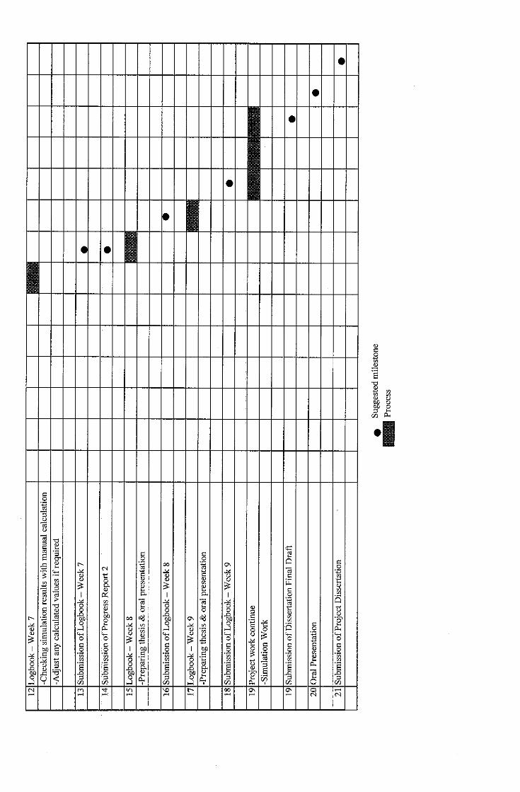
APPENDIX 1
Suggested Milestones

Su
gg
este
dM
iles
ton
efo
rth
eF
irst
Sem
este
ro
f2S
emes
ter
Fin
alY
ear
Pro
ject
No
.D
eta
il/W
eek
12
34
56
7S
91
01
11
21
31
4
1S
elec
tion
of
Pro
ject
Top
ic
-Pro
po
seto
pic
-To
pic
assi
gned
toth
est
uden
t
2L
ogbo
ok-
Wee
k3
-Stu
dyon
proc
ess
requ
irem
ent
for
GD
CP
lant
-Stu
dyon
mec
hani
cal
requ
irem
entf
orG
DC
Pla
nt
3S
ubm
issi
ono
fLog
book
-W
eek
3•
4P
reli
min
ary
Res
earc
hW
ork
-In
tro
du
cti
on
-Ob
ject
ive
-Lis
to
fre
fere
nces/l
itera
ture
-Pro
ject
pla
nn
ing
5S
ubm
issi
ono
fP
reli
min
ary
Rep
ort
•
6L
ogbo
ok—
Wee
k4
-Lit
erat
ure
rev
iew
onlo
adfl
owst
udy
for
the
syst
em
-Lit
erat
ure
revi
ewon
pow
erfl
owfo
rth
esy
stem
7S
ubm
issi
ono
fL
ogbo
ok-
Wee
k4
•
8L
ogbo
ok-
Wee
k5
-Ele
ctri
cal
load
anal
ysis
base
don
the
real
syst
em
-Cal
cula
tem
axim
um
dem
and
and
peak
load
9S
ubm
issi
ono
fLog
book
-W
eek
5•

10
Log
book
-W
eek
6
-Des
ign
sing
lelin
edi
agra
m
-Cal
cula
tesi
zing
for
all
maj
oreq
uipm
ents
11
Sub
mis
sion
ofL
ogbo
ok-
Wee
k6
•
12
Lo
gb
oo
k-
Wee
k7
-Cal
cula
tesi
zing
for
all
cabl
es
13
Sub
mis
sion
ofL
ogbo
ok-
Wee
k7
•
14
Sub
mis
sion
ofP
rogr
ess
Rep
ort
•
15
Log
book
-W
eek
8
-Lit
era
ture
rev
iew
on
sho
rtcir
cu
it
16
Sub
mis
sion
of
Log
book
-W
eek
8•
17
Log
book
-W
eek
9
-Cal
cula
tesh
ort
circ
uit
for
each
bubs
bar
man
ually
18
Su
bm
issi
on
ofL
ogbo
ok-
Wee
k9
•
19
Lo
gb
oo
k-
Wee
k10
-Cal
cula
tesh
ort
circ
uit
for
each
bubs
bar
man
uall
y
-Sta
rtdo
ing
soft
war
esi
mul
atio
n
20
Sub
mis
sion
ofL
ogbo
ok-
Wee
k10
•
8O
ral
Pre
sent
atio
n&
Inte
rim
Rep
ortP
repa
rati
on
9S
ubm
issi
ono
fInt
erim
Rep
ort
•S
ug
ges
ted
mil
esto
ne
Pro
cess

Su
gg
este
dM
iles
ton
efo
rth
eS
eco
nd
Sem
este
ro
f2
Sem
este
rF
inal
Yea
rP
roje
ct
No
.D
eta
il/W
eek
12
34
56
78
91
01
11
21
31
4
1L
ogbo
ok—
Wee
k2
-Co
nti
nu
eso
ftw
are
sim
ula
tio
n
2S
ub
mis
sio
no
fL
og
bo
ok
-W
eek
2•
3L
ogbo
ok-
Wee
k3
-Co
nti
nu
eso
ftw
are
sim
ula
tio
n
-Des
ign
SL
Dfo
rde
tail
des
ign
4S
ub
mis
sio
no
fLog
book
-W
eek
3•
5S
ub
mis
sio
no
fP
rogr
ess
Rep
ort
1•
6L
og
bo
ok
-W
eek
4
-Co
nti
nu
eso
ftw
are
sim
ula
tio
n
-Com
pari
ngsi
mul
atio
nre
sult
ofba
sic
and
desi
gn
7S
ubm
issi
ono
fL
ogbo
ok-
Wee
k4
•
8L
og
bo
ok
-W
eek
5
-Ch
eck
ing
sim
ulat
ion
resu
lts
with
man
ual
calc
ulat
ion
9S
ubm
issi
ono
fL
ogbo
ok-
Wee
k5
•
10
Log
book
-W
eek
6
-Che
ckin
gsi
mul
atio
nre
sult
sw
ithm
anua
lca
lcul
atio
n
-Ad
just
any
calc
ulat
edva
lues
ifre
quir
ed
11S
ub
mis
sio
no
fL
ogbo
ok-
Wee
k6
•
12
Log
book
-W
eek
7
-Che
ckin
gsi
mul
atio
nre
sult
sw
ith
man
ual
calc
ulat
ion
-Adj
usta
nyca
lcul
ated
valu
esif
requ
ired
13
Sub
mis
sion
ofL
ogbo
ok—
Wee
k7
•
14
Sub
mis
sion
of
Pro
gres
sR
epor
t2
•
15
Log
book
-W
eek
8
-Pre
pari
ngth
esis
&or
alpr
esen
tati
on
16
Sub
mis
sion
ofL
ogbo
ok-
Wee
k8
•
17
Log
book
-W
eek
9
-Pre
pari
ngth
esis
&or
alpr
esen
tati
on
18
Sub
mis
sion
ofL
ogbo
ok—
Wee
k9
•
19
Pro
ject
wo
rkco
ntin
ue
-Sim
ula
tio
nW
ork
19
Su
bm
issi
on
of
Dis
sert
ati
on
Fin
al
Dra
ft•
20
Ora
lP
rese
nta
tio
n•
21
Sub
mis
sion
of
Pro
ject
Dis
sert
atio
n•
Sug
gest
edm
iles
tone
Pro
cess

APPENDIX 2
Major Process Flow Diagram

211V-O30|
P-05CPA/B
VL SERVICESIHD.
'2003
PUTRAJAYA HOLDINGSfUTFMJMA HnOIMPI KM. Mi.nul PDI1UHIUH "TMiMJt KRSCKUTIMMWRAJM*
seuwmwu. qsjw.pel : oi-skrh
w*. oi-tzEzus/x
GAS ^"*cooling K^3PUTRHJAIA ^•'^
OS DiSTRKT COOLING (PUTRAJAYA) C3M. BHD.pctwas tvin raws"wi urn* cirr ffMiirsowkwla tww.wt.ns,*.Tel. W. s Ol-Jtai 7579f«. H»i 01-JX6I 7600.
&mll_t i
cgi level j i. u_t«r ?fiS^* remans Twin roios•£_ kuju lww cm com*.
Tel. *. , CO-ZOSI Urn
fi* Iheto'cW Mt
Un.Wfjsd %Mcia>l«j<nl
fi» IWOnf tB»
:
Tib *•>•) u Gsrti^il.Cabactvi «l cm* ill driaiMI at i>lc 0,1,f%Hl l«niu »t I. be»rt Hkieomk, Hit
tnoHHne.
PUffiAJAYA
PBEONCT5 .
DBJftlCT CO&JNG PLANT PROJECT
Qr«*»J-,.l. ,i f
OVERALL PROCESSFLOW DIAGRAM
-WS; c-fin f
Oni,*. i • 5 .*
" HA? i
oa. 09.M
pjps-BRa-oi-oooi
F" ^'W*™ COC ^ojEct^flFC-rV^

APPENDIX 3
Electrical Load Analysis for Basic and Detail
Engineering Design

LO
AD
LIS
TF
OR
3.3
kV
SW
ITC
HG
EA
R
EQ
UIP
.
TA
GN
O.
DE
SC
RIP
TIO
N
QU
AN
TIT
YC
ON
DIT
ION
o u 2a.
°a
ao
3:
MO
TO
RS
PE
CIF
ICA
TIO
NC
ON
TIN
UO
US
INT
ER
MIT
TE
NT
ST
AN
D-B
Y
LU % w U
LU
o V)
•o C
UJ % t/i
3 s
1c 2 W
°O
Q£
ZO
2=
MO
TO
R
RA
TIN
G
<kW
)E
FF
I.P
.F
MO
TO
R
LO
AD
(kW
)
TO
TA
L
LO
AD
(kW
)k
VA
Rk
VA
TO
TA
L
LO
AD
(kW
)k
VA
Rk
VA
TO
TA
L
LO
AD
(kW
)k
VA
Rk
VA
RE
SW
RK
P-0
20
1A
-FC
OO
LIN
GW
ATE
RPU
MP
FOR
DFC
].,
••
65
1A
IM1
60
0,8
00
0.0
31
0.8
30
13
7.8
68
7.4
46
2.0
82
8.2
13
7.5
92
.41
65
.60
.00
.00
.0L
oad
IsC
on
firm
ed
P-0
10
1A
-0C
UST
OM
ER
TR
AN
SF
ER
ING
PUM
P(S
EC
ON
DA
RY
PUM
P)4
31
AIM
25
00
.80
00
.93
80
.64
62
13
.26
39
.74
03
.17
56
.12
13
,21
34
.42
52
.00
.00
.00
.0L
oad
IsC
on
flrm
od
Ph
ase
1G
RA
ND
TO
TA
L1
00
00
82
13
27
.18
65
,11
58
4.3
35
0.7
22
8.8
41
7.7
0.0
0.0
0.0
EQ
UIP
.
TA
GN
O.
DE
SC
RIP
TIO
N
QU
AN
TIT
YC
ON
DIT
ION
o 2cl
o<
3
2
MO
TO
RS
PE
CIF
ICA
TIO
NC
ON
TIN
UO
US
INT
ER
MIT
TE
NT
ST
AN
D-B
Y
w o w n c
LU
CD
v>
LU I (fl
£
C
c 01
c
O0
2O
25
MO
TO
R
RA
TIN
G
(kW
)E
FF
I.P
.F
MO
TO
R
LO
AD
(KW
)
TO
TA
L
LO
AD
(kW
)k
VA
Rk
VA
TO
TA
L
LO
AD
(kW
)
kV
AR
kV
A
TO
TA
L
LO
AD
(*W
)
kV
AR
kV
AR
EM
AR
K
P-0
20
1G
-NC
OO
LIN
GW
AT
ER
PU
MP
FO
RD
FC
33
2e
eIM
16
00
.60
00
.93
10
.83
01
37
.61
09
9.9
73
9.1
13
25
.20
.00
.00
.00
.00
.00
.0L
ou
dIt
Co
nfU
mo
d
P-0
10
1E
-HC
UST
OM
ER
TR
AN
SFE
RIN
GPU
MP
(SE
CO
ND
AR
YPU
MP)
21
14
BIM
25
00
.BO
00
.03
60
.64
62
13
.26
02
.98
37
.61
00
8.1
0.0
0.0
0.0
0.0
0.0
0.0
Lo
ad
liC
nn
flrm
od
Ph
ase
2to
Ph
ase
4G
RA
ND
TO
TA
L0
54
31
20
19
52
.S1
27
6.7
23
33
.30
.00
.00
.00
.00
.00
.0
GDCP
SPr
elim
Load
UsL
_rev
O_b
acku
pLO
AD
IJST
3.3K
Y

EQ
UIP
.
TA
GN
O.
DE
SC
RIP
TIO
N
Kit
dm
s^
mw
^m
^^
^M
^^
^^
WS
CT
-02
01
A-L
CO
OL
ING
TO
WE
R(F
AN
SX
2N
OS
).'(
P-0
30
1A
.BM
AK
E-U
PW
AT
ER
PU
MP
FO
RC
OO
LIN
GW
AT
ER
P-0
30
2A
.BM
AK
E-U
PW
ATE
RPU
MP
FOR
CH
ILLE
DW
ATE
R'
•'l'
\
P-0
10
3A
.BS
IDE
ST
RE
AM
FIL
TE
RP
UM
P
DF
C-0
10
1A
-FD
IRE
CT
FIR
ED
CH
ILL
ER
/No
.1A
bsor
bent
pum
p'
IN
o.2
Ab
sorb
ent
pu
mp
/R
eWg
eran
lp
um
p
/P
urg
ep
um
p
'.'
//
bu
rner
blo
wer
P-01
02A
-FC
HIL
LE
DW
AT
ER
PUM
PFO
RD
FC(P
RIM
AR
Y)
mm
m?
mm
mm
P-0
40
1A
.BD
IES
EL
TR
AN
SF
ER
PU
MP
P-0
40
2A
.BO
ILS
UP
PL
YP
UM
PF
OR
DF
C
P-O
40
3A
.BO
ILS
UP
PL
YP
UM
PF
OR
GE
NE
RA
TO
R
ti^
jbm
^M
^^
m^
^^
Bui
ldin
gse
rvic
es
MO
V
UP
Ssy
slem
s
CC
SD
islr
ibu
tio
nB
oard
Rem
ote
I/O
Cab
inet
Ph
ase
1G
RA
ND
TO
TA
L
CDCP
SPr
elim
Load
Lis
Lje
vO-b
icku
p
IM.
Q-T
Y
12
24
87
LO
AD
LIS
TF
OR
41
5V
SW
ITC
HG
EA
R
CO
ND
ITIO
N
10
24
75
12
O O 50
.
ao
2
IM IM IM IM IM IM IM IM IM IM IM IM IM IM
MO
TO
RS
PE
CIF
ICA
TIO
N
MO
TO
R
RA
TIN
G
(kW
)
30
0,5
5
3.7
7.5
3.7
0.4
0:7
5
15
00
0.5
5
0.7
5
0.7
5
15
0
0.3
80
27
3.5
EF
FI.
P.F
0.8
00
0,9
29
0.8
69
0.8
00
o.e
oe
0.7
88
0.8
00
0.7
48
0.8
71
0.8
00
0.8
57
0.8
09
0.B
00
0.8
82
0.7
89
0.8
00
0.8
57
0.8
09
0.8
00
0.7
23
0.6
64
0.6
00
0.7
48
0.6
71
0.8
00
0.9
15
0.7
95
0.8
00
0.9
36
0.6
61
0.8
00
0.7
48
0,6
71
0.8
00
0,7
48
0.6
71
o.e
oo
0.7
48
0.8
71
1.0
00
1.0
00
1.0
00
0.8
00
0.7
23
0.6
04
1.0
00
1.0
00
1.0
00
1.0
00
1.0
00
1.0
00
1.0
00
1.0
00
1.0
00
MO
TO
RL
OA
D
(kW
)
25
,92
9.7
1
0.5
9
3.4
5
6.8
0
3.4
5
0.4
4
0.6
0
13
.11
78
.92
0.5
9
0.8
0
0.8
0
15
0.0
0
0.3
3
80
.00
27
.00
3.5
0
CO
NT
INU
OU
S
TO
TA
L
LO
AD
(kW
)
25
0.2
9.7
0.6
3.5
34
.0
17
.3
2.2
4.0
65
.6
36
4.6
0.6
0.6
0.8
15
0.0
8.0
80
.0
27
.0
7.0
10
54
.9
WA
R
14
7.6
7.6
0.7
2.8
26
.5
12
.6
2.5
4.4
50
.0
22
7.2
0.7
0.9
0.9
0.0
0.0
0.0
0.0
0.0
40
3.0
kV
A
29
8.3
12
.4
0.9
4.3
43
.1
21
.3
3.3
6.0
82
.5
44
8.7
0.9
1.2
1.2
15
0.0
12
.0
60
.0
27
.0
7.0
11
96
.0
INT
ER
MIT
TE
NT
TO
TA
L
LO
AD
(kW
)
51
.8
0.7
0.0
0.0
8.8
3.5
0.4
0,8
13
.1
76
.9
0.6
0.8
0.8
0,0
0,0
0.0
0.0
0.0
16
5.3
kV
AR
29
.5
7.8
0.0
0.0
5.3
2.5
0.5
0.9
10
.0
45
.4
0.7
0.9
0.9
0.0
0,0
0.0
0.0
0.0
10
4.2
kV
A
59
.7
12
.4
0.0
0.0
B.f
l
4.3
0.7
1.2
16
.5
89
.3
0.9
1.2
1.2
0.0
0.0
0.0
0.0
0.0
19
5.9
ST
AN
D-B
l'
TO
TA
L
LO
AD
(kW
)k
VA
Rk
VA
RE
MA
RK
m.
Lo
ad11
Co
nfi
rmed
Lo
ad
IsC
on
firm
ed
mm
®L
oad
IsC
on
firm
ed
Lo
adIs
Co
nfi
rmed
Lo
ad
IkC
on
firm
ed
Lo
adIs
Co
nfl
rmo
d
Lo
ad
llC
on
fVm
od
Lo
ad
IsC
on
firm
ed
Lo
ad
liC
on
flrm
od
Lo
ad
ItC
'.onf
lrm
ed
Lo
9d
IsC
on
flrm
od
Loa
dIst
jonf
lrmed
Lo
adIs
Co
nfl
rmed
LOAD
IJ5T
05V
(A)

LO
AD
LIS
TF
OR
41
5V
SW
ITC
HG
EA
R
CDCP
5Pr
elim
Load
UsL
-rer
CLb
acV
upLO
ADIJ
ST41
6V

B)
MA
XIM
UM
LO
AP
NO
DE
SC
RIP
TIO
Nk
Wk
VA
rk
VA
1T
OT
AL
CO
NT
INU
OU
SL
OA
D3
27
9.8
6"
21
41
.75
39
17
.22
23
0%
OF
TO
TA
LIN
TE
RM
ITT
EN
TL
OA
D1
05
.21
68
12
5.2
9.1
LA
RG
ES
TIN
TE
RM
ITT
EN
TL
OA
D2
13
.22
13
4.3
82
53
.f\3
MA
XIM
UM
I,O
AIJ
(R
EF
ER
NO
TE
1)
34
93
.08
22
76
.13
41
69
.12
PF
.AK
LO
AD
_Q_
NO
DE
SC
RIP
TIO
Nk
Wk
VA
rk
VA
1M
AX
IMU
ML
OA
D3
49
3.0
82
27
6.1
34
16
92
2
21
0%
OF
TO
TA
LS
TA
ND
BY
LO
AD
0.0
00
.00
0.0
0
3L
AR
GE
ST
ST
AN
DB
YL
OA
D"
....
0.0
00
.00
0.0
0
PE
AK
LO
AD
(RE
FF
.RN
OT
E2
)3
49
3.0
82
27
6.1
34
16
9.1
2
LV
DB
A)
SU
MM
AR
Y
NO
DE
SC
RIP
TIO
NC
on
lin
uo
uj
Inte
rmit
ten
tS
tan
db
yk
Wk
VA
rk
VA
kW
kV
Ar
kV
Ak
Wk
VA
rk
VA
1T
OT
AL
LY
BO
AR
D2
30
6.9
51
26
1.3
12
62
9.2
51
65
.28
10
4.2
21
95
.39
0.0
00
,00
0
B)
MA
XIM
UM
LO
AR
NO
DE
SC
RIP
TIO
Nk
Wk
VA
fk
VA
1T
OT
AL
CO
NT
INU
OU
SL
OA
D2
30
6,9
51
26
1.3
12
62
9.2
32
30
%O
FT
OT
AL
INT
ER
MIT
TE
NT
LO
AD
49
.58
31
.26
58
.61
iL
AR
GE
ST
INT
ER
MIT
TE
NT
LO
AD
76
.92
45
.44
S9
J-J
MA
XIM
UM
LO
AD
(R
EF
ER
NO
TE
1)
23
83
.88
13
04
.75
27
18
.34
QP
EA
KL
OA
D
NO
DE
SC
RIP
TIO
Nk
Wk
VA
rk
VA
IM
AX
IMU
ML
OA
D2
38
3.8
81
30
6.7
52
71
8.5
*2
10
%O
FT
OT
AL
ST
AN
DB
YL
OA
D.
..._
-.
0.0
0_
0.0
01
1.0
0
3L
AR
GE
ST
ST
AN
DB
YL
OA
D0
.00
0.0
0O
.Od
PE
AK
LO
AD
(RE
FE
RN
OT
E2
)2
38
3.8
81
30
6.7
32
71
8.3
4
TO
TA
LL
OA
DT
OC
AT
ER
Max
imu
mL
oad
3.3
KV
+M
ax
imu
mL
oad
41
5V
58
76
.96
kW
68
87
,78
kV
A
NO
TE
S:
1.M
AX
IMU
ML
OA
D
3.P
F.A
KL
OA
D
GDCP
IiPr
elim
Load
Lis
U-e
vO-b
ecku
p
TO
TA
LC
ON
TIN
UO
US
LO
AD
*(3
0%
OF
INT
ER
MIT
TE
NT
LO
AD
OR
LA
RG
ES
TIN
TE
RM
ITT
EN
TL
OA
DW
IIIC
ItE
VE
RIS
CR
EA
TE
R)
MA
XIM
UM
LO
AD
+(1
0%
OF
ST
AN
D8
VL
OA
DO
RL
AR
GE
ST
STA
ND
BY
LO
AD
WH
ICH
EV
ER
ISC
RE
AT
ER
)
LOAD
SUMM
ARY
(«ll)

PJP5 District Cooling Plant Project - 3.3 kV Tran:
Equip. NO Serial No Equipment Name
ConUououi Load (WA> Rerun t
Sll Phase
P-0101 A lo E Secondary ChinedWaier Pumps
<F1» Speed)628
P-0102 A to C
EC-0121
P-0231 A to M
Secondly Cndled Water Pumps
(VARIABLE FREQUENCY DRIVE)
Electrical Chiller
Coolin? Water Pump for DFC
453
:ondib'on for Transformer Capacity Selection.i.oat
270
^352
1 For General Oration,
t.1 Status for Transformer Operation- Individual operation condition, each transformer to s—:ply t.^°-Air cooled fan (AF) for transformer NOT lo be operated during
.2 11/3.3kV Transformer Load Estimation (AN Operation):Minimum required transformer capacity WITHOUT forced air cc~-ForPhase 1only = 2750kVA (with 3.3k) kVA ,AM, ._-ForAJIPhases(1,2.3&4> = 5100 kVA (mil). J f******1***1^™** ^ffPritT "inft Wrr]
453
767
192
959
3.081
314
302
616
154
770
Total
1.571
990
1.023
1.963
5,547
1.387
6.333
8.933
(kVA)
Uncorrected kVA
PF before correction a q a;
The above AN rating is selected with PF correction capacitor bP*** Continuous Load (kvA)Remark i
2 For Urgent or Maintenance Operation fas Back-no nppr.tm, ".1 Status for Transformer Operation
- During either one (1) transformer isfail orunder maintenance,electricity toboth busbars ofthe 3.3 kV switchgear (with 16501 —
-The 5100 kVA (AN rating) transformer is still capable of supply
2 Transformer LoadEstimation forSpare Load of 25%-For Phase 1only = 3800 kVA AF (with PF «r- For Phase 1and Future = 6325 WA AF (withPFco
CONCLUSION '
Proposed Selection for 11/3.3 kV Transformer rating (AN/AF) sh;Dynlt. ±5% in 2.5 step. Z% =6.0% on 5.1 MVA, where AF ratin<
Hoia
AF rating of 7140 kVA >maximum toaad of 6993 kVA (uncorrectiatAF rating can supply total load WITHOUT powe'r factor correct!
enam* •11-3.3kVTransform*. Setectfo* Rev , edited bvZul.xls
503
3015
Total
5,058 PF after correction » 0.95
1,265
6,323
Rev. 1

PJP5 District Cooling Plant Project -11 / 0.433 kV Transfon
Equip. No Serial Ne Equipment N«H
Phaw
t 2 1
311 SI 2 Total
)FC-0I31 A la N
Tnot
USFcl
Oicd-Ficd Alxarptiori CN*« 2 3 5 3 3
;r-02ci A lo M Cooling Tdwm k* OFC-OtOI 3 3 6 3 3
—'-0J21 Cooling Wji« Pump for EC t 0 1 0 0
'•013t A to H OiJVefl Water Pump k» DFC 2 3 5 3 3
'0121 CWftefl W«« Pump fw EC 1 0 1 0 a (—
'-1 i ! i •\ ID 3 Ma*e up #mer Pump Id* CjweG Water
(t lUndhyl
2 0 2 0 a
i'1121 A to C Make up wafer pump lor a>o*r>g rraler
(t lUndbf)2 0 2 1 0
1
'-oi o* aid e GrculMina; Pump toi Swi S»eam Pfler
{1 Itandby)
2 0 2 0 0 a
:u-o«'o Chcmtca* doling unrt lor Owiec Water 1 0 1 0 0 <r
:u-a*zi Otemcal ooimg unn tor CooW>g Water I 0 1 0 0 q
IIMUS CftemtcaJ doling unr lor Cookni) Water 1 0 1 0 0 a
'•0501 A-S Oi!!u9p*y p-jrre lor T-05C1 2 a 2 a 0 o—
'-osaz A-B Oi supply puma tor T-0S01 0 0 0 2 0
'-0503 A-B Oil Hippty pump lor T-0503 2 0 2 Q 0 o'—
:ire Ftghtzng 1,, 0 0 0 0 a—
Win
CoM Water 1 0 1 0 0 0;
Suiting Savkxx 1 0 1 0 0 0;—
ACMVEqu*™*
1 0 1 0 0 a
Eusa
1 • 1 0 i
Condition for Transformer Capacity Selection"VS*
1 For General Operation
1.1 SUtu* for Transformer Operation r"
- Individual operation condition, each transformer losupply theetecfricity for each bu- **" cooledfan(AF) fortransformer NOT to be operatedduring this status n
1.2 11/ 0.433kVTransforrnerLoad Estimation (AN Operation): —Minimum Required Transformer Capacity WITHOUT Forced Air Cooled fanoperatioi• For Phase 1 onfy =: 1500 kVA (with 415Vpower'factorcorrection
- For Phase 1.2.314 * 1600 kVA x 2 (estmaied fromuncorrected KVA) —
The aOoveANrating is selected with PF correction capacitor banks to improve the
2 For Urgentor MaintenanceOperation (as Back-upoperation,
L1 Status for Transformer Operation• Ouring eitherone (1)transformer is tailor undermaintenance, the alternative transt '
to supply the electricity to both Ousoar in 415V svrichoear / MCC- The 1600kVA (AN rating)transformer ts stHt capable of supplyingthe total load
L2 Transformer Load Estimation for Spare Load of 25%- For Phase 1 only =1770 kVA & (with PF correctioncapac- ForPhase 1* Future =1770kVAx2 ** (with PF correction capa<
CONCLUSION
Proposed Selection for 11 / 0.433 kVTransformer rating (AN/AF) shalDyrt 11,* 5% in"2.5 STEP, ZV. = G.Q %on 1S00 kVA. where AF rating i:
Haw
AF rating of22*0WA>m*OTUTi loud of21*9kVA (uncorrected), tnerekxeone(1
Ver. 1

APPENDIX 4
Group Derating Factor

JNSIALLATION ON CAR. F ;annrpc
ENO
TJMETHOD tTLADDER
TRAY
TOUCHING
SPACED
| TREfOH. FORMATION
X CORE CABLES IN TREFOIL FORMAT.™
NGEUENTABLES
NjJMKR OF INSTALLATION IN TREFOILCABLE
LADDERS(LAYERS)
CLEARANCE = 2dDCTA^fTOMWALL'220mm
g£ CABLES - SPACED
:ment£S W**OF ^ARArCE =CABtED(A«ETERd
^ | ^n^KAIL;>20rnrn(LAYERS)
NUMBER OF CABLES PER LADDER
1.00 Q.98 0.S6 0.93 0.92
'•00 0.95 0.93 0.90 0.89
3><45 1.00 I 0.94 0.92 0.89 0.88
1-00 0.93 0.90 0.87 0.86
CABLES - TOUCHING
NT NUMBER OF s«OE BY SJOE WITHOUT aEARANCE«^ (AND TOUCH.NG WALL ""**(UYERS)
NUMBER Of CABLES PER LADDER
0.95 0.84 0-80 0.75 2&0.95 0.80 0.76 0.71 0.69
3, A & 5 0.95 0.78 0-74 070 0.68
0.95 0.76 0.72 0.68 0.66
kL-alA.
|a •Q fti
ssmaszm.
U 11
- SINGLE CORE- TREFOIL- SPACING
Mn-LD-ifVTPr-cp
u u
- MUITI CORE- SPACING
MTI-LD-.y-qp
ssmsse^jiU 11
- MULU CORE- SINGLE LAYER- TOUCHING
Mn-LD-.Wrr
I. t
IIi

APPENDIX 5
Cables Reference Tables

IftUKAlUfi MfiUSVSI
3LE 1: SINGLE-CORE 600/10OOV (CVWAZV)XLPE/PVC/SWA(AL)/PVCSTRANDED COPPER CONDUCTOR
Jen&fication : Natural
BLE 2: TWO-CORE 600/1000V (CVWAZV)XLPE/PVC/SWA/PVC
STRANDED COPPER CONDUCTOR
ien&atron ; Red arxj K>*

unuKmun mnuwsi IEC 60502-2
bie 1 3.6/6(Max. 7.2) KV THREE-CORE CABLESCopper conductor
Sfwpeof
strand
Approx.outer
da.
Thidc.
of
XLPE
irtsuiafjon
PVC separatorShaath
Thrdc Approxouter
kcSa.
{mm}
Cia.
of
jarYarizecsteel
*wre
Thick,
of
PVC
outer-
sbeath
Approx.overaJI
cSa.
Approx.-rei.
weight
electrical charadertstia?
Ojrrert rating Cooduclof resistance Capacitance
Reactance Shorta150Hi
{mm)
4.7
5.97.0
8.1
{mm) (mm)
TT1.2
1.2
1.3
1.4
1.4
1.5
1.5
{mm) (mm) (mm) (kfjAm)
lr. air
at 40°C
(A)
in the
groundat2S°C
"Tib-140
170
200
O.C.
at20°C
(fl/km)
50Hz
at90°C
(11/km) (rf/Vm) (Q/km)
dtaA
current
(or
Isec
(kA)
Ciraiar
compact
9.7
11.4
12.8
14.3
16.0
18.4
20.6
23.3
263
25
2.5
2.5
25
2S
2,5
2.5
2-5
2.5
26
2.83.0
3.2»nt»fiGBicrt : i»d. ys4ow & &o«
1.6
1.7
1.8
2.0£1
31.6
34.2
37.0
39.6
43.7
47.3
50.6
53.8
57.7
63.5
69.3
76.3
83.9
20
2.0
20
2.5
2.5
15
25
2.5
2.5
2.5
3.153.15
22
23
23
2.5
26
2.7
28
29
3.0
32
3.5
3.8
3.15 4.0
40.5
43.0
46.0
50.0
54.0
58.0
61.5
65.0
69.0
75.083.0
90.5
98.5
2.8303,3303,8404,870
5.9107.0208.0809.210
10.71013,09016.41019.88023,820
105
13?
195
245
300
340
385
440
515585
665
745 i 650
245
290
330
365
1.15
0.727
0.524
0.387
0.268
0.193
0.1530.124
415 0.0991
475530
0.07540.0601
0.0470
1.47
0.927
0.668
0.494
0.342
0.2470.196
0.160
0.128
0.0988
;o.osoo0.0643
0.0366 0.0522
0.21
0.24
0.28
0.31
0.350.40
0.43
0.47
0.520.56
0.57
J1600.62
0.117
0.109
0.105
0.100
0.0949
0.0914
0.0885
0.08600.0837
0.0817
0.0805
0.07900.0779
2.41
3.725.18
7.36
10.2
13.8
17.4
21.8
26.8
34.7
43.4
57.7
72.1
ble 2 6/10 (Max. 12) KV THREE-CORE CABLES
irlicaiion ; rod. j-eoow 4 Dh>e
16,38,7/15 (Max. 17.5) KV THREE-CORE CABLESper conductor Trie*.
Of
XLPE
insulation
PVC separationsheath
Shapeof
strand
Approx.outer
(mm) (mm)
5.9 4.5
7.0 4.58.1 4.5
9.7 4.5
Circular 11.4 45
12.8 4.5
:ompacl 14.3 4.5
16.0 4.5
18.4 4.5
20.6 I 4 5| 23.3 ; .* fi
I 26 2 : •1 :>
Thick.
1.4
1.4
1.5
1.5
1 6
1.7
1.7
1 8
1 9
2 0
Approx.outer
ola.
(mm)
43.3
46.1
48.7
52.6
56.4
59.7
62.9
66 7
72-i i
Dia.
of
galvanizedsteel
wire
2.5
2.5
2.5
2.5
2.5
2.5
2.5
3.15
3.15
3.15
3 15
3 15
Thick,
of
PVC
outer-
sheath
(mm)
2.6
2.7
2.8
2.9
3.0
3.1
3.2
3.4
36
3.7
40
42
Approx.overall
dia.
54.0
57.0
59.5
63.5
67.5
71.0
74.5
80.0
86.0
91.0
97.5
104 5
Approx,net
weight
(kcykm)
4,790
5,4206,0807,160
8,350
9,46010.640
13,090
15.550
17.950;
21.300-25 HO
Ourrerf rating
In air
at 4frC
(A)
M0
170
200
250
305
350
395
,150520"590
665
In the
ground3t2S°C
(A)
140
170
200
245
290
330
370
J 10
"47?530
^90
Electrical characteristics
CorirJudof resistance
D.C.
ai20°C
(0./km)
0.727
0.524
0.387
0.268
0.193
0.153
0.124
0_0_9910.0754
0.0601
0 04 70
o o.3f.f;
50Hz
at90°C
(n/km)
0.927
0.663
0.494
0.342
0.247
0.196
0 159
0.126
0.09830 0791
0 0536,
Capacitance
li£/tm)
0.16
0.18
0.20
0.22
0.25
0.27
0.29
0.31
0.35
0 38
0-52
Reactance Shortat50Hz
(n/km)
0.131
0.124
0.118
0.112
0.107
0.103
0.0994
0.0962
0.0924
0 0896
0 08680OHJ?
droit
currer*
(or
1 sec
(kA)
3.72
5.18
7.36
10.2
13.8
17.4
21.8
26.8
34.7
43 4
57 7
72 1
•GC
c

APPENDIX 6
Short Circuit Ratings

<Vp da*- &eqcU*
srtcircuit ratingsPPER CONDUCTORS
FIGURE 2 m
'alues of fault current given in the graph Figure 2ased on the cable being fully loaded at the staiti short circuit (conductor temperature 90°C) andilconductor temperature of 250°C. and itshould
be ensured that the accessories assoctated with thecable are also capable of operation at these values oifault current and temperature.
o-i 0-2 0-3 0-4 0-5 0-6 0-8 1"0 2-0
OURATION OF SHORT CIRCUIT IN SECONDS
Y!>e IsmrV IrtA.*fOjf>rn? COn'VCiOrs (ttis;cjdo! IhC ccvnp,eswi type) 'SnofICCCVTimcna-X i-VCf-V" L'OC «w,'.c si'.tc™
Djrj fcv stitntlsdakjtrvniijn) cofdunln/s a'c a.ailatifc on icguesr
3-0

APPENDIX 7
Fuse Link Type CMF

Fuse link type CMF Appe<*Ac-*. 5-
Ken 2000 30C0
motor starting current (A)
WOO 2000
motor storting current ( A ,
mole* staring current IA)
3UO0
3000
10. Choice of fuse links
Choice of rated voltage U^:
The rated voltage of the .use linksmust beequal to,or higher than the operating linevoltage. By choosing (uselink rated voltageconsiderably higher than the linevoltage,the maximum arc voltage mustnot exceedthe insulation level of the network.
Choice of rated current 1^:
The minimum permissible currentratingofthe fuse link for motor protection may bedetermined from the selection charts I, IIand III.The three different charts are for
run-up times of6,15 and 60 secondsrespectively. Eachchartcontains differentcharacteristics, dependingon the number ofstarts per hour. Ofthisspecific numberofstarts per hour, the first two areinimmediate succession; the rest being evenlyspacedinthe 1 hourperiod. The number ofstarts per hour indicatesthe timeintervalbetween seperate starts. For example,4 starts in 15 minutes are represented by 16starts per hour.
On the horizontal axis of the selection chart,the motor starting current is given, andalong the vertical axis thecurrent rating ofthe fuse link is found.
Selection procedure:
- Select the charts which are appropriatefor the run-up time of the motor. .
- select the starting current along thehorizontal axis,
- depending on the number of starts perhour, select the correct characteristic(2.4,8, 16.32),
- read of the correct rating of the fuse linkon the vertical axis.
Example: A B
Starting current of the motor
Run-up time
Number ol starts per hour
Chart number
Rated current ol fuse.1 link
850A
6 sec.
2
1
250A
250A
15 sec.
16
2
160A
ABB Kraft

xise link type CMF
—?M r r— ] [,.......
•*<' —
--v-x-^-*
I ~^T v _L\ ' .
?V * k \
>T1 \
) : — '.-.
H±^
\ N\* \ s \ \\
' .3 V.-i-4-ft y. \ ' \I w — --V *--v* V L... _ •
Tj 7ft -^—s-^-iv—
:? S3 t 0 160X0 so as
••si \ \-\l_^__. 1 •
c tt*
—=S=-Jr^r-\V-A \ \ * ' 0
ai
n,-Vvv-i-* —- - A--V-JA^
\v \ \
\ 1V ^ )*V" 2 J 1
Current /
> > t
Strom in A ——^
i j * • i t?
Kraft
/\z_
/?
T // + ••'
\ • ^<<
1 > •>*p*i •**-'' **•'-'-'-
~£ ^/ ^-"" T' ^^
^^^^
1
S 13 20 SO IM
Pro^Mtlivr curitr* kA |rms)
7. Pre-arcinn times
The characteristics are equal for all rated
voltages and are recorded from coldcondition.
In the uncertain interrupting zone the curvesare dotted.
8. Current limitation
CMF fuse links are current limiting. A large
short circuit current will therefore not reach
its full value. The diagram shows the relationbetween the prospective short circuit currentand the peak value og the cut off current.
9. Overvoltages
In orderlo be currentlimiting, the fuse links'must generate an arc voltage exceeding theinstantaneous value of the operatingvoltage. Theovervoltage generated by theCMF fuse link is below the maximum
permissible value ace to IEC282-1.CMFfuse links can safely be used if thesystem line voltage is 50-100% of the rated(use link voltage.
]Q

Fuse link type CMF
11. Replacement of melted fuse links
The fuse link cannot be regenerated.
According to IEC. Publication 282-1, all 3fuse links should be replaced, even ifonry 1or 2 of the fuse links in the threephase
12. The K-factor
According to the IEC 644, the K-factor is afactor {less than unity) d.eftning an overloadcharacteristic to which the fuse link may be
repeatedly subjected under specified motorstarting conditions without deterioration. Theoverload characteristic is obtained by
13. Data and dimensions CMF
system have operated. Exceptions areallowed when it can be verified that the fuse
link(s) have not experienced anyovercurrent
multiplyingthe currenton the prearcingcharacteristic (melting time characteristics)by K.The Value of K given in the data tableis chosen at 10 seconds melting time, and isvalid for melting times between 5 and 60
seconds.
UN •n e D K* '1 '3 Ro PNMinimum Maximum
IM
. kV A mm mm -KA A mohm Watt
Pre-arc
Aas
Interruption
A*s
•Q? \ 292 65 0,75 50' 275 3,25 49 1,4-104 (17-104 )\
292 65 0,7 50 -400 1,94 75 3,8 '104 L50-104 J
3,6 200 292 87 0,7 50 500 1,42 75 7,6'104 71 -104
^250^ 292 87 0,6 50 760 1.03 90 14-104 v?:10**?315 292 87 0,6 50 900 0,85 122 21*10"* 180-104
63 442 65 0,75 50 175 8,63 45 0,48 • 104 6,5-104
100 442 65 0,75 50 275 4,93 67 1,40* 104 18 • 104
7,2160 442 65 0,7 50 400 2,96 119 3,8 *104- 54-104
200 442 87 0,7 50 500 2,15 118 7,6-104 75-104
250 442 •87* 0,6 50 800 1,56 142 14- 104 120* 104
315 442 87 0,6 50 950 1,30 193 21 • 104 220-104
63 442 65 0,75 50 190 13,3 77 0,48 • 104 11 -104
12100 442 87 0,75 50 275 6,72 103 1,4- 104 20 "104
160 442 87 0.7 50 480 4,04 155 3,8-10" 70 • 104
200 442 87 0,7 50 653 2.89 173 9,3- 104 91 • 104
c CMF 3 s
*) The K-lactor is relened to the
average value of current.
ABB Kraft
Legends:
e = see figureD = see figure
K = K-factor ace. to IEC 644
Ij = max. short circuit current testedl3 - minimum breaking currentRq = resistance at room temperaturePN = power loss at rated current
Nil sna'Si-i* C:

APPENDIX 8
Proposed Cable Sizes

SHINRYO(M)SDNBHDPROJECT: PUTRAJAYA PRECINCT 5POWER CABLES SCHEDULE SUMMARY -41.S\>
"Group Derating Factor = 0.73
iV SWGR.xls

SHINRY0(M)SDN8HDPROJECT: PUTRAJAYA PRECINCT 5POWER CABLE SCHEDULE SUMMARY -3 3kV Swit
Cabfe Schedule Rev l.xis
3.3 kv swot

SHINRYO (M)SON BHDPROJECT : PUTRAJAYA PRECINCT 5POWER CABLE SCHEDULE SUMMARY - 415V VSD Los
From To
Transformer A
Transformer B
Transformer C
-#B*-AVFDB
VEQ.C
VFDA
VFDB
VFDC
Variable Frequ"Variable Frequf
P-0102A
P-0102B
Variable FrequSecondary Chille
P-0102C^Secondary Chille-,^Secondary Chute
Cable Schedule Rev t.xls
No of
Core type Or Cable
JC/S/P (Cu)jusrp (Cu)JC/S/P (Cu)
JCS/R(CuTX/S/P(Cu).
JO§/P.(Cu)
Proposed Cable
Size(sq.mm)
500
500
500
400:
'WQ.-&:
400.:^
Ampacity ofcable at 40
deg.C
870
870
870
"n&Tsd^s?^SZOTKSJSilS©
Remarks
%^P-J
3.3 KVSWGR (415V VSD Load)

APPENDIX 9
Crystal Report-Short Circuit Simulation for Basic
Engineering Design

Pro
ject:
Basi
c_
f=n
gin
eeri
ng
_5
r
DA
PP
ER
Fa
ult
Co
ntr
ibu
tio
nC
om
ple
teR
ep
ort
Da
te:
2D
ecem
ber
20
04
Tim
e:
4:0
2:5
4P
M
Co
mp
reh
en
siv
eS
ho
rtC
ircu
itS
tud
yS
ett
ing
s
Th
ree
Ph
ase
Fau
ltY
es
Sin
gle
Lin
eto
Gro
un
dY
es
Lin
eto
Lin
eF
au
ltN
o
Lin
eto
Lin
eto
Gro
un
dN
o
Mo
tor
Co
ntr
ibu
tio
nY
es
Tra
nsf
orm
er
Tap
No
Xfo
rmer
Ph
ase
Sh
ift
Yes
-In
itia
lS
ym
metr
ical
Am
ps-
Bu
sN
am
e
llk
VS
'bo
ard
ll/3
.3a
11
/3.3
b
11
/41
5a
11
/41
5b
11
a
3.3
kV
Bu
s
3.3
a
3.3
b
3.3
kV
Fu
ture
3.3
kV
Ph
ase
1
41
5V
Bu
sl
ll/4
15
a2
41
5V
Ph
ase
1
41
5V
Ph
asel
InC
ab
le
Ou
Cab
le
InC
ab
le
Ou
Cab
le
InC
ab
le
InC
ab
le
Ou
Cab
le
InIn
dM
a
inIn
dM
a
inC
ab
le
InIn
dM
a
inIn
dM
tr
3P
hase
17
,31
3
1,0
61
29
6
15
,95
8
17
,61
3
13
,19
1
2,3
84
2,0
50
43
,78
2
33
,96
8
4,9
73
4,9
73
SL
G 0 0 0 0
17
,56
0
14
,62
0
1,5
85
1,3
62
41
,13
3
34
,97
9
3,1
15
3,1
15
LL
G 0 0 0 0
Fau
lted
Bu
s
Bu
sV
olt
ag
es
Bran
ch
Cu
rren
ts
Ph
ase
or
Seq
uen
ce
Fau
ltC
urr
en
tC
alc
ula
tio
n
Asy
mF
au
ltC
urr
en
tat
Tim
e
AH
Bu
ses
Fir
st
Bu
sF
rom
Fau
lt
Fir
stB
ran
ch
Fro
mF
au
lt
Rep
ort
ph
ase
quan
titi
es
Init
ial
Sym
met
rica
lR
MS
(wit
h1/
2C
ycle
Asy
m)
0.5
0
-Asy
mm
etr
ical
Am
ps-
—In
itS
ym
Neu
tral
Am
ps-
LL 0 0 0
3P
hase
27
,64
1
1,6
94
47
3
25
,47
8
SL
G 0 0 0
28
,44
62
8,9
40
21
,30
52
4,0
95
3,8
51
2,6
12
3,3
11
2,2
46
52
,18
84
7,9
84
40
,49
04
0,8
05
5,9
28
3,6
33
5,9
28
3,6
33
LL
G 0 0 0
LL 0 0 0
SL
G
17
,56
0
41
,13
3
LL
G

—in
itsy
mN
eu
icra
iA
mp
s—
Bu
sN
am
e3
Ph
ase
SL
GL
LG
LL
3P
ha
se
SL
GL
LG
LL
SL
GL
LG
41
5V
Bu
s2
00
00
00
00
ll/4
15
b2
InC
ab
le0
00
00
00
0
41
5V
Ph
ase
2In
Ind
Mtr
2,2
56
1,4
80
00
2,6
37
1,7
09
00
41
5V
Ph
ase2
InIn
dM
tr2
,25
61
,48
00
02
,63
71
,70
90
0
HkV
No
deB
us4
17
,26
00
00
27
,29
50
00
11
/41
5a
InC
ab
le1
6,9
66
00
02
6,8
29
00
0
11
/0.4
15
Tx
lAIn
Xfo
rmer2
29
60
00
46
80
00
HkV
No
deB
us7
00
00
00
00
11
/41
5b
Ou
Cab
le
11
/0.4
15
Tx
lBO
uX
form
er2
HkV
No
deB
us9
17
,27
10
00
27
,45
60
00
ll/3
.3a
InC
ab
le1
6,2
10
00
02
5,7
70
00
0
1l/
3.3
kV
Tx
AIn
Xfo
rmer2
1,0
61
00
01
,68
70
00
3.3
kV
No
de4
17
,63
51
7,5
90
00
28
,59
42
9,1
44
00
3.3
aIn
Cab
le4
,43
12
,94
60
07
,18
44
,88
10
0
H/3
.3k
VT
xA
InX
form
er2
13
,21
81
4,6
52
00
21
,43
22
4,2
76
00
17
,59
1
HkV
No
deB
us3
17
,35
40
00
27
,86
00
00
11
aIn
Cab
le1
,35
70
00
2,1
78
00
0
TN
B1
InU
til.
16
,00
00
00
25
,68
60
00
HkV
No
deB
us2
00
00
00
00
ll/3
.3b
Ou
Cab
le
11
/3.3
kV
Tx
BO
uX
form
er2
3.3
kV
No
de5
00
00
00
00
3.3
bO
uC
ab
le
11
/3.3
kV
Tx
BO
uX
form
er2

Bu
sN
am
e
41
5V
No
de
Bu
s4
ll/4
15
a2
11
/0.4
15
Tx
lA
41
5N
od
eB
us5
11
/41
5b
2
11
/0.4
15
Tx
lB
InC
ab
le
InX
form
er2
InC
ab
le
Ou
Xfo
rmer2
-In
itia
lS
ym
metr
ical
Am
ps-
3P
hase
SL
GL
LG
LL
51
,36
04
9,5
90
00
9,4
27
6,0
68
00
42
,04
24
3,5
87
00
-Asy
mm
etr
icalA
mp
s—
—In
itS
ym
Neu
tral
Am
ps-
3P
hase
SL
GL
LG
LL
SL
G
82
,92
28
2,0
43
00
15
,22
01
0,0
39
00
67
,87
87
2,1
12
00
49
,59
0
LL
G

APPENDIX 10
Crystal Report-Short Circuit Simulation for Detail
Engineering Design

rro
jeci:
ueta
n_
cn
gin
een
ng
_o
r
DA
PP
ER
Fa
ult
Co
ntr
ibu
tio
nC
om
ple
teR
ep
ort
Date
:2
Decem
ber
20
04
Tim
e:
4:1
0:3
5P
M
Co
mp
reh
en
siv
eS
ho
rtC
ircu
itS
tud
yS
ett
ing
s
Th
ree
Ph
ase
Fau
ltY
es
Sin
gle
Lin
eto
Gro
un
dY
es
Lin
eto
Lin
eF
au
ltN
o
Lin
eto
Lin
eto
Gro
un
dN
o
Mo
tor
Co
ntr
ibu
tio
nY
es
Tra
nsf
orm
er
Tap
Yes
Xfo
rmer
Ph
ase
Sh
ift
Yes
-In
itia
lS
ym
metr
ical
Am
ps-
Bu
sN
am
e
Hk
VS
'bo
ard
B
11
/3.3
M
ll/4
15
bl
PI-
1
llkV
S'b
oa
rd
A
ll/3
.3al
ll/4
15
al
11
a
PI-
1
3.3
kV
Bu
s2
11
/3.3
b2
Tx
VF
DB
PI-
2
P-0
10
1D
-E
P-0
23
1C
-E
Ou
Cab
le
Ou
Cab
le
InP
i
InC
ab
le
InC
ab
le
InC
ab
le
InP
i
Ou
Cab
le
InX
form
er2
InP
i
InIn
dM
tr
InIn
dM
tr
3P
hase
15
.81
8
15
,81
8
15
,81
9
1,4
50
32
0
15
,48
7 0
20,041
590
17,258
836
593
SL
G 0
16,548
325
15,016
460
326
LL
G 0
Fau
lted
Bu
s
Bu
sV
olt
ag
es
Bran
ch
Cu
rren
ts
Ph
ase
or
Seq
uen
ce
Fau
ltC
urren
tC
alc
ula
tio
n
Asy
mF
ault
Cu
rren
tat
Tim
e
All
Bu
ses
Fir
st
Bu
sF
rom
Fau
lt
Fir
st
Bra
nch
Fro
mF
au
lt
Rep
ort
phas
equ
anti
ties
Init
ial
Sym
met
rica
lR
MS
(wit
h1/
2C
ycl
eA
sym
)
0.5
0
-Asy
mm
etr
ical
Am
ps-
—In
itS
ym
Neu
tral
Am
ps-
LL 0
3P
hase
15
,81
8
15
,81
8
15
,81
9
1,4
50
32
0
15
,48
7 0
SL
G 0
24,559
22,990
723
451
21,149
20,860
1,024
639
727
453
LL
G 0
LL 0
SL
GL
LG
16,548

wa.
E<
30)
z
E>>
(3
C3
0
o
EE
inoSO
OssoOS
oOSr-
oooooooo
oooooooo
O 00oo CN
r~-"
M r> m o on m r>m cn ro o oOs rn so m so
c-1so"
O CN
<n VI
•* so r-iM 00 >O ^f C
oooooooo
oooooooo
Os SO fi so o o oin r-i o ->3- oo m ^oin 00 N in \D N t
so' of —<"
co r>
lOWM«MlOhtsosoo** — roososcNmootN'tf,ooror>
g 43 fc 43 43 43
•S (£ T3 13 -O 73 13
c c e c c c c .=
3Gfl <
£y Qf!
£fO
Kro r-. i-
c-ro o
< X
(N olO OU
PL, W Oh Oh Oh Oh
OOOOOOOOOOO
O OOOOOOOOOOO
r>in
r-f
(Nr^m^©0'-'**r--mrNy3•—' ^- so ^t m n « (NOsr- cn 'Jj- O m
o * ~ -* -
molooommoor^co^soosr-so — oooomtN m in^T c» ro so —-^ -hos" so" ri t-T f\f
ooooooooooo
ooooooooooo
<N \o mW ro —i
oo in mtS *tf
i© m -^- co ^©
o
c-4 m os oo r-- r- r-im ^r o m so -*too in Os ro r-
tN r- os soCN N M
U cu
43 43
243
243 43 43 43 43
243
IT3
cT3
CT3
e c13 T3
C13
c c
cccccccacpic:
CN —u
I "*• /<f
=3 < $5pa •3 _: o o
> in CN ^9 9
o
Ui H D Uh
Tf — Oh u u u
z < <kO rn
o o
<:<<:< m
o om mo o
Oh Oh Oh 0-1 Oh Oh Oh
O O O O
O O O O
oCs^r
\o oo inOSlO
oo ^•*
inm
mso
r4 so
CN in fN —'
o o o o
o o o o
in oOs
oo so OS
in
oo
SOO
OSoCs
oOOs
Ol-*
so —'
<u
43 43
243 43
2
nt-a T3 t3
3
o n £ a c3
O
IX ffl
M Q3 rN
J3
(Jo-l m
oa
>if) 5 ro
o o
3
oi
Uo
o
•* i— Oh U U u Oh
rs

Bu
sN
am
e
P-0
12
1A
P-0
13
1D
-E
P-0
22
1
P-0
50
1B
P-0
50
2A
-B
P-0
50
3B
P-1
11
1B
HkV
No
deB
usl
ll/3
.3al
Tx
ll/3
.3k
VA
3.3
kV
No
del
ll/3
.3a2
Tx
11
/3.3
kV
A
HkV
No
deB
us2
ll/3
.3b
l
Tx
ll/3
.3k
VB
3.3
kV
No
de2
ll/3
.3b
2
Tx
ll/3
.3k
VB
HkV
No
deB
us3
11
a
TN
B
HkV
No
deB
us4
ll/4
15
al
Tx
11
/0.4
15
A
Hk
VN
od
eB
usS
11
/41
5M
InIn
dM
tr
InIn
dM
tr
InIn
dM
tr
InIn
dM
tr
InIn
dM
tr
InIn
dM
tr
Ou
Ind
Mtr
InC
ab
le
InX
form
er2
InC
ab
le
InX
form
er2
Ou
Cab
le
Ou
Xfo
rmer2
Ou
Cab
le
Ou
Xfo
rmer2
InC
ab
le
InU
til.
InC
ab
le
InX
form
er2
Ou
Cab
le
-In
itia
lS
ym
metr
ical
Am
ps-
3P
hase
58
0
1,1
61
91
8
22
43 7
15
,64
2
15
,35
8
1,4
51
20
,12
9
6,8
46
13
,35
6 0
16,292
1,764
16,000
15,610
15,521
320 0
SL
G
35
2
70
4
55
7
13
26 4
16
,63
5
3,7
72
12
,89
8 0
LL
G 0 0 0 0 0 0
LL 0 0 0 0 0 0
3P
hase
72
2
1,4
44
1,1
43
27
54
15
,64
2
15
,35
8
1,4
51
24
,69
4
8,3
98
16
,38
4 0
16,292
1,764
16,000
15,610
15,521
320 0
-Asy
mm
etr
ical
Am
ps-
SL
G
44
6
89
2
70
6
17
33 5
23
,20
4
5,2
61
17,9
91
0
LL
G 0 0 0 0 0 0
LL 0 0 0 0 0 0
—In
itS
ym
Neu
tral
Am
ps-
SL
GL
LG
16
,63
5

Bu
sN
am
e
Tx
11
/0.4
15
B
41
5V
No
de
Bu
sl
11
/41
5a2
Tx
11
/0.4
15
A
41
5V
No
de
Bu
s2
11
/41
5b
2
Tx
11
/0.4
15
B
41
5V
No
de
Bu
s3
Tx
VF
DA
P-0
10
2A
41
5V
No
de
Bu
s4
Tx
VF
DB
P-0
10
2B
-C
Ou
Xfo
rmer2
InC
ab
le
InX
form
er2
Ou
Cab
le
Ou
Xfo
rmer2
InX
form
er2
InIn
dM
tr
InX
form
er2
InIn
dM
tr
-In
itia
lS
ym
metr
ical
Am
ps-
3P
hase
45
,43
0
10
,51
7
34
,92
8 0
14
,14
2
10
,39
6
3,7
56
17
,88
4
10
,38
8
7,5
11
SL
G
41
,63
2
6,4
25
35
,21
6 0
12
,98
4
10
,69
1
2,2
99
14
,89
3
10
,73
0
4,1
70
LL
GL
L
-Asy
mm
etr
ical
Am
ps
3P
hase
64
,98
4
15
,04
4
49
,96
2 0
SL
G
63
,74
7
9,8
38
53
,92
2 0
22
,68
52
1,4
24
16
,67
61
7,6
39
6,0
24
3,7
93
27
,98
52
4,3
25
16
,25
61
7,5
25
11
,75
46
,81
1
LL
GL
L
—In
itS
ym
Neu
tral
Am
ps-
SL
GL
LG
41
,63
2
12
,98
4
14
,89
3

APPENDIX 11
Crystal Report-Load Flow Simulation for Basic
Engineering Design

Date
:2
Decem
ber
20
04
Tim
e:
3:5
8:0
4P
M
Lo
ad
Flo
wS
tud
yS
ett
ing
s
Inclu
de
So
urc
eIm
ped
an
ce
So
luti
on
Meth
od
Lo
ad
Sp
ecif
icati
on
Gen
erati
on
Accele
rati
on
Facto
r
Sw
ing
Gen
era
tors
So
urce
In/O
ut
Serv
ice
TN
B1
In
Bu
ses
Bu
sN
am
eIn
/Ou
tS
erv
ice
Hk
VN
od
eB
us2
In
Hk
VN
od
eB
us3
In
Hk
VN
od
eB
us4
In
Hk
VN
od
eB
us7
In
Hk
VN
od
eB
usS
In
Hk
VN
od
eB
us9
In
llk
VS
'bo
ard
In
Pro
ject:
Basi
cJE
ng
ineeri
ng
_L
c
Lo
ad
Flo
wS
um
mary
Rep
ort
Vp
u
1.0
0
Yes
Ex
act
(Ite
rati
ve)
Co
nn
ecte
dL
oad
1.0
0
An
gle
0.0
0
Desi
gn
Vo
lts
11
.00
0
11
.00
0
11
.00
0
11
.00
0
11
.00
0
11
.00
0
11
.00
0
kW
4,4
51
.0
Lo
ad
Accele
rati
on
Facto
r
Bu
sV
olt
ag
eD
rop
%
Bra
nch
Vo
ltag
eD
rop
%
kv
ar
VD
%
3,4
59
.61
.21
LF
Vo
lts
An
gle
Deg
ree
PU
Vo
lts
10
.86
6-0
.82
0.9
9
10
.86
7-0
.82
0.9
9
10
.86
6-0
.82
0.9
9
10
.86
6-0
.82
0.9
9
00
.00
0.0
0
10
.86
6-0
.82
0.9
9
10
.86
6 1
-0.8
20
.99
1.0
0
5.0
0
3.0
0
Uti
lity
Imp
ed
an
ce
0.0
1+j
0.3
3
%V
D
1.2
2
1.2
1
1.2
2
1.2
2
10
0.0
0
1.2
2
1.2
1

Bu
sN
am
eIn
/Ou
tS
erv
ice
3.3
kV
Bu
sl
In
3.3
kV
Bu
s2
In
3.3
kV
No
de3
In
3.3
kV
No
de4
In
3.3
kV
No
de5
In
33
kV
No
de
Bu
sl
In
33
kV
No
de
Bu
s2
In
33
kV
No
de
Bu
s3
In
41
5N
od
eB
us5
In
41
5V
Bu
sl
In
41
5V
Bu
s2
In
41
5V
No
de
Bu
s4
In
BU
S-3
3k
VIn
Cab
les
Desi
gn
Vo
lts
3.3
00
3.3
00
3.3
00
3.3
00
3.3
00
33
.00
0
33
.00
0
33
.00
0
41
5
41
5
41
5
41
5
33
.00
0
LF
Vo
lts
3.2
18
3.2
11 0
3.2
19
3.2
12 0 0 0
40
5
40
2
40
2
40
5 0
An
gle
Deg
ree
-31
.78
-31
.93
0.0
0
-31
.78
-31
.94
0.0
0
0.0
0
0.0
0
-31
.70
-31
.63
-31
.63
-31
.70
0.0
0
PU
Vo
lts
0.9
8
0.9
7
0.0
0
0.9
8
0.9
7
0.0
0
0.0
0
0.0
0
0.9
8
0.9
7
0.9
7
0.9
8
0.0
0
%V
D
2.4
7
2.6
8
10
0.0
0
2.4
6
2.6
7
10
0.0
0
10
0.0
0
10
0.0
0
2.3
6
3.1
7
3.1
7
2.3
6
10
0.0
0
Fro
mB
us
To
Bu
s
Co
mp
on
en
tN
am
e
In/O
ut
Servic
e
%V
DkW
Lo
ss
kva
r
Lo
ss
kV
A
Lo
ss
LF
Am
ps
Ra
tin
g%
PF
Hk
VN
od
eB
us3
llk
VS
'bo
ard
11
aIn
0.0
14
,45
1.0
0.3
3,4
59
.6
0.3
5,6
37
.4
0.4
29
9.5
0.0
0.7
9
llk
VS
'bo
ard
Hk
VN
od
eB
us2
11
/3.3
bIn
0.0
01
,86
2.8
0.0
1,4
54
.3
0.0
2,3
63
.3
0.1
12
5.6
0.0
0.7
9
llk
VS
'bo
ard
Hk
VN
od
eB
us4
11
/41
5a
In0
.00
49
3.1
0.0
38
0.8
0.0
62
3.0
0.0
33
.1
0.0
0.7
9
llk
VS
'bo
ard
11
/41
5b
In0
.00
49
3.1
38
0.8
62
3.0
33
.10
.79

Fro
mB
us
To
Bu
s
Co
mp
on
en
tN
am
e
In/O
ut
Servic
e
%V
DkW
Lo
ss
kva
r
Lo
ss
kV
A
Lo
ss
LF
Am
ps
Ra
tin
g%
PF
Hk
VN
od
eB
us7
0.0
0.0
0.0
0.0
llk
VS
'bo
ard
Hk
VN
od
eB
us9
11
/3.3
aIn
0.0
01
,60
1.6
0.0
1,2
43
.4
0.0
2,0
27
.6
0.0
10
7.7
0.0
0.7
9
3.3
kV
No
de4
3.3
kV
Bu
sl
3.3
kV
No
de5
3.3
kV
Bu
s2
3.3
a
3.3
b
In0
.01
In
0.0
1
1,6
01
.6
0.2
1,8
62
.8
0.2
1,2
01
.2
0.1
1,3
97
.1
0.2
2,0
02
.0
0.2
2,3
28
.4
0.3
35
9.1
0.0
41
8.6
0.0
0.8
0
0.8
0
41
5N
od
eB
us5
41
5V
Bu
s2
ll/4
15
b2
In0
.81
49
3.1
4.5
36
8.9
2.5
61
5.8
5.2
87
7.4
0.0
0.8
0
41
5V
No
de
Bu
s4
41
5V
Bu
sl
ll/4
15
a2
In0
.81
49
3.1
4.5
36
8.9
2.5
61
5.8
5.2
87
7.4
0.0
0.8
0
2-W
ind
ing
Tra
nsf
orm
ers
Fro
mB
us
To
Bu
s
Co
mp
on
en
tN
am
e
In/O
ut
Serv
ice
%V
Dk
W
Lo
ss
kv
ar
Lo
ss
kV
A
Lo
ss
LF
Am
ps
Rat
ing
%P
F
1lk
VN
od
eB
us
3.3
kV
No
de5
11
/3.3
kV
Tx
BIn
1.4
51
,86
2.8
0.0
1,4
54
.3
57
.2
2,3
63
.2
57
.2
12
6.0
39
.9
0.7
9
llk
VN
od
eB
us
41
5V
No
de
Bu
s
11
/0.4
15
Tx
lAIn
1.1
54
93
.1
0.0
38
0.8
11
.9
62
3.0
11
.9
33
.0
31
.5
0.7
9
llk
VN
od
eB
us
41
5N
od
eB
us5
11
/0.4
15
Tx
lBIn
1.1
54
93
.1
0.0
38
0.8
11
.9
62
3.0
11
.9
33
.0
31
.5
0.7
9
llk
VN
od
eB
us
3.3
kV
No
de4
H/3
.3k
VT
xA
In1
.25
1,6
01
.6
0.0
1,2
43
.3
42
.1
2,0
27
.6
42
.1
10
8.0
34
.2
0.7
9

APPENDIX 12
Crystal Report-Load Flow Simulation for Detail
Engineering Design

Da
te:
2D
ecem
ber
20
04
Tim
e:
4:0
7:5
4P
M
Lo
ad
Flo
wS
tud
yS
ett
ing
s
Inclu
de
So
urc
eIm
ped
an
ce
So
luti
on
Meth
od
Lo
ad
Sp
ecif
icati
on
Gen
erati
on
Accele
rati
on
Facto
r
Sw
ing
Gen
era
tors
So
urce
In/O
ut
Serv
ice
TN
BIn
Bu
ses
Bu
sN
am
eIn
/Ou
tS
erv
ice
1lk
VN
od
eB
usl
In
Hk
VN
od
eB
us2
In
Hk
VN
od
eB
us3
In
Hk
VN
od
eB
us4
In
llk
VN
od
eB
us5
In
1lk
VS
'bo
ard
AIn
1lk
VS
'bo
ard
BIn
Vp
u
1.0
0
Pro
ject:
Det
ail_
En
gin
eeri
ng
_L
c
Lo
ad
Flo
wS
um
ma
ryR
ep
ort
Yes
Ex
act
(Ite
rati
ve)
Ist
Lev
elD
eman
dor
En
erg
yF
acto
r
1.0
0
Lo
ad
Accele
rati
on
Facto
r
Bu
sV
olt
ag
eD
rop
%
Bra
nch
Vo
ltag
eD
rop
%
An
gle
kW
kv
ar
VD
%
0.0
06
,10
2.3
1,6
81
.02
.06
Desi
gn
Vo
lts
LF
Vo
lts
An
gle
Deg
ree
PU
Vo
lts
10
.76
30
.26
0.9
8
10
.76
30
.26
0.9
8
10
.77
30
.28
0.9
8
10
.76
40
.26
0.9
8
10
.76
40
.26
0.9
8
10
.76
40
.26
0.9
8
10
.76
40
.26
0.9
8
1
11
.00
0
11
.00
0
11
.00
0
11
.00
0
11.000
11.000
11.000
1.0
0
5.0
0
3.0
0
Uti
lity
Imp
ed
an
ce
0.3
3+J
0.0
1
%V
D
2.16
2.15
2.06
2.14
2.15
2.14
2.14

Bu
sN
am
eIn
/Ou
tS
erv
ice
3.3
kV
Bu
sl
In
3.3
kV
Bu
s2In
3.3
kV
No
del
In
3.3
kV
No
de2
In
41
5V
Bu
sl
In
41
5V
Bu
s2
In
41
5V
No
de
Bu
sl
In
41
5V
No
de
Bu
s2
In
41
5V
No
de
Bu
s3
In
41
5V
No
de
Bu
s4
Cab
les
Fro
mB
us
To
Bu
s
In
Co
mp
on
en
tN
am
e
Hk
VN
od
eB
us3
11
a
llk
VS
'bo
ard
A
1lk
VS
'bo
ard
A
llk
VN
od
eB
usl
llk
VS
'bo
ard
A
Hk
VN
od
eB
us4
llk
VS
'bo
ard
B
Hk
VN
od
eB
us2
llk
VS
'bo
ard
B
Hk
VN
od
eB
us5
ll/3
.3al
ll/4
15
al
11
/3.3
M
11
/41
5M
Desi
gn
Vo
lts
In/O
ut
Serv
ice
In In In In In
3.3
00
3.3
00
3.3
00
3.3
00
41
5
41
5
41
5
41
5
41
5
41
5
%V
D
0.0
8
0.0
1
0.0
0
0.0
1
0.0
0
LF
Vo
lts
kW
Lo
ss
6,1
02
.3
4.4
2,7
18
.5
0.3
52
4.8
0.0
1,9
73
.1
0.2
88
1.5
0.0
3.3
40
3.3
51
3.3
41
3.3
52
42
1
41
9
42
3
42
2
42
9
42
0
An
gle
Deg
ree
kv
ar
Lo
ss
1,6
81
.0
3.5
88
2.7
0.3
77
.9
0.0
60
4.5
0.1
11
2.4
0.0
-3.6
8
-1.1
4
-1.6
7
-1.1
4
-0.9
7
-1.8
3
-0.9
2
-1.7
2
-3.7
1
-5.2
7
kV
A
Lo
ss
6,3
29
.6
5.6
2,8
58
.3
0.4
53
0.6
0.0
2,0
63
.6
0.2
58
.6
0.0
PU
Vo
lts
1.0
1
1.0
2
1.0
1
1.0
2
1.0
1
1.0
1
1.0
2
1.0
2
1.0
3
1.0
1
LF
Am
ps
Rat
ing
%
33
9.2
0.0
15
3.3
0.0
28
.5
0.0
11
0.7
0.0
47
.7
0.0
%V
D
-1.2
1
-1.5
5
-1.2
4
-1.5
6
-1.4
1
-1.0
5
-1.8
1
-1.7
1
-3.3
1
-1.1
4
PF
0.9
6
0.9
5
0.9
9
0.9
6
0.9
9

Fro
mB
us
To
Bu
s
Co
mp
on
en
tN
am
e
In/O
ut
Serv
ice
%V
Dk
W
Lo
ss
kv
ar
Lo
ss
kV
A
Lo
ss
LF
Am
ps
Rat
ing
%
PF
3.3
kV
No
del
3.3
kV
Bu
sl
ll/3
.3a2
In0
.03
2,7
18
.1
0.6
78
2.1
0.6
2,8
28
.4
0.8
48
8.8
0.0
0.9
6
3.3
kV
No
de2
3.3
kV
Bu
s2
ll/3
.3b
2In
0.0
21
,97
2.8
0.3
55
2.0
0.3
2,0
48
.6
0.4
35
2.9
0.0
0.9
6
41
5V
No
de
Bu
sl
41
5V
Bu
sl
ll/4
15
a2
In0
.39
52
4.8
2.0
66
.8
0.8
52
9.0
2.1
72
2.9
0.0
0.9
9
41
5V
No
deB
us2
41
5V
Bu
s2
11
/41
5b
2In
0.6
58
81
.4
5.5
81
.5
2.2
88
5.2
5.9
1,2
10
.8
0.0
1.0
0
2-W
ind
ing
Tra
nsf
orm
ers
Fro
mB
us
To
Bu
s
Co
mp
on
en
tN
am
e
In/O
ut
Serv
ice
%V
Dk
W
Lo
ss
kv
ar
Lo
ss
kV
A
Lo
ss
LF
Am
ps
Rat
ing
%P
F
llk
VN
od
eB
us
3.3
kV
No
del
Tx
11
/3.3
kV
AIn
-3.3
92
,71
8.2
0.1
88
2.4
10
0.4
2,8
57
.9
10
0.4
15
3.0
57
.3
0.9
5
1lk
VN
od
eB
us
3.3
kV
No
de2
Tx
ll/3
.3k
VB
In-3
.72
1,9
72
.9
0.1
60
4.3
52
.3
2,0
63
.4
52
.3
11
1.0
41
.3
0.9
6
11k
VN
od
eB
us
41
5V
No
de
Bu
s
Tx
11
/0.4
15
AIn
-3.9
55
24
.8
0.0
77
.9
11
.0
53
0.6
11
.0
28
.0
33
.9
0.9
9
llk
VN
od
eB
us
41
5V
No
de
Bu
s
Tx
l1
/0.4
15
BIn
-3.8
58
81
.4
0.0
11
2.4
30
.9
88
8.6
30
.9
48
.0
56
.8
0.9
9
3.3
kV
Bu
sl
41
5V
No
de
Bu
s
Tx
VF
DA
In-2
.10
28
3.8
0.0
18
2.2
13
.9
33
7.2
13
.9
58
.0
83
.3
0.8
4
3.3
kV
Bu
s2
41
5V
No
de
Bu
s
Tx
VF
DB
In0
.41
56
7.6
0.1
39
4.7
57
.9
69
1.3
57
.9
11
9.0
17
0.2
0.8
2

PiIm
ped
an
ces
Fro
mB
us
To
Bu
s
Co
mp
on
en
tN
ame
llk
VS
'bo
ard
AP
I-1
llk
VS
'bo
ard
B
3.3
kV
Bu
s2
3.3
kV
Bu
sl
41
5V
Bu
s2
41
5V
Bu
sl
PI-
2
PI-
3
%V
D
0.0
0
0.0
0
0.0
0
kW
Lo
ss
2,8
54
.5
0.0
0.0
0.0
0.0
0.0
kv
ar
Lo
ss
71
6.9
0.0
0.0
0.0
0.0
0.0
kV
A
Lo
ss
2,9
43
.2
0.0
0.0
0.0
0.0
0.0
LF
Am
ps
Rati
ng
%
15
7.9
0.6
0.0
0.0
0.0
0.0
PF
0.9
7
0.0
0
0.0
0

APPENDIX 13
Simulation Diagrams-Branch and Bus Fault Currents
for Basic Engineering Design

llk
VS
'bo
ard
11
/41
5a
-I1
Isc
3P
29
6A
4-
Isc
3P1
69
66
A
ll/0.
415T
xIA
g
-t
Isc3
PP
ri2
96
A4
Isc
3P
42
04
2A
4Is
cS
LG
43
58
7A
41
5V
Ph
ase
l
Isc
3P
49
73
A
Isc
SL
G3
11
5A
']••Is
c3
P1
06
1A
4-Is
c3
P1
62
10
A
Isc3
PP
ri
10
61
A
Isc3
P1
32
18
A
Isc
SL
G1
46
52
A
11
/41
5a2
-TIs
c3
P9
42
7A
1XIs
cS
LG
60
68
A4
Isc
3P
33
96
8A
4Is
cS
LG
34
97
9A
41
5V
Ph
asel
isc
3P
49
73
A
Isc
SL
G3
11
5A
TN
B1
lkV
(Ph
ase
1-P
hase
2)
Isc
3P
16
00
0A
1"Is
c3
P1
35
7A
4-Is
c3
P1
59
58
A
Il/
3.3
kV
Tx
A
|Is
Isc
3P44
31A
i.3.
3a4-
Isc
SLG
2946
A4
-Is
c3
P1
31
91
A4-
Isc
SL
G1
46
20
A
®!
3.3
kV
Ph
asel
Isc
3P
20
50
A
Isc
SL
G1
36
2A
11
/3.3
kV
Tx
B
03
.3k
VF
utu
re
Isc
3P
23
84
A
Isc
SL
G1
58
5A
J11
/415b
U/0
.4l5
Tx
lB
0'
41
5V
Ph
ase
2
Isc
3P
22
56
A
Isc
SL
G1
48
0A
J®
41
5V
Ph
ase2
Isc
3P
22
56
A
Isc
SL
G1
48
0A

43
78
2A
mp
s3P
41
13
3A
mp
sS
LG
1731
3A
mps
3Pll
kV
S'b
oard 11
/415
aJ
11
/0.4
15
Tx
lA
04
15
VP
hasel
ll/4
15
a2
1761
3A
mp
s3P
17
56
0A
mp
sS
LG
TN
B1
lkV
(Ph
ase
1-P
has
e2}
(i)
H/3.3
kVTx
A
03
.3k
VP
hase
l
!1
/3.3
b
11/3
,3kV
TxB
fgs,
3.3
b
03
.3k
VF
utu
re
li/4
15
b
S)
11/0
.415
Txl
B
ill
/41
Sb
2
04
15
VP
hase
2

APPENDIX 14
Simulation Diagrams-Branch and Bus Fault Currents
for Detail Engineering Design

-as
-a*
-GUI
•H31
—a——--© g)
-®s
HSISS
.-©3
-®IE| -®m
^i||
3 I-H---
!S-
9g!
•*£«
5 2r=
ia
-®Ies
--©gas
BJ3

! ra-
-«t§S^ ^\_i-
-HB-- HB'
s"-@—-
-Eh—
V
H®i
-^
S J,
~©>E
9—®2
—^—-©»
43*
-©?
^
-®|
HSS
-©=
3
-©5
H^
— -— -Si
H3i

APPENDIX 15
Simulation Diagrams-Load Flow Study without
Power Factor Correction for Basic Engineering
Design

LF
VD
%1
.21
%
llk
VS
'bo
ard
11
/41
5a
]1
/0.4
15
Tx
lA
44
93
.1k
W
43
80
.8k
VA
R
PctV
D1
.1%
41
5V
Bu
sl
LF
VD
%3
.17
%^
^
4-4
93
.1k
W4
38
0.8
kV
AR
PctV
D0
.0%
LF
33
A3.
3kV
Bus
l
16
01
.6k
W
12
43
.4k
VA
R
PctV
D0
.0%
LF
10
8A
16
01
.6k
W
12
43
.3k
VA
R,
PctV
D1
.2%
'
LF
VD
%2
.47
%
Il/4
15
a2
4-
49
3.1
kW
4-3
68
.9k
VA
RP
ctV
D0
.8%
LF
87
7A
fkf
41
5V
Ph
asel
61
0.7
0k
VA
04
45
1.0
kW
34
59
.6W
AR
44
51
.0k
W
34
59
.6k
VA
RP
ctV
D0
.0%
LF
30
0A
H/3
.3k
VT
xA
16
01
.6k
W
12
01
.2k
VA
R
PctV
D0
.0%
LF
35
9A
3.3
kV
Ph
ase
l
20
01
.80
kV
A
4-
18
62
.8k
W
4-1
45
4.3
kV
AR
PctV
D0
.0%
LF
12
6A
H/3
3k
VT
xB
.
4-1
86
2.8
kW
4-1
39
7.1
kV
AR
PctV
D0
.0%
LF
41
9A
03
.3k
VF
utu
re
23
28
.17
kV
A
18
62
.8k
W
14
54
.3k
VA
RP
ctV
D1
.5%
3.3
kV
Bu
s2
LF
VD
%2
.68
%
j11
/415
b$_
-J-
493.
1kW
43
80
.8k
VA
RP
ctV
D0
.0%
LF
33
A
ll/0
.4I5
Tx
lB
44
93
.1k
W4
38
0.8
kV
AR
PctV
D1
.1%
H/4
15
b2
44
93
.1k
W
J-
36
8.9
kV
AR
PctV
D0
.8%
LF
87
7A
04
15
VP
hasel
61
0.7
0W
A
LF
VD
%3
.17
%

11
/0.4
15
Tx
lA
33.1
0Pr
iAm
ps87
7.43
Sec
Am
ps
Am
paci
ty10
5.0
A
ll/4
15
a2
877.
43A
mp
s
04
15
VP
hasel
TN
B11
kV(P
has
e1-
Ph
ase
2)
11a
29
9.5
0A
mp
s
107.
73A
mp
s
107.
73Pr
iAm
ps(2
)H
/3.3
kVTx
A33
.10A
mps
359.
10Se
cAm
pss
Am
paci
ty31
4.9A
J35
9.10
Am
ps3
.3a
3.3k
VB
usl
(
3.3
kV
Ph
ase
l
125.
57A
mp
s
3.3
kV
Fu
ture
11/3
.3k
VT
xB
kiJ
125.
57Pr
iAm
ps4
18
.55
Sec
Am
ps
418.
55A
mps
S;A
mpa
city
314.
9A\
3.3b
I3.3
kVBu
s2
11
/41
5b
33
.10
Am
ps
ll/0
.41
5T
xlB
33.1
0Pr
iA
mps
877.
43Se
cA
mp
sA
mp
acit
y10
5.0
A
U/4
15
b2
877.
43A
mp
s
04
15
VP
hasel
APPENDIX 16
Simulation Diagrams-Load Flow Study with Power
Factor Correction for Detail Engineering Design

««
.1111
—«r
@—-—-—© a !
'i—B-—-
—Eh— -© 51
-HI—
-Eh---
—H—-
-ng;
3 SPSS S SK2 J sssa
-@S-
^>%t
-©;;
-®gt
£8
-©?*
—-= ©3*
-®=i
at
Hsi!
-—HHW
-©a
P3«
^i
hSe[

I 1s HB 5
iflh iEJii
I 13* ^
S 8-05—- HHH 5
g Si-j-B—--.—
-©!
-si
~®I
—--"•—-IHW
-©?
-©g
-©I
-®J
^1
^>S
H9i
^1s
V
-©=
-©I

APPENDIX 17
Single Line Diagrams for Basic, Detail and
Construction Engineering Design

FESj
phase i equipment system is shown in firm lines.THE FUTURE EQUIPMENT SYSTEM [PHASE 2,3. 8 41IS SHOWN IN DOTTED LINES.
THE POWER FACTOR AT 33kV TNB INCOMING PANEL SHALL BEAT LEAST 0.93. IT IS CONTRACTOR'S RESPONSIBILITY TO
DETERMINE THE NEEDS OF CAPACITOR FOR EACH SWITCHBOARD.
THE TRANSFORMER QUANTITY AND RATING TO BE VERIFY BY
CONTRACTOR.
THE FEEDER AND MCC QUANTITY AND RATING FOR IIhV. 3.3KV
AND 415V SHALL BE VERIFY BY CONTRACTOR.
FOR FUTURE INSTALLATION ( SHOWN IN DOTTED LINES). FEEDERS SHALL CALL PHASES 2 10 4 WHILE MCC SHALL BE 1NTALLED IN THEIR RESPECTIV)(MODULAR)
Il-SWGR-l-OIIIKV SWITCHBOARD
r
L
!IKV BUSf-
;
£M
- V
I /4-TX2AI I /O. 433k V
•' ~" Dyn M,-H 1 AN/AF
04-SWGR-l-OI415V MCC/SWITCHBOARD PHASE I
? ATS ^NCi o-.-NC^:
a415V BUS (
NO
A
I
0 0
Ti,
I_A
J NC
0
CO
ATS
VOLTAGE TMANSFOTHER
SECONDARY SELECTIVEAUTOMATIC. TRANSFER SYSTEM
T
< L\
EfRTHING 5WITCH
CIRCUIT BREAKER
INDUCTION MOTOR
TWO WINDING TRANSFORMER
I 1/4-TX2B' I I/O. 433k V.Dyn II' AN/AF
04-SWGR-2-OI415V MCC/SWITCHBOARDPHASE 2.384
415V BUS" T
•f
I M >
BABDISTRICTCOOLINGfutfiAJATA g
GAS DISTRICT COOliNG (PUTRAJAYA) SDN. BHD.LEVEL «.TOWER I.PEIMNAS TKIN 10* RS.KUAL» LUrfUR CITr CENTRE.S008S KUALA LUMPUH.WALAYSIA.Tel No • CJ-2051 W3Fa., tk: OW05I '600.
(X? Technical Services Sdn. Bhd.LE1EL 9 lo II.IOKR 2.PETBONAS WIN TOWERS.
___ AUH.A LUHPUR CIIV CENTRE.OO WC68 KUALA LUWW.MALAYSIA.
'(t No . 03-2051 7110for. No; 0J-3C6I (Jit.
For Ih* Arid Dale
tYiftomed Atcr e$<nioi We)
Ihis *»lnfl ii G»irigM.Bidder to U)t Ihii dia-ing la deielDp technicalproposal lor bidding purpose rxilf.
ISSLED FOB I IB
ftojttl Til It :
PUTRAJAYA
PRECINCT 5
DISTRICT COOUNG PUNT PROJECT
Og.ih'] Tine
Scole
Denied
Dri*
fcpiQ.ed •
PRELIMINARY KEY
SINGLE LINE DIAGRAM
CodTils
Oii'Mi
Oierted •
Hole


.- -9 ••*/•>
fV5r2f(C-'
• IA,1>»i»V»«m
W«f Or"I • UE p- ICOm
E^*
OCP nwswrcHKifi-;
OCP 3.3 WSWirCHCe>3 / MCC
t i r
f 1.-onwmol. -11 w/u
JJLrW^le.) _, uvjw^w ..
**^. -d 7i/>
' TkV Sysier
J ;j
,r*
>t*&l?4*
-*>=--j»-
•-•*/3»*/F-< (C) _,A"*^ •JZST-J~<(=.1 ..J nrc/lu,
(4)mm
'.C-OIll
CLtCI*Oi.CV-H.LEO
•If*",""* CC)
L. J..car— I 1.
'-oiarc ».o*ai»
""6
;»•:•-•:» ;-<*«•.•.-: c/ss-/=.=i;c=?/.:/3C„;
DCP415V Sw>TC-'CLaS / vcc
.0 •.«-'
T "X/> i- it •(•
4I5V Systs
-*• IO.J f* c»*i
GA.S
s:EAr.iL:r.£ :>.••,.
CONSORT'[j*..
SMJ A«CW7=CTS SON 8HO
TCTANCCWSLAT
;A_' •;
X ;:X q-:X=-
aa
-;^=.:.3 A."0 5;S!j3«l~ ;
0.. V-C.-OT ;*:* ^ cnir"-: ;-:s*a .s^-,t u.; Mrn
*>*u sc* =:l-:^e -vf
0=;.
-^ / S-'=--i :
PMC
jOC n -
j'-sraA
PI'THaJaVa PR
i;!-TP.ia COOLING
iCH'LLFH ?ij\-
ECiNCT 5
punt ?ro;ect
" ?<.O.aCE,
'.--- . ;
J:-l'•Ta-. 3vS*£m
,'V' '[<; 'l".C-\
-v >/''jf

APPENDIX 18
Putrajaya Precinct 5 Gas District Cooling Plant
Layout