Lecture 1: Introduction to System Modeling and Control

• Introduction• Basic Definitions• Different Model Types• System Identification

What is Mathematical Model?A set of mathematical equations (e.g., differential eqs.) that describes the input-output behavior of a system.What is a model used for?

• Simulation

• Prediction/Forecasting

• Prognostics/Diagnostics

• Design/Performance Evaluation

• Control System Design

Definition of System

System: An aggregation or assemblage of things so combined by man or nature to form an integral and complex whole.

From engineering point of view, a system is defined as an interconnection of many components or functional units act together to perform a certain objective, e.g., automobile, machine tool, robot, aircraft, etc.

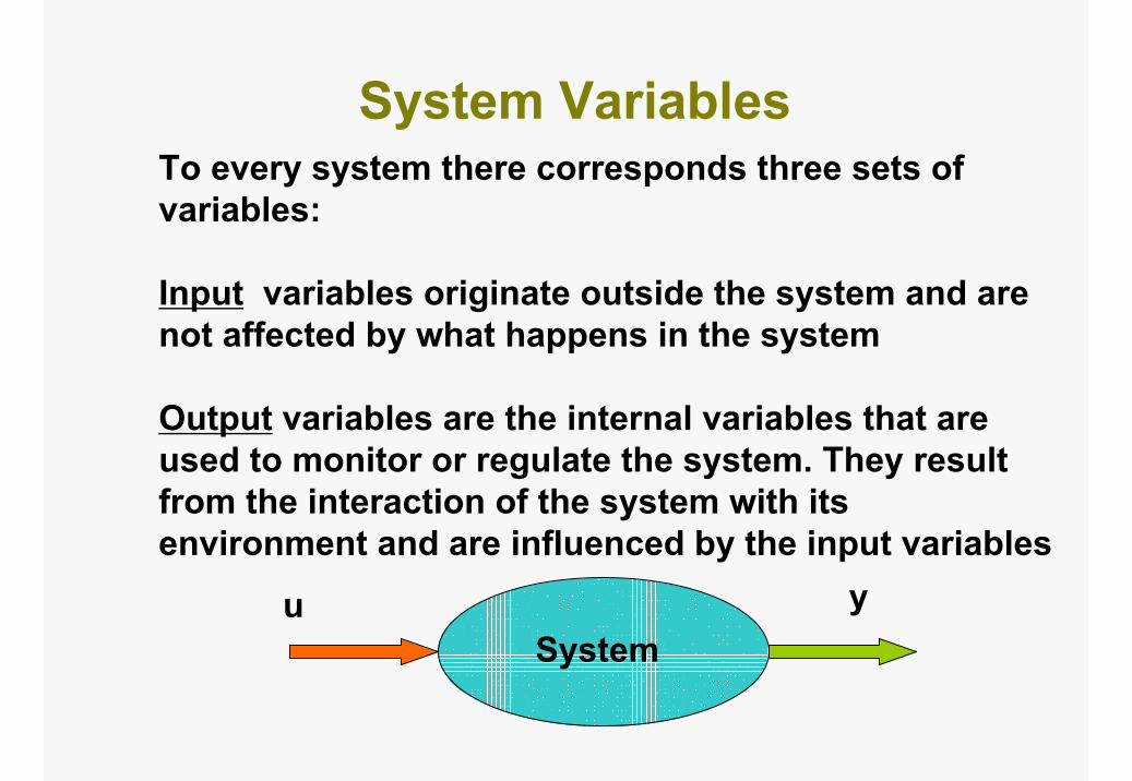
System VariablesTo every system there corresponds three sets of variables:

Input variables originate outside the system and are not affected by what happens in the system

Output variables are the internal variables that are used to monitor or regulate the system. They result from the interaction of the system with its environment and are influenced by the input variables

Systemu y

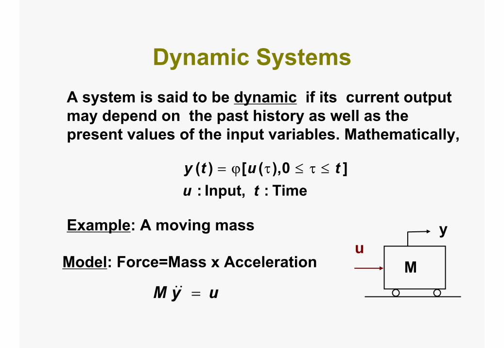
Dynamic SystemsA system is said to be dynamic if its current output may depend on the past history as well as the present values of the input variables. Mathematically,

Time : Input, :]0),([)(

tututy ≤τ≤τϕ=

Example: A moving mass

M

yu

Model: Force=Mass x Acceleration

uyM =

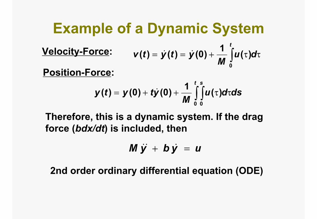
Example of a Dynamic SystemVelocity-Force: ∫ ττ+==

t

duM

ytytv0

)(1)0()()(

Therefore, this is a dynamic system. If the drag force (bdx/dt) is included, then

uybyM =+

2nd order ordinary differential equation (ODE)

Position-Force:

dsduM

ytytyt s

∫ ∫ ττ++=0 0

)(1)0()0()(

Mathematical Modeling BasicsMathematical model of a real world system is derived using analytical and experimental means

• Analytical model is derived based on governing physical laws for the system such as Newton's law, Ohms law, etc.

• It is often assembled into a single or system of differential (difference in the case of discrete-time systems) equations

• An analytical model maybe linear or nonlinear

Mathematical Modeling Basics

• A nonlinear model is often linearized about a certain operating point

• Model reduction (or approximation) may be needed to get a lumped-parameter (finite dimensional) model

• Numerical values of the model parameters are often approximated from experimental data by curve fitting.

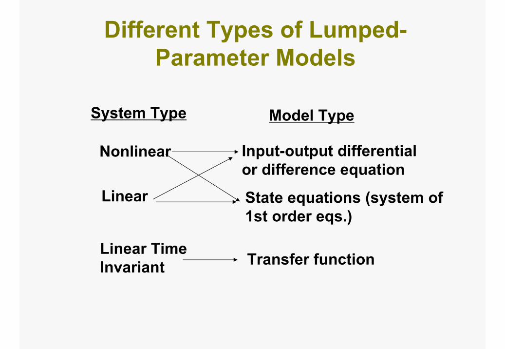
Different Types of Lumped-Parameter Models

Input-output differential or difference equation

State equations (system of 1st order eqs.)

Transfer function

Nonlinear

Linear

Linear Time Invariant

System Type Model Type

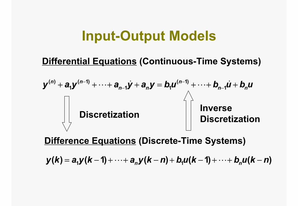
Input-Output Models Differential Equations (Continuous-Time Systems)

ubububyayayay nnn

nnnn +++=++++ −

−−

−1

)1(11

)1(1

)(

)()1()()1()( 11 nkubkubnkyakyaky nn −++−+−++−=

Difference Equations (Discrete-Time Systems)

DiscretizationInverse Discretization

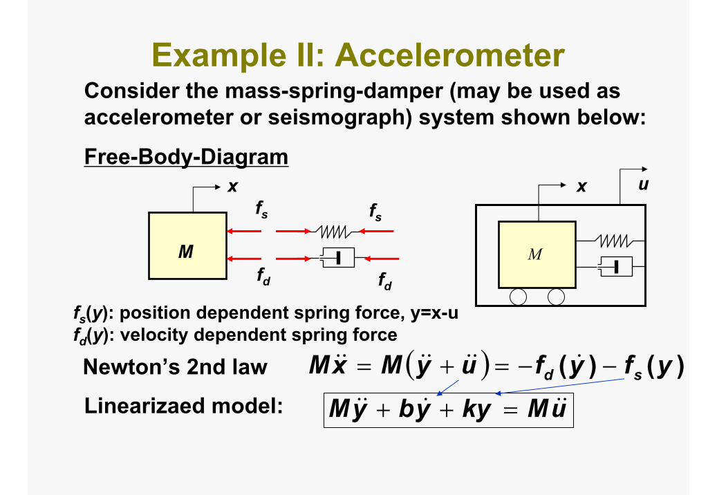
Example II: AccelerometerConsider the mass-spring-damper (may be used as accelerometer or seismograph) system shown below:

Free-Body-Diagram

M

fs

fd

fs

fd

x

fs(y): position dependent spring force, y=x-ufd(y): velocity dependent spring force

Newton’s 2nd law ( ) )()( yfyfuyMxM sd −−=+=

Linearizaed model: uMkyybyM =++

M

ux

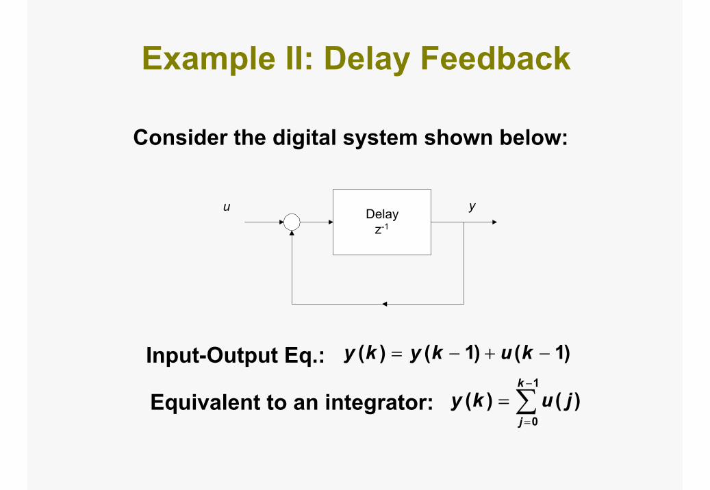
Example II: Delay Feedback

Delayz-1

u y

Consider the digital system shown below:

Input-Output Eq.: )1()1()( −+−= kukyky

Equivalent to an integrator: ∑−

=

=1

0)()(

k

jjuky

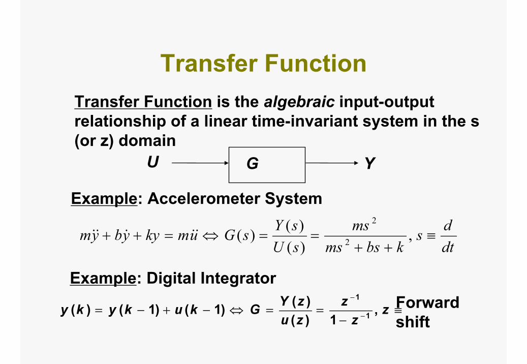
Transfer FunctionTransfer Function is the algebraic input-output relationship of a linear time-invariant system in the s (or z) domain

GU Y

dtds

kbsmsms

sUsYsGumkyybym ≡

++==⇔=++ ,

)()()( 2

2

Example: Accelerometer System

Example: Digital Integrator

≡−

==⇔−+−= −

−

zz

zzuzYGkukyky ,

1)()()1()1()( 1

1 Forward shift

Comments on TF

• Transfer function is a property of the system independent from input-output signal

• It is an algebraic representation of differential equations

• Systems from different disciplines (e.g., mechanical and electrical) may have the same transfer function

Mixed Systems

• Most systems in mechatronics are of the mixed type, e.g., electromechanical, hydromechanical, etc

• Each subsystem within a mixed system can be modeled as single discipline system first

• Power transformation among various subsystems are used to integrate them into the entire system

• Overall mathematical model may be assembled into a system of equations, or a transfer function

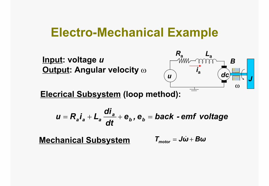
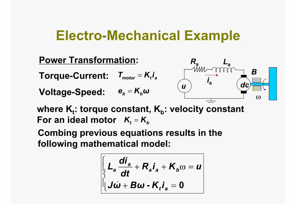
Electro-Mechanical Example

voltage emf-backe,edtdiLiRu bb

aaaa =++=

Mechanical Subsystem BωωJTmotor +=

uia dc

Ra La

Jω

BInput: voltage uOutput: Angular velocity ω

Elecrical Subsystem (loop method):

Electro-Mechanical Example

uia dc

Ra La

ω

Torque-Current:

Voltage-Speed:atmotor iKT =

Combing previous equations results in the following mathematical model:

BPower Transformation:

ωKe bb =

=+

=ω++

0at

baaa

a

iK-BωωJ

uKiRdtdiL

where Kt: torque constant, Kb: velocity constant For an ideal motor bt KK =

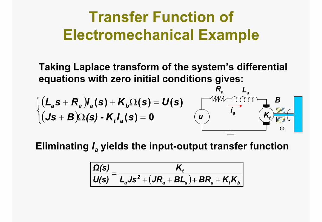
Transfer Function of Electromechanical Example

Taking Laplace transform of the system’s differential equations with zero initial conditions gives:

Eliminating Ia yields the input-output transfer function

( ) btaaa2

a

t

KKBRBLJRJsLK

U(s)Ω(s)

++++=

uia Kt

Ra La

ω

B( )( )

=Ω+=Ω++

0)()()()(

sIK-(s)BJssUsKsIRsL

at

baaa

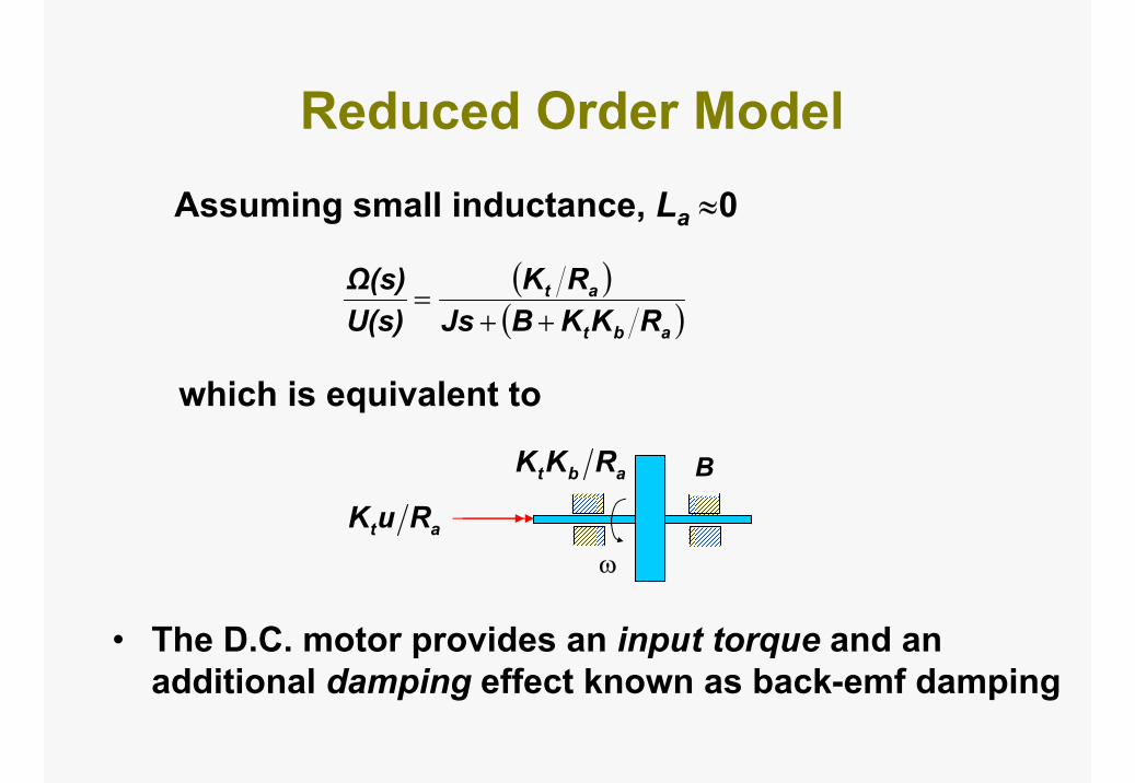
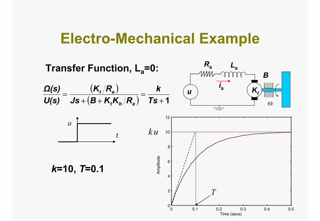
Reduced Order ModelAssuming small inductance, La ≈0

( )( )abt

at

RKKBJsRK

U(s)Ω(s)

++=

which is equivalent to

ωat RuK

Babt RKK

• The D.C. motor provides an input torque and an additional damping effect known as back-emf damping

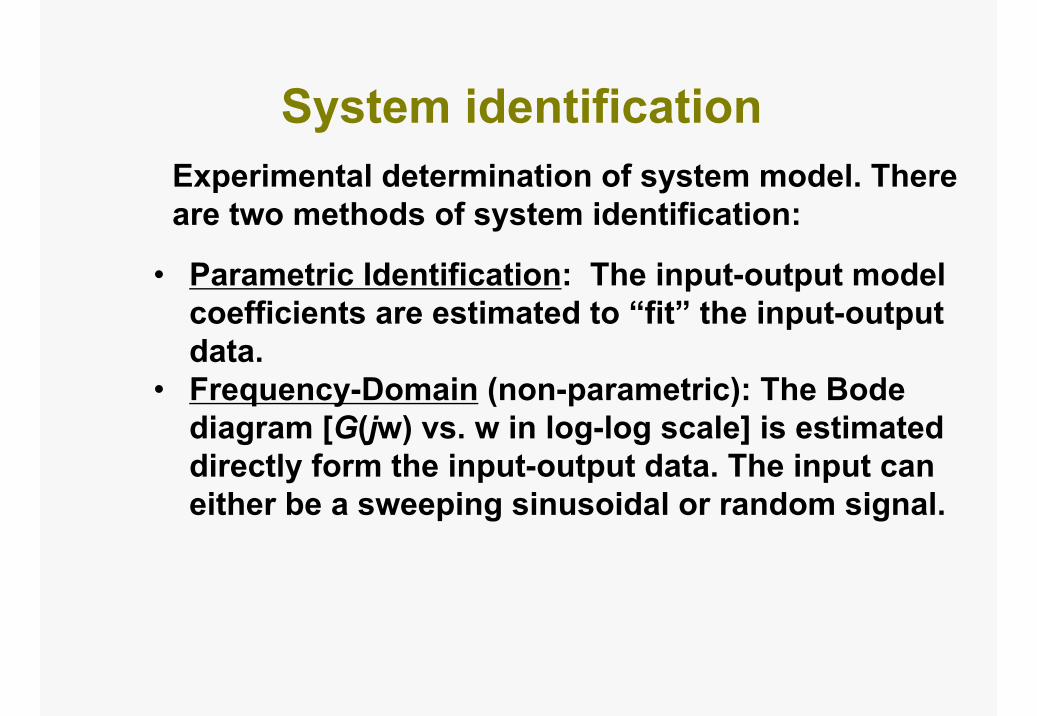
System identification

• Parametric Identification: The input-output model coefficients are estimated to “fit” the input-output data.

• Frequency-Domain (non-parametric): The Bode diagram [G(jw) vs. w in log-log scale] is estimated directly form the input-output data. The input can either be a sweeping sinusoidal or random signal.

Experimental determination of system model. There are two methods of system identification:

Electro-Mechanical Example

uia Kt

Ra La

ω

B

( )( ) 1+

=++

=Ts

kRKKBJs

RKU(s)Ω(s)

abt

at

Transfer Function, La=0:

0 0.1 0.2 0.3 0.4 0.50

2

4

6

8

10

12

Time (secs)

Ampl

itude

ku

T

u

t

k=10, T=0.1

Comments on First Order Identification

Graphical method is

• difficult to optimize with noisy data and multiple data sets

• only applicable to low order systems

• difficult to automate

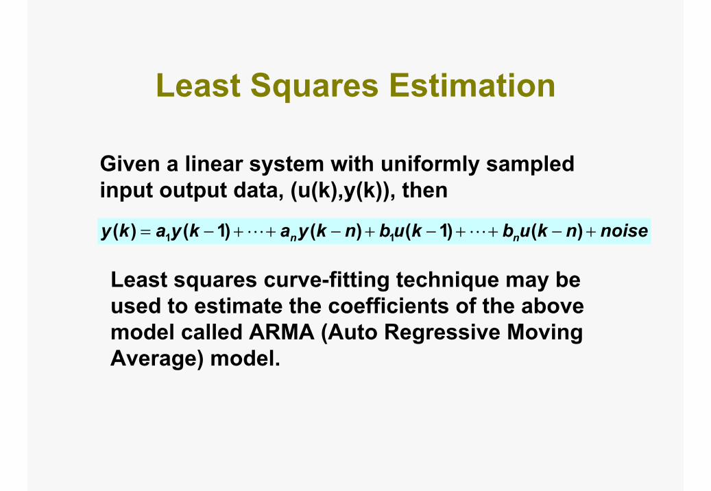
Least Squares Estimation

Given a linear system with uniformly sampled input output data, (u(k),y(k)), then

noisenkubkubnkyakyaky nn +−++−+−++−= )()1()()1()( 11

Least squares curve-fitting technique may be used to estimate the coefficients of the above model called ARMA (Auto Regressive Moving Average) model.

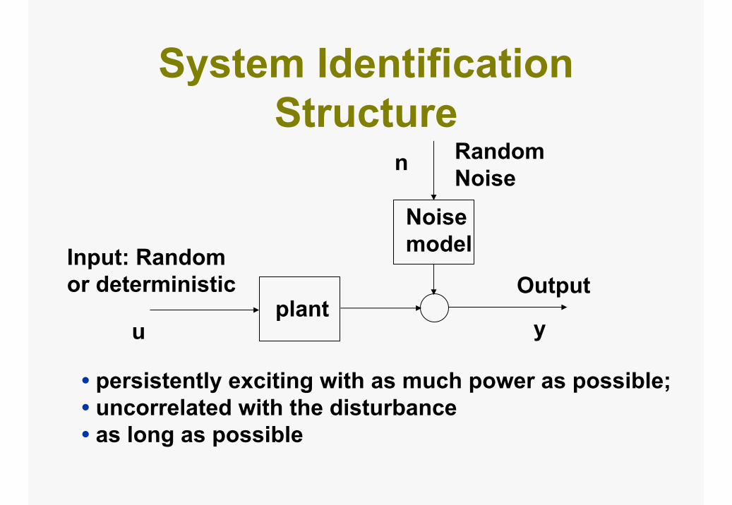
System Identification Structure

Input: Random or deterministic

Random Noise

u

Output

n

plant

Noise model

• persistently exciting with as much power as possible;• uncorrelated with the disturbance • as long as possible

y

Basic Modeling Approaches• Analytical

• Experimental

– Time response analysis (e.g., step, impulse)– Parametric

* ARX, ARMAX

* Box-Jenkins

* State-Space

– Nonparametric or Frequency based

* Spectral Analysis (SPA)

* Emperical Transfer Function Analysis (ETFE)

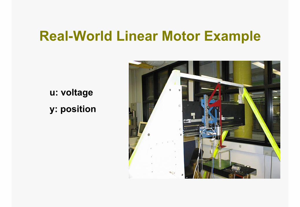
Real-World Linear Motor Example

u: voltage

y: position

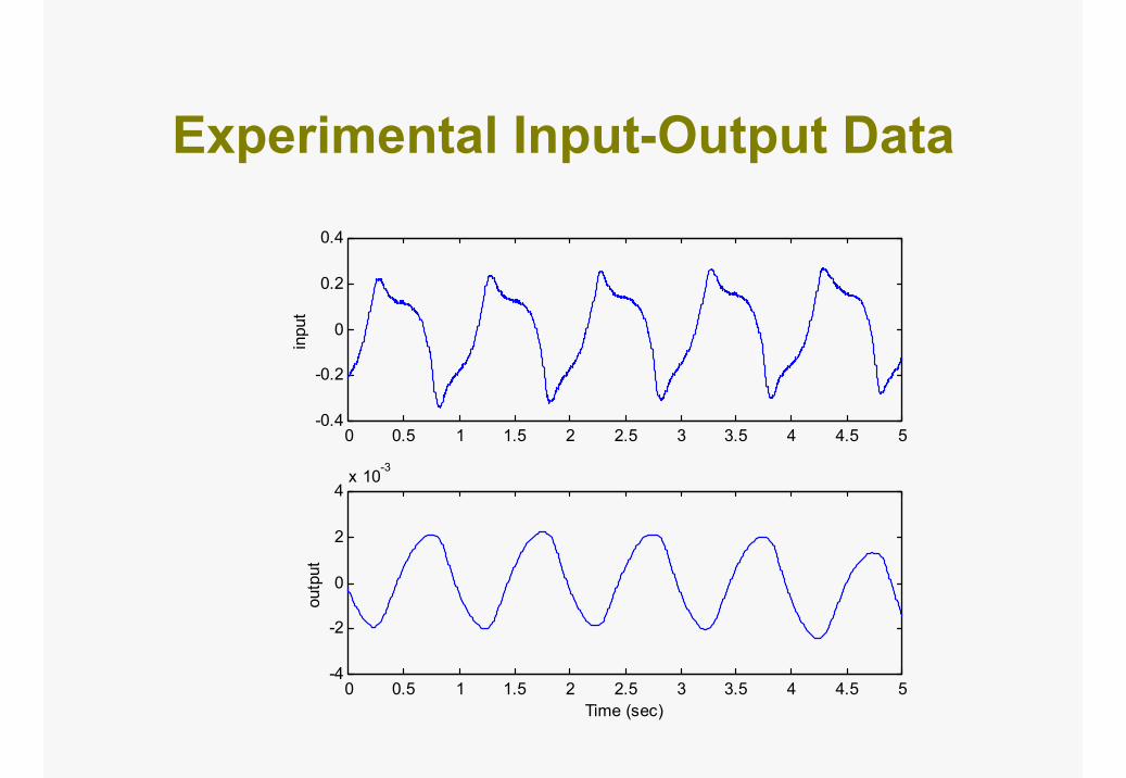
Experimental Input-Output Data

0 0.5 1 1.5 2 2.5 3 3.5 4 4.5 5-0.4

-0.2

0

0.2

0.4

inpu

t

0 0.5 1 1.5 2 2.5 3 3.5 4 4.5 5-4

-2

0

2

4x 10-3

Time (sec)

outp

ut

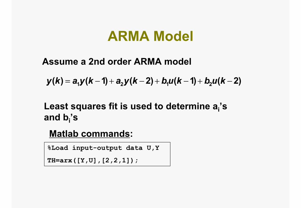
ARMA ModelAssume a 2nd order ARMA model

)2()1()2()1()( 2121 −+−+−+−= kubkubkyakyaky

Least squares fit is used to determine ai’sand bi’s

%Load input-output data U,Y

TH=arx([Y,U],[2,2,1]);

Matlab commands:

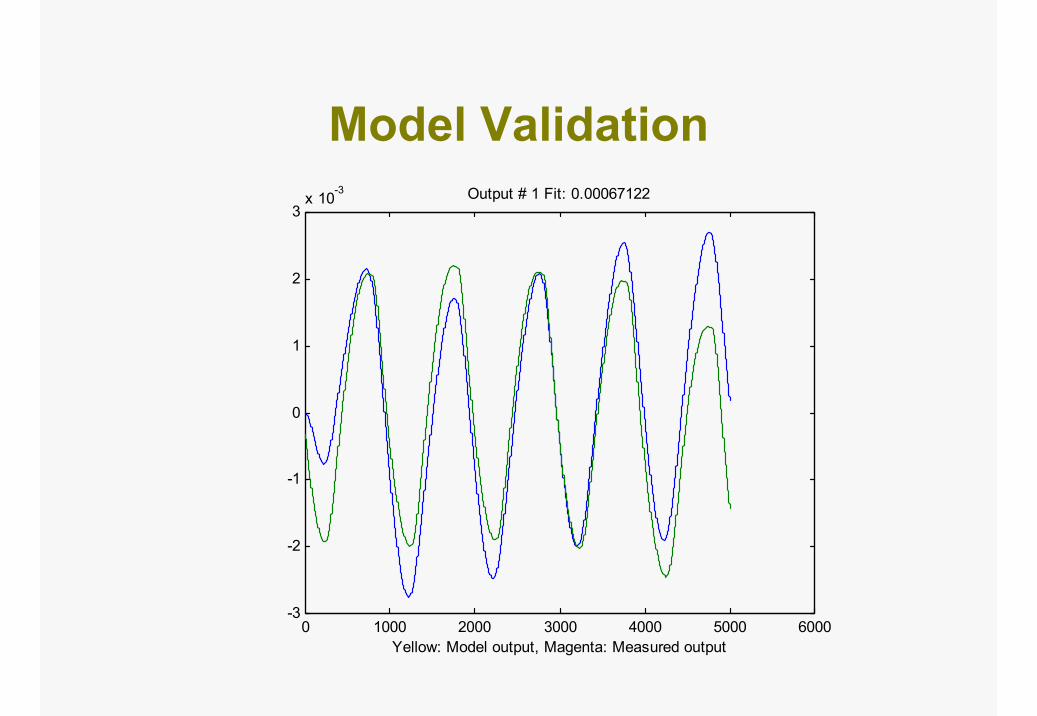
Model Validation

0 1000 2000 3000 4000 5000 6000-3

-2

-1

0

1

2

3x 10-3

Yellow: Model output, Magenta: Measured output

Output # 1 Fit: 0.00067122

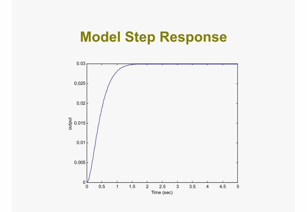
Model Step Response

0 0.5 1 1.5 2 2.5 3 3.5 4 4.5 50

0.005

0.01

0.015

0.02

0.025

0.03ou

tput

Time (sec)

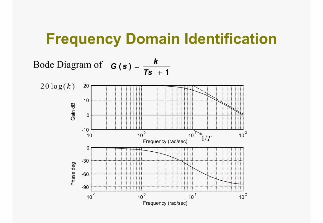
Frequency Domain IdentificationBode Diagram of

10-1

100

101

102-10

0

10

20

Frequency (rad/sec)

Gai

n dB

10-1

100

101

102

-30

-60

-90

0

Frequency (rad/sec)

Phas

e de

g

1/T

20 log ( )k

1)(

+=

TsksG

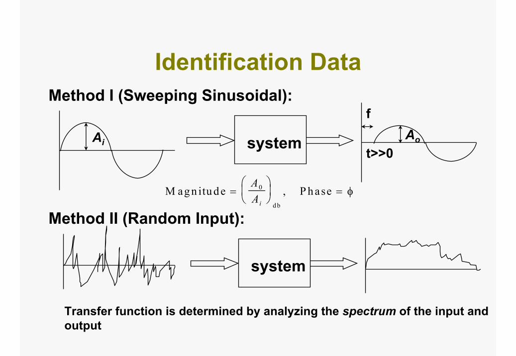
Identification DataMethod I (Sweeping Sinusoidal):

systemAi Ao

f

t>>0

M agn itu de P hased b

=

=

AAi

0 , φ

Method II (Random Input):

system

Transfer function is determined by analyzing the spectrum of the input and output

Random Input Method• Pointwise Estimation:

)()()(

ωω

=ωUYjG

This often results in a very nonsmooth frequency response because of data truncation and noise.

• Spectral estimation: uses “smoothed” sample estimators based on input-output covariance and crosscovariance.

The smoothing process reduces variability at the expense of adding bias to the estimate

)(ˆ)(ˆ

)(ˆωΦ

ωΦ=ω

u

yujeG

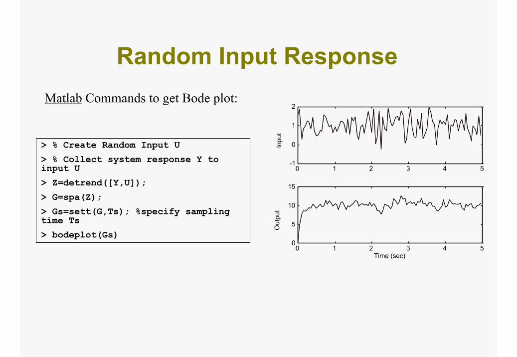
Matlab Commands to get Bode plot:

0 1 2 3 4 50

5

10

15

Time (sec)

Out

put

0 1 2 3 4 5-1

0

1

2

Inpu

t

> % Create Random Input U

> % Collect system response Y to input U

> Z=detrend([Y,U]);

> G=spa(Z);

> Gs=sett(G,Ts); %specify sampling time Ts

> bodeplot(Gs)

Random Input Response

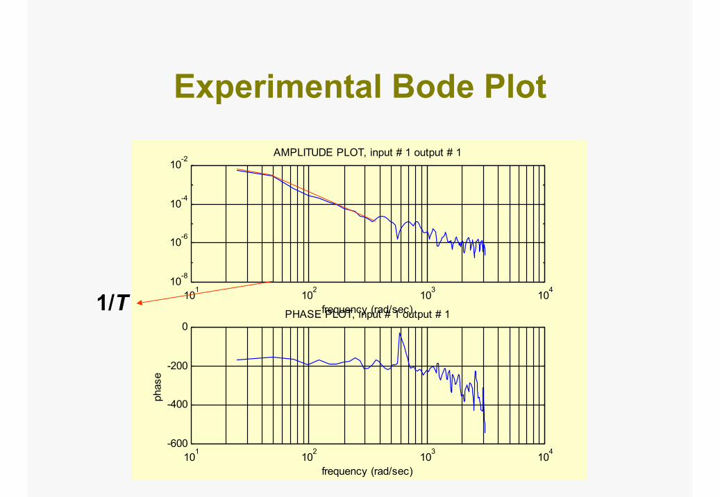
Experimental Bode Plot

101 102 103 10410-8

10-6

10-4

10-2

frequency (rad/sec)

AMPLITUDE PLOT, input # 1 output # 1

101 102 103 104-600

-400

-200

0PHASE PLOT, input # 1 output # 1

frequency (rad/sec)

phas

e

1/T

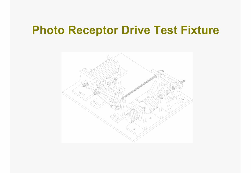
Photo Receptor Drive Test Fixture

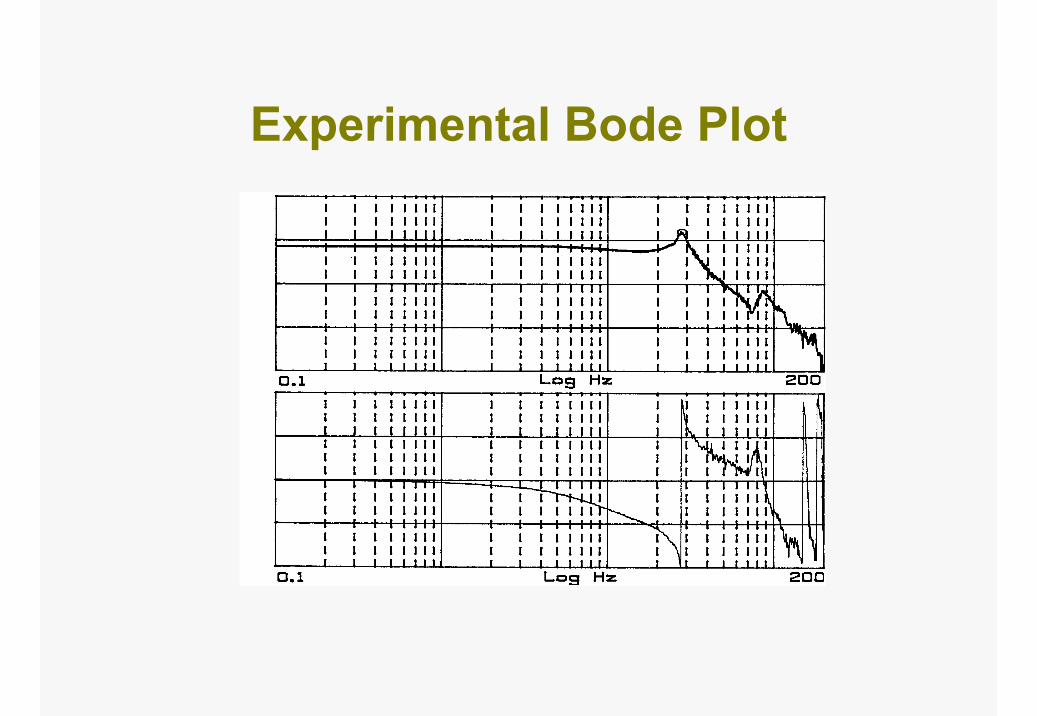
Experimental Bode Plot

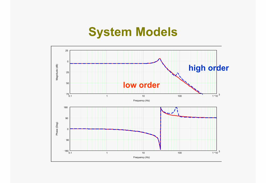
System Models

0.1 1 10 100 1 10 375

50

25

0

25

Frequency (Hz)

Mag

nitu

de (d

B)

0.1 1 10 100 1 10 3180

90

0

90

180

Frequency (Hz)

Phas

e (D

eg)

high order

low order