enabling technologies for sports (5xsf0) module...
TRANSCRIPT

1
1
Enabling Technologies for Sports /5XSF0 / Module 03 Freq. domain
PdW-SZ / 2017 Fac. EE SPS-VCA
Frequency domain processing
Sveta Zinger
Enabling Technologies for Sports (5XSF0)Module 3
2
Enabling Technologies for Sports /5XSF0 / Module 03 Freq. domain
PdW-SZ / 2017 Fac. EE SPS-VCA
Filtering in the frequency domain via the Fouriertransform– can be used for image enhancement, restoration,
compression
How to perform frequency domain processing inMatlab
What do we consider in frequency domain processing?
(The slides are based on “Digital Image Processing Using Matlab”, R. C. Gonzalez, R. E. Woods, S. L. Eddins)

2
3
Enabling Technologies for Sports /5XSF0 / Module 03 Freq. domain
PdW-SZ / 2017 Fac. EE SPS-VCA
2D Discrete Fourier Transform
For image f(x,y) (x=0,1,2,…,M-1 and
y=0,1,2,…,N-1), discrete Fourier transform (DFT) is
where u=0,1,2,…,M-1 and v=0,1,2,…,N-1
Frequency domain is the coordinate system spanned by F(u,v) with u and v as frequency variables
1
0
1
0
)//(2),(),(M
x
N
y
NvyMuxjeyxfvuF
4
Enabling Technologies for Sports /5XSF0 / Module 03 Freq. domain
PdW-SZ / 2017 Fac. EE SPS-VCA
Inverse Discrete Fourier Transform
Inverse DFT is given by
where x=0,1,2,…,M-1 and y=0,1,2,…,N-1,
the values F(u,v) are called Fourier coefficients
F(0,0) is the DC component (Direct current – from electrical engineering) of the Fourier transform
1
0
1
0
)//(2),(1
),(M
u
N
v
NvyMuxjevuFMN
yxf

3
5
Enabling Technologies for Sports /5XSF0 / Module 03 Freq. domain
PdW-SZ / 2017 Fac. EE SPS-VCA
Analyzing a transform – (1)
Even if f(x,y) is real, the transform in general is complex
Spectrum – the magnitude of F(u,v) – is the principal method of visually analyzing a transform
Fourier spectrum is defined as
where R(u,v) and I(u,v) represent the real and imaginary components of F(u,v)
2122 ),(),(),( vuIvuRvuF
6
Enabling Technologies for Sports /5XSF0 / Module 03 Freq. domain
PdW-SZ / 2017 Fac. EE SPS-VCA
Analyzing a transform – (2)
Fourier spectrum is symmetric about the origin
DFT is infinitely periodic in both u and v directions, the periodicity is determined by M and N
Image obtained by taking the inverse DFT is also infinitely periodic; DFT implementations compute only one period – M x N
),(),( vuFvuF

4
7
Enabling Technologies for Sports /5XSF0 / Module 03 Freq. domain
PdW-SZ / 2017 Fac. EE SPS-VCA
Analyzing a transform – (3)
Transform is centered on the origin
Move the origin of the transform to the point u=M/2
8
Enabling Technologies for Sports /5XSF0 / Module 03 Freq. domain
PdW-SZ / 2017 Fac. EE SPS-VCA
Analyzing a transform – (4)
In Matlab, data is rearranged after the transform using fftshift

5
9
Enabling Technologies for Sports /5XSF0 / Module 03 Freq. domain
PdW-SZ / 2017 Fac. EE SPS-VCA
Computing and visualizing 2D DFT in Matlab
DFT and its inverse are obtained in practice using aFast Fourier Transform (FFT): F=fft2(f)– it is necessary to pad the input image with zeros: F=fft2(f,P,Q) – pads the input so that the resulting function is of size P x Q
– Fourier spectrum: S=abs(F)
– Inverse Fourier transform: f=ifft2(F);
– obtain an image containing only real values: f=real(ifft2(F))
10
Enabling Technologies for Sports /5XSF0 / Module 03 Freq. domain
PdW-SZ / 2017 Fac. EE SPS-VCA
Computing and visualizing 2D DFT in Matlab: example
F=fft2(f);S=abs(F);figure; imshow(S,[])
Fc=fftshift(F);figure; imshow(abs(Fc),[])
S2=log(1++abs(Fc));figure; imshow(S2,[])

6
11
Enabling Technologies for Sports /5XSF0 / Module 03 Freq. domain
PdW-SZ / 2017 Fac. EE SPS-VCA
Filtering in the frequency domain
and
Convolution theorem
symbol indicates convolutionH(u,v) – filter transfer function
vuFvuHyhhyxf ,,,,
vuFvuHyhhyxf ,,,, ""
Frequency domain filtering: select a filter transferfunction that modifies F(u,v) in a specifiedmanner
12
Enabling Technologies for Sports /5XSF0 / Module 03 Freq. domain
PdW-SZ / 2017 Fac. EE SPS-VCA
Transfer function for lowpass filter: example
after fftshift
Lowpass filter attenuates the high-frequency components of F(u,v), while leaving the low frequencies relatively unchanged.
Result of lowpass filtering is image blurring (smoothing).

7
13
Enabling Technologies for Sports /5XSF0 / Module 03 Freq. domain
PdW-SZ / 2017 Fac. EE SPS-VCA
Padding functions with zeros
For functions f(x,y) and h(x,y) of size A x B and C x D respectively,
form two extended (padded) functions, both of size P x Q, by
appending zeros to f and g.
Wraparound error is avoided by choosing and
If the functions are of the same size, M x N, then the padding values
are and
1 CAP
1 DBQ
12 MP 12 NQ
14
Enabling Technologies for Sports /5XSF0 / Module 03 Freq. domain
PdW-SZ / 2017 Fac. EE SPS-VCA
Basic steps (1-2) in DFT filtering
Step-by-step procedure involving Matlab functions, where f – image to be filtered, g – result, H(u,v) – filter function of the same size as the padded image.
1. Obtain the padding parameters: PQ=2*size(f).
2. Obtain the Fourier transform with padding: F=fft2(f,PQ(1),PQ(2)).

8
15
Enabling Technologies for Sports /5XSF0 / Module 03 Freq. domain
PdW-SZ / 2017 Fac. EE SPS-VCA
Basic steps (3-6) in DFT filtering
3. Generate a filter function H of size PQ1 x PQ2. If the filter function is centered, let H=fftshift(H)before using the filter.
4. Multiply the transform by the filter: G=H.*F;
5. Obtain the real part of the inverse FFT of G: g=real(ifft2(G));
6. Crop the top left rectangle of the original size: g=g(1:size(f,1),1:size(f,2));
16
Enabling Technologies for Sports /5XSF0 / Module 03 Freq. domain
PdW-SZ / 2017 Fac. EE SPS-VCA
Filtering procedure summarized

9
17
Enabling Technologies for Sports /5XSF0 / Module 03 Freq. domain
PdW-SZ / 2017 Fac. EE SPS-VCA
Converting spatial filters into equivalent frequency domain filters
Choice between filtering in spatial or frequencydomain may depend on the computational efficency
Filter in the frequency domain:H=freqz2(h,R,C),where h is a 2D spatial filter,
R is the number of rows and
C is the number of columns that we wish filter H to have
18
Enabling Technologies for Sports /5XSF0 / Module 03 Freq. domain
PdW-SZ / 2017 Fac. EE SPS-VCA
Spatial filtering (Sobel) versus equivalent frequency domain filtering:
identical results
initial image spatial filtering frequency domain filtering
(thresholded results)

10
19
Enabling Technologies for Sports /5XSF0 / Module 03 Freq. domain
PdW-SZ / 2017 Fac. EE SPS-VCA
Creating meshgrid arrays for filters in the frequency domain
function [U V]=dftuv(M,N)
% DFTUV Computes meshgrid frequency matrices. U and V are both M-by-N
% Set up range of variables
u=0:(M-1); v=0:(N-1);
% Compute the indices for use in meshgrid
idx=find(u>M/2); u(idx)=u(idx)-M;
idy=find(v>N/2); v(idy)=v(idy)-N;
% Compute the meshgrid arrays
[U V]=meshgrid(v,u);
20
Enabling Technologies for Sports /5XSF0 / Module 03 Freq. domain
PdW-SZ / 2017 Fac. EE SPS-VCA
Lowpass frequency domain filters – (1)
Ideal lowpass filter (ILPF) has the transfer function
where D0 – specified nonnegative number,
D(u,v) – distance from point (u,v) to the center of the filter
– Ideal filter “cuts off” (multiplies by 0) all components of Foutside the circle and leaves unchanged (multiplies by 1) all components on, or inside, the circle
0
0
,if0
,if1,
DvuD
DvuDvuH

11
21
Enabling Technologies for Sports /5XSF0 / Module 03 Freq. domain
PdW-SZ / 2017 Fac. EE SPS-VCA
Lowpass frequency domain filters – (2)
Butterworth lowpass filter (BLPF) of order n, with acutoff frequency at a distance D0 from the origin,has the transfer function
– BLPF transfer function does not have a sharp discontinuity at D0
nDvuD
vuH 20,1
1,
22
Enabling Technologies for Sports /5XSF0 / Module 03 Freq. domain
PdW-SZ / 2017 Fac. EE SPS-VCA
Lowpass frequency domain filters – (3)
Transfer function of a Gaussian lowpass filter(GLPF)
where – standard deviation
– By letting , we obtain the expression for GLPF in terms of the cutoff parameter:
22 2,, vuDevuH
0D
20
2 2,, DvuDevuH

12
23
Enabling Technologies for Sports /5XSF0 / Module 03 Freq. domain
PdW-SZ / 2017 Fac. EE SPS-VCA
Gaussian lowpass filter: example – (1)PQ=2*size(f);
% Create meshgrid for the transfer function – you need dftuv.m
[U V]=dftuv(PQ(1),PQ(2));
D=sqrt(U.^2+V.^2);
% define the parameter for cut-off frequency D0
D0=0.05*PQ(2); % 5% of the padded image width
% Perform FFT of the original image and obtain the filter transfer function
F=fft2(f,PQ(1),PQ(2));
H=exp(-(D.^2)/(2*(D0^2)));
% Obtain and crop the resulting image
g=real(ifft2(H.*F));
g=g(1:size(f,1),1:size(f,2));
24
Enabling Technologies for Sports /5XSF0 / Module 03 Freq. domain
PdW-SZ / 2017 Fac. EE SPS-VCA
Gaussian lowpass filter: example – (2)
Blurred version of the original
figure; imshow(fftshift(H),[])
figure; imshow(log(1++abs(fftshift(F))),[])
figure; imshow(g,[])

13
25
Enabling Technologies for Sports /5XSF0 / Module 03 Freq. domain
PdW-SZ / 2017 Fac. EE SPS-VCA
3D plots – (1)
Draw a plot: mesh, surf Set or switch off axis: axis Switch on or off the grid: grid Change the viewing point:
– view
– Click on the “Rotate 3D” button in the figure window’s toolbar
26
Enabling Technologies for Sports /5XSF0 / Module 03 Freq. domain
PdW-SZ / 2017 Fac. EE SPS-VCA
3D plots – (2)
14
27
Enabling Technologies for Sports /5XSF0 / Module 03 Freq. domain
PdW-SZ / 2017 Fac. EE SPS-VCA
Sharpening frequency domain filters: highpass filtering
Highpass filtering sharpens the image byattenuating the low frequencies and leaving thehigh frequencies of the Fourier transformrelatively unchanged
Transfer function of a highpass filter:
vuHvuH lphp ,1,
where Hlp(u,v) – transfer function of the corresponding lowpass filter
28
Enabling Technologies for Sports /5XSF0 / Module 03 Freq. domain
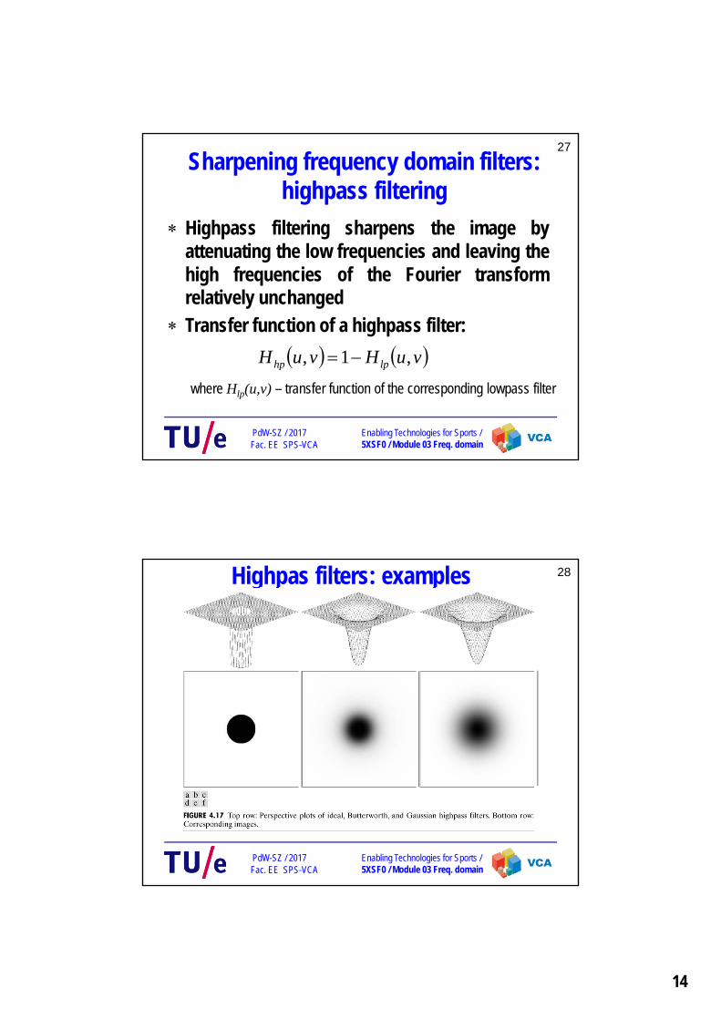
PdW-SZ / 2017 Fac. EE SPS-VCA
Highpas filters: examples

15
29
Enabling Technologies for Sports /5XSF0 / Module 03 Freq. domain
PdW-SZ / 2017 Fac. EE SPS-VCA
Reference
– Rafael C. Gonzalez, Richard E. Woods, Steven L. Eddins, “Digital Image Processing Using Matlab”, Pearson Education, 2004
– Chapter 4