EnergyPLAN

Advanced Energy Systems Analysis Computer Model

February 2010

Documentation Version 8.0 Henrik Lund Aalborg University Denmark

Energy PLAN Advanced Energy System Analysis Computer Model

2

3

Preface The EnergyPLAN model has been developed and expanded into the version 7.0 in the period since year 1999. Initially, the model was developed by Henrik Lund and implemented in an EXCEL spreadsheet. Very soon, the model grew huge, and consequently, in 2001, the primary programming of the model was transformed into visual basic (from version 3.0 to 4.4). At the same time, all the hour by hour distribution data were transformed into external text files. Altogether, this reduced the size of the model by a factor 30. This transformation was done in collaboration with Leif Tambjerg and Ebbe Münster (PlanEnergi consultants). During 2002, the model was re-programmed in Delphi Pascal into version 5.0. And during 2003, the model has been expanded into version 6.0. This transformation was implemented by Henrik Lund with the help and assistance of Anders N. Andersen and Henning Mæng (Energy and Environmental Data). In version 6.0, the model was expanded with a possibility of calculating the influence of CO2 emissions and the share of RES when the electricity supply is seen as a part of the total energy system of a region. Further possibilities of analysing different trade options on the external electricity market were added. During the spring of 2005, the model was expanded into version 6.2 in a comparative study with the H2RES model with a focus on energy system analysis of renewable islands. The comparative study was done together with Neven Duic and Goran Krajacić from University of Zagreb. As part of the work, two new possibilities of storing/converting electricity storage facilities were added to the EnergyPLAN model. The one is an electricity storage unit, which can be used for modelling e.g. hydro storage or battery storage. The other is electrolysers which are able to produce fuel (e.g. hydrogen) and heat for district heating. Moreover, the facility of modelling V2Gs (Vehicle to grid) was implemented in corporation with Willet Kempton from University of Delaware. During the autumn of 2005 and the spring of 2006, the model was expanded further into version 6.6. The main focus was to be able to do modelling of the energy systems of six European countries as part of the EU project DESIRE. Consequently, the possibility of selecting more renewable units, nuclear power and hydro power with water storage and reversible pump facilities was added to the system. During the summer and autumn of 2006, the model has been expanded further into the present version 7.0. New components such as different transportation options and different individual heating options have been added. A detailed model of Compressed Air Energy Systems (CAES) has been implemented by the help of PhD student Georges Salgi. Different options of waste utilisation have been added and tested by the help of PhD student Marie Münster. However, the primary achievement has been to implement a new economic regulation of the total energy system on the basis of the optimisation of the business-economic marginal production costs of each component in the system. An option to calculate total annual socio-economic costs has also been added. The new options have been tested and applied to an Energy Plan 2030 for Denmark by the help of PhD student Brian Vad Mathiesen.Diagrams of the expanded energy model have been made and implemented into the user interface with the assistance of Mette Reiche Sørensen, Aalborg University, who has also assisted in the writing of this documentation. Version 8 include new facilities of waste-to-energy technologies in combination with geothermal and absorption heat pumps develop by the help of Poul Østergaard, new facilities of Pump-Hydro-Energy-Storage helped by David Connolly together with a number of small improvements initiated by Poul Østergaard and Brian Vad Mathiesen. Among others it has become an option to store COST data alone. Henrik Lund, Aalborg University, February 2010

4

Content 1. Nomenclature 2. Introduction 2.1 Purpose and application 2.2 Energy Systems Analysis in the EnergyPLAN model 2.3 Energy Demands 2.4 Overview: Components and regulation 3. Libraries and settings

3.1 Input data set 3.2 Distribution 3.3 Cost database 3.4 Settings

4. Energy System Definition (Inputs)

4.1 Electricity Demand 4.2 District Heating 4.3 Renewable Energy Sources 4.4 ElecStorage 4.5 Cooling 4.6 Individual 4.7 Industry 4.8 Transport 4.9 Waste 4.10 Biomass 4.11 Fuel Cost 4.12 Operation Cost 4.13 Investment Cost 4.14 Additional Investments 4.15 Regulation

5. Initial analyses not involving electricity balancing

5.1 Fixed import/export of electricity 5.2 District heating demands incl. heat demands from absorption cooling 5.3 District heating and electricity productions from Industry and Waste 5.4 Fixed Boiler production subtracted from the district heating demand 5.5 Boiler production in district heating group 1

6. Technical Energy System Analysis 6.1 Condensing power and import/export including CEEP and EEEP 6.2 CHP, Heat Pumps and boilers in groups 2 and 3 (regulation 1 or 4) 6.3 Flexible electricity demand (including dump charge of BEV) 6.4 CHP, Heat Pumps and boilers in groups 2 and 3 (regulation 2 or 3) 6.5 Hydro power 6.6 Individual CHP and Heat Pump systems 6.7 Electrolyser for micro CHP, Transportation, DH groups 2 and 3 6.8 Heat storage in groups 2 and 3 6.9 Transportation (smart charge and V2G) 6.10 Electricity storage

5

7. Market-Economic Optimisation 7.1 Net import and resulting external market price 7.2 The overall procedure 7.3 CHP3 minimum production 7.4 District heating supplied by solar thermal and boilers 7.5 Hydrogen and electricity demands for transportation and micro CHP 7.6 Electricity Consumption from Heat Pumps and DH electrolysers 7.7 Hydro Power 7.8 Electricity Consumption from Heat Pumps and DH electrolysers 7.9 Electricity storage (Hydro or battery or CAES storage) 7.10 Resulting electricity market prices (External, Domestic and bottlenecks) 7.11. Grid stability

8. Fuel, CO2 emission and Feasibility Study (calculations) 8.1 Fixed boiler production is added to the boilers in groups 2 and 3 8.2 Reducing Critical Excess Electricity Production 8.3 Grid stabilisation 8.4 Heat balances in district heating systems 8.5 Fuel consumptions 8.6 CO2 emissions 8.7 Share of Renewable Energy

8.8 Cost 9. Output

9.1 The screen function 9.2 The print 9.3 Graphics 9.4 Run serial calculations function 9.5 Export Screen Data to Clipboard and e.g. EXCEL

10. Business optimisation of CAES plants

10.1 Theoretically optimal strategy 10.2 Practical operation strategies

6

Nomenclature Variables are used for demands, productions, efficiencies and similarly for various components such as electricity demands, boiler productions, etc. The demand and production unit specifications are given as indexes to the demands and productions. Annual demands and productions are written in capital letters such as Q and E. The hourly value is written in small letters such as q and e using the same alphabetic letters for the same demands. E.g. the capital letter D is used for annual electricity demands and the small letter d is used for hourly values of electricity demands. Such notation is short for the relation that the sum of 8784 hours of d’s during a year adds up to the value of capital D:

x=1

DE = Σ dE (x) 8784

Examples: DE, dFXDAY, hDH2, Annual Demands Hour demands D H F

Annual electricity Demand Annual Heat demand Annual Fuel demand/consumption

d h f

hour electricity demand hour heat demand hour fuel demand

Index E EH EC EX FXDay FXWeek FX4Week DH1 DH2 DH3 Cool Cool1 Cool2 Cool3 I V CSHP

Electricity demand Electricity heating demand Electricity cooling demand Fixed Exchange electricity demand Flexible demand (1 day) Flexible demand (1 week) Flexible demand (4 weeks) District Heating group 1 District Heating group 2 District Heating group 3 Cooling (electric grid) Cooling in DH1 Cooling in DH2 Cooling in DH3 Industry Various Industrial Combined Heat and Power

M-Coal M-Oil M-Ngas M-Bio M-H2CHP M-NgasCHP M-BioCHP M-HP M-EH T BEV V2G W1 W2 W3

Individual Coal boilers Individual Oil boilers Individual Natural gas boilers Individual Biomass boilers Micro Hydrogen CHP Micro Natural gas CHP Micro Biomass CHP Individual Heat Pump Individual Electric heating Transport Battery Electric Vehicle Vehicle to Grid Waste in DH1 Waste in DH2 Waste in DH3

7

Examples: CCHP2, eHP2, QB2, μCHP2, αELC2, Annual Productions

Hour productions

E Q F W

Annual electricity production Annual Heat production Annual Fuel demand/consumption Annual Water supply to Hydro

e q f w s

hour electricity production hour heat production hour fuel demand or production hour water supply hour energy content in storage

Capacities

Efficiencies

C T S LOSS SHARE FAC LIMIT Stab

Capacity (Electric) Capacity (Thermal) Capacity storage (Energy) Loss from storage Share of e.g. DH with Solar Correction Factor (e.g. RES prod.) Capacity limit of micro CHP etc. Grid stabilisation share

μ ρ φ α ψ η τ

electric (=electric/fuel) thermal (=heat/fuel) COP (=heat/elec) for HPs fuel (=fuel/elec) for electrolysers waste to fluid biofuels waste to solid biofuels waste to various (non energy) products

Index

Various factors

B1 B2 B3 CHP2 CHP3 HP2 HP3 PP Solar1 Solar2 Solar3 Res1 Res2

Boiler in DH group 1 Boiler in DH group 2 Boiler in DH group 3 Combined Heat Power in DH gr. 2 Combined Heat Power in DH gr. 3 Heat Pump in DH group 1 Heat Pump in DH group 2 Power plant (Condensing) Solar thermal in DH group 1 Solar thermal in DH group 2 Solar thermal in DH group 3 Renewable Energy Source 1 Renewable Energy Source 2

Res3 Res4 Hydro HydroPumpNuclear Geo Elc2 Elc3 ElcT ElcM Pump Turbine CAES

Renewable Energy Source 3 Renewable Energy Source 4Hydro power Reversible Hydro power Nuclear Geothermal Electrolyser in DH group 2 Electrolyser in DH group 3 Electrolyser for transportation Electrolyser for micro CHP Electricity storage charging unit Electricity storage discharge unit Compressed Air Energy Storage

Examples: PCoal-WM, PCoal-TaxI, CO2Coal, Annual Demands and prices Hour demands P A CO2

Average Annual price Annual Cost CO2 emissions

p n i

hour prices lifetime interest rate

Index WM HCen HDec HIndv HRoad HAir Unit

World Market Handling Costs to central level Handling Costs to decentralised Handling Costs to individual Handling Costs to road transport Handling Costs to Air transport Per unit prices

TaxIndv TaxI TaxB TaxCHP TaxCAES VOC FOC

Fuel Taxes for individuals Fuel Taxes for industry Fuel Taxes for Boilers Fuel Taxes for CHP Fuel Taxes for CAES storage Variable Operation Costs Fixed Operation Cost

8

2. Introduction The EnergyPLAN model is a computer model for Energy Systems Analysis. The model has been developed and expanded on a continuous basis since 1999. The analysis is carried out in hour by hour steps for one year. And the consequences are analysed on the basis of different technical regulation strategies as well as market-economic optimisation strategies. 2.1 Purpose and application The main purpose of the model is to assist the design of national energy planning strategies on the basis of technical and economic analyses of the consequences of different national energy systems and investments. The model emphasises the analysis of different regulation strategies with a focus on the interaction between combined heat and power production (CHP) and fluctuating renewable energy sources. The model is an input/output model. General inputs are demands, renewable energy sources, energy plant capacities, costs and a number of optional different regulation strategies emphasising import/export and excess electricity production. Outputs are energy balances and resulting annual productions, fuel consumption, import/exports and total costs including income from the exchange of electricity. The model can be used for different kinds of energy system analyses: Technical analysis Design and analysis of large and complex energy systems at the national level and under different technical regulation strategies. In this analysis, input is a description of energy demands, production capacities and efficiencies, and energy sources. Output consists of annual energy balances, fuel consumptions and CO2 emissions. Market exchange analysis Further analysis of trade and exchange on international electricity markets. In this case, the model needs further input in order to identify the prices on the market and to determine the response of the market prices to changes in import and export. Input is also needed in order to determine marginal production costs of the individual electricity production units. The modelling is based on the fundamental assumption that each plant optimises according to business-economic profits, including any taxes and CO2 emissions costs. Feasibility Studies Calculation of feasibility in terms of total annual costs of the system under different designs and regulation strategies. In such case, inputs such as investment costs and fixed operation and maintenance costs have to be added together with life time periods and an interest rate. The model determines the socio-economic consequences of the productions. The costs are divided into 1) fuel costs, 2) variable operation costs, 3) investment costs, 4) fixed operation costs, 5) electricity exchange costs and benefits, and 5) possible CO2 payments. The principle of the energy system of the EnergyPLAN model is shown in the diagram on the front page. Basically, the input of the energy system consists of the following:

- Energy demands (heat, electricity, transportation etc.) - Energy production units and resources (wind turbines, power plants, oil boilers, storage etc.) - Regulation (defining the regulation and operation of each plant and the system including

technical limitations such as transmission capacity etc.)

9

- Costs (Fuel costs, taxes, variable and fixed operation costs and investment costs) Basically, the model distinguishes between technical regulation and market-economic regulation. In the following, a list of energy demands is presented as well as an overview of all components in the model together with a short description on how they are operated in the two different regulation strategies. Also the main inputs for each component are listed. 2.2 Energy Systems Analysis in the EnergyPLAN model The procedure of the energy system analysis is shown in the diagram. The calculations are based on the small calculation described in the previous section, which is made simultaneously with the typing of input data in the input and cost windows. Next step consists of some initial calculations, which do not involve electricity balancing. Then the procedure is divided into EITHER a technical OR a market -economic optimisation. The technical optimisation minimises the import/export of electricity and seeks to identify the least fuel-consuming solution. On the other hand, the market-economic optimisation identifies the lowest cost solution on the basis of the business-economic costs of each production unit.

Step 1: Calculation from the input windows:

1. Electricity demand is calculated as in input window section 4.1.1 2. Solar thermal as in section 4.2.1 3. RES1, … RES4 as in section 4.3.1 4. Hydro Power input as in section 4.3.2 5. Nuclear Power or Geothermal as in section 4.3.3

Step 1 (Chapter 4): Calculation from the input windows

Step 2 (Chapter 5): Initial calculations not involving electricity

Step 4 (Chapter 8): CEEP regulation, Fuel, CO2 and Cost

EITHER Step 3A (Chapter 6):

Technical Energy System Optimisation

OR Step 3B (Chapter 7):

Market-Economic Energy System Optimisation

10

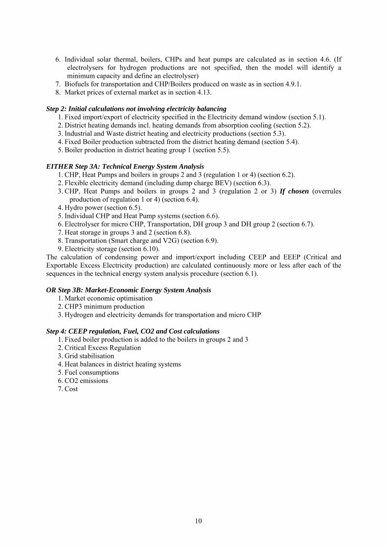
6. Individual solar thermal, boilers, CHPs and heat pumps are calculated as in section 4.6. (If electrolysers for hydrogen productions are not specified, then the model will identify a minimum capacity and define an electrolyser)

7. Biofuels for transportation and CHP/Boilers produced on waste as in section 4.9.1. 8. Market prices of external market as in section 4.13.

Step 2: Initial calculations not involving electricity balancing 1. Fixed import/export of electricity specified in the Electricity demand window (section 5.1). 2. District heating demands incl. heating demands from absorption cooling (section 5.2). 3. Industrial and Waste district heating and electricity productions (section 5.3). 4. Fixed Boiler production subtracted from the district heating demand (section 5.4). 5. Boiler production in district heating group 1 (section 5.5).

EITHER Step 3A: Technical Energy System Analysis

1. CHP, Heat Pumps and boilers in groups 2 and 3 (regulation 1 or 4) (section 6.2). 2. Flexible electricity demand (including dump charge BEV) (section 6.3). 3. CHP, Heat Pumps and boilers in groups 2 and 3 (regulation 2 or 3) If chosen (overrules

production of regulation 1 or 4) (section 6.4). 4. Hydro power (section 6.5). 5. Individual CHP and Heat Pump systems (section 6.6). 6. Electrolyser for micro CHP, Transportation, DH group 3 and DH group 2 (section 6.7). 7. Heat storage in groups 3 and 2 (section 6.8). 8. Transportation (Smart charge and V2G) (section 6.9). 9. Electricity storage (section 6.10).

The calculation of condensing power and import/export including CEEP and EEEP (Critical and Exportable Excess Electricity production) are calculated continuously more or less after each of the sequences in the technical energy system analysis procedure (section 6.1). OR Step 3B: Market-Economic Energy System Analysis

1. Market economic optimisation 2. CHP3 minimum production 3. Hydrogen and electricity demands for transportation and micro CHP

Step 4: CEEP regulation, Fuel, CO2 and Cost calculations

1. Fixed boiler production is added to the boilers in groups 2 and 3 2. Critical Excess Regulation 3. Grid stabilisation 4. Heat balances in district heating systems 5. Fuel consumptions 6. CO2 emissions 7. Cost

11

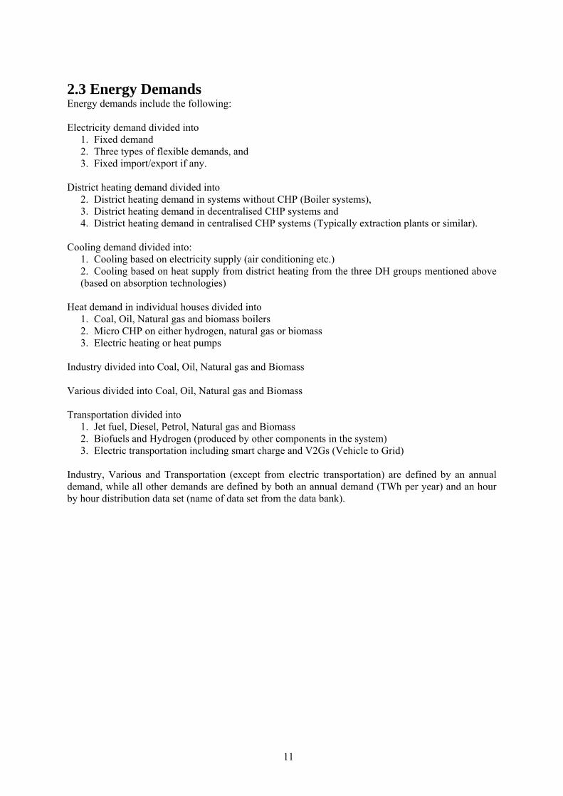
2.3 Energy Demands Energy demands include the following: Electricity demand divided into

1. Fixed demand 2. Three types of flexible demands, and 3. Fixed import/export if any.

District heating demand divided into

2. District heating demand in systems without CHP (Boiler systems), 3. District heating demand in decentralised CHP systems and 4. District heating demand in centralised CHP systems (Typically extraction plants or similar).

Cooling demand divided into:

1. Cooling based on electricity supply (air conditioning etc.) 2. Cooling based on heat supply from district heating from the three DH groups mentioned above (based on absorption technologies)

Heat demand in individual houses divided into

1. Coal, Oil, Natural gas and biomass boilers 2. Micro CHP on either hydrogen, natural gas or biomass 3. Electric heating or heat pumps

Industry divided into Coal, Oil, Natural gas and Biomass

Various divided into Coal, Oil, Natural gas and Biomass Transportation divided into

1. Jet fuel, Diesel, Petrol, Natural gas and Biomass 2. Biofuels and Hydrogen (produced by other components in the system) 3. Electric transportation including smart charge and V2Gs (Vehicle to Grid)

Industry, Various and Transportation (except from electric transportation) are defined by an annual demand, while all other demands are defined by both an annual demand (TWh per year) and an hour by hour distribution data set (name of data set from the data bank).

12

2.4 Overview: Components and Regulation Renewable Energy Sources Component Input Technical regulation Market-economic regulation Wind power Offshore wind Photovoltaic Wave power River Hydro

Electric capacity and Hourly distribution

Are given priority in the electricity production

Are given priority in the electricity production. Marginal production costs are defined as zero.

Hydro power Electric capacity Efficiency Storage capacity Annual Water supply Hourly distribution of water Variable operation costs

First, best possible utilisation of all water input given limitations in capacities is calculated and used as input. Afterwards Hydro power is relocated in the best possible way to avoid excess electricity production.

Identify highest possible production given water input and distribution, turbine capacity and water storage capacity. Sell such maximum production at the highest possible market prices to achieve the highest possible income.

Reversible Hydro Power

Same input as Hydro plus Pump Capacity Pump Efficiency Pump variable opr. Costs

Same as Hydropower plus In the end, the Pump is used in order to avoid excess electricity production and the Turbine to avoid production on condensing power plants.

Same as Hydro power plus The hydro power pump and turbine are used to optimise the profit of the plant based on marginal costs and losses in the energy conversion

Geothermal Power

Electric capacity Efficiency Hourly distribution Variable operation costs

Is given priority in the electricity production.

Produce whenever the electricity price is higher than the variable operation costs.

Solar thermal in district heating system

For each three DH groups: Annual production Hourly distribution Heat storage capacity Losses in heat storage

Is given priority in the district heating supply.

Is given priority in the heat production. Marginal production costs are defined as zero.

Solar thermal in individual houses

For each nine groups: Annual production Hourly distribution Heat storage capacity

Is given priority in the heat supply.

Is given priority in the heat production. Marginal production costs are defined as zero.

Waste utilisation and conversion and industrial electricity and heat production for district heating Component Input Technical regulation Market-economic regulation Industrial CHP Annual production and

Hourly distribution

Is given priority in the electricity production

Is given priority in the electricity production. Marginal production costs are defined as zero.

Industrial waste heat for district heating

For each three DH groups: Annual production and Hourly distribution

Is given priority in the district heating supply secondary to solar thermal.

Is given priority in the heat production secondary to solar thermal. Marginal production costs are defined as zero.

Waste incineration

For each three DH groups: Annual waste input and Hourly distribution Plant efficiency (thermal)

Is given priority in the district heating supply secondary to solar thermal.

Is given priority in the heat production secondary to solar thermal. Marginal production costs are defined as zero.

13

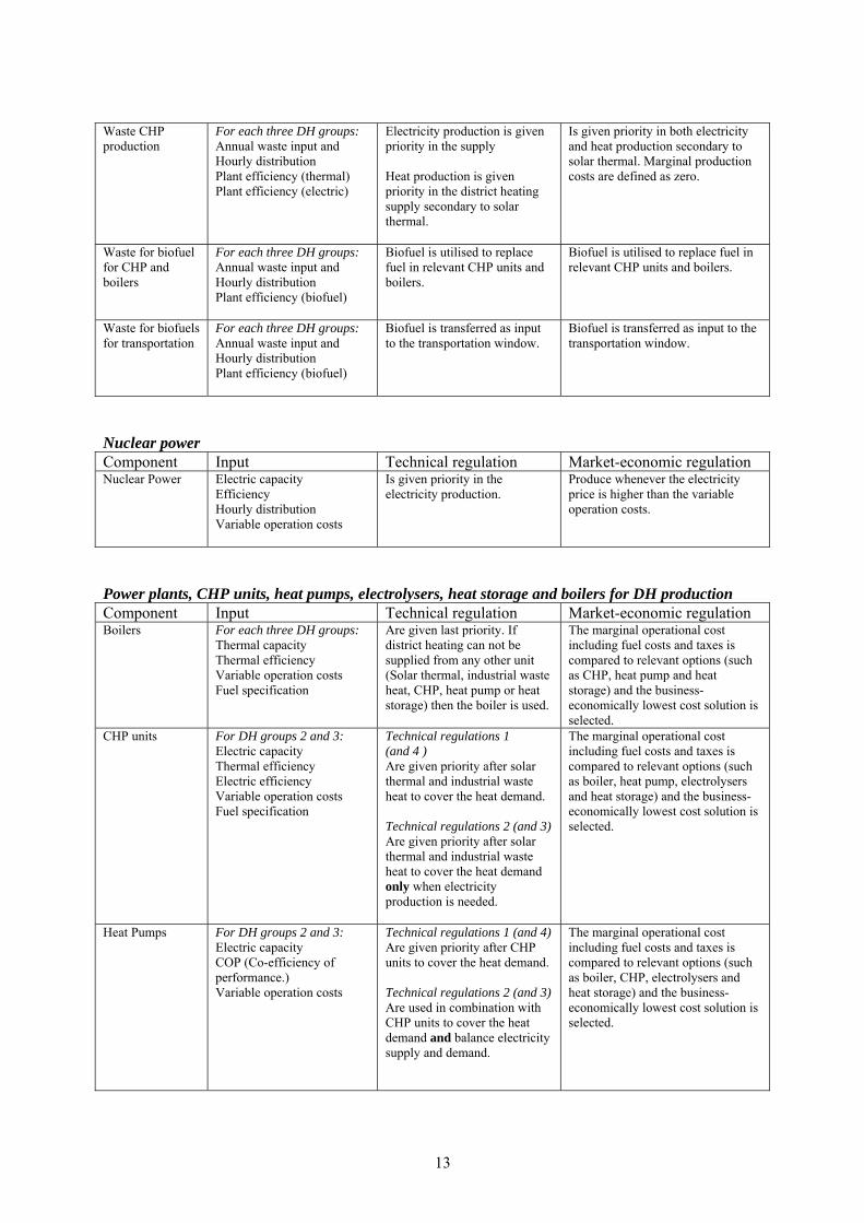
Waste CHP production

For each three DH groups: Annual waste input and Hourly distribution Plant efficiency (thermal) Plant efficiency (electric)

Electricity production is given priority in the supply Heat production is given priority in the district heating supply secondary to solar thermal.

Is given priority in both electricity and heat production secondary to solar thermal. Marginal production costs are defined as zero.

Waste for biofuel for CHP and boilers

For each three DH groups: Annual waste input and Hourly distribution Plant efficiency (biofuel)

Biofuel is utilised to replace fuel in relevant CHP units and boilers.

Biofuel is utilised to replace fuel in relevant CHP units and boilers.

Waste for biofuels for transportation

For each three DH groups: Annual waste input and Hourly distribution Plant efficiency (biofuel)

Biofuel is transferred as input to the transportation window.

Biofuel is transferred as input to the transportation window.

Nuclear power Component Input Technical regulation Market-economic regulation Nuclear Power Electric capacity

Efficiency Hourly distribution Variable operation costs

Is given priority in the electricity production.

Produce whenever the electricity price is higher than the variable operation costs.

Power plants, CHP units, heat pumps, electrolysers, heat storage and boilers for DH production Component Input Technical regulation Market-economic regulation Boilers For each three DH groups:

Thermal capacity Thermal efficiency Variable operation costs Fuel specification

Are given last priority. If district heating can not be supplied from any other unit (Solar thermal, industrial waste heat, CHP, heat pump or heat storage) then the boiler is used.

The marginal operational cost including fuel costs and taxes is compared to relevant options (such as CHP, heat pump and heat storage) and the business-economically lowest cost solution is selected.

CHP units For DH groups 2 and 3: Electric capacity Thermal efficiency Electric efficiency Variable operation costs Fuel specification

Technical regulations 1 (and 4 ) Are given priority after solar thermal and industrial waste heat to cover the heat demand. Technical regulations 2 (and 3) Are given priority after solar thermal and industrial waste heat to cover the heat demand only when electricity production is needed.

The marginal operational cost including fuel costs and taxes is compared to relevant options (such as boiler, heat pump, electrolysers and heat storage) and the business-economically lowest cost solution is selected.

Heat Pumps For DH groups 2 and 3: Electric capacity COP (Co-efficiency of performance.) Variable operation costs

Technical regulations 1 (and 4) Are given priority after CHP units to cover the heat demand. Technical regulations 2 (and 3) Are used in combination with CHP units to cover the heat demand and balance electricity supply and demand.

The marginal operational cost including fuel costs and taxes is compared to relevant options (such as boiler, CHP, electrolysers and heat storage) and the business-economically lowest cost solution is selected.

14

Heat Storage For DH groups 2 and 3: Heat storage capacity

Identify and implement changes in the use of CHP and heat pumps which can decrease excess electricity production and production on condensing power plants, and decrease heat production on boilers.

The heat storage is used in order to implement changes in CHP, heat pump and boilers, which will lead to better business-economic profits.

Electric boiler No inputs Only used as part of Critical Excess Electricity regulation if specified in the regulations strategy

Only used as part of Critical Excess Electricity regulation if specified in the regulations strategy

Electrolysers For DH groups 2 and 3: Electric capacity Efficiency (fuel/hydrogen) Efficiency (heat) Variable operation costs

Are activated in the case of excess electricity production to produce fuel for the CHP and boilers. When activated the electrolysers replace heat production from CHP and heat pumps.

The marginal operational cost including fuel costs and taxes is compared to relevant options (such as boiler, CHP, heat pumps and heat storage) and the business-economically lowest cost solution is selected.

Power plants

Electric capacity Efficiency (electric) Variable operation costs Minimum capacity Fuel specification

Are given priority after all other electricity production units if the demand is still higher than the supply. (Or if production is requested for reasons of grid stability).

Produce whenever the electricity price is higher than the variable operation costs.

Individual house heating and micro CHP Component Input Technical regulation Market-economic regulation Coal boilers Oil boilers Ngas boilers Biomass boilers

Efficiency Hour distribution (Fuel consumption is defined as demand)

Are given priority after solar thermal.

Are given priority after solar thermal.

H2 micro CHP Ngas micro CHP Biomass micro CHP

Heat demand Hour distribution capacity (in % of max heat) (Reserve boiler with boiler efficiency of natural gas or biomass boilers is assumed) Thermal efficiency Electric efficiency Variable operation costs of both CHP and boilers Heat storage capacity

Is given priority after solar thermal and before boiler. Heat storage (if any) is used first in order to utilise solar thermal and secondly to relocate CHP production with the aim of decreasing excess electricity production and the quantity of condensing power in the overall system.

The marginal cost including fuel costs and taxes of electricity production on CHP is compared to boiler only production. CHP is activated if the marginal cost is below the market price. Heat storage is used in order to achieve best market prices of electricity produced on CHP.

Heat Pumps in individual houses

Heat demand Hour distribution capacity (in % of max heat) (Reserve electric boiler is assumed) COP Variable operation costs of both heat pump and electric heating Heat storage

Are given priority after solar thermal and before electric boiler. Heat storage (if any) is used first in order to utilise solar thermal and secondly to relocate heat pump consumption with the aim of decreasing excess electricity production and the quantity of condensing power in the overall system.

The marginal cost of producing heat on heat pumps including taxes is compared to electric heating and the lowest cost option is chosen. Heat storage is used in order to achieve lowest market prices of the electricity consumed by heat pumps.

15

Electric heating in individual houses

Heat demand Hour distribution Heat storage

Is given priority after solar thermal. Heat storage (if any) is used first in order to utilise solar thermal and secondly to relocate electric heating consumption with the aim of decreasing excess electricity production and the quantity of condensing power in the overall system.

Heat storage is used in order to achieve lowest market prices of the electricity consumed by heat pumps.

Transportation Component Input Technical regulation Market-economic

regulation Airplanes on JP Are defined as fuel demands. None None Vehicles on petrol Vehicles on diesel Vehicles on Ngas Vehicles on biofuels

Are defined as fuel demands. None None

Vehicles on biofuels from waste conversion

None (Are defined as fuel output from conversion of waste)

None None

Vehicles on Hydrogen

Hydrogen fuel demand and Hourly distribution (additional input data for electrolysers are needed, see below)

None (However, the electrolyser is subject to regulation)

None (However, the electrolyser is subject to regulation)

BEV (Battery Electric Vehicle). Dump charge

Electricity demand and Hourly distribution

None (Is included as a fixed electricity demand defined by the hourly distribution.

None (Is included as a fixed electricity demand defined by the hourly distribution.

BEV (Battery Electric Vehicle). Smart charge

Electricity demand and Hour distribution of demand Max share of parked cars Share of cars connected Efficiency of charge Battery capacity Capacity of grid to battery

Electricity charging is used with the aim of decreasing excess electricity production and the quantity of condensing power in the overall system.

Battery storage is used in order to achieve lowest market prices of the electricity consumed.

V2G (Vehicle to grid). Same as BEV smart plus Efficiency of discharge Capacity of battery to grid

Electricity charging and discharging is used with the aim of decreasing excess electricity production and the quantity of condensing power in the overall system.

Battery storage is used in order to achieve lowest market prices of the electricity consumed and to optimise profits from selling and buying electricity.

16

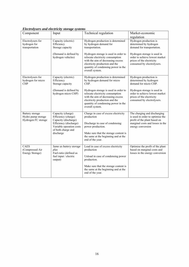
Electrolysers and electricity storage systems Component Input Technical regulation Market-economic

regulation Electrolysers for hydrogen for transportation

Capacity (electric) Efficiency Storage capacity (Demand is defined by hydrogen vehicles)

Hydrogen production is determined by hydrogen demand for transportation. Hydrogen storage is used in order to relocate electricity consumption with the aim of decreasing excess electricity production and the quantity of condensing power in the overall system.

Hydrogen production is determined by hydrogen demand for transportation. Hydrogen storage is used in order to achieve lowest market prices of the electricity consumed by electrolysers.

Electrolysers for hydrogen for micro CHP

Capacity (electric) Efficiency Storage capacity (Demand is defined by hydrogen micro CHP)

Hydrogen production is determined by hydrogen demand for micro CHP. Hydrogen storage is used in order to relocate electricity consumption with the aim of decreasing excess electricity production and the quantity of condensing power in the overall system.

Hydrogen production is determined by hydrogen demand for micro CHP. Hydrogen storage is used in order to achieve lowest market prices of the electricity consumed by electrolysers.

Battery storage Hydro pump storage Hydrogen FC storage

Capacity (charge) Efficiency (charge) Capacity (discharge) Efficiency (discharge) Variable operation costs of both charge and discharge

Charge in case of excess electricity production Discharge in case of condensing power production. Make sure that the storage content is the same at the beginning and at the end of the year.

The charging and discharging is used in order to optimise the profit of the plant based on marginal costs and losses in the energy conversion

CAES (Compressed Air Energy Storage)

Same as battery storage plus Fuel-ratio (defined as fuel input / electric output)

Load in case of excess electricity production Unload in case of condensing power production. Make sure that the storage content is the same at the beginning and at the end of the year.

Optimise the profit of the plant based on marginal costs and losses in the energy conversion

17

3. Libraries and settings The model is organised as an executable file and three libraries: Data, Distributions and Cost.

The Data Library holds input data set and the Distribution Library contains hour distributions files. The Cost Library includes data sets of investment and fuel costs. The Cost data is part of the input data set. However the Cost data allows for a quick shift or replacement of investment and fuel cost data without changing al the rest of the input. When ever one chose to save or load “input data” al input data including costs data will be handled. However, when one chose to save or load “cost data” only investment and fuel cost data are included. 3.1 Input data set The EnergyPLAN model always holds sufficient input data for doing a calculation. Moreover, the model controls if new input data meets the standards. If not they will be rejected. When the program is started the model automatically defines a set of input data, called “Startdata”. The input data set can be saved and stored in the Data Library. Stored data sets can be read into the model. In the upper left corner, the model shows the name of the present data set (see below).

3.1.1 Open an input data set from the Library To open an input data set from the Library, activate the open button in the upper left corner.

18

The following window will open, in which one can choose between stored input data sets:

3.1.2 Defining a new input data set and storing it in the Library To define a new input data name and save present input data in the Library, activate the file button in the upper left corner and choose “Save As”:

The following window will open, in which one can define the name of the data set, e.g. “Example”:

19

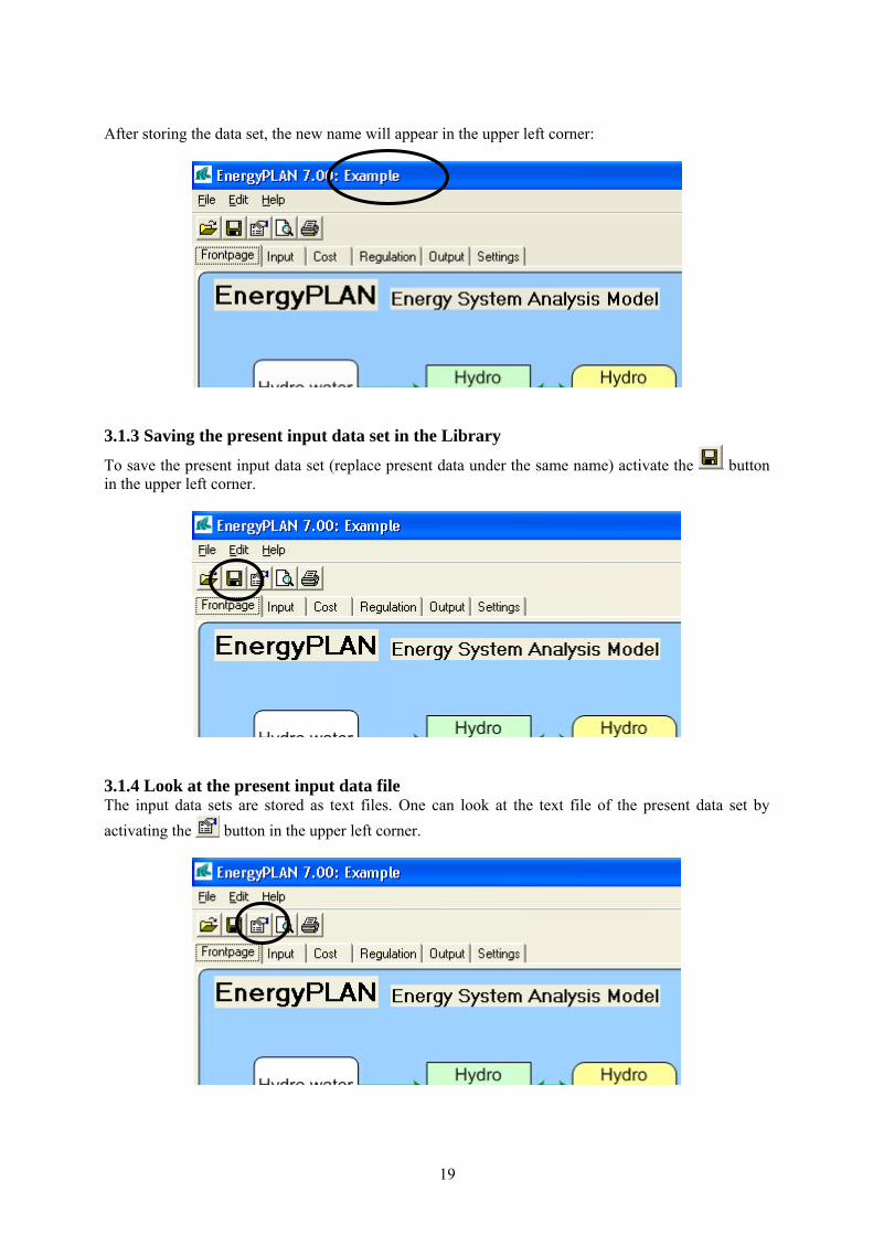
After storing the data set, the new name will appear in the upper left corner:

3.1.3 Saving the present input data set in the Library

To save the present input data set (replace present data under the same name) activate the button in the upper left corner.

3.1.4 Look at the present input data file The input data sets are stored as text files. One can look at the text file of the present data set by activating the button in the upper left corner.

20

3.2 Distribution Typically, energy demands and renewable resources etc. are defined in the model by an annual value and a distribution name from the Distribution Library. Distributions in the Library are stored as text files and consist of 8784 hour values presented on 8784 lines. New distributions have to meet this format. For price distributions, the 8784 numbers are absolute. For demands, all values are relative and will relate to the specified annual value. For renewable energy sources, distribution is relative to the specified capacities. Distributions are defined by their name, and such names are part of the input data set. When the model is started, names are defined for all distributions. However, one can easily change from one distribution to another in the Library. 3.2.1 Change distribution The model shows the name of the present distribution. Here illustrated by the electricity demand:

To change distribution, simply activate the button and the following window will open:

21

Here one can choose a new distribution, which will then be shown in the input window:

3.2.2 Define new distributions New distribution data can be added to the Library, simply by producing a text file with 8784 numbers. Distributions in the Library are stored as text files and consist of 8784 hourly values presented on 8784 lines. New distributions have to meet this format. One fast way of making a new distribution is to open an existing file in the Distribution Library by using the pathfinder. Then, change the data and save under a new name. One can mark all data and load the data into e.g. Excel and change them. Or one can simply replace them with a new set of data.

22

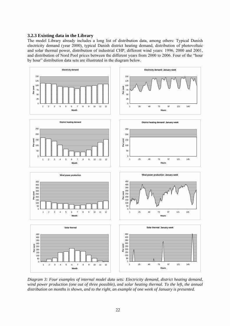
3.2.3 Existing data in the Library The model Library already includes a long list of distribution data, among others: Typical Danish electricity demand (year 2000), typical Danish district heating demand, distribution of photovoltaic and solar thermal power, distribution of industrial CHP, different wind years: 1996, 2000 and 2001, and distribution of Nord Pool prices between the different years from 2000 to 2006. Four of the “hour by hour” distribution data sets are illustrated in the diagram below.

Electricity demand

0

25

50

75

100

125

150

1 2 3 4 5 6 7 8 9 10 11 12

Month

Per c

ent

Electricity demand: January week

0

25

50

75

100

125

150

1 25 49 73 97 121 145

Hours

Per c

ent

District heating demand

0

50

100

150

200

250

1 2 3 4 5 6 7 8 9 10 11 12

Month

Per c

ent

District heating demand: January week

0

50

100

150

200

250

1 25 49 73 97 121 145

Hours

Per c

ent

Wind power production

050

100150200250300350400450

1 2 3 4 5 6 7 8 9 10 11 12

Month

Per c

ent

Wind power production: January week

050

100150200250300350400450

1 25 49 73 97 121 145

Hours

Per c

ent

Solar thermal

050

100150200250300350400450

1 2 3 4 5 6 7 8 9 10 11 12

Month

Per c

ent

Solar thermal: January week

050

100150200250300350400450

1 25 49 73 97 121 145

Hours

Per c

ent

Diagram 3: Four examples of internal model data sets: Electricity demand, district heating demand, wind power production (one out of three possible), and solar heating thermal. To the left, the annual distribution on months is shown, and to the right, an example of one week of January is presented.

23

3.3 Cost database To save or load Cost Data one has to go to the Cost Additional Tab-sheet and activate one of the two buttons “Save Cost Data” or “Load New Cost Data”.

When activating one of these buttons the following picture will show and one can either read new data or load present data in the same way as for input data.

24

3.4 Settings

In the settings window, one can define the energy units and monetary units. The unit is changed by activating one of the buttons “Change Unit”. Note: No input or output numbers will be changed by activating the button. Only the writing of units in the windows and on the printed pages is changed. The energy/capacity units can be changed by selecting between the following combinations:

- kW and GWh/year - MW and TWh/year - GW and PWh/year

25

4. Energy System Definition (Inputs)

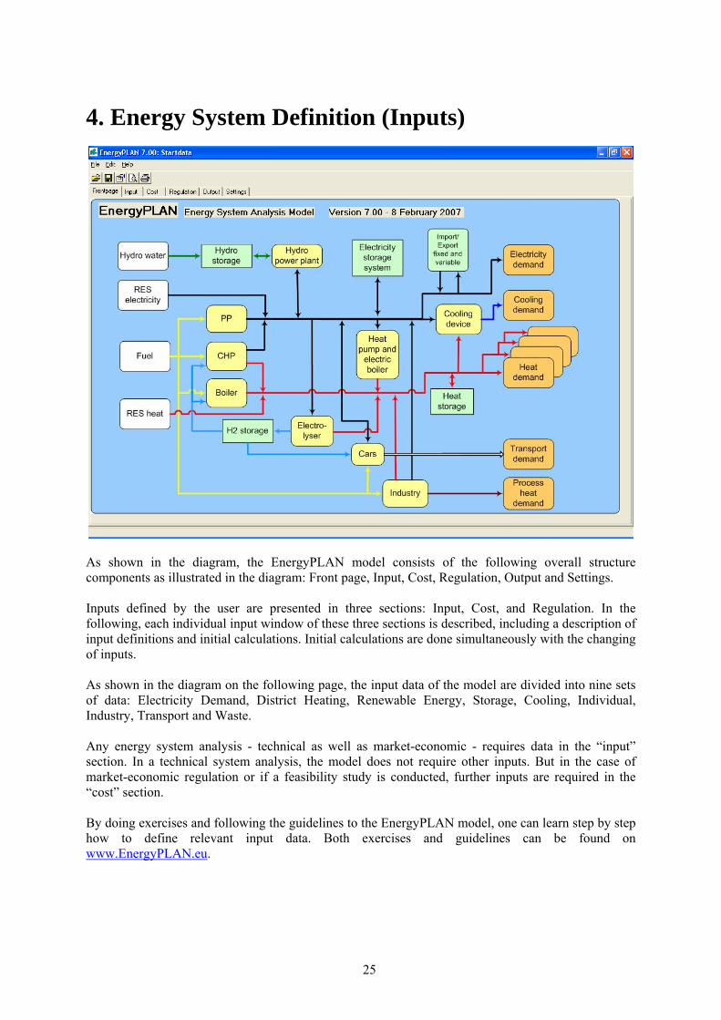
As shown in the diagram, the EnergyPLAN model consists of the following overall structure components as illustrated in the diagram: Front page, Input, Cost, Regulation, Output and Settings. Inputs defined by the user are presented in three sections: Input, Cost, and Regulation. In the following, each individual input window of these three sections is described, including a description of input definitions and initial calculations. Initial calculations are done simultaneously with the changing of inputs. As shown in the diagram on the following page, the input data of the model are divided into nine sets of data: Electricity Demand, District Heating, Renewable Energy, Storage, Cooling, Individual, Industry, Transport and Waste. Any energy system analysis - technical as well as market-economic - requires data in the “input” section. In a technical system analysis, the model does not require other inputs. But in the case of market-economic regulation or if a feasibility study is conducted, further inputs are required in the “cost” section. By doing exercises and following the guidelines to the EnergyPLAN model, one can learn step by step how to define relevant input data. Both exercises and guidelines can be found on www.EnergyPLAN.eu.

26

4.1 Electricity Demand

Inputs DE = Annual electricity demand DEH = Annual electricity demand for cooling (defined in the input window “Cooling”) DEC = Annual electricity demand for heating (defined in the input window “Individual”) DEX = Annual electricity demand of fixed exchange (Fixed import/export) DFXDay = Annual electricity demand flexible within 1 day DFXWeek = Annual electricity demand flexible within 1 week DFX4WeeK = Annual electricity demand flexible within 4 weeks CFXDay = Max capacity of 1-day flexible demand CFXWeek = Max capacity of 1-week flexible demand CFX4Week = Max capacity of 4-week flexible demand

The electricity demand is defined by an annual value, DE (TWh per year) and a name of an hour by hour distribution data set. And one can also specify a fixed import/export, DEX. Furthermore, one can define various kinds of flexible electricity demands, DFXDay, DFXWeek and DFX4Week in combination with maximum capacity values. Electricity demands for electric heating and cooling (specified in the “cooling” and the “individual” windows) are shown, and help functions make is possible to subtract such demands from the electricity demand. 4.1.1 Input window calculation of electricity demand If the electricity demand contains an electric heating or cooling demand, such demand (DEH and DEC) can be defined and will be subtracted from the electricity demand hour by hour:

dE’ = dE – dEH - dEC

if dE’ < 0 then dE’ = 0

DE’ = Σ dE’ If such electric heating or cooling demands are specified the new electricity demand, DE’ ,will be used afterwards as input to the energy system analysis.

27

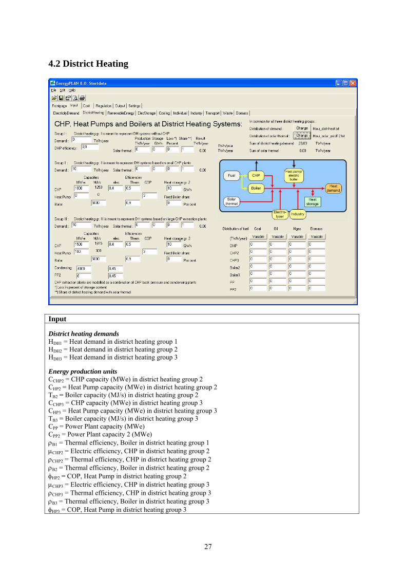
4.2 District Heating

Input District heating demands HDH1 = Heat demand in district heating group 1 HDH2 = Heat demand in district heating group 2 HDH3 = Heat demand in district heating group 3 Energy production units CCHP2 = CHP capacity (MWe) in district heating group 2 CHP2 = Heat Pump capacity (MWe) in district heating group 2 TB2 = Boiler capacity (MJ/s) in district heating group 2 CCHP3 = CHP capacity (MWe) in district heating group 3 CHP3 = Heat Pump capacity (MWe) in district heating group 3 TB3 = Boiler capacity (MJ/s) in district heating group 3 CPP = Power Plant capacity (MWe) CPP2 = Power Plant capacity 2 (MWe) ρB1 = Thermal efficiency, Boiler in district heating group 1 μCHP2 = Electric efficiency, CHP in district heating group 2 ρCHP2 = Thermal efficiency, CHP in district heating group 2 ρB2 = Thermal efficiency, Boiler in district heating group 2 φHP2 = COP, Heat Pump in district heating group 2 μCHP3 = Electric efficiency, CHP in district heating group 3 ρCHP3 = Thermal efficiency, CHP in district heating group 3 ρB3 = Thermal efficiency, Boiler in district heating group 3 φHP3 = COP, Heat Pump in district heating group 3

28

μPP = Electric efficiency, Power Plant μPP2 = Electric efficiency, Power Plant 2 Heat storage SDH2 = Capacity, Heat storage in district heating group 2 (GWh) SDH3 = Capacity, Heat storage in district heating group 3 (GWh) SHSsolar1 = Capacity, Heat storage for solar thermal in district heating group 1 (GWh) SHSsolar2 = Capacity, Heat storage for solar thermal in district heating group 2 (GWh) SHSsolar3 = Capacity, Heat storage for solar thermal in district heating group 3 (GWh) LOSSHSsolar1, ….LOSSHSsolar3 = Losses in Heat storage for solar thermal in district heating groups 1, 2 and 3. Solar thermal QSolar1, ….QSolar3 = Annual heat production from solar thermal in district heating groups 1, 2 and 3. SHARESolar1, …. SHARESolar3 = Share of district heating with solar thermal in groups 1, 2 and 3. The annual district heating consumption must be stated for each of the three DH groups. The annual solar thermal production is also defined for each group and includes heat storage capacity and losses. The share of solar is a figure between 0 and 1 defining the share of district heating demand with solar thermal production. For both district heating and solar thermal production, a common hour distribution for all three groups is specified. Capacities and operation efficiencies of CHP units, power stations, boilers and heat pumps are defined as part of the input data. And also the size of heat storage capacities is given here. CPP is the total sum of power plant capacity and CHP capacity in group 3. In lack of district heating demand in group 3, the CHP capacity can be turned into purely condensing power plant capacity. And often CHP plants in city areas are part of extraction plants. 4.2.1 Input window calculation of solar thermal in district heating systems The solar thermal input can not always be utilised. It depends on the hour distributions of the heat demand, the solar thermal production, the heat storage and the losses. The share of the solar thermal production, which can be utilised, Q´Solar, is calculated simultaneously in the input window for each of the three district heating groups. If the solar production at one hour exceeds the demand, the excess production is stored (if possible). And when the solar production is lower than the demand, the model seeks to empty the storage:

q’DH = qDH * SHARESolar

If qSolar < q’DH then q’Solar = qSolar + Min[StorageContent, (q’DH – qSolar)]

If qSolar > q’DH then q’Solar = q’DH + (SHSsolar - StorageContent)

StorageContent := StorageContent + qSolar – q’DH

If StorageContent > SHSsolar then StorageContent = SHSsolar

StorageContent:=StorageContent- StorageContent * LOSSHSsolar1 /100;

Q´Solar = Σ q´solar Q´Solar is shown in the input window for each of the three groups, and q´Solar is applied subsequently to the energy system analysis.

29

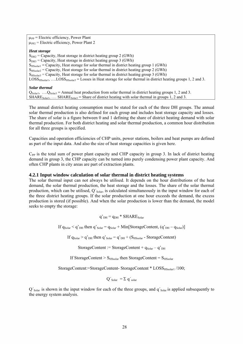
4.3 Renewable Energy Sources (RES)

Input Renewable Energy Sources CRes1, ....CRes4 = Annual electricity production from Renewable Energy Resources StabRes1, ….StabRes4 = Share of RES capacity with grid stabilisation capabilities FACRes1, ….FACRes4 = Correction factor of RES production Hydro power CHydro = Capacity of Electricity Generator in MW μHydro = Efficiency defined as the conversion from energy in the storage into electricity production. SHydro = Capacity of the storage in GWh WHydro = Annual water supply to the storage in TWh/year CHydro-Pump = Capacity of the Hydro Power Pump in MW αHydro-Pump = Efficiency of Pump defined as the conversion from electricity to energy in the storage SHydro-Pump = Capacity of the lower water storage in GWh Nuclear or Geothermal CNuclear = Capacity of the Nuclear Power Electricity Generator in MW μNuclear = Efficiency of the Nuclear Power station. The input data set defines input from RES and nuclear power. One can choose inputs from up to four different renewable energy sources. By pressing the button, the following specification can be attached to each RES:

- Wind

30

- Offshore Wind - Photo Voltaic - Wave Power - River Hydro

Input to the electricity production is identified by the capacity of each RES and the by the name of the distribution file. In the case that the RES contributes to grid stabilisation, a share between 0 and 1 can be given. Furthermore, one can specify hydro power input including reversal hydro power and either nuclear power or geothermal power. 4.3.1 Input window calculation of RES electricity production The electricity production input from intermittent renewable energy sources such as e.g. wind power is found by multiplying the capacity by the specified hour by hour distribution. The Data Library comprises different distributions typically found from historical data. The resulting annual production based on the specified input capacity and distribution is shown on the input page. However, different future wind turbine configurations would lead to either lower or higher productions in the same wind years. Therefore, one can choose to specify a correction factor to change the distribution and increase the annual production. The factor changes the production in such a way that the productions remain the same at hours with either no production or full production, while the other values are moderated relatively:

eRes’ = eRes * 1 / [1 – FACRes * (1 – eRes)] The same procedure is used for the possible modification of any of the renewable sources. In the following diagrams, it is illustrated how the factor modifies the input. The examples are based on wind power and photovoltaic distributions in the area of western Denmark year 2001. When defining a capacity of 1000 MW wind power, the annual production becomes 1.96 TWh/year, and when defining 1000 MW of photovoltaic power, the annual production becomes 1.00 TWh/year, as shown in rows 1 and 3 in the input window below.

31

If adding a correction factor of e.g. 0.8, the hour by hour production is modified as illustrated in the two following diagrams. The 0 values and the maximum values of 1000 MW are kept, while all the values in between those are raised in accordance with the formula described above. As a result, annual productions are raised to 4.10 TWh/year for wind power and 2.02 TWh/year for photovoltaic power. It should be mentioned that the factor 0.8 is very high especially for photovoltaic power. However, such a high factor is suitable for the illustration of the principle of modifications.

Wind Power in Jutland 2001

0200400600800

1000

6893 6943 6993 7043 7093 7143 7193 7243

hours

MW

Factor 0 Factor 0.8

Photo Voltaic in Jutland 2001

0200400600800

1000

3000 3050 3100

hours

MW

Factor 0 Factor 0.8

4.3.2 Input window calculation of hydro power The hydro power plant is identified by an hourly distribution of the annual water input (WHydro), a water storage capacity (SHydro) and the capacity (CHydro) and efficiency (μHydro) of the generator. Based on such input, the potential output is calculated simultaneously by the procedure described in the following. First, the average hydro electricity production (eHydro-ave) is calculated as the output of the average water supply (Annual water supply divided by 8784 hours/year):

32

eHydro-ave = μHydro * WHydro / 8784

Then the program calculates the hour by hour modelling of the system, including the fluctuations in the storage content. Furthermore, the hydro power production (eHydro) is modified in accordance with the generator capacity, the distribution of the water supply, and the storage capacity in the following way:

Hydro-storage-content = Hydro-storage content + wHydro

eHydro = MAX [eHydro-Ave , (Hydro-storage-content - SHydro)* μHydro]

eHydro <= CHydro Due to differences in the storage content at the beginning and at the end of the calculation period errors may appear in the calculations. To correct these, the above calculation seeks to identify a solution in which the storage content at the end is the same as at the beginning. Initially, the storage content is defined as 50% of the storage capacity. After the first calculation, a new initial content is defined as the resulting content at the end of the former calculation. The annual potential production of the hydro power plant is calculated and shown in the input window. 4.3.3 Input window calculation of nuclear power or geothermal power. By activating the button with the name, one can choose to include either nuclear power or geothermal power in the input. Both types of power production are calculated the same way, here described for the nuclear power plants. Nuclear power units are determined by the following inputs: CNuclear = Capacity of the nuclear power electricity generator in MW μNuclear = Efficiency of the nuclear power station. dNuclear = Distribution of the electricity production between 8784 hour values The nuclear power station is subject to the condition that it will always be involved in the task of maintaining grid stability. The nuclear unit is considered to be running as base load, and therefore the power plant does not take part in the active regulation. The electricity production of the nuclear unit (eNuclear) is simply defined by the capacity and the hour by hour distribution:

eNuclear = CNuclear * dNuclear / Max(dNuclear) The efficiency is used only for the calculation of the annual amount of fuel (fNUCLEAR) which is calculated by applying the following formula:

fNuclear = eNuclear / μNuclear The fuel consumption is named “Uranium” and is measured in TWh/year in order to be able to compare it to the consumption of the rest of the units. In the case of geothermal, the fuel is named “Geothermal”.

33

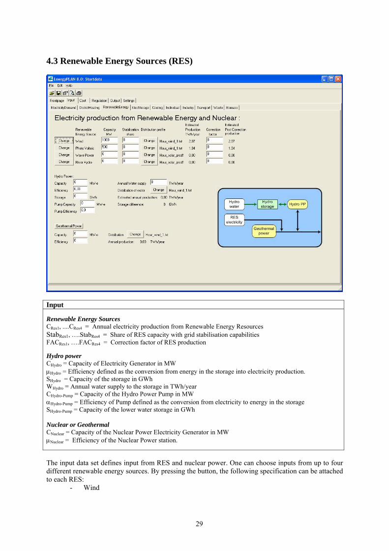
4.4 ElecStorage

Input Electrolysers CElc2 = Capacity of Electrolysers in district heating group 2 CElc3 = Capacity of Electrolysers in district heating group 3 CElcT = Capacity of Electrolysers for Transportation CElcM = Capacity of Electrolysers for Micro CHP αElc2 = Fuel efficiency of Electrolysers in district heating group 2 αElc3 = Fuel efficiency of Electrolysers in district heating group 3 αElcT = Fuel efficiency of Electrolysers for Transportation αElcM = Fuel efficiency of Electrolysers for Micro CHP ρElc2 = Thermal efficiency of Electrolysers in district heating group 2 ρElc3 = Thermal efficiency of Electrolysers in district heating group 3 SElc2 = Capacity of Electrolysers Fuel Storage in district heating group 2 SElc3 = Capacity of Electrolysers Fuel Storage in district heating group 3 SElcT = Capacity of Electrolysers Fuel Storage, Transportation SElcM = Capacity of Electrolysers Fuel Storage, Micro CHP Electricity Storage CPump = Capacity of Pump in electricity storage CTurbine = Capacity of Turbine in electricity storage SCAES = Capacity of Storage, electricity storage system αPump = Efficiency of Pump in electricity storage (from electricity to storage input) μTurbine = Efficiency of Turbine in electricity storage (from storage output to electricity) φCAES = Fuel-ration for CAES systems (fuel input / electric output) In the storage input window, one can specify electrolyser and electricity storage systems. The two first electrolysers are described in the model as located in either district heating group 2 or group 3 along with the CHP units, Heat Pumps and boilers. The two next electrolysers are used for hydrogen

34

production for transportation or micro CHP. The electrolysers transform electricity into fuel and heat if located in connection to district heating. They are defined by a capacity, a fuel efficiency and a thermal efficiency. Moreover, fuel storage is defined by a capacity. The electricity storage can represent e.g. hydro pump storage, a battery or a FC/electrolyser hydrogen storage and is represented by the following inputs:

• Pump (converting electricity to potential energy) defined by a capacity and an efficiency • Turbine (converting potential energy to electricity) defined by a capacity and an efficiency • Storage (storing energy) defined by a capacity.

Also the model can add fuel when the turbine is activated and thereby technologies such as CAES (Compressed Air Energy Storage) can be modelled. In such case, the following input has to be defined:

• CAES fuel ratio defined as CAES fuel consumption / electric output.

35

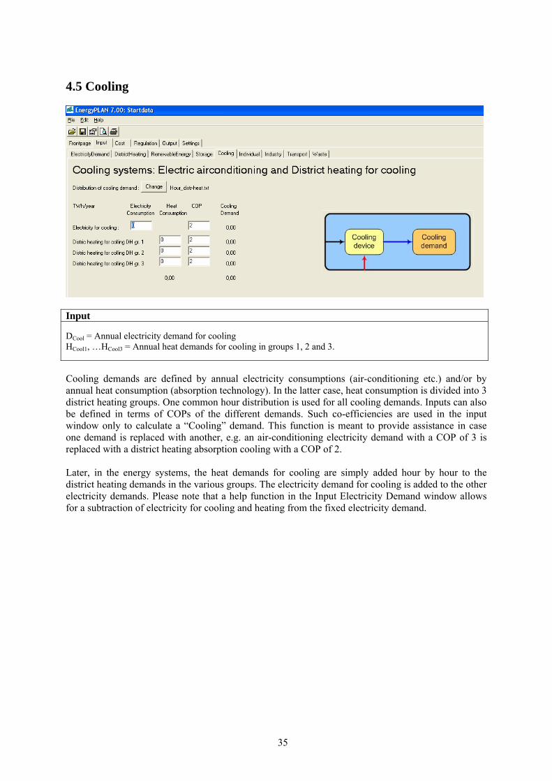
4.5 Cooling

Input DCool = Annual electricity demand for cooling HCool1, …HCool3 = Annual heat demands for cooling in groups 1, 2 and 3. Cooling demands are defined by annual electricity consumptions (air-conditioning etc.) and/or by annual heat consumption (absorption technology). In the latter case, heat consumption is divided into 3 district heating groups. One common hour distribution is used for all cooling demands. Inputs can also be defined in terms of COPs of the different demands. Such co-efficiencies are used in the input window only to calculate a “Cooling” demand. This function is meant to provide assistance in case one demand is replaced with another, e.g. an air-conditioning electricity demand with a COP of 3 is replaced with a district heating absorption cooling with a COP of 2. Later, in the energy systems, the heat demands for cooling are simply added hour by hour to the district heating demands in the various groups. The electricity demand for cooling is added to the other electricity demands. Please note that a help function in the Input Electricity Demand window allows for a subtraction of electricity for cooling and heating from the fixed electricity demand.

36

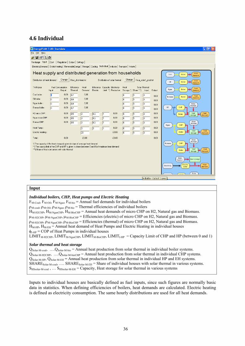
4.6 Individual

Input Individual boilers, CHP, Heat pumps and Electric Heating FM-Coal, FM-Oil, FM-Ngas, FM-bio = Annual fuel demands for individual boilers ρM-coal, ρM-Oil, ρM-Ngas, ρM-bio = Thermal efficiencies of individual boilers HM-H2CHP, HM-NgasCHP, HM-BioCHP = Annual heat demands of micro CHP on H2, Natural gas and Biomass. μM-H2CHP, μM-NgasCHP, μM-BioCHP = Efficiencies (electric) of micro CHP on H2, Natural gas and Biomass. ρM-H2CHP, ρM-NgasCHP, ρM-BioCHP = Efficiencies (thermal) of micro CHP on H2, Natural gas and Biomass. HM-HP, HM-EH = Annual heat demand of Heat Pumps and Electric Heating in individual houses φI-HP = COP of Heat Pumps in individual houses LIMITM-H2CHP, LIMITM-NgasCHP, LIMITM-BioCHP, LIMITI-HP = Capacity Limit of CHP and HP (between 0 and 1) Solar thermal and heat storage QSolar-M-coal, ….QSolar-M-bio = Annual heat production from solar thermal in individual boiler systems. QSolar-M-H2CHP, ….QSolar-M-bioCHP = Annual heat production from solar thermal in individual CHP systems. QSolar-M-HP, QSolar-M-EH = Annual heat production from solar thermal in individual HP and EH systems. SHARESolar-M-coal, …. SHARESolar-M-EH = Share of individual houses with solar thermal in various systems. SHSsolar-M-coal , … SHSsolar-M-EH = Capacity, Heat storage for solar thermal in various systems Inputs to individual houses are basically defined as fuel inputs, since such figures are normally basic data in statistics. When defining efficiencies of boilers, heat demands are calculated. Electric heating is defined as electricity consumption. The same hourly distributions are used for all heat demands.

37

To include CHP and Heat Pumps one has to define heat demands and efficiencies. Moreover, one can define capacity limits in the CHP and Heat Pump units in shares of the maximum heating demand (figures between 0 and 1). If such limits are defined, the peak heat demands will be met by boilers using the same efficiencies as defined for the boiler-only systems. In the case of H2, the efficiency of the natural gas boiler is used; and in the case of Heat Pumps, electric heating is used. Moreover, one can add solar thermal power to all the systems by defining the annual solar production and the share of heat demand based on solar thermal power. For all solar thermal productions, the same hourly distributions are used. The following are calculated on a simultaneous basis in the input window: 4.6.1 Input window calculation of heat demands in individual houses The resulting heat demands in the individual houses are given as input to the micro CHP and Heat Pump systems. For the boiler-only systems, the heat demands are calculated simply as the fuel input multiplied by the boiler efficiencies:

H = F / ρ 4.6.2 Input window calculation of solar thermal production in individual houses Solar production is calculated principally in the same way as solar thermal production in district heating. If the solar production at one hour exceeds the demand, the excess production is stored if possible, and if not, the excess production is perceived as waste. When the solar production is lower than the demand the model seeks to empty the storage. The same calculation methodology is used as in section 4.2.1. 4.6.3 Input window calculation of boilers, CHP and heat pumps in individual houses The heat demand for solar production is supplied by boilers, micro CHPs and heat pumps. The production in the boilers-only systems is simply calculated as the difference between the demand and the solar production (including the use of the heat storage):

qM-Oil = hM-Oil – q’Solar-M-Oil For the micro CHP and the Heat Pump the production cannot exceed the limitations in capacity if any.

qM-NgasCHP = hM-NgasCHP – q’Solar-M-NgasCHP

If qM-NgasCHP > Max(hM-NgasCHP) * LIMITM-NgasCHP then qM-NgasCHP = Max(hM-NgasCHP) * LIMITM-NgasCHP The heat demand remaining after coverage by solar (including the use of storage), CHP and Heat Pumps is met by boilers and in the case of heat pumps by electric heating:

qM-H2CHP-Boiler = hM-H2CHP - q’Solar-M-H2CHP - qM-H2CHP

qM-NgasCHP-Boiler = hM-NgasCHP - q’Solar-M-NgasCHP - qM-NgasCHP

qM-BioCHP-Boiler = hM-BioCHP - q’Solar-M-BioCHP - qM-BioCHP

qM-HP-EH = hM-HP - q’Solar-M-HP - qM-HP The fuel demands for all boiler systems are calculated and shown in the input window (Here shown for the oil boiler):

38

fM-Oil = qM-Oil / ρM-Oil The fuel demands for the three CHP systems (here shown for the Ngas system) are calculated individually for the CHP unit and the peak load boiler.

fM-NgasCHP = qM-NgasCHP / ρM-NgasCHP

fM-NgasCHP-Boiler = qM-NgasCHP-Boiler / ρM-Ngas The total fuel demand, FM-NgasCHP-Total, is found by adding the two demands:

fM-NgasCHP-Total = fM-NgasCHP-Boiler + fM-NgasCHP The electricity production from CHP is calculated as follows:

eM-NgasCHP = fM-NgasCHP * μM-NgasCHP The total electricity consumption from Heat Pumps, DI-HP-Total, is calculated as follows:

dM-HP-EH = qM-HP-EH

dM-HP = qM-HP / φM-HP

dM-HP-total = dM-HP-EH + dM-HP The electricity demand for electric heating is calculated like this:

DM-EH = qM-EH The resulting total fuel consumption and electricity productions (and consumptions) are shown in the input window for all systems. So is the resulting solar production. 4.6.4 Input window calculation of Electrolysers for micro H2 CHP systems If a heat demand is specified for the micro H2 CHP system, then the minimum electrolyser capacity required to provide the necessary hydrogen is calculated. The electrolysers must be added to the system in the Input Storage window. If hydrogen storage is specified in the Input Storage window, then such storage capacity is taken into account. The minimum electrolyser capacity, CELC-MIN, is calculated in the following way: First, the hydrogen production of the electrolyser fElcM is defined as the average hydrogen consumption of the micro CHP system, fM-H2CHP-Average :

fElcM = fM-H2CHP-Average = FM-H2CHP / 8784

Then for each hour x the hydrogen storage content is calculated, sElcM(x), as the content of the previous hour plus the average production minus the actual consumption of the hour.

sElcM(x) = sElcM(x-1) + fM-H2CHP-Average - fM-H2CHP (x)

If at one hour the storage content exceeds the capacity, the production is decreased:

39

If sElcM > SElcM then fElcM = fElcM - (sElcM - SElcM) And if the storage content goes below zero, the production is increased:

If sElcM < 0 then fElcM = fElcM - sElcM Due to differences in the storage content at the beginning and at the end of the calculation period, errors may appear in the calculation. To correct these errors the above calculation seeks to identify a solution in which the storage content at the end is the same as at the beginning. Initially, the storage content is defined as 50% of the storage capacity. After the first calculation, a new initial content is defined as the resulting content at the end of the former calculation. Finally, the minimum electrolyser capacity, CElc-MIN, is found as the maximum production needed divided by the fuel efficiency:

CElc-MIN = Hourmax( fElcM ) / αElcM

Also the corresponding electricity demand dElcM can be calculated:

dElcM = fElcM / αElcM The electricity demand dElcM forms the basis for the further calculation in section 6.7.1, in which the electrolysers are used for decreasing excess and power only production in the system.

40

4.7 Industry

Input FI-Coal, FI-Oil, FI-Ngas, FI-bio = Annual fuel demands for Industry FV-Coal, FV-Oil, FV-Ngas, FV-bio = Annual fuel demands for Various QI1, …. QI3 = Annual excess heat production from industry to district heating groups 1, 2 and 3. ECSHP1, …. ECSHP3 = Annual excess electricity production from industrial CHP (CSHP) Inputs to Industry are basically defined as fuel inputs, since such figures are normally basic data in statistics. Moreover, electricity and excess heat productions from industrial CHP or similar are defined, which are fed into one of the three district heating groups. Heat production for district heating groups is given priority along with solar thermal and heat production from waste as explained in section 5.5 (for group 1) and in sections 6.2.1 or 7.4 (for groups 2 and 3). Electricity production can be specified for each of the three district heating groups. However, they are all fed into the grid and given priority along with renewable energy resources such as wind power. Other units such as CHP and power plants will adjust their production accordingly if possible (given the specified regulation strategy), and if this can not be done, excess electricity production will be exported.

41

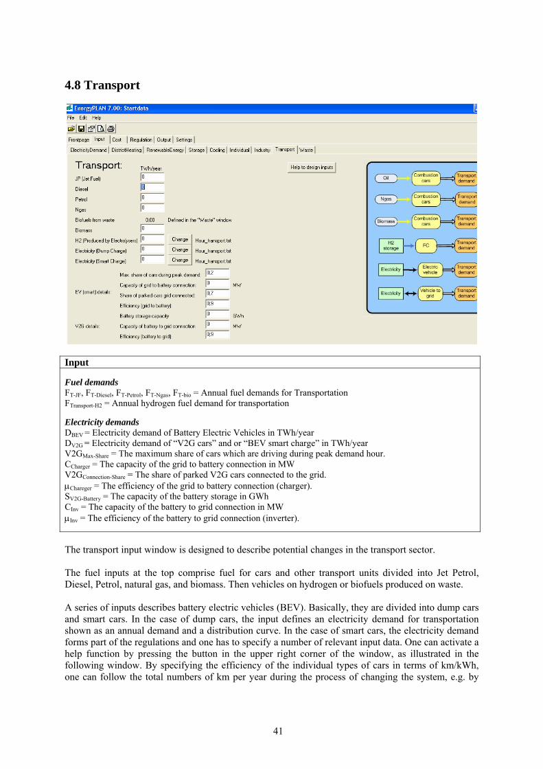
4.8 Transport

Input Fuel demands FT-JF, FT-Diesel, FT-Petrol, FT-Ngas, FT-bio = Annual fuel demands for Transportation FTransport-H2 = Annual hydrogen fuel demand for transportation Electricity demands DBEV = Electricity demand of Battery Electric Vehicles in TWh/year DV2G = Electricity demand of “V2G cars” and or “BEV smart charge” in TWh/year V2GMax-Share = The maximum share of cars which are driving during peak demand hour. CCharger = The capacity of the grid to battery connection in MW V2GConnection-Share = The share of parked V2G cars connected to the grid. μChareger = The efficiency of the grid to battery connection (charger). SV2G-Battery = The capacity of the battery storage in GWh CInv = The capacity of the battery to grid connection in MW μInv = The efficiency of the battery to grid connection (inverter). The transport input window is designed to describe potential changes in the transport sector. The fuel inputs at the top comprise fuel for cars and other transport units divided into Jet Petrol, Diesel, Petrol, natural gas, and biomass. Then vehicles on hydrogen or biofuels produced on waste. A series of inputs describes battery electric vehicles (BEV). Basically, they are divided into dump cars and smart cars. In the case of dump cars, the input defines an electricity demand for transportation shown as an annual demand and a distribution curve. In the case of smart cars, the electricity demand forms part of the regulations and one has to specify a number of relevant input data. One can activate a help function by pressing the button in the upper right corner of the window, as illustrated in the following window. By specifying the efficiency of the individual types of cars in terms of km/kWh, one can follow the total numbers of km per year during the process of changing the system, e.g. by

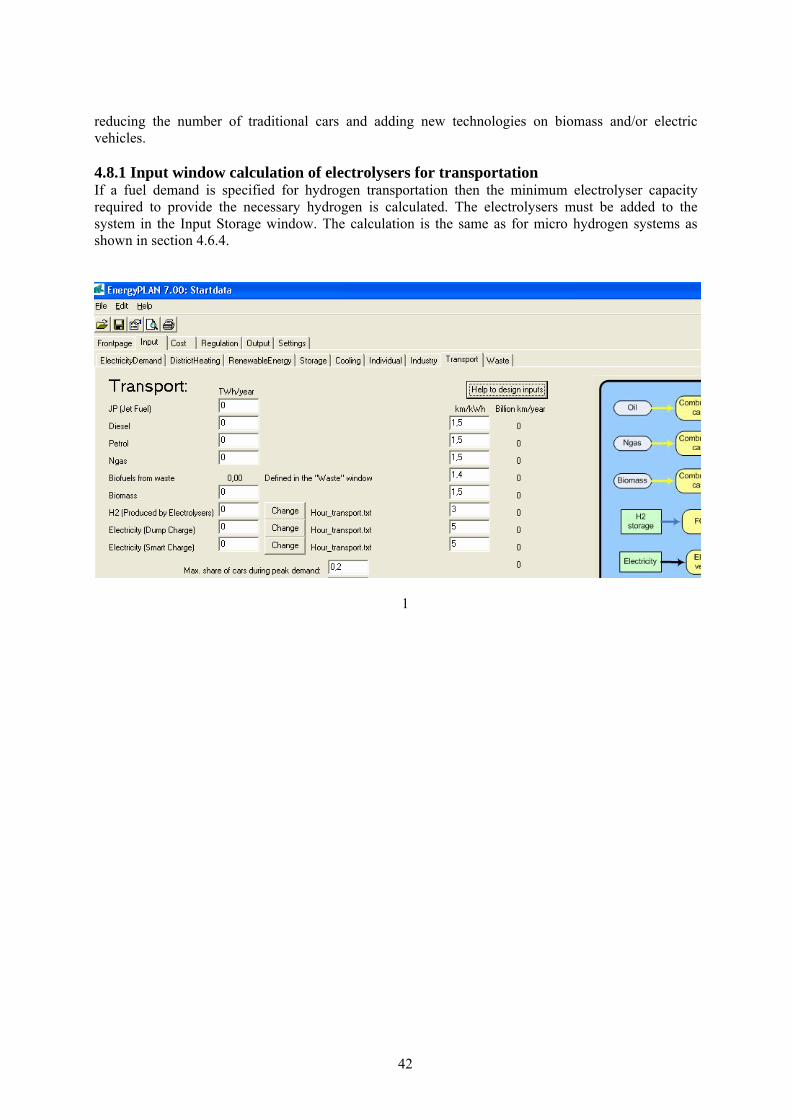
42

reducing the number of traditional cars and adding new technologies on biomass and/or electric vehicles. 4.8.1 Input window calculation of electrolysers for transportation If a fuel demand is specified for hydrogen transportation then the minimum electrolyser capacity required to provide the necessary hydrogen is calculated. The electrolysers must be added to the system in the Input Storage window. The calculation is the same as for micro hydrogen systems as shown in section 4.6.4.

1

43

4.9 Waste

Input FW1, FW2, FW3 = Annual input of waste fuels divided into the three district heating groups ρW1, ρW2, ρW3 = Efficiencies (thermal) of waste conversion μW1, μW2, μW3 = Efficiencies (electric) of waste conversion ψW1, ψW2, ψW3 = Efficiencies (waste to biofuel for transportation) of waste conversion ηW1, ηW2, ηW3 = Efficiencies (waste to biofuel for CHP and boilers) of waste conversion τW1, τW2, τW3 = Efficiencies (waste to various non energy products) of waste conversion PW1, PW2, PW3 = Prices of various non energy products (MDKK/TWh) ρW2-GEO, ρW3-GEO = Efficiencies (thermal) of waste conversion when also producing steam for geothermal HP μW2-GEO, μW3-GEO = Efficiencies (electric) of waste conversion when also producing steam for geothermal HP σW2-GEO, σW3-GEO = Efficiencies (steam) of waste conversion (Used geothermal HP) φGEO-Steam, φGEO-Steam = COP of geothermal HPs when provided with steam directly from Waste CHP φGEO-SteamStorage, φGEO-SteamStorage = COP of geothermal HPs when provided with steam from steam storgae SGEO2, SGEO3 = Steam Storage Capacities (GWh) LOSSGEO2, LOSSGEO3 = Energy Losses from Steam Storage in percent/hour (GWh) Waste is considered biomass energy, which can not be stored but has to be burned continuously. Waste is divided geographically into three district heating groups and only one hourly distribution can be defined. Waste can be converted into the following: - heat production, which is given priority in the three district heating groups

44

- electricity production which is being fed into the grid - biofuels (fluid) for transportation, which are transferred to the Input Transport window - biofuels (solid) for CHP and boilers, which are subtracted from the fuels in the respective DH

groups - Various (non energy) products which are given an economic value.

The following input must to be given to the model: - The waste resources divided geographically between the three district heating systems mentioned

above. - Efficiencies specifying the quantity of the waste input resources converted into the following 4

energy forms: Heat for district heating, electricity, fuel for transportation and fuel for CHP and boilers.

- An hour by hour distribution of the waste input (heat and electricity output) Moreover, one can specify an additional non energy output (such as animal food) which will then be given an economic value in the feasibility study.

Basically, the model assumes that waste can not be stored and has to be converted in accordance with the specified hour by hour input. Consequently, the energy outputs are treated in the following way: Heat production for district heating is given priority along with solar thermal and industrial waste heat production. If such input can not be utilized because of limitations in demand and heat storage capacity, the heat is simply wasted. Electricity production is fed into the grid and given priority along with renewable energy resources such as wind power. Other units such as CHP and power plants will adjust their production accordingly if possible (given the specified regulation strategy), and if this can not be done, excess electricity production will be exported. Fuel for transport is calculated and the used fuel can subtract the petrol accordingly and, at the same time, adjust for differences in car efficiencies if any. Fuel for CHP and boilers is automatically subtracted in the calculation of fuel in the relevant district heating groups.

Geothermal energy for District Heating in combination with Waste CHP One can specify a geothermal heat production operated by the use of an absorption heat pump fuelled by steam from the waste CHP plants in District Heating group 2 and 3. The option is defined by the following input data: - alternative electric, thermal and steam efficiencies of the Waste CHP plant - A COP of the absorption heat pump defined as the heat output divided by the steam input The waste CHP plant will still burn all the waste input in accordance with the specified hour be hour input. However the CHP plant can now be operated linear between the two operation modes with or without steam production and with the low or the high electricity and thermal outputs. Moreover one can specify the option of steam storage by defining a capacity and an energy loss if any. In regulation strategy 1 and 4 the system are operated in the following way: If the thermal output from the Waste CHP is exceeding the district heating demand and if it is possible to store steam, the CHP will decrease electricity and heat production and increase steam production accordingly, and the steam are stored. If the heat demand exceeds the thermal output from Waste CHP (and industrial waste heat and solar heating) the geothermal production will coved as much as possible only limited by the

45

capacity of the absorption heat pump and the heat demand. First, the absorption heat pump will use steam from the storage and thereafter steam from the Waste CHP obtained by decreasing electricity and heat productions. I regulation strategy 2 and 3 additionally to the above regulation the Waste CHP will decrease electricity production in the case of excess electricity productions in the system if the steam storage is available. 4.9.1 Calculation of waste fuel outputs The biofuel outputs are calculated in the following way and the fuel for transportation is transferred to the Transport window:

FT-Waste = FW1 * ψW1 + FW2 * ψW2 + FW3 * ψW3

46

4.10 Biomass

Input DBiogas = Annual electricity demand for cooling HBiogasDH1, …HBiogasDH3 = Annual district heating demands for biogas in groups 1, 2 and 3. FBiogas = Annual biogas production The annual electricity demand for biogas production is calculated hour by hour and added to the electricity Demand. The annual district heating demand is calculated hour by hour and added to the respective district heating groups. Both calculations are done by the use of the specified hourly distribution. In the present version 8.0 the biogas production is not used yet. However the model is prepared for future calculation of biogas storage etc.

47

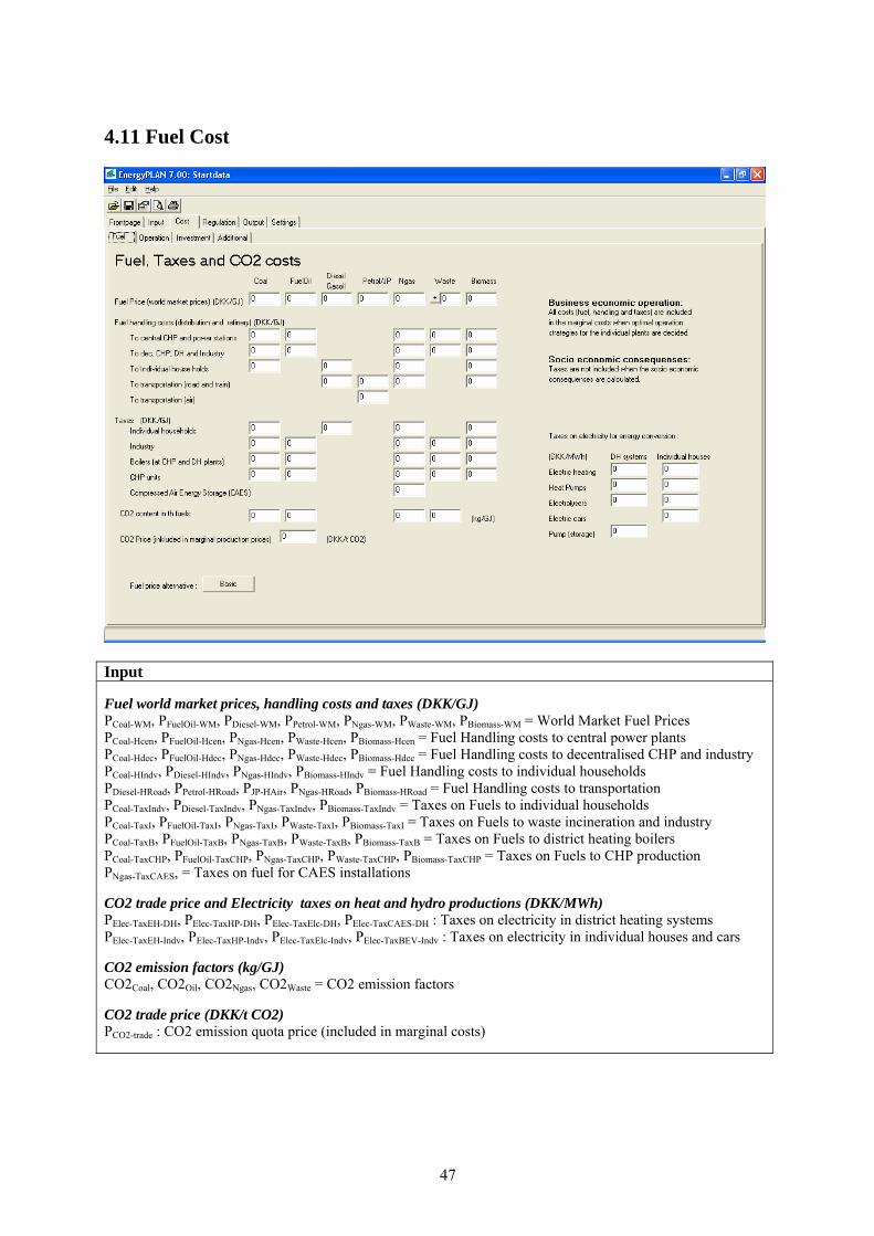
4.11 Fuel Cost

Input Fuel world market prices, handling costs and taxes (DKK/GJ) PCoal-WM, PFuelOil-WM, PDiesel-WM, PPetrol-WM, PNgas-WM, PWaste-WM, PBiomass-WM = World Market Fuel Prices PCoal-Hcen, PFuelOil-Hcen, PNgas-Hcen, PWaste-Hcen, PBiomass-Hcen = Fuel Handling costs to central power plants PCoal-Hdec, PFuelOil-Hdec, PNgas-Hdec, PWaste-Hdec, PBiomass-Hdec = Fuel Handling costs to decentralised CHP and industry PCoal-HIndv, PDiesel-HIndv, PNgas-HIndv, PBiomass-HIndv = Fuel Handling costs to individual households PDiesel-HRoad, PPetrol-HRoad, PJP-HAir, PNgas-HRoad, PBiomass-HRoad = Fuel Handling costs to transportation PCoal-TaxIndv, PDiesel-TaxIndv, PNgas-TaxIndv, PBiomass-TaxIndv = Taxes on Fuels to individual households PCoal-TaxI, PFuelOil-TaxI, PNgas-TaxI, PWaste-TaxI, PBiomass-TaxI = Taxes on Fuels to waste incineration and industry PCoal-TaxB, PFuelOil-TaxB, PNgas-TaxB, PWaste-TaxB, PBiomass-TaxB = Taxes on Fuels to district heating boilers PCoal-TaxCHP, PFuelOil-TaxCHP, PNgas-TaxCHP, PWaste-TaxCHP, PBiomass-TaxCHP = Taxes on Fuels to CHP production PNgas-TaxCAES, = Taxes on fuel for CAES installations CO2 trade price and Electricity taxes on heat and hydro productions (DKK/MWh) PElec-TaxEH-DH, PElec-TaxHP-DH, PElec-TaxElc-DH, PElec-TaxCAES-DH : Taxes on electricity in district heating systems PElec-TaxEH-Indv, PElec-TaxHP-Indv, PElec-TaxElc-Indv, PElec-TaxBEV-Indv : Taxes on electricity in individual houses and cars CO2 emission factors (kg/GJ) CO2Coal, CO2Oil, CO2Ngas, CO2Waste = CO2 emission factors CO2 trade price (DKK/t CO2) PCO2-trade : CO2 emission quota price (included in marginal costs)

48

The Fuel window is part of the Cost section. As shown in the diagram, the cost data of the model are divided into four sets of data: Fuel, Operation, Investment and Additional. The Additional window contains additional investment specification. An analysis using technical optimisation strategies can be done solely on technical data for the nine input windows described in the previous section. However, if one wants to include either market-economic optimisation or if a feasibility study is conducted, further inputs are required in the “cost” section. In the guidelines on how to use the EnergyPLAN model, one can learn how to conduct feasibility studies and market exchange studies when cost data input are provided for the model. Such analyses are conducted in exercise 5 and guidelines. Both can be found on www.EnergyPLAN.eu. Fuel prices are specified as world market prices and domestic handling costs and taxes, if any. The input in the Fuel Cost window is used for two purposes. The one is for the calculation of marginal productions costs, which is done in the Cost Operation window (see below in section 4.11). And the other is to include the fuel costs in the feasibility study at the end of the energy system analysis (see section 8.8)

49

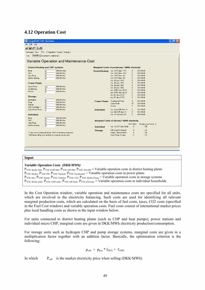
4.12 Operation Cost

Input Variable Operation Costs (DKK/MWh) PVOC-Boiler-DH, PVOC-CHP-DH, PVOC-HP-DH, PVOC-EH-DH = Variable operation costs in district heating plants PVOC-Hydro, PVOC-PP, PVOC-Nuclear, PVOC-Geothermal = Variable operation costs in power plants PVOC-Elc, PVOC-Pump, PVOC-Turbine, PVOC-V2G PVOC-Hydro-Pump = Variable operation costs in storage systems PVOC-Boiler-Indv, PVOC-CHP-Indv, PVOC-HP-Indv, PVOC-EH-Indv = Variable operation costs in individual households In the Cost Operation window, variable operation and maintenance costs are specified for all units, which are involved in the electricity balancing. Such costs are used for identifying all relevant marginal production costs, which are calculated on the basis of fuel costs, taxes, CO2 costs (specified in the Fuel Cost window) and variable operation costs. Fuel costs consist of international market prices plus local handling costs as shown in the input window below. For units connected to district heating plants (such as CHP and heat pumps), power stations and individual micro CHP, marginal costs are given in DKK/MWh electricity production/consumption.

For storage units such as hydrogen CHP and pump storage systems, marginal costs are given in a multiplication factor together with an addition factor. Basically, the optimisation criterion is the following:

psell > pbuy * fMUL + fADD In which Psell is the market electricity price when selling (DKK/MWh)

50

Pbuy is the market electricity price when buying (DKK/MWh) fMUL is the multiplication factor (always bigger than 1), and fADD is the addition factor (DKK/MWh)

The calculation of marginal production prices is based on the fuel specifications in the various input windows. Only fuels, which are specified as variable, are included in the calculation. 4.13 Investment Cost

Input For each component (here shown for wind): PUnit-Wind = Pr. unit price nWind = lifetime of investment PFOC-Wind = Fixed annual operation costs in percentage of total investment General for all calculations: i = calculation interest (real interest) for socio-economic evaluation In the Investment Cost window, the model summarises the input capacity specifications for the production units, and one can add unit prices, lifetimes and fixed operation and maintenance costs. Also one has to enter an interest for the whole calculation. The total investment, I, of each production unit is simply calculated as:

IWind = CWind * PUnit-Wind

51

The model then calculates the annual costs of each component divided into investment costs and fixed operation and maintenance costs. The annual costs, AInvestment, are calculated as follows:

AInvestment-Wind = IWind * i / [1 – (1+i)-n ] In which - IWind are the investment costs found by multiplying the number of units by the cost unit (MDKK

per unit). The unit is shown for each component. E.g. the unit for large CHP is MW, and consequently the cost is defined in million DKK/MW.

- n is the lifetime given in years. - i is the interest The annual fixed operation costs, AFOC, are calculated as follows:

AFOC-Wind = PFOC-Wind * IWind In which - PFOC is the annual fixed operation and maintenance costs given in percentage of the investment

cost.

52

4.14 Additional Cost

In the Additional Cost Tabsheet one can add and specify additional cost, i.e. investments that are not directly connected to the productions units such as insulation of buildings and transport infrastructure etc.

The additional costs are included in the calculation of total costs

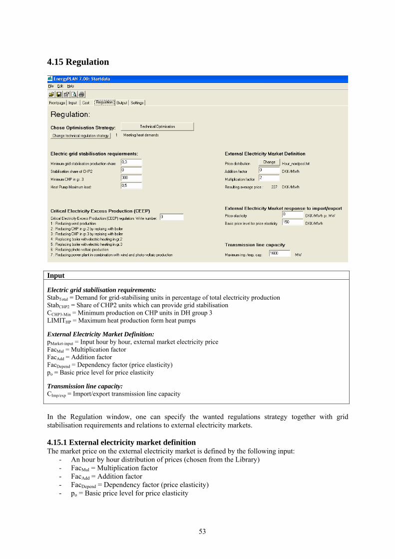
53

4.15 Regulation

Input Electric grid stabilisation requirements: StabTotal = Demand for grid-stabilising units in percentage of total electricity production StabCHP2 = Share of CHP2 units which can provide grid stabilisation CCHP3-Min = Minimum production on CHP units in DH group 3 LIMITHP = Maximum heat production form heat pumps External Electricity Market Definition: pMarket-input = Input hour by hour, external market electricity price FacMul = Multiplication factor FacAdd = Addition factor FacDepend = Dependency factor (price elasticity) po = Basic price level for price elasticity Transmission line capacity: CImp/exp = Import/export transmission line capacity In the Regulation window, one can specify the wanted regulations strategy together with grid stabilisation requirements and relations to external electricity markets. 4.15.1 External electricity market definition The market price on the external electricity market is defined by the following input:

- An hour by hour distribution of prices (chosen from the Library) - FacMul = Multiplication factor - FacAdd = Addition factor - FacDepend = Dependency factor (price elasticity) - po = Basic price level for price elasticity

54

For the economic optimisation, the market prices, pMarket, are found from the specified hour by hour price distribution (pMarket-input) when modified in the following way:

pMarket = pMarket-input * FacMul + FacAdd The resulting average market price after influence by the multiplication and addition factors is calculated simultaneously and shown in the window. In the economic optimisation strategy and in the calculation of income from exchange, the market price is further influenced by the price elasticity, as described in sections 7.1, 7.10 and 8.8.2. 4.15.2 Choice of regulations strategy The choice of regulation strategy is done by activating the upper button. Here, one can choose between Technical Optimisation, as described in chapter 6, or Market-Economic optimisation, as described in chapter 7.

If technical optimisation is selected, then one must choose between the following 4 technical optimisation strategies, all explained in chapter 6:

1. Balancing heat demands 2. Balancing both heat and electricity demands 3. Balancing both heat and electricity demands (Reducing CHP also when needed partly for grid

stabilisation) 4. Balancing heat demands using triple tariff

55

4.15.3 Choice of Critical Excess Electricity Production (CEEP) Regulation Strategy The electric connection to external electricity markets is limited by the definition of the capacity of the transmission lines. Based on such limitation, the model identifies Critical Excess Electricity Production (CEEP) as the export which exceeds the transmission line capacity. Such production is not allowed in real life, since this will cause a breakdown in the electricity supply. However, the model allows CEEP in order to be able to calculate the magnitude as a consequence of different regulation strategies, or one can ask the model to avoid CEEP. Seven options to remove critical excess electricity production can be activated:

1: Reducing RES1 and RES2 2: Reducing CHP production in group 2 (Replacing with boiler) 3: Reducing CHP production in group 3 (Replacing with boiler) 4: Replacing boiler production with electric heating in group 2. 5: Replacing boiler production with electric heating in group 3. 6: Reducing RES4 and RES5 7: Reducing power plant production in combination with RES1, RES2, RES3 and RES4

The seven possibilities are activated in a priority. If for instance "CEEP regulation" is stated as 23547, critical excess production will be removed first by replacing CHP in groups 2 and 3, then by electric heating and, in the end, by decreasing electricity production from RES1-RES4 together with power plants. For "CEEP regulation" = 51, excess production is removed first by increasing electric heating only in group 3 and then by stopping RES1 and RES2. All 7 options can be activated in all possible combinations. In chapter 8, it is explained how the reduction of CEEP is calculated and what the specific difference is between the options. 4.13.4 Grid Stabilisation Restrictions The model calculates hour by hour and basically assumes that all production units can change production from one hour to another. However, especially large steam turbine CHP or extraction plants have difficulties in going below a certain technical minimum, typically 20% of max capacity. Therefore, one can specify a minimum CHP3 production. Apart from such minimum production, one can specify limitations in the operation in order to assure grid stability. A certain percentage (30 percent is recommended) of the total electricity production must come from grid-stabilising units. CHP in group 3 and large power plants including hydro, geothermal and nuclear power are assumed to have such stabilising abilities. Therefore, one can specify to which extent small CHPs in group 2 and RES units can provide grid stabilisation.

56

5. Initial analyses not involving electricity balancing The model starts by making a number of initial calculations on the input data. Various electricity and heat demands are found simply by distributing the annual demands according to the internal hour by hour distributions. 5.1 Fixed import/export of electricity The fixed import/export demand is meant to describe exchanges with external electricity markets additional to the one, which is active in the model. Input is annual electricity demand, DEX, together with hourly distribution, δEX. The hour by hour values, dEX, are calculated as follows:

dEX = DEX * δEX / Σ δEX 5.2 District heating demands incl. heat demands from absorption cooling District heating demands in the three district heating groups, including the heating demand for biogas production and absorption cooling in the various groups are calculated in the following way. For all three district heating groups, the demand is defined by an annual heat demand, HDH, together with the hourly distribution, δDH. The same goes for heat demands for biogas production and absorption cooling in the various district heating groups: HCool and δCool. The hour by hour values, hDH, are calculated as follows:

hDH = HDH * δDH / Σ δDH + HCool * δCool / Σ δCool + HBiogasDH * δBiogasDH / Σ δBiogasDH 5.3 District heating and electricity productions from Industry and Waste District heating and electricity production from Industrial CHP are defined for each of the three district heating groups by the annual heat and electricity productions, QIndustry-DH and EIndustry-DH, together with the hourly distribution, δIndustry-DH.:

qIndustry-DH = QIndustry-DH * δIndustry-DH / Σ δIndustry-DH

eIndustry-DH = EIndustry-DH * δIndustry-DH / Σ δIndustry-DH District heating and electricity production from Waste are calculated in the same way:

qW = QW * δW / Σ δW

eW = EW * δW / Σ δW Both Industry and Waste are calculated separately for all three district heating groups. 5.4 Fixed Boiler production subtracted from the district heating demand The CHP units of each district heating group are modelled by one average production unit with average efficiencies. Therefore, the model can not include simulation of situations in which the units of one system are not operating because of maintenance or breakdowns. However, one can compensate for this problem by specifying a certain percentage of the district heating demand, which has to be supplied from the boiler, the so-called “fixed boiler share”, FixedPercentB. Studies indicate that approximately 2 per cent of fixed boiler share” will compensate properly. The compensation is

57

calculated as a percentage of the annual district heating demand in groups 2 and 3 and afterwards subtracted form the demand. Here shown for district heating group 2:

qFixedBoiler2 = HDH2 * FixedPercentB2 / 8784

hDH 2 = hDH2 - qFixedBoiler2 Later on (see section 8.1), the production is added to the boiler production:

qB2 = qB2 + qFixedBoiler2 The same calculation is done for district heating group 3. 5.5 Boiler production in district heating group 1 In group I, heat for district heating is produced by:

1. Solar Thermal: qsolar1 2. Industrial CHP (CSHP): qIndustry-DH1 3. Heat production from waste fuel: qW1 4. District heating plants with boilers: qB1

The productions from solar thermal, CSHP and waste are calculated for each hour from the input data and the respective distribution sets. The production from the boiler is found as the difference between demands and solar/CSHP productions:

qB1 = hDH1 - qsolar - qIndustry-DH1 - qW1

If qB1 < 0 then qB1 = 0

58

6. Technical Energy System Analysis The following chapter describes the technical energy systems analysis of step 3A in the overview.

6.1 Condensing power and import/export including CEEP and EEEP The calculation of condensing power and import/export including CEEP and EEEP (Critical and Exportable Excess Electricity Production) are calculated continuously more or less after each of the following sequences (sections 6.2 – 6.9) in the technical energy system analysis procedure. The demand is calculated as the sum of the following demands:

dTotal = dE + dEX + dFX + dCool + dBiogas + dElc + dBEV + dV2G + dI-HP-total + dI-EH + dHP2 + dHP3 + dPump + dHydroPump

in which dFX = dFXDay + dFXWeek + dFX4Week

and dElc = dElc2 + dElc3 + dElcT + dElcM

The production except from the condensing power plants is calculated as the sum of the following:

eTotal = eRes + eM-CHP + eHydro + eNuclear + eV2G + eW + eCSHP + eCHP2 + eCHP3 + eTurbine

in which eRes = eRes1 + eRes2 + eRes3 + eRes4

and eM-CHP = eM-h2CHP + eM-NgasCHP + eM-BioCHP The production at the condensation plants is determined as the larger of the following two values:

A. The difference between demand and production:

ePP = dTotal – eTotal B. The minimum production needed in order to fulfil the requirement of stabilising the grid:

ePP = (eTotal*Stabtotal - eCHP2*StabCHP2 - eRes1*StabRes1 - eRes2*StabRes2 - eRes3*StabRes3 - eRes4*StabRes4 - eCHP3 - eNuclear - eHydro - eV2G) / (1 - Stabtotal)

The needed share of power plants with stabilising ability of the total production minus the share of the other units, which are assumed to have stabilising ability. In case ePP exceeds the specified maximum value CP, the necessary quantity of electricity production is imported. The import and export of electricity can now be calculated as:

If (eTotal + ePP - dTotal < 0) then eImport = eTotal + ePP - dTotal or else eImport = 0 If (eTotal + ePP - dTotal > 0) then eExport = eTotal + ePP - dTotal or else eExport = 0

59

The export is divided into two categories: 1) Critical Excess Electricity Production, eCEEP and 2) Exportable Excess Electricity Production, eEEEP. Critical excess electricity production appears when the export exceeds the maximum capacities of the grid connections abroad:

If eExport > CTransmission

then eCEEP = eExport – Ctransmission and eEEEP = CTransmission

or else eCEEP = 0 and eEEEP = eExport 6.2 CHP, Heat Pumps and boilers in groups 2 and 3 (regulation 1 or 4) Based on the modified “hour by hour distributions” described above and the rest of the input data, the model calculates electricity and heat productions depending on the regulation strategy chosen. 6.2.1 Regulation strategy 1: Meeting heat demand In this strategy, all heat producing units are producing solely according to the heat demand. For district heating groups 2 and 3, the units are given priority on an hourly basis according to the following sequence:

1. Solar Thermal: qsolar2 2. Industrial CHP (CSHP): qIndustry-DH2 3. Heat production from waste fuel: qW2 4. Heat plant CHP: qCHP2 5. Heat pumps: qHP2 6. Peak load boilers: qB2

The productions from solar thermal, CSHP and waste are calculated for each hour from the input data and the respective distribution sets. The heat productions from CHP and heat pumps are found as the difference between demands and solar/CSHP productions:

qCHP2 = hDH2 - qsolar2 - qIndustry-DH2 - qW2

If qCHP2 > TCHP2 then qCHP2 = TCHP2

qHP2 = hDH2 - qsolar2 - qIndustry-DH2 - qW2 - qCHP2

If qHP2 > THP2 then qHP2 = THP2

If qHP2 > hDH2 * SHAREHP2 then qHP2 = hDH2 * SHAREHP2 For the heat plant CHPs and the heat pumps, the calculation respects the maximum capacity as well as the maximum share of heat pumps compared to the total heat demand, SHAREHP2. This limitation corresponds to the fact that heat pumps should be used for the production of low temperature heat only. The peak load boiler supplies the remaining demand:

qB2 = hDH2 - qsolar2 - qIndustry-DH2 - qW2 - qCHP2 - qHP2

If qB2 > TB2 then qB2 = TB2

60

The model also controls that no heat production becomes negative and the resulting heat balance is calculated and shown as a result. Due to limitations in capacities or excess productions from solar thermal or industry/waste such result may show imbalances. 6.2.2 Regulation strategy 4: Meeting the triple tariff Regulation strategy 4 is the same as strategy 1 apart from one factor. In regulation strategy 4, the CHP units in group 2 meet the Danish triple tariff instead of meeting the heat demand. The electricity production from CHP units in group 2 is located according to a priority of peak load, high load and low load. And the periods of the triple tariff are defined simply as:

Peak load during weekdays between 8.00 and 12.00 (plus 17.00-19.00 in the winter) High load during weekdays between 6.00 and 21.00, and Low load the rest of the time.

Regulation strategies 1 and 4 are the same in the sense that in neither of the cases, the CHPs adjust their productions according to the fluctuations in the wind power. 6.3 Flexible electricity demand (including dump charge BEV) The model uses an hourly distribution of the electricity demand specified in the input as an external input file. A typical Danish distribution based on statistic information from year 2000 is provided as an option (shown in diagram 3). Or other external input files can be created. The electricity demand is distributed according to the specified distribution. Moreover, one can add a fixed import/export demand as described for the “input electricity heating” window in section 4.1. Any new demands created by the use of electricity for transport (batteries and/or hydrogen) or by other purposes can be specified in the input transportation window (described in section 4.8). Electricity for transport can be made flexible in two ways. One comprises the smart charge and V2G possibilities in the transportation window (section 4.8) and the other is to specify a flexible demand. The same routines can be used for defining a certain percentage of the demand as flexible demand. This allows for an analysis of the consequences of introducing flexible demands for cooling etc. within industries and/or households. Thus, an additional electricity demand can be made flexible within short periods according to the following four categories: 1. Demand following a specified distribution (typically battery cars being charged during the night).

Section 4.8. 2. Demand freely distributed over a 24-hour period according to the actual electricity balance.

(Similar to the above, but with the added possibility of concentrating the demand at the actual peak hours for e.g. wind production - requires a method of communicating this knowledge to the consumers). Section 4.1.

3. Demand which can be distributed freely over a week according to the actual electricity balance (Similar to the above - relevant for consumers with extra battery capacity and for hydrogen-operated vehicles). Section 4.1.

4. Demand which can be distributed freely over a four-week period (similar to the above - relevant for hydrogen-operated vehicles. The optimal distribution of demand for a period of this length requires a long-term prognosis for the electricity balance to be transmitted to the consumers. Since this prognosis is partly based on a weather prognosis, this is hardly possible today, as the prognosis for a four-week period at present is not sufficiently reliable). Section 4.1.

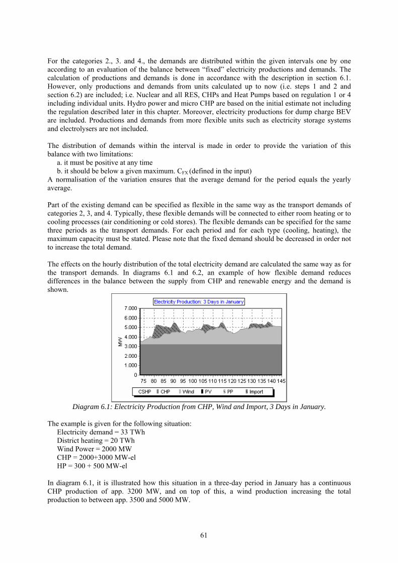
61

For the categories 2., 3. and 4., the demands are distributed within the given intervals one by one according to an evaluation of the balance between “fixed” electricity productions and demands. The calculation of productions and demands is done in accordance with the description in section 6.1. However, only productions and demands from units calculated up to now (i.e. steps 1 and 2 and section 6.2) are included; i.e. Nuclear and all RES, CHPs and Heat Pumps based on regulation 1 or 4 including individual units. Hydro power and micro CHP are based on the initial estimate not including the regulation described later in this chapter. Moreover, electricity productions for dump charge BEV are included. Productions and demands from more flexible units such as electricity storage systems and electrolysers are not included. The distribution of demands within the interval is made in order to provide the variation of this balance with two limitations:

a. it must be positive at any time b. it should be below a given maximum. CFX (defined in the input)

A normalisation of the variation ensures that the average demand for the period equals the yearly average. Part of the existing demand can be specified as flexible in the same way as the transport demands of categories 2, 3, and 4. Typically, these flexible demands will be connected to either room heating or to cooling processes (air conditioning or cold stores). The flexible demands can be specified for the same three periods as the transport demands. For each period and for each type (cooling, heating), the maximum capacity must be stated. Please note that the fixed demand should be decreased in order not to increase the total demand. The effects on the hourly distribution of the total electricity demand are calculated the same way as for the transport demands. In diagrams 6.1 and 6.2, an example of how flexible demand reduces differences in the balance between the supply from CHP and renewable energy and the demand is shown.

Diagram 6.1: Electricity Production from CHP, Wind and Import, 3 Days in January.

The example is given for the following situation:

Electricity demand = 33 TWh District heating = 20 TWh Wind Power = 2000 MW CHP = 2000+3000 MW-el HP = 300 + 500 MW-el

In diagram 6.1, it is illustrated how this situation in a three-day period in January has a continuous CHP production of app. 3200 MW, and on top of this, a wind production increasing the total production to between app. 3500 and 5000 MW.

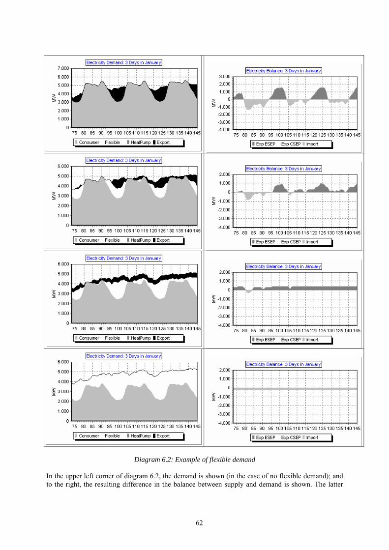
62

Diagram 6.2: Example of flexible demand

In the upper left corner of diagram 6.2, the demand is shown (in the case of no flexible demand); and to the right, the resulting difference in the balance between supply and demand is shown. The latter

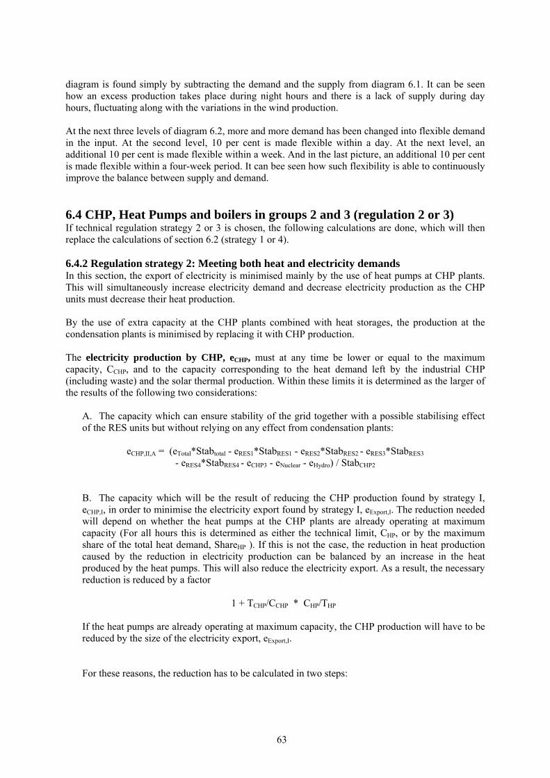
63

diagram is found simply by subtracting the demand and the supply from diagram 6.1. It can be seen how an excess production takes place during night hours and there is a lack of supply during day hours, fluctuating along with the variations in the wind production. At the next three levels of diagram 6.2, more and more demand has been changed into flexible demand in the input. At the second level, 10 per cent is made flexible within a day. At the next level, an additional 10 per cent is made flexible within a week. And in the last picture, an additional 10 per cent is made flexible within a four-week period. It can bee seen how such flexibility is able to continuously improve the balance between supply and demand. 6.4 CHP, Heat Pumps and boilers in groups 2 and 3 (regulation 2 or 3) If technical regulation strategy 2 or 3 is chosen, the following calculations are done, which will then replace the calculations of section 6.2 (strategy 1 or 4). 6.4.2 Regulation strategy 2: Meeting both heat and electricity demands In this section, the export of electricity is minimised mainly by the use of heat pumps at CHP plants. This will simultaneously increase electricity demand and decrease electricity production as the CHP units must decrease their heat production. By the use of extra capacity at the CHP plants combined with heat storages, the production at the condensation plants is minimised by replacing it with CHP production. The electricity production by CHP, eCHP, must at any time be lower or equal to the maximum capacity, CCHP, and to the capacity corresponding to the heat demand left by the industrial CHP (including waste) and the solar thermal production. Within these limits it is determined as the larger of the results of the following two considerations:

A. The capacity which can ensure stability of the grid together with a possible stabilising effect of the RES units but without relying on any effect from condensation plants:

eCHP,II,A = (eTotal*Stabtotal - eRES1*StabRES1 - eRES2*StabRES2 - eRES3*StabRES3

- eRES4*StabRES4 - eCHP3 - eNuclear - eHydro) / StabCHP2

B. The capacity which will be the result of reducing the CHP production found by strategy I, eCHP,I, in order to minimise the electricity export found by strategy I, eExport,I. The reduction needed will depend on whether the heat pumps at the CHP plants are already operating at maximum capacity (For all hours this is determined as either the technical limit, CHP, or by the maximum share of the total heat demand, ShareHP ). If this is not the case, the reduction in heat production caused by the reduction in electricity production can be balanced by an increase in the heat produced by the heat pumps. This will also reduce the electricity export. As a result, the necessary reduction is reduced by a factor

1 + TCHP/CCHP * CHP/THP

If the heat pumps are already operating at maximum capacity, the CHP production will have to be reduced by the size of the electricity export, eExport,I. For these reasons, the reduction has to be calculated in two steps:

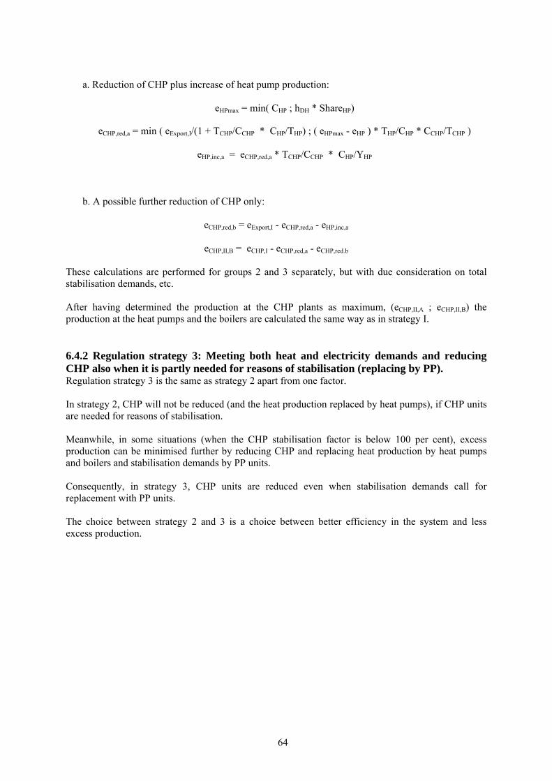
64

a. Reduction of CHP plus increase of heat pump production:

eHPmax = min( CHP ; hDH * ShareHP)

eCHP,red,a = min ( eExport,I/(1 + TCHP/CCHP * CHP/THP) ; ( eHPmax - eHP ) * THP/CHP * CCHP/TCHP )

eHP,inc,a = eCHP,red,a * TCHP/CCHP * CHP/YHP

b. A possible further reduction of CHP only:

eCHP,red,b = eExport,I - eCHP,red,a - eHP,inc,a

eCHP,II,B = eCHP,I - eCHP,red,a - eCHP,red.b

These calculations are performed for groups 2 and 3 separately, but with due consideration on total stabilisation demands, etc. After having determined the production at the CHP plants as maximum, (eCHP,II,A ; eCHP,II,B) the production at the heat pumps and the boilers are calculated the same way as in strategy I. 6.4.2 Regulation strategy 3: Meeting both heat and electricity demands and reducing CHP also when it is partly needed for reasons of stabilisation (replacing by PP). Regulation strategy 3 is the same as strategy 2 apart from one factor. In strategy 2, CHP will not be reduced (and the heat production replaced by heat pumps), if CHP units are needed for reasons of stabilisation. Meanwhile, in some situations (when the CHP stabilisation factor is below 100 per cent), excess production can be minimised further by reducing CHP and replacing heat production by heat pumps and boilers and stabilisation demands by PP units. Consequently, in strategy 3, CHP units are reduced even when stabilisation demands call for replacement with PP units. The choice between strategy 2 and 3 is a choice between better efficiency in the system and less excess production.

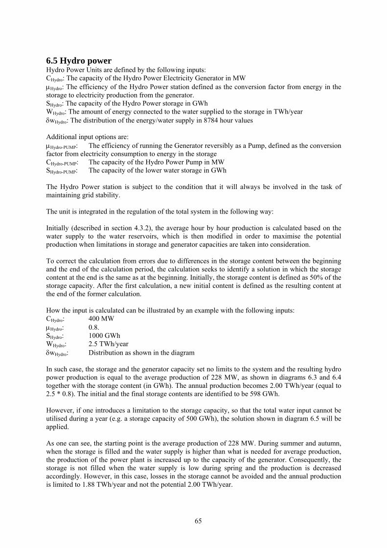
65

6.5 Hydro power Hydro Power Units are defined by the following inputs: CHydro: The capacity of the Hydro Power Electricity Generator in MW μHydro: The efficiency of the Hydro Power station defined as the conversion factor from energy in the storage to electricity production from the generator. SHydro: The capacity of the Hydro Power storage in GWh WHydro: The amount of energy connected to the water supplied to the storage in TWh/year δwHydro: The distribution of the energy/water supply in 8784 hour values Additional input options are: μHydro-PUMP: The efficiency of running the Generator reversibly as a Pump, defined as the conversion factor from electricity consumption to energy in the storage CHydro-PUMP: The capacity of the Hydro Power Pump in MW SHydro-PUMP: The capacity of the lower water storage in GWh The Hydro Power station is subject to the condition that it will always be involved in the task of maintaining grid stability. The unit is integrated in the regulation of the total system in the following way: Initially (described in section 4.3.2), the average hour by hour production is calculated based on the water supply to the water reservoirs, which is then modified in order to maximise the potential production when limitations in storage and generator capacities are taken into consideration. To correct the calculation from errors due to differences in the storage content between the beginning and the end of the calculation period, the calculation seeks to identify a solution in which the storage content at the end is the same as at the beginning. Initially, the storage content is defined as 50% of the storage capacity. After the first calculation, a new initial content is defined as the resulting content at the end of the former calculation. How the input is calculated can be illustrated by an example with the following inputs: CHydro: 400 MW μHydro: 0.8. SHydro: 1000 GWh WHydro: 2.5 TWh/year δwHydro: Distribution as shown in the diagram

In such case, the storage and the generator capacity set no limits to the system and the resulting hydro power production is equal to the average production of 228 MW, as shown in diagrams 6.3 and 6.4 together with the storage content (in GWh). The annual production becomes 2.00 TWh/year (equal to 2.5 * 0.8). The initial and the final storage contents are identified to be 598 GWh. However, if one introduces a limitation to the storage capacity, so that the total water input cannot be utilised during a year (e.g. a storage capacity of 500 GWh), the solution shown in diagram 6.5 will be applied. As one can see, the starting point is the average production of 228 MW. During summer and autumn, when the storage is filled and the water supply is higher than what is needed for average production, the production of the power plant is increased up to the capacity of the generator. Consequently, the storage is not filled when the water supply is low during spring and the production is decreased accordingly. However, in this case, losses in the storage cannot be avoided and the annual production is limited to 1.88 TWh/year and not the potential 2.00 TWh/year.

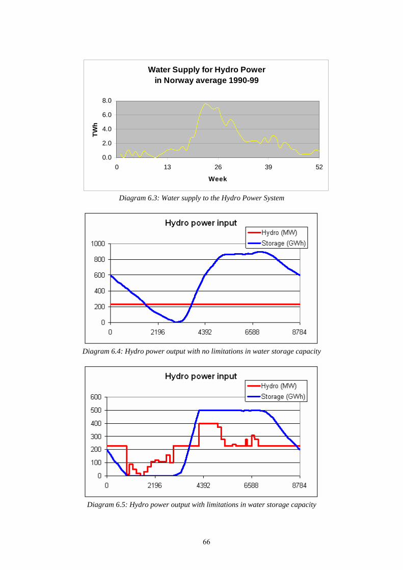
66

Water Supply for Hydro Power in Norway average 1990-99

0.0

2.0

4.0

6.0

8.0

0 13 26 39 52

Week

TWh

Diagram 6.3: Water supply to the Hydro Power System

Diagram 6.4: Hydro power output with no limitations in water storage capacity

Diagram 6.5: Hydro power output with limitations in water storage capacity

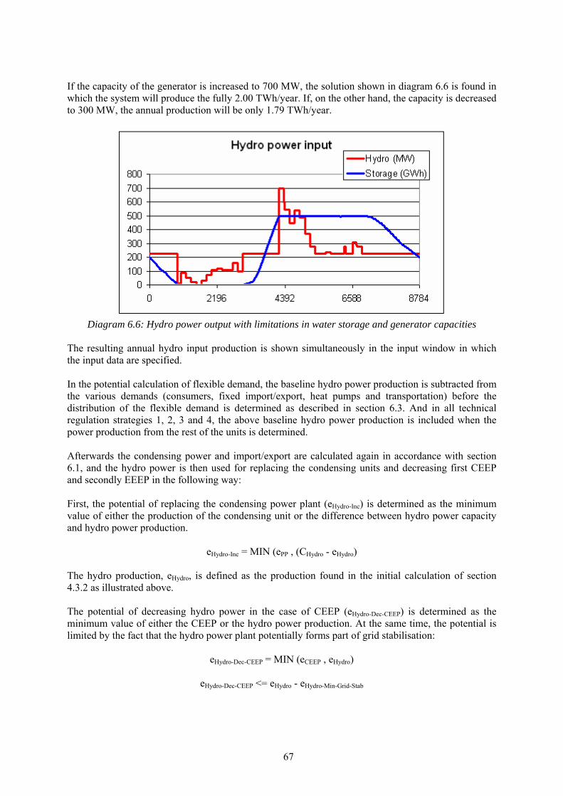
67

If the capacity of the generator is increased to 700 MW, the solution shown in diagram 6.6 is found in which the system will produce the fully 2.00 TWh/year. If, on the other hand, the capacity is decreased to 300 MW, the annual production will be only 1.79 TWh/year.

Diagram 6.6: Hydro power output with limitations in water storage and generator capacities

The resulting annual hydro input production is shown simultaneously in the input window in which the input data are specified. In the potential calculation of flexible demand, the baseline hydro power production is subtracted from the various demands (consumers, fixed import/export, heat pumps and transportation) before the distribution of the flexible demand is determined as described in section 6.3. And in all technical regulation strategies 1, 2, 3 and 4, the above baseline hydro power production is included when the power production from the rest of the units is determined. Afterwards the condensing power and import/export are calculated again in accordance with section 6.1, and the hydro power is then used for replacing the condensing units and decreasing first CEEP and secondly EEEP in the following way: First, the potential of replacing the condensing power plant (eHydro-Inc) is determined as the minimum value of either the production of the condensing unit or the difference between hydro power capacity and hydro power production.

eHydro-Inc = MIN (ePP , (CHydro - eHydro) The hydro production, eHydro, is defined as the production found in the initial calculation of section 4.3.2 as illustrated above. The potential of decreasing hydro power in the case of CEEP (eHydro-Dec-CEEP) is determined as the minimum value of either the CEEP or the hydro power production. At the same time, the potential is limited by the fact that the hydro power plant potentially forms part of grid stabilisation:

eHydro-Dec-CEEP = MIN (eCEEP , eHydro)

eHydro-Dec-CEEP <= eHydro - eHydro-Min-Grid-Stab

68

In the case of reversal hydro power, i.e. a pump and lower water storage, the potential of decreasing CEEP further (eHydro-Pump-Dec-CEEP) is determined as the minimum value of the CEEP (minus the share that is already occupied), the pump capacity, or the content of the lower water storage, sHydro-PUMP:

eHydro-Pump-Dec-CEEP = MIN [(eCEEP - eHydro-Dec-CEEP) , CHydro-PUMP , sHydro-PUMP / μHydro-PUMP ] In the same way, the potential of decreasing hydro power in the case of EEEP (eHydro-DEC-EEEP) is found. Knowing the potentials of increasing and decreasing the hydro power production, a balance is found in which the annual hydro power production is maintained. The reduction of CEEP is given priority over the reduction in EEEP.

Σ eHydro-Inc = Σ eHydro-Dec-CEEP + Σ eHydro-Dec-EEEP Similar to the previous modelling of the hydro power input, the programme again calculates the hour by hour modelling of the system including the fluctuations in the storage content. The hydro power production (eHydro) is modified in accordance with the generator capacity, the distribution of the water supply and the storage capacity in the following way:

Hydro-storage-content = Hydro-storage content + wHydro

eHydro = eHydro + eHydro-Inc - eHydro-Dec-CEEP - eHydro-Dec-EEEP

eHydro-Input <= (Hydro-storage-content - SHydro)* μHydro

eHydro-Input <= CHydro Differences in the storage content at the beginning and at the end of the calculation period may cause errors in the calculations. To correct these errors, the above calculation seeks to identify a solution in which the storage content at the end is the same as at the beginning. Initially, the storage content is defined as 50% of the storage capacity. After the first calculation, a new initial content is defined as the resulting content at the end of the former calculation. How the input is calculated can be illustrated by the example in diagram 6.7. The upper diagram shows the electricity production for a week in a system with a high share of both CHP and wind power. The system has a high excess electricity production (CEEP). The next diagram shows the influence of the hydro input (before the hydro regulation). It can be seen how the hydro power automatically replaces the power plant (PP) in the situations in which the PP produces in order to secure grid stability. However, in other situations, the hydro power also adds to the problem of excess production. In the third diagram, the hydro power is part of the regulation and it can bee seen how the hydro power plant is used for replacing the condensing plant and reducing the excess production.

69

Electricity production without hydro

0100020003000400050006000700080009000

1 14 27 40 53 66 79 92 105 118 131 144 157

CEEPWindPPHydroCHP

Annual (TWh/year): CEEP: 2.19 PP: 10.79 Hydro: 0.00

Electricity production BEFORE hydro regulation

0100020003000400050006000700080009000

1 14 27 40 53 66 79 92 105 118 131 144 157

CEEPWindPPHydroCHP

Annual (TWh/year): CEEP: 3.23 PP: 3.88 Hydro: 8.00

Electricity production AFTER Hydro Regulation

0100020003000400050006000700080009000

1 14 27 40 53 66 79 92 105 118 131 144 157

CEEPWindPPHydroCHP

Annual (TWh/year): CEEP: 2.19 PP: 2.80 Hydro: 8.00

Diagram 6.7:Hydro power is regulated to decrease excess and condensing power productions.

70

6.6 Individual CHP and Heat Pump systems The calculations of individual CHP and Heat Pumps systems are based on the initial calculations of section 4.6. If heat storage capacity is specified then the following moderation will be carried out and replace the previous productions. 6.6.1 CHP systems Heat production and the use of the heat storage give priority to solar thermal, which is calculated as the maximum value of either solar thermal production or heat demand plus available room in the heat storage:

qSolar-M-H2CHP = Max [qSolar-M-H2CHP , hM-H2CHP + (SSolar-M-H2CHP – sSolar-M-H2CHP) ] In case of CEEP If the solar production is lower than the heat demand and CEEP is positive then the heat demand will be supplied by the heat storage if possible. Only in the case that this can not be done, the CHP unit will be operated. Consequently, the CHP heat production is calculated as follows:

qM-H2CHP = Max [0 , (hM-H2CHP - sSolar-M-H2CHP - qSolar-M-H2CHP)] If such CHP heat production exceeds the capacity then the boiler is operated and the CHP heat production is reduced to the capacity

qM-H2CHP-Boiler = Max [0 , (TM-H2CHP - qM-H2CHP)]

qM-H2CHP = Min [qM-H2CHP , TM-H2CHP] In case of condensing power production If the condensing power production is positive then the micro CHP unit will try to produce at maximum capacity. And only in the case that excess heat production can not be stored, the CHP unit will be decreased accordingly. Consequently, the CHP heat production is calculated as follows:

qM-H2CHP = Min [TM-H2CHP , (hM-H2CHP - qSolar-M-H2CHP + (SSolar-M-H2CHP - sSolar-M-H2CHP))] The calculations are done separately for each of the three micro CHP systems starting with the H2-CHP system, followed by the Ngas system and the Biomass system. In between each calculation, the condensing power and excess productions are calculated. 6.6.2 Heat pump system After calculating the CHP systems, the heat pumps systems are calculated in the following way. Like the CHP system, the heat production and the use of the heat storage give priority to solar thermal, which is calculated as the maximum value of either solar thermal or heat demand plus available room in the heat storage:

qSolar-M-HP = Max [qSolar-M-HP , hM-HP + (SSolar-M-HP – sSolar-M-HP) ] In case of condensing power production If the solar production is lower than the heat demand and the production on the condensing power plant is positive, then the heat demand will be supplied by the heat storage if possible. And only in the case that this can not be done, the heat pump units will be operated. Consequently, the heat pump heat production is calculated as follows:

qM-HP = Max [0 , (hM-HP - sSolar-M-HP - qSolar-M-HP)]

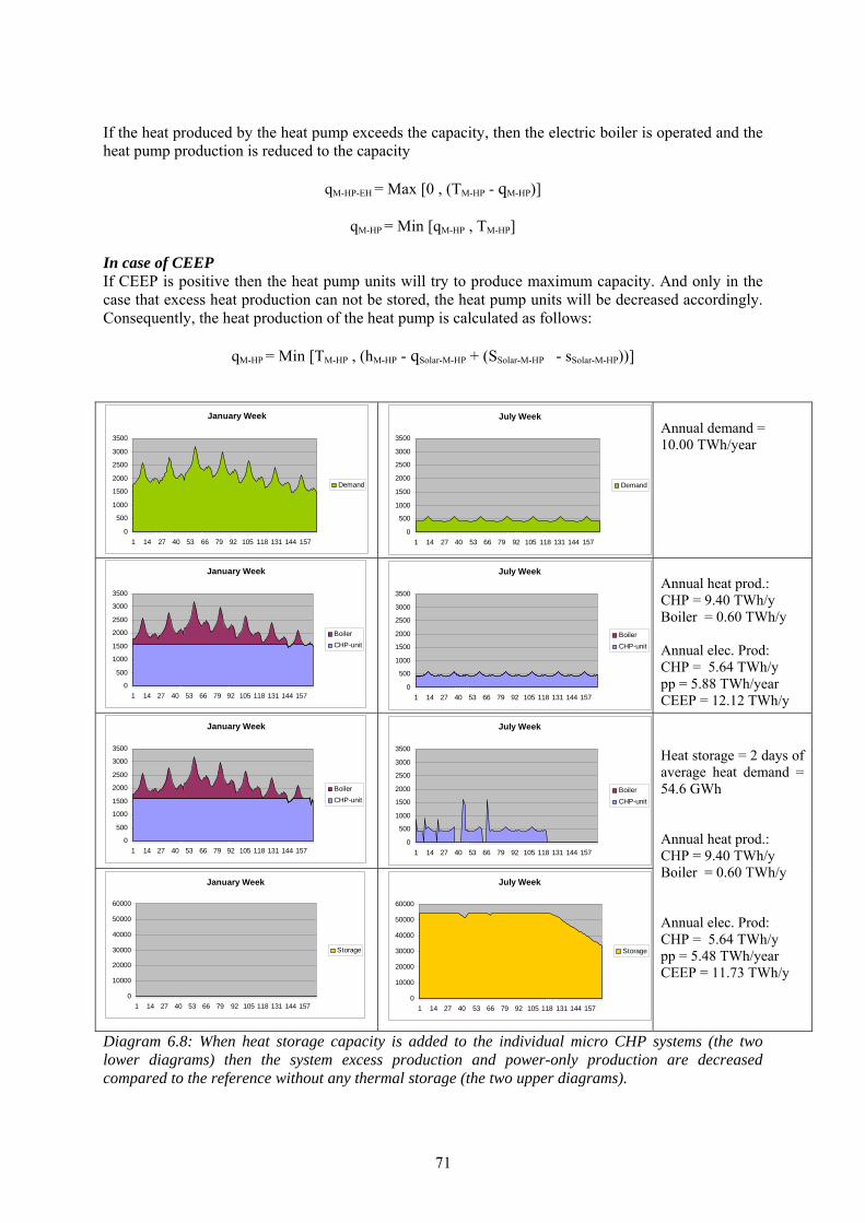
71

If the heat produced by the heat pump exceeds the capacity, then the electric boiler is operated and the heat pump production is reduced to the capacity

qM-HP-EH = Max [0 , (TM-HP - qM-HP)]

qM-HP = Min [qM-HP , TM-HP] In case of CEEP If CEEP is positive then the heat pump units will try to produce maximum capacity. And only in the case that excess heat production can not be stored, the heat pump units will be decreased accordingly. Consequently, the heat production of the heat pump is calculated as follows:

qM-HP = Min [TM-HP , (hM-HP - qSolar-M-HP + (SSolar-M-HP - sSolar-M-HP))]

January Week

0

500

1000

1500

2000

2500

3000

3500

1 14 27 40 53 66 79 92 105 118 131 144 157

Demand

July Week

0

500

1000

1500

2000

2500

3000

3500

1 14 27 40 53 66 79 92 105 118 131 144 157

Demand

Annual demand = 10.00 TWh/year

January Week

0

500

1000

1500

2000

2500

3000

3500

1 14 27 40 53 66 79 92 105 118 131 144 157

BoilerCHP-unit

July Week

0

500

1000

1500

2000

2500

3000

3500

1 14 27 40 53 66 79 92 105 118 131 144 157

BoilerCHP-unit

Annual heat prod.: CHP = 9.40 TWh/y Boiler = 0.60 TWh/y Annual elec. Prod: CHP = 5.64 TWh/y pp = 5.88 TWh/year CEEP = 12.12 TWh/y

January Week

0

500

1000

1500

2000

2500

3000

3500

1 14 27 40 53 66 79 92 105 118 131 144 157

BoilerCHP-unit

July Week

0

500

1000

1500

2000

2500

3000

3500

1 14 27 40 53 66 79 92 105 118 131 144 157

BoilerCHP-unit

January Week

0

10000

20000

30000

40000

50000

60000

1 14 27 40 53 66 79 92 105 118 131 144 157

Storage

July Week

0

10000

20000

30000

40000

50000

60000

1 14 27 40 53 66 79 92 105 118 131 144 157

Storage

Heat storage = 2 days of average heat demand = 54.6 GWh Annual heat prod.: CHP = 9.40 TWh/y Boiler = 0.60 TWh/y Annual elec. Prod: CHP = 5.64 TWh/y pp = 5.48 TWh/year CEEP = 11.73 TWh/y

Diagram 6.8: When heat storage capacity is added to the individual micro CHP systems (the two lower diagrams) then the system excess production and power-only production are decreased compared to the reference without any thermal storage (the two upper diagrams).

72

Diagram 6.8 illustrates how the model functions in the case of no solar thermal production. An annual heat demand of 10 TWh/year is specified and the resulting hour distribution is shown in the upper diagrams for a week in January and a week in July. The next diagram shows the production in the same weeks divided between the CHP unit and the peak load boiler. On an annual basis, the CHP unit produces 9.40 TWh and the boiler produces 0.60 TWh heat. The electricity production of the CHP units is 5.64 and, in the example, the power plant’s production is 5.88 TWh/year and the excess production is 12.12 TWh/year. The two lower diagrams show how the model changes the productions IF heat storage capacity is added. The annual heat and electricity productions from the CHP unit are the same, but the heat storage allows for a decrease in the power plant production and the excess production of the total system. In diagram 6.9, the same calculations are shown in which solar thermal is added to the system. I such case, the model gives priority to the utilisation of the solar thermal input. In the two upper diagrams without heat storage capacity, the solar thermal input can not be fully utilised. When storage capacity is added then such capacity is first used in order to increase the utilisation of solar thermal from 1.25 to 1.49 TWh/year, and then to decrease power-only production and the excess production of the system.

January Week

0

500

1000

1500

2000

2500

3000

3500

1 14 27 40 53 66 79 92 105 118 131 144 157

Demand

July Week

0

500

1000

1500

2000

2500

3000

3500

1 14 27 40 53 66 79 92 105 118 131 144 157

Demand

Annual demand = 10.00 TWh/year

January Week

0

500

1000

1500

2000

2500

3000

3500

1 14 27 40 53 66 79 92 105 118 131 144 157

BoilerCHP-unitSolar

July Week

0

500

1000

1500

2000

2500

3000

3500

1 14 27 40 53 66 79 92 105 118 131 144 157

BoilerCHP-unitSolar

Annual heat prod.: Solar = 1.25 TWh/y CHP = 8.23 TWh/y Boiler = 0.51 TWh/y Annual elec. Prod: CHP = 4.94 TWh/y pp = 6.24 TWh/year CEEP = 11.78 TWh/y

January Week

0

500

1000

1500

2000

2500

3000

3500

1 14 27 40 53 66 79 92 105 118 131 144 157

BoilerCHP-unitSolar

July Week

0

500

1000

1500

2000

2500

3000

3500

1 14 27 40 53 66 79 92 105 118 131 144 157

BoilerCHP-unitSolar

January Week

0

10000

20000

30000

40000

50000

60000

1 14 27 40 53 66 79 92 105 118 131 144 157

Storage

July Week

0

10000

20000

30000

40000

50000

60000

1 14 27 40 53 66 79 92 105 118 131 144 157

Storage

Heat storage = 2 days of average heat demand = 54.6 GWh Annual heat prod.: Solar = 1.49 TWh/y CHP = 8.00 TWh/y Boiler = 0.51 TWh/y Annual elec. Prod: CHP = 4.80 TWh/y pp = 5.96 TWh/year CEEP = 11.36 TWh/y

Diagram 6.9: Corresponds to diagram 6.8 plus solar thermal, which is then prioritized.

73

6.7 Electrolyser for micro CHP, Transportation, DH groups 2 and 3 Four electrolyser systems are described in the model. Two of these are systems which are meant to be located next to the district heating groups 2 and 3 along with the CHP units, Heat Pumps and boilers. Here, the heat production of the electrolysers can be utilised in the district heating supply. The two other systems produce hydrogen for micro CHP systems and for transportation. The electrolyser is meant to be a hydrolyser (producing hydrogen) but can be used for modelling any kind of equipment converting electricity into fuel and heat. 6.7.1 Electrolysers for hydrogen production to individual micro CHP systems The calculation is based on the result of the input calculation in section 4.6.4., in which the minimum capacity of the electrolyser is identified together with the electricity demand dElcM. The model seeks to reorganise such production in order to avoid excess and power-only productions. First, the potential of increasing the production at hours of excess production is identified as the lower value of either CEEP or the difference between the capacity and the production of the electrolyser:

dElcM-inc-pot = Min [ eCEEP , (CElcM – dElcM) ] Secondly, the potential of decreasing production at hours of power-only production is identified as the lower value of either the power production or the electrolyser demand.

dElcM-dec-pot = Min [ ePP , dElcM ] Then a balance is created in which either the potential of increasing or the potential of decreasing is lowered so that the annual potentials are the same:

If DElcM-dec-pot > DElcM-inc-pot then dElcM-dec-pot = dElcM-dec-pot * DElcM-inc-pot / DElcM-dec-pot

If DElcM-inc-pot > DElcM-dec-pot then dElcM-inc-pot = dElcM-inc-pot * DElcM-dec-pot / DElcM-inc-pot A new optimal distribution of the electrolyser electricity demand (producing exactly the same annual fuel as before) is calculated as:

dElcM = dElcM - dElcM-dec-pot + dElcM-inc-pot Finally, such distribution is evaluated against the hydrogen storage capacity. First, the changes in storage content sElcM are calculated

sElcM(x) = sElcM(x-1) + dElcM(x) * αElcM - fM-NgasCHP-Total (x) If the storage content based on such calculation is below zero, the production on the electrolyser is raised:

If sElcM < 0 then dElcM = dElcM + (– sElcM / αElcM)

And if the storage content exceeds the storage capacity then the production on the electrolyser is decreased:

If sElcM > SElcM then dElcM = dElcM + (sElcM - SElcM) 6.7.2 Electrolysers for hydrogen production to transportation After calculating the regulation of the electrolyser for individual micro hydrogen CHP systems the calculation of excess and power-only production (section 6.1) is repeated, and then the calculation of

74

the hydrogen production for transportation is done exactly the same way as for the micro CHP, as described above in section 6.7.1. 6.7.3 Electrolysers in district heating systems The regulation of the electrolysers in the district heating system is used solely in order to avoid critical excess electricity production, exactly as the two other electrolysers. However, the electrolysers in the district heating system do not have to produce a certain amount of hydrogen (as the two other electrolysers, which have to fulfil the demands of the hydrogen CHP and transportation systems). The sequence of the calculations is as follows. First, the electrolysers of district heating groups 3 and 2 are calculated. After each calculation, the calculation of excess production (section 6.1) is repeated. The electrolysers in each of the district heating systems are regulated in the following way: The electrolyser is used for producing fuel in the case of critical excess production, eCEEP>0. The fuel is used for reducing the fuel consumption of the CHP unit and the boiler of the particular group. If the thermal efficiency is equal to 0, then the use of electrolysers is simply calculated as the minimum value of either the CEEP value or the capacity of the electrolysers.

If ρElc = 0 Then eElc = min (eCEEP, CElc) If the thermal efficiency is positive, the heat of the electrolyser is used for reducing heat production of other units according to the following priority:

- reduce boiler production - reduce CHP production - reduce heat pump production - wasted

Step1: Replace boiler heat production First, the potential replacement of the boiler is calculated as the minimum value of either (1) the critical excess production, (2) the capacity of the electrolyser, or (3) the electricity consumption responding to the heat production of the boiler. The latter is found as the heat production of the boiler divided by the thermal efficiency of the electrolyser. The excess production and the productions of the boiler and the electrolyser are then adjusted accordingly.

Potential = min (eCEEP , CElc , qB / ρElc)

eCEEP = eCEEP – Potential

eElC = Potential

qElc = Potential * ρElc

qB = qB - Potential* ρElc

Step 2: Replace CHP heat production If the excess production is still positive, then the potential decrease in the CHP unit is found, first by calculating the factor which will make it possible to remove critical excess production without creating import. This factor takes into account the fact that the replacement of the CHP by the electrolyser

75

influences the excess production, as the CHP production is decreased and the electrolyser consumption is increased. The factor is determined by the following equations:

δeCEEP = δeCHP + δeElc

δqCHP = δqElc

δqElc = δeElc * ρElc

δqCHP = δeCHP * ρCHP / μCHP The factor then becomes:

Factor = 1 + ρCHP / (μCHP * ρΕlc) The factor is used for identifying the potential replacement of the CHP in which the combination of the CHP decrease and the electrolyser increase outbalances the excess production. Consequently, the potential CHP reduction is found as the critical excess production divided by the factor. Again, the potential replacement of the CHP unit is found as the minimum value of either such reduction or the capacity of the electrolyser or the electricity consumption responding to the heat production of the CHP unit.

Potential = min [ eCEEP / Faktor , (CElc - eElc) , qCHP / ρElc ] In the case of group 3, the potential reduction in the heat production of the CHP unit is found as the difference between the actual production and the minimum production according to the regulation inputs.

In group 3: Potential = min [ eCEEP / Faktor , (CElc3 - eElc3) , (qCHP3 - qCHP3-minimum ) / ρElc ] Again, the excess production and the production of the CHP and the electrolyser are then adjusted accordingly similar to the previous case of the boiler. Step 3: Replace the heat production of the heat pump If the excess production is still positive then the potential decrease in the heat pump (HP) unit is found, first by calculating the factor which will make it possible to remove critical excess without creating import. This factor takes into account the fact that the replacement of the HP by the electrolyser influences the excess production, as HP production decreases and electrolyser consumption increases. The factor is determined by the following equations:

δeCEEP = δeHP + δeElc

δqHP = δqElc

δqElc = δeElc * ρElc

δqHP = δeHP * φHP And the factor then becomes:

Factor = φHP / ρElc - 1

76

The factor is used for identifying the potential replacement of the HP by which the combination of the HP decrease and the electrolyser increase outbalances the excess production. Consequently, the potential HP reduction is found as the critical excess production divided by the factor. Again, the potential replacement of the HP unit is found as the minimum value of either such reduction or the capacity of the electrolyser or the electricity consumption responding to the heat production on the HP unit.

Potential = min (eCEEP / Faktor , (CElc - eElc), qHP / ρElc) Again, the excess production and the production of the HP and the electrolyser are then adjusted accordingly similar to the previous case of the boiler and the CHP. Step 4: Electrolyser heat production is wasted If the excess production is still positive then the potential increase in the electrolyser is simply found as the minimum value of either the excess production or the remaining increase up to the capacity of the electrolyser.

Potential = min [ eCEEP , (CElc - eElc) ] The excess production and the production of the electrolyser are then adjusted accordingly. 6.8 Heat storage in groups 3 and 2 To improve the possibilities of minimising the electricity export, the heat storage capacity is included in the model for each of the district heating groups 2 and 3. Again, such storage capacities are used for minimising the excess and power-only productions in the system. In two situations, the storage can be loaded:

A: Increasing the use of HP in situations with electricity export. B: Moving the electricity production from condensing plants, epp to CHP plants

In two situations, the storage can be unloaded:

C: Reducing the CHP production in situations with electricity export D: Reducing the boiler production.

B is secondary to A, and D is secondary to C. The four loading and unloading cases are used in the following order: C-A-B-D. These series are then used in the following order:

1: Critical excess electricity production eCEEP and CHP in group 3 2: Critical excess electricity production eCEEP and CHP in group 2 3: Exportable excess electricity export, eEEEP and CHP in group 3 4: Exportable excess electricity export, eEEEP and CHP in group 2

In order to achieve balance, the calculations are performed over a series of 2-week periods, in which the storage content at the end of the year is equal to the storage content at the beginning of the year. The four loading and unloading situations are calculated as follows: A: loading by increasing the use of HP in situations with electricity export. First, the minor of the potential increase in district heating production from HP, qHP-inc and the potential increase in storage content, sinc are determined.

77

qHP-inc = min (eEEP , CHP-eHP) * (THP/CHP)

sinc = SDH – sDH New values can now be calculated:

eHP = eHP + min(qHP-inc , sinc) * (CHP/THP)

eEEP = eEEP - min(qHP-inc , sinc) * (CHP/THP)

qHP = qHP + min(qHP-inc , sinc)

sDH = sDH + min(qHP-inc , sinc)

B: Moving the electricity production from condensing plants, ePP, to CHP plants First, the minimum condensing power plant production needed in order to stabilise the grid is found (see section 6.1 for more details):

ePP-min = (eTotal*Stabtotal - eCHP2*StabCHP2 - eRES1*StabRES1 - eRES2*StabRES2 - eRES3*StabRES3 - eRES4*StabRES4 - eCHP3 - eNuclear - eHydro - eV2G) / (1 - Stabtotal)

Then the potential increase in district heating production from CHP, qCHP-inc, and the potential increase in storage content, sinc, are determined

qCHP-inc = min [ (CCHP – eCHP) ; (ePP – ePP-min) ]

sinc = SDH – sDH New values can now be calculated:

eCHP = eCHP + min(qCHP-inc , sinc) * (CCHP/TCHP)

ePP = ePP - min(qCHP-inc , sinc) * (CCHP/TCHP)

qCHP = cCHP + min(qCHP-inc , sinc)

sDH = sDH + min(qCHP-inc , sinc) C: Reducing the CHP production in situations with electricity export First, the minimum CHP production needed in order to stabilise the grid is found. In the case of district heating (DH) group 2:

eCHP2-min = (eTotal*Stabtotal - eRES1*StabRES1 - eRES2*StabRES2 - eRES3*StabRES3 - eRES4*StabRES4 – (ePP/ StabTotal) - eCHP3 - eNuclear - eHydro) / StabCHP2

And in the case of DH group 3:

eCHP3-min = eTotal*Stabtotal - eRES1*StabRES1 - eRES2*StabRES2 - eRES3*StabRES3 - eRES4*StabRES4 – (ePP/ StabTotal) - eNuclear - eHydro – (eCHP2/ StabCHP2 )

If eCHP3-min < CCHP3-min then eCHP3-min < CCHP3-min

78

Secondly, the potential of decreasing the CHP heat production, qCHP-red, is found as the lower value of either the excess production or the difference between the actual production and the minimum production required for grid stabilisation.

qCHP-red = min(eEEP ; eCHP – eCHP-min) * (TCHP/CCHP) New values can now be calculated:

eCHP = eCHP - min(qCHP-red , sDH) * (CCHP/TCHP)

eEEP = eEEP - min(qCHP-red , sDH) * (CCHP/TCHP)

qCHP = qCHP - min(qCHP-red , sDH)

sDH = sDH - min(qCHP-red , sDH) D: Reducing boiler production. First, the smallest potential reduction in boiler production, qB-red, and the potential reduction in storage content, sred, are determined:

qB-red = qB

New values can now be calculated:

qB = qB – min(qB-red ; sDH)

sDH = sDH - min(qB-red ; sDH)

79

6.9 Transportation (Smart charge and V2G) Definition of inputs: DV2G: Transportation Demand of V2G cars in TWh/year (defined as demand from the grid) δV2G: The distribution of the transportation demand in 8784 hourly values.

(The numbers are relative e.g. each ranging 0 to 1). CCharger: The capacity of the grid connection in MW V2GMaxShare: The maximum share of V2G cars which are driving during peak demand hour. μCharger: The efficiency of the grid to battery connection (charger). μInverter: The efficiency of the battery to grid connection (inverter). SV2G-Battry: The capacity of the battery storage in GWh V2GConnection-Share: The share of parked V2G cars connected to the grid. All inputs are expressed for the entire utility system analysed, and for the entire vehicle fleet within the service territory of that utility system. Thus, for example, the maximum system capacity CCharger is calculated on the basis of the line maximum power of a single car multiplied by the maximum number of vehicles plugged in at any given time. One important input is the distribution of the transportation demand (δV2G), which is used for two purposes. One is to determine how many V2G cars are driving and consequently not connected to the grid at the hour in question. This, together with the V2GMax-Share (the maximum share of V2G cars which are driving during peak demand hour) and the V2GConnection-Share, determines the fraction of the V2G fleet that is available to the electrical system at any given hour. The other purpose for δV2G is to determine the discharging of the battery storage for driving. Initial input calculations The hourly transportation demand and thereby the discharging of the battery (tV2G) is calculated as follows:

tV2G = [ DV2G * δV2G / Σ δV2G ] * ηCHARGE The grid connection capacity of the total V2G fleet on an hourly basis (cV2G) will be calculated as follows:

cV2G = CCharger * V2GConnection-Share * ((1- V2GMax-Share) + V2GMax-Share *(1 - δV2G/Max(δV2G))

This formula is constituted by three factors. The first factor is CCharger , the power capacity of the entire V2G fleet. This is multiplied by V2GConnection-Share, the fraction of the parked vehicles which is assumed to be plugged. The third factor, in parentheses, calculates the fraction of vehicles on the road at each hour. Further decomposing the third parenthesized factor, it consists of the sum of two terms. The first term, (1- V2GMax-Share), represents the minimum fraction of vehicles parked. The second term is the additional fraction of vehicles parked during non-rush hours. The hourly fraction of vehicles parked is derived from the known input of hourly energy demand for the fleet. This formula yields cV2G , the power capacity of all connected V2G vehicles, at any given hour. This is a calculation of capacity, not considering whether sufficient battery power is available; the latter is treated in the next section. The calculation works as described in the following example of 1.9 million cars, each with a grid connection of 10 kW and each with a demand of 2 MWh/year equal to 20,000 km/year. The charger and inverter efficiencies are each defined as 0.9. In total, the demand for transportation becomes DV2G=3.8 TWh/year and a maximum capacity of 19,000 MW. The power used is distributed between a peak demand during rush hours between 7:00 and 9:00 a.m. and another one between 16:00 and 18:00 p.m., as shown in the diagram for one week (Please, recall that this is battery demand, not electric system demand, as the vehicles are necessarily disconnected from the grid while driving).

80

Distribution input

0

0.2

0.4

0.6

0.8

1

0 24 48 72 96 120 144 168

hour

Diagram 6.10: Input distribution of transportation demand

Based on such information, the model will calculate the distribution of the demand and thereby also the discharging of the battery, as shown in the next diagram. The sum of the diagram within a year becomes 3.42 TWh/year equal to 0.9 * 3.8 TWh/year.

Demand / discharging of battery in MWh/h

0

250

500

750

1000

0 24 48 72 96 120 144 168

hour

Diagram 6.11: Transportation demand and discharging of battery.

The calculation of the available grid connection depends on the definition of both the maximum share of V2G cars, V2GMaxShare, and the share of parked vehicles which are connected, V2GConnectionShare. If both are 100 per cent, the result is as shown in the upper figure of diagram 6.12. In such case, the model assumes that all vehicles are driving during peak demand and, consequently, the grid connection becomes zero. During low demand, the grid connection becomes equal to the maximum grid connection CCharger, subtracting the few vehicles that are driving. Even during peak demand (rush hour), the model does not assume all vehicles to be driving. By setting the V2GMaxShare value one can define how many cars are parked and potentially connected to the grid during peak demand. In diagram 6.12, (the figure in the middle), the V2GMaxShare has been defined as 20 per cent representing a typical situation in which a minimum of 80 per cent of all cars are parked during rush hours (Kempton et al 2001).

81

Grid connection in MWV2G-max-share = 1, V2Gconnection-share = 1

0

5000

10000

15000

20000

0 24 48 72 96 120 144 168

hour

Grid connection in MWV2G-max-share = 0.2, V2Gconnection-share = 1

0

5000

10000

15000

20000

0 24 48 72 96 120 144 168

hour

Grid connection in MWV2G-max-share = 0.2, V2Gconnection-share = 0.7

0

5000

10000

15000

20000

0 24 48 72 96 120 144 168

hour

Diagram 6.12: The model calculation of the available grid connection for three different combinations

of input definitions.

82

In the lower figure of diagram 6.12, the input of the share of parked vehicles which are connected, V2GConnectionShare, has been changed from 100 to 70 per cent and, consequently, the grid connection is decreased in general by 30 per cent compared to fig 2. Considerations on the modelling of the battery and loading before disconnecting The batteries of the V2G fleet are modelled as if one “big battery” existed for the entire vehicle fleet. The available battery capacity is equal to the maximum capacity. In reality, the total capacity of the battery is not available all the time, since some of the cars will be driving, and can neither discharge to, nor charge from, the grid; others will need to drive during the next few hours and thus cannot be discharged. However, the model assumes for simplicity that the batteries for the cars are scheduled to be fully loaded when they disconnect and start driving. Consequently, the model does not gain much from keeping separate account on the share of the battery, which is not connected, since this part would typically within the hour be fully loaded anyway. However, the share representing the cars driving will discharge a bit from one hour to another in the case of cars driving for more than one hour. If one wants to take such issues into consideration, one could simply make a small reduction in the input value for the capacity of the battery, SV2G-Battery. The model is required to make sure that the individual car is fully loaded before it is planned to disconnect. In general, the batteries are loaded in the case of excess electric power production. However, when there is not excess power production, the model has to make sure that the batteries are loaded prior to driving periods. (In a future refinement of the model, we may assume that the vehicle controller is able to infer how much charge is needed and would not need to always fully charge if there is no excess production and vehicle use is highly regular; e.g. if intercity trips are only taken on Saturdays, the battery may not need to be fully charged at early mornings during weekdays.) The model assumes that the scheduler on each car is 100% accurate about when the driver will need to drive again. Therefore, the scheduler is assumed to prioritize charging of the cars that will drive again within the next few hours, so if there is only a small amount of excess wind, it is directed to the cars that will be in use next time. That is, during each hour, the model inspects the next e.g. two hours’ driving needs, and if there is not enough in the big battery for this, then the charging is forced even in the case of lack of excess production, specifically, if needed, fossil fuel power plants will be switched on if there is not enough excess wind. Such procedure simulates a situation in which the individual car owner will make priorities on how to optimise between low costs of charging and security of fully loaded batteries when starting to drive. The car owner does this by setting prices and limitations to the computer control of the car. However, the car owner will learn from experience, and will soon know how to optimise. He will also know how many hours in advance he must start the charging of the battery even in the case of no low prices. Here, the model on its own identifies the necessary number of hours to be able to secure driving and thereby the minimum battery loading. The necessary number of hours will depend on both the shape and pattern of the distribution of the transportation demand, as well as on the definition of the rest of the energy system. For example, a system in which the excess production is severe will call for less “pre-loading” than a system in which the excess production is small. The necessary hours of “pre-loading” is found by use of try-and-error. The model starts by assuring that the battery always has the minimum load required in order to supply the next one hour and if this results in lack of battery content the number is raised to two, etc. The number of hours becomes a result of the calculation. In an optimized electric control system, the number of hours prior to driving might also be determined by weather forecasts regarding anticipated wind for the next few hours, but we do not consider such refinements here.

83

Modelling of the V2G cars For each hour, the model calculates as follows. The V2G cars are told to charge in the case of available excess electricity production for that hour (eCEEP) and available battery energy capacity (SV2G-

Battery - sV2G-Battery) within the limitations of the power capacity of the grid connection (cV2G) for that hour. Thus, the formula takes the minimum of these three values:

eCharge = min [eCEEP, (SV2G-Battry - sV2G-Battery ) / μCharge , cV2G] Moreover, as mentioned above, the charging is forced in the case in which the transport demands of the present and the next “y” hours cannot be supplied by the battery content. Initially, the “y” value is set to one hour. If this leads to lack of battery content the value is raised in steps of one hour. The minimum battery content needed is calculated:

x=a sV2G-Battary-min = Σ tV2G a+y

Then the charging of the battery is adjusted accordingly, by requiring that:

eCharge >= [sV2G-battery - sV2G-Battary-min ] / μCharge If eCharge becomes higher than the capacity of the grid connection cV2G then the number of hours, y, is raised by one, and the calculations start all over again. The new battery content is then calculated by adding the above charging and subtracting the discharging caused by driving (tV2G):

sV2G-Battery := sV2G-Battery - tV2G + (eCharge / μCharge ) The V2G cars are told to supply to the grid in the case of potential replacement of production from power plants (ePP) and available stored electricity in the battery after the supply of the transportation demand:

eInv = min [ePP, ((sV2G-Battery - sV2G-Battery -min)* μInv ), cV2G ] The resulting new battery content is then calculated as follows

sV2G-Battery := sV2G-Battery - (eInv / μInv ) Due to differences in the battery storage content between the beginning and the end of the calculation period (one year), errors may appear in the calculations. To correct these errors, the above calculation is repeated until the storage content at the end is the same as at the beginning. Initially, the storage content is defined as 50% of the battery storage capacity. After the first calculation, a new initial content is defined as the resulting content at the end of the former calculation. Such procedure is repeated until the difference is insignificant. REFERENCES CITED: Kempton, W., J. Tomic, S. Letendre, A. Brooks & T. Lipman. 2001. Vehicle-to-Grid Power: Battery, Hybrid, and Fuel Cell Vehicles as Resources for Distributed Electric Power in California. UCD-ITS-RR-01-03. Kempton, Willett and Jasna Tomic, 2005a. Vehicle to Grid Fundamentals: Calculating Capacity and Net Revenue. J. Power Sources Volume 144, Issue 1, 1 June 2005, Pages 268-279. doi:10.1016/j.jpowsour.2004.12.025.

84

6.10 Electricity storage The electricity storage is described in the model as a hydro storage consisting of the following components:

- Pump (converting electricity to potential energy) defined by a capacity and an efficiency - Turbine (converting potential energy to electricity) defined by a capacity and an efficiency - Storage (storing energy) defined by a capacity.

Meanwhile, the hydro storage can be used for modelling any kind of electricity storage such as for example batteries. The regulation of the storage is used solely in order to avoid critical excess electricity production. The storage facility is regulated in the following way: The pump is used for filling the storage in the case of critical excess production, eCEEP > 0. In such case, the available space in the storage (SCAES – sCAES) is calculated and the electricity demand of the pump (ePump) is found as the minimum value of the following three figures:

- eCEEP, the critical excess production - (SCAES – sCAES) / αPump available storage capacity divided by the pump efficiency - CPump, the maximum capacity of the pump.

If eCEEP > 0 then ePump:= min [ eCEEP, (SCAES – sCAES) / αPump , CPump ]

sCAES = sCAES + ePump / αPump

The turbine is used for emptying the storage first by replacing import and then power plant production if ePP > 0. In such case, the content of the storage (sCAES) is identified and the electricity production of the turbine (eTurbine) is found as the minimum value of the following three figures:

- eimport, ePP, import or the electricity production of the power plant respectively - sCAES * μTurbine, storage content multiplied by the turbine efficiency - CTurbine, the maximum capacity of the turbine.

If eimport> 0 then eTurbine1:= min [eimport, sCAES * μTurbine, CTurbine]

If ePP> 0 then eTurbine2:= min [ePP, sCAES * μTurbine, (CTurbine- eTurbine1]

eTurbine = eTurbine1+ eTurbine2

sCAES = sCAES - eTurbine / μTurbine

Due to differences in the storage content between the beginning and the end of the calculation period, errors may appear in the calculations. In order to correct these errors, the above calculation is repeated until the storage content at the end is the same as at the beginning. Initially, the storage content is defined as 50% of the storage capacity. After the first calculation, a new initial content is defined as the resulting content at the end of the former calculation. Such procedure is repeated until the difference is insignificant. CAES (Compressed Air Energy Storage) The electricity storage facility can also be used to model a Compressed Air Energy Storage component. The CAES component is modelled in a similar way to the pumped hydro storage, the main difference being the fuel consumption at the electricity production stage. Consequently, one has to specify a CAES fuel ratio, φCAES, which is defined as fuel input divided by the electricity production of the turbine, eTurbine

85

Please, note that in CAES, the main loss in the storage is heat loss, which occurs only during the initial hours after compression. As a certain time usually elapses before the expansion phase begins, the heat loss in the storage is included in the compressor efficiency definition. The compressor is utilized in the model after calculating the heat and electricity production of the CHP and power plants, but before reducing excess electricity by use of other means. In the case of having pumped hydro storage into the system, this is prioritized over the CAES plant operation. The turbine is utilized in order to replace power plant production.

86

7. Market-Economic Optimisation If market-economic regulation is chosen in the input regulation window the following optimisation procedure is used. The model distinguishes between business economy (including taxes) and socio economy (NOT including taxes). Basically, the model identifies the lowest cost solution of the system, assuming an electricity market on which all plant operators seek to optimise their business-economic profit. 7.1 Net import and resulting external market price The market-economic modelling is based on the identification of the market price at each hour resulting from the demand and supply of electricity. Moreover, the exact production of the various units in which the resulting market price becomes equal to the marginal production price is identified. Similar balance prices are found for electricity-consuming units such as heat pumps and electrolysers. Consequently, the following types of calculations are done continuously as an integrated part of each of the following sequences (sections 7.2 – 7.9) in the market-economic optimisation procedure. 7.1.1 Calculating the resulting market price First, the net import is identified as the difference between the electricity demand dTotal and the supply eTotal:

dNet-Import = dTotal - eTotal

dTotal = dE + dEX + dFX + dCool + dBiogas + dElc + dBEV + dV2G + dI-HP-total + dI-EH + dHP2 + dHP3 + dPump + dHydroPump

in which dFX = dFXDay + dFXWeek + dFX4Week

and dElc = dElc2 + dElc3 + dElcT + dElcM

eTotal = ePP +eRES + eM-CHP + eHydro + eNuclear + eV2G + eW + eCSHP + eCHP2 + eCHP3 + eCHP3-MIN +eTurbine

in which eRES = eRES1 + eRES2 + eRES3 + eRES4

and eM-CHP = eM-h2CHP + eM-NgasCHP + eM-BioCHP

In the calculation of the net import, the production from CHP3 is divided into eCHP3 and eCHP3-Min as explained in section 7.3 below. The market price on the external market, pX, is now found as follows:

pX = pi + ( pi / po )* Facdepend * dNet-Import where pi is the system market price (see section 4.3),

Facdepend is the price elasticity (DKK/MWh/MW) po is the basic price level for price elasticity (input), dNet-Import is the trade on the market.

Import is calculated as positive and export is negative, resulting in an increase in the market price in case of import and a decrease in case of export.

87

7.1.2 Calculating the balance production The balance production from a certain unit in which the resulting market price becomes equal to the marginal production price is identified as an integrated part of the procedure. Here, such calculation is illustrated by the example of the geothermal power plant. First, the net-import, dNet-Import, is calculated as well as the market price, pX, as described above in section 7.1.1, when the electricity production of the geothermal power plant is zero. Then the balance production is calculated as follows:

BalanceProductionGeothermal = - [ ( VEPPGeothermal - pX ) / (Facdepend * pX / po ) - dNet-Import] where VEEPGeothermal is the marginal production cost of geothermal power production px is the market price before geothermal production (see section 7.1.1),

Facdepend is the price elasticity (DKK/MWh/MW) po is the basic price level for price elasticity (input), dNet-Import is the trade on the market before geothermal production

The formula is typically subject to the limitations of power plant capacity. 7.2 The overall procedure The optimisation is done in the following steps:

Step 1: Electricity Market Definition The electricity market is defined by the inputs in the Regulation window as described in section 4.13. The fluctuations of the market prices are presented as an hour by hour distribution file. One can change such prices by adding or multiplying figures as described in section 4.13. The influence of import/export on the external market prices is given in terms of a dependency factor (price elasticity and an basic price level for the price elasticity).

When the business-economic best operation strategy is identified for each plant in the following, the influence on the market price is taken into consideration.

Step 2: Identifying marginal production (and consumption) costs All marginal production costs are calculated on the basis of fuel costs, taxes, CO2 costs and variable operation costs as described in section 4.11. For units connected to district heating plants (such as CHP and heat pumps), power stations and individual micro CHP, marginal costs are given in DKK/MWh electricity production/consumption. For storage units such as hydrogen CHP and pump storage systems, marginal costs are given in a multiplication factor together with an addition factor. Basically, the optimisation criterion is the following:

psell > pbuy * fMUL + fADD

In which psell is the market electricity price when selling (DKK/MWh) pbuy is the market electricity price when buying (DKK/MWh) fMUL is the multiplication factor (always higher than 1), and fADD is the addition factor (DKK/MWh)

88

Step 3: Starting point electricity market prices As a starting point for the optimisation, the electricity system prices are calculated on the basis of:

- the electricity demand including flexible demand (calculated as described in section 6.3) - the production from RES (Wind power, PV etc.)

As a starting point, all district heating is defined as supplied from boilers.

Then the sequence of optimising the individual plants is identified by the subsequent procedure. Step 4: Optimising the buying of given hydrogen and electricity demands The lowest costs solutions of buying the minimum amount of electricity needed to meet the following demands are identified, given the market price fluctuations and limitations in storage capacities etc.:

- for producing hydrogen to transportation - for charging electric vehicles - for producing hydrogen for micro CHP systems

When identifying the lowest cost solution for the hydrogen micro CHP systems, the option of producing heat on a boiler using less hydrogen than the CHP unit is considered in situations of high electricity prices. In the case of V2G (Vehicle to Grid) possibilities, the optimal business-economic solutions of buying and selling are found on the basis of the multiplication and addition factors identified in the Cost Operation window (see section 4.11). Step 5: Optimising electricity consumption options Then the following electricity-consuming options are sorted according to the highest marginal consumption costs:

- replacing boiler with heat pumps in district heating group 2 - replacing boiler with heat pumps in district heating group 3 - replacing boiler with electrolysers in district heating group 2 - replacing boiler with electrolysers in district heating group 3 - replacing electric heating with heat pumps in individual houses

Each option is then optimised according to market electricity prices, starting with the option with the highest marginal costs and taking into consideration the fact that each change in consumption influences the market price (increases the price).

Step 6: Optimising hydro power Then the best business-economic production from hydro power is identified taking into consideration limitations in storage and generator capacities.

In the case of pump possibilities, the optimal business-economic solution of buying and selling are identified on the basis of the multiplication and addition factors identified in the Cost Operation window (see section 4.11). Step 7: Optimising electricity production options Then the following electricity production options are sorted according to the lowest marginal costs of production:

- Nuclear - Geothermal - Condensing Power plants - Individual Ngas CHP - Individual Biomass CHP - CHP replacing boilers in gr.2 - CHP replacing boilers in gr.3

89

- CHP replacing heat pumps in gr. 2 - CHP replacing heat pumps in gr. 3 - CHP replacing electrolysers in gr. 2 - CHP replacing electrolysers in gr. 3

Each option is then optimised according to market electricity prices starting with the option with the lowest marginal costs and taking into consideration the fact that each change in consumption influences the market price (decreases the market price).

Limitations in transmission lines are taken into consideration by setting a limit to the production of each unit so that the total export will not exceed the transmission capacity (if possible).

Limitations in import are calculated with regard to the condensing power plants, which will simply be activated in the case that the import transmission capacity is exceeded. Step 8: Optimising electricity storage (Hydro or battery or CAES storage) The optimal business-economic solution of buying and selling is identified on the basis of the above-mentioned multiplication and addition factors.

Step 9: Steps 3 to 8 are repeated In order to calculate the impact on the optimisation of the consumption units after the market price is influenced by the production options, the procedure from steps 3 to 8 is repeated.

Step 10: Critical Excess Production Any critical excess production is removed following the usual procedure of the technical optimisation of EnergyPLAN (see chapter 8). 7.3 CHP3 minimum production If a minimum CHP production in district heating group 3 is specified as input in the Regulation window (see section 4.13), then such minimum capacity is treated separately from the rest of the CHP capacityproduction. In the beginning of the optimisation procedure, the electricity production, eCHP3-MIN, is set as equal to the CHP3 minimum capacity, CCHP3-MIN, and the heat production is calculated accordingly. However, if the heat production at one hour exceeds the difference between the district heating demand and the solar thermal and industrial and waste heat productions, then the heat production is reduced accordingly.

eCHP3-Min = CCHP3-Min

qCHP3-Min = eCHP3-Min * ρCHP3 / μCHP3

If qCHP3-Min > dDH3 – qSolar3 – qW3 – qIndustry-DH3 then qCHP3-Min = dDH3 – qSolar3 – qW3 – qIndustry-DH3 The CHP3 capacity is then decreased by the minimum capacity when the optimisation procedure of section 7.8 is done. In the end (after section 7.4 to 7.9), the two sets of production are combined in one resulting CHP3 electricity and heat production. 7.4 District heating supplied by solar thermal and boilers As a starting point in each of the district heating groups 2 and 3, the boilers are defined to supply all heating after solar thermal production and industrial and waste heat:

qB = hDH – qSolar – qW - qCSHP

90

7.5 Hydrogen and electricity demands for transportation and micro CHP Lowest costs solutions of buying the minimum amount of electricity required to meet the following demands are identified given the market price fluctuations and limitations in storage capacities etc.

- for producing hydrogen to transportation - for charging electric vehicles - for producing hydrogen for micro CHP systems

7.5.1. Hydrogen for transportation The model seeks to minimise the business-economic costs of buying electricity to meet the specified hydrogen demand for transportation. First, the annual electricity demand, DTransport-H2, is calculated on the basis of the annual hydrogen demand, FTransport-H2, (specified in the Input Transport window, section 4.8) and the electrolyser efficiency, αElcT, (specified in the Input Storage window, section 4.4):

DTransport-H2 = FTransport-H2 / αElcT The minimum number of electrolyser production hours, h-MINElcT, is calculated as the demand divided by the capacity of the electrolyser:

h-MINElcT = round ( DTransport-H2 / CElcT ) Then the market price (at the present stage of the procedure, i.e. in the beginning with no productions) is identified, as described in section 7.1. Based on these prices, the model identifies the hours of lowest cost production, i.e. the hours up to h-MINElcT with the lowest market prices. The model identifies the maximum buying price, pElcT-MAX, if all production hours are placed at times with the lowest possible market prices: The model now includes the limitations in the hydrogen storage. Basically the electrolysers produce whenever the market price, pX, is below pElcT-MAX:

If pX < pElcT-MAX then eElcT = CElcT else eElcT = 0 Then the hydrogen storage content of hour x, sElcT(x), is calculated:

sElcT(x) = sElcT(x-1) + eElcT * αElcT - fTransport-H2 If the storage content at hour x becomes negative, the model looks back from hour x to the nearest hour at which the storage was full, and identifies and activates the available hour of production with the lowest market price. Such procedure is repeated until the storage content at hour x is no longer negative. On the other hand, if the storage content at hour x exceeds the capacity of the storage, the model looks back from hour x to the nearest hour at which the storage was empty, and identifies and deletes the hour of production with the highest market price. Again such procedure is repeated until the storage content at hour x do no longer exceed the capacity. Due to differences in the storage content between the beginning and the end of the calculation period, errors may appear in the calculations. In order to correct these errors, the above calculation is repeated until the storage content at the end is the same as at the beginning.

91

7. 5.2 Electricity demand for transportation (BEV and V2G) In the input, electricity for transportation is divided into three options. The one is specifying a fixed electricity demand. Such demand is included in the demand as shown in section 7.1.1. The two other options is smart charge BEV and V2G. In both cases, the model seeks to minimise the business-economic costs of buying electricity in order to meet the annual demands. Moreover, in the V2G case, the model seeks to optimise the business-economic profit from buying and selling electricity to the grid. The starting point for the optimisation is the hourly calculation of the electricity demand (from the grid), dV2G, the transportation demand (from the battery), tV2G, and the charging and discharging capacity, cV2G, calculated as described in section 6.9. Please, note that due to the fact that not all vehicles are connected at the same time the charging capacity changes from one hour to another. The modelling starts by assuming infinite battery storage capacity and identify by iteration the maximum price of buying, Pmax-buy, when the difference between charging and discharging fulfil the electricity demand for transportation. The iteration is done as follows: First a Pmax.-buy value is assumed. If the system price is below Pmax-buy then the maximum charging, which will still leave the system price below Pmax-buy, is identified, as described under section 7.1.2. Such charging is then activated taking into account limitations in charging capacity. Then the minimum selling price which will provide a profit is identified as:

PMin-sell > PMax-Buy * fMUL-V2G + fADD-V2G If the system price is above PMin-sell then the maximum discharging, which will still leave the system price above Pmin-sell, is identified, as described under section 7.1.2. Such charging is then activated taking into account limitations in discharging capacity. After calculating the whole year, the annual charging and discharging values are compared to the electricity transportation demand. The Pmax-buy value is then changed gradually until a balance is found which constitutes the best business-economic profit, provided that the storage capacity is infinite. Based on this Pmax-buy value, the model takes into consideration the storage limitations in the following way: The battery storage content of hour x, sV2G(x), is calculated:

sV2G(x) = sV2G(x-1) + dV2G * μCharger - tV2G - eV2G / μInv

If the battery storage content in hour x becomes negative, the model first decreases the discharging and then increases the charging until a balance is found. On the other hand, if the storage content in hour x exceeds the capacity of the storage, the model simply decreases the charging until a balance is found.

92

Due to differences in the storage content between the beginning and the end of the calculation period, errors may appear in the calculations. In order to correct these errors, the above calculation is repeated until the storage content at the end is the same as at the beginning. 7.5.3. Hydrogen for micro CHP The model seeks to optimise the business-economic profit of buying electricity in order to meet the specified hydrogen demand for micro CHP and sell electricity from the CHP unit. In the model, the micro CHP system consists of a CHP unit and a boiler supplied by hydrogen only, and consequently, the annual hydrogen demand can vary by shifting from the CHP unit to the boiler and back again. Moreover, both hydrogen and heat storage can be specified which provides for flexibility both as regards when to buy and when to sell electricity on the market. Then, the model identifies hour by hour the lowest cost operation of the CHP unit and the boiler, taking into account solar thermal and heat storage as well as hydrogen storage capacities, in the following way: Priority is given to solar thermal production Priority is given to solar thermal production, and the model first identifies the maximum solar thermal output given the heat demand and the heat storage capacity. As part of the calculation, the model identifies the share of the heat storage, which is occupied by solar thermal as a result of such operation. Boiler production is the starting point Then the minimum hydrogen demand, fM-H2CHP-Total, and corresponding electrolyser electricity demand, eElcM, are found in the case when the heating demand after solar thermal production is supplied by the boiler only.

qM-H2CHP-Boiler = hM-H2CHP – qSolar-M-H2CHP

fM-H2CHP-Total = qM-H2CHP-Boiler / ρM-NgasCHP-Boiler

eElcM = fM-H2CHP-Total / αElcM The marginal price of producing additional hydrogen for the CHP unit is identified For each hour x the model looks back and forth and identifies a period starting with full hydrogen storage and ending with empty hydrogen storage. For such period, the model identifies marginal lowest cost hour of hydrogen production. Based on the market price at such hour y, pbuy, the minimum selling price of the CHP unit in hour x, psell , which will provide a profit, is calculated as the market price at hour y adjusted for the multiplication and addition prices factors found in section 4.11, which adjust for efficiencies and variable operation costs.

psell > pbuy * fMUL-M-H2CHP + fADD-M-H2CHP The CHP unit is activated if profitable and if allowed by the heat storage The boiler production is set to zero and the minimum selling price of hour x determines whether the CHP unit should operate. The production is found as the minimum value of either the CHP capacity or the production which will influence the market price to such extent that it will become equal to the minimum selling price.

If psell < pX(x) then eM-H2CHP = cM-H2CHP else eM-H2CHP = 0

93

If it is decided to operate the CHP unit, then the heat storage content is identified:

sM-H2CHP(x) = sM-H2CHP(x-1) - hM-H2CHP - qSolar-M-H2CHP - qM-H2CHP If at hour x, the heat storage content exceeds the capacity then the model looks back from hour x to the nearest hour at which the storage content (minus the share of the storage, which is occupied by solar thermal) becomes lower than the CHP heat production, and identifies the hour y, which has the lowest market price. The production at hour y is decreased until the heat storage content at hour x do not exceed the capacity. If, on the other hand, the heat storage at hour x becomes below zero, then the boiler is activated. Identifying minimum production costs of the electrolyser Based on the optimal hydrogen demand, FM-H2CHP-Total, identified above, the electrolysers are now optimised in the same way as were the electrolysers for hydrogen production for transportation. The annual electricity demand DElcM is calculated on the basis of the annual hydrogen demand, FM-H2CHP-

Total, and the electrolysers’ efficiency, αElcM (specified in the Input Storage window, section 4.4).

DElcM = FM-H2CHP-Total / αElcM The minimum number of electrolyser production hours, h-MINElcM, is calculated as the demand divided by the capacity of the electrolyser:

h-MINElcM = round ( DElcM / CElcM ) Then the market price (at the present stage of the procedure, i.e. in the beginning with no productions) is identified as described in section 7.1. On the basis of these prices, the model identifies the hours of lowest cost production, i.e. the hours up to h-MINElcM with the lowest market prices. The model also identifies the maximum price, pElcT-MAX, of buying if all production hours are done at the lowest possible market price. Including hydrogen storage capacity limitations The model now includes the limitations in the hydrogen storage in the same way as for the transportation hydrogen production described in section 7.5.1. 7.6 Electricity Consumption from Heat Pumps and DH electrolysers The following electricity-consuming options are sorted according to the highest marginal costs:

- replacing boiler with heat pumps in district heating group 2 - replacing boiler with heat pumps in district heating group 3 - replacing boiler with electrolysers in district heating group 2 - replacing boiler with electrolysers in district heating group 3 - replacing electric heating with heat pumps in individual houses

Each option is then optimised according to market electricity prices, starting with the option with the highest marginal costs and taking into consideration the fact that each change in consumption influences the market price (increases the price). 7.6.1 Heat Pumps in district heating groups 2 and 3 If the option of replacing boilers by heat pumps in district heating group 2 has the highest marginal cost, it is then optimised according to market electricity prices in the following way:

94

First, the system price, pX, is calculated and the balance production of the heat pump, BalanceProductionHP2, is found as described in section 7.1. Then the balance production is limited by the capacity of the heat pump:

If BalanceProductionHP2 < 0 then BalanceProductionHP2 = 0

If BalanceProductionHP2 > CHP then BalanceProductionHP2 = CHP And the corresponding thermal output is calculated:

qHP2 = BalanceProductionHP2 * φHP2

If the corresponding heat production is lower than the boiler production, then the boiler production is simply reduced accordingly:

If qHP2 < qB2 then qB2 = qB2 - qHP2 However, if the corresponding heat production is higher than the boiler heat production, then the boiler production is set to zero and the heat storage is included in the calculation in the following way:

If qHP2 > qB2 then sDH2 = sDH2 + (qHP2 – qB2) and qB2 = 0 If such increase in the storage content at hour x has the consequence that the content exceeds the storage capacity ( sDH > SDH ), then the model looks back from hour x to the nearest hour at which the content in the storage was empty (lower than the heat production of the heat pump at hour x) and identifies the hour y with the highest market price at which the heat pump was producing. Such production at hour y represents the best alternative to decreasing productions in order to avoid overload at hour x. The procedure is done in the same way for the heat pumps in district heating group 3. 7.6.2 Electrolysers replacing boilers in district heating groups 2 and 3 If the option of electrolysers replacing boilers in district heating group 2 has the highest marginal cost, it is then optimised according to market electricity prices in the following way: First the system price, pX, is calculated and the balance production of the electrolyser, BalanceProductionElc2, is found as described in section 7.1. Then the balance production is limited by the capacity of the heat pump:

If BalanceProductionElc2 < 0 then BalanceProductionElc2 = 0

If BalanceProductionElc2 > CElc2 then BalanceProductionElc2 = CElc2 And the corresponding thermal output is calculated:

qElc2 = BalanceProductionElc2 * ρElc

If the corresponding heat production is lower than the boiler production, then the boiler production is simply reduced accordingly; and if it is higher, then the electrolyser production is reduced:

95

If qElc2 < qB2 then qB2 = qB2 – qElc2

If qElc2 > qB2 then qElc2 = qB2 and qB2 = 0 Finally, the electricity consumption of the electrolyser is found as:

dElc2 = qElc2 / ρElc2 The procedure is done in the same way for the electrolysers in district heating group 3. 7.6.3 Heat Pumps in individual households If the option of heat pumps in individual households has the highest marginal cost, it is optimised according to market electricity prices in the following way: Priority is given to solar thermal production. If solar thermal production exceeds the heat demand, priority is given to the excess production in the heat storage. Consequently, the model first calculates the maximum share of the solar thermal production which can be utilised, given the distributions of heat demand and solar thermal and given the capacity of the heat storage. Then the system price, pX, is calculated and the balance production of the heat pump, BalanceProductionM-HP, is found, as described in section 7.1. The balance production is limited by the capacity of the heat pump:

If BalanceProductionI-HP < 0 then BalanceProductionI-HP = 0

If BalanceProductionI-HP > CI-HP then BalanceProductionI-HP = CI-HP The corresponding thermal output is calculated:

qI-HP = BalanceProductionI-HP * φI-HP

Now the heat storage content at hour x is calculated as

sI-HP(x) = sI-HP(x-1) + qI-HP + qI-HP-Solar – hI-HP If the storage content goes below zero, then the electric heating boiler is started:

If sI-HP < 0 then qI-HP-Boiler = - sI-HP If the storage content at hour x exceeds the storage capacity ( sDH > SDH ), then the model looks back from hour x to the nearest hour at which the content in the storage was empty (lower than the heat production of the heat pump at hour x) and identifies the hour y with the highest market price at which the heat pump was producing. Such production at hour y represents the best alternative to decreasing productions in order to avoid overload at hour x.

96

7.7 Hydro Power The best business-economic production from hydro power is identified taking into consideration limitations in storage and generator capacities. In the case of pump possibilities, the optimal business-economic solution of buying and selling is found on the basis of the multiplication and addition factors identified in the Cost Operation window (see section 4.11). The optimisation is done in the following way: First, the maximum potential hydro power production EHydro is calculated, as described in section 4.3.2, taking into account the distribution of the water supply, the limitations in the water storage and the capacity of the hydro power generator. Based on this maximum hydro power production, the model identifies the minimum number of production hours, h-MINHydro as the demand divided by the capacity of the hydro power generator:

h-MINHydro = round (EHydro / CHydro ) Then the model identifies the best hours of production, i.e. the hours up to h-MINHydro with the highest market prices. The model identifies the minimum production price, pHydro-Min, if all production hours are done at the highest possible market prices. The model now includes the limitations in the hydrogen storage in the following way. Basically, hydro power is produced whenever the market price, pX, is above pHydro-Min:

If pX > pHydro-Min then eHydro = CHydro else eHydro = 0 Such production fulfils the requirement of utilising the water supply. However, if reversal hydro power options are specified, the model decides if the pump should be used in the following way: The pump should only be used when the market price is at least below the minimum selling price, pHydro-Min. If, at one hour x, the hydro power plant is not producing (in accordance with the procedure above on producing only in hours of best market prices), then the model looks back from hour x to the nearest hour at which the hydro power water storage was empty and identifies the minimum price of any hour at which the hydro power was producing. Based on such minimum selling price at hour y, pSell, the maximum pumping/buying price, pBuy , which will provide a profit, is calculated as the market price at hour y adjusted for the multiplication and addition price factors found in section 4.11, which adjust for efficiencies and variable pump and turbine costs.

PSell > pBuy * fMUL-HydroPump + fADD-HydroPump The minimum selling price is then compared to the market price of hour x, and if the market price is higher, then the hydro power pump, dHydro-Pump, is activated:

If pSell < pX(x) then dHydroPump = CHydroPump else dHydroPump = 0 Now the hydrogen storage content of hour x, sHydro(x), is calculated:

sHydro(x) = sHydro(x-1) + wHydro - eHydro / μHydro + dHydroPump ∗ αHydroPump

97

If the storage content at hour x becomes negative, the model looks back from hour x to the nearest hour at which the storage was full, and identifies and deletes the hour of hydro power production with the lowest market price. On the other hand, if the storage content at hour x exceeds the capacity of the storage, the model looks back from hour x to the nearest hour at which the storage was empty, and identifies and activates the hour of hydro production with the highest market price. Due to differences in the storage content between the beginning and the end of the calculation period, errors may appear in the calculations. In order to correct these errors, the above calculation is repeated until the storage content at the end is the same as at the beginning. 7.8 Electricity Consumption of Heat Pumps and DH electrolysers The following electricity production options are sorted according to the lowest marginal production costs:

- Nuclear - Geothermal - Condensing Power plants - Individual Ngas CHP - Individual Biomass CHP - CHP replacing boilers in gr.2 - CHP replacing boilers in gr.3 - CHP replacing heat pumps in gr. 2 - CHP replacing heat pumps in gr. 3 - CHP replacing electrolysers in gr. 2 - CHP replacing electrolysers in gr. 3

Each option is then optimised according to market electricity prices starting with the option with the lowest marginal costs and taking into consideration the fact that each change in consumption influences the market price (decreases the market price).

Limitations in transmission lines are taken into consideration by setting a limit to the production of each unit so that the total export does not exceed the transmission capacity (if possible).

Limitations in import are calculated with regard to the condensing power plants, which will simply be activated in the case that the import transmission capacity is exceeded. 7.8.1 Nuclear Nuclear is optimised in the following way: If the market price goes below the marginal production costs, the production is reduced. The optimisation takes its starting point in the simple calculations of section 4.3.3 in which the production is simply determined by capacity and hour by hour distribution. Then the system price, pX, is calculated and the balance production of the nuclear power plant, BalanceProductionNuclear, is found as described in section 7.1.

98

If the balance production price is lower than the production found in section 4.3.3, the production is reduced accordingly. 7.8.2 Geothermal Geothermal power is calculated in the same way as nuclear. 7.8.3 Condensing power plants Condensing power production is optimised simply by identifying the system price, pX, and the balance production of the condensing power plant, BalanceProductionPP, as described in section 7.1.

ePP = BalanceProductionPP, The production is adjusted to the limit of zero and the power plant capacity, CPP. If the net-import or export exceeds the transmission line capacity, the condensing power production is adjusted accordingly. In such case, the domestic and the external markets are separated and the marginal production cost on the condensing power plant determines the market price on the domestic electricity market. 7.8.4 Individual natural gas and biomass CHP The individual natural gas and biomass CHP systems each consist of heat storage and three production units: Solar thermal, CHP and a peak load boiler. The peak load boiler is assumed to have the same thermal efficiency as the natural gas or the biomass boiler of the individual boiler systems. First priority is given to solar thermal, and the model first identifies the maximum solar thermal output given the heat demand and the heat storage capacity. As part of the calculation, the model identifies the share of the heat storage which is occupied by solar thermal as a result of such operation. The model now identifies the system price, pX, and the balance production of the CHP system, BalanceProductionM-NgasCHP, as described in section 7.1. The electricity production of the CHP unit is found as the minimum of either the CHP capacity or balance production, which will influence the market price to such extent that it becomes equal to the minimum selling price.

eM-NgasCHP = Min (CM-NgasCHP , BalanceProductionM-NgasCHP) The heat storage content at hour x is calculated:

sM-NgasCHP(x) = sM-NgasCHP(x-1) - hM-NgasCHP - qSolar-M-NgasCHP - qM-NgasCHP If the heat storage content exceeds the capacity at hour x, the model looks back from hour x to the nearest hour at which the storage content (minus the share of the storage, which is occupied by solar thermal) becomes lower than the CHP heat production, and identifies the hour y, which has the lowest market price. The production at hour y is then decreased until the heat storage content at hour x does not exceed the capacity. If, on the other hand, the heat storage at hour x goes below zero, then the boiler is activated. Here, the optimisation procedure is shown for the natural gas CHP system. The same procedure is used for the biomass CHP system. 7.8.5 CHP replacing boilers in gr. 2 and 3. CHP replacing boilers in district heating groups 2 and 3 is optimised by identifying the system price, pX, and the balance production of the CHP plant, BalanceProductionCHP-B, as described in section 7.1.

99

The balance production is added to the former production (if any) arsing from CHP replacing either heat pumps or electrolysers as described in sections 7.8.6 and 7.8.7 below.

eCHP = eCHP + BalanceProductionCHP-B, The production is adjusted to the limit of zero and the capacity CCHP. If the net-import or export exceeds the transmission line capacity, the electricity production is adjusted accordingly in the same way as for the condensing power plant. Then the heat storage is included in the calculation in the following way: First, the corresponding heat production is found and the boiler is defined as zero:

qCHP = eCHP * ρCHP / μCHP

qB = 0 Then the heat storage sDH content at hour x is calculated:

sDH (x) = sDH (x-1) - hDH + qSolar + qIndustry-DH + qW + qHP + qElc + qCHP + qB Please, note that the solar thermal production is stored in its own low-temperature heat storage. The solar thermal production included above is the resulting output from the solar thermal and the low-temperature heat storage, which is included in the calculations together with the district heating demand in order to determine the net input/output to the high-temperature storage. If the content of the heat storage at hour x becomes negative, then the boiler is activated:

If sDH < 0 then qB = - sDH If the content of the heat storage at hour x exceeds the heat storage capacity, SDH, then the model looks back from hour x to the nearest hour at which the storage content is lower than the CHP heat production at hour x, and identifies the hour y, which has the lowest market price. The production at hour y is then decreased until the heat storage content at hour x does not exceed the capacity. The same procedure is used for each of the CHP units in district heating groups 2 and 3. 7.8.6 CHP replacing heat pumps in gr. 2 and 3. CHP replacing heat pumps in district heating groups 2 and 3 is optimised by identifying the system price, pX, and the balance production of the CHP plant, BalanceProductionCHP-HP, as described in section 7.1. The balance production is added to the former production (if any) arising from CHP replacing either boilers or electrolysers, as described in sections 7.8.5 and 7.8.7.

eCHP = eCHP + BalanceProductionCHP-HP, The production is adjusted to the limit of zero and the capacity CCHP. If the net-import or export exceeds the transmission line capacity, the electricity production is adjusted accordingly in the same way as for the condensing power plant. Then the corresponding heat production qDIFF, which will replace the heat pump, is found:

100

qDIFF = BalanceProductionCHP-HP * ρCHP / μCHP If such production exceeds the heat pump heat production it is adjusted accordingly:

If qDIFF > qHP then qDIFF = qHP Thereafter, the productions of the heat pump and the CHP unit are adjusted accordingly:

qCHP = qCHP + qDIFF

qHP = qHP - qDIFF The heat storage is not included in the calculation since the heat production is the same. Heat pump production is just replaced by CHP. The same procedure is used for each of the CHP units in district heating groups 2 and 3. 7.8.7 CHP replacing electrolysers in gr. 2 and 3 CHP replacing electrolysers in district heating groups 2 and 3 is optimised by identifying the system price, pX, and the balance production of the CHP plant, BalanceProductionCHP-Elc, as described in section 7.1. The balance production is added to the former production (if any) arising from CHP replacing either boilers or heat pumps as described in section 7.8.5 and 7.8.6.

eCHP = eCHP + BalanceProductionCHP-Elc, The production is adjusted to the limit of zero and the capacity CCHP. If the net-import or export exceeds the transmission line capacity, the electricity production is adjusted accordingly in the same way as for the condensing power plant. Then the corresponding heat production, qDIFF, which will replace the electrolyser is found:

qDIFF = BalanceProductionCHP-Elc * ρCHP / μCHP If such production exceeds the electrolyser heat production it is adjusted accordingly:

If qDIFF > qElc then qDIFF = qElc Thereafter, the productions of the electrolyser and the CHP unit are adjusted accordingly:

qCHP = qCHP + qDIFF

qElc = qElc - qDIFF The heat storage is not included in the calculation, since the heat production is the same. Electrolyser production is just replaced by CHP. The same procedure is used for each of the CHP units in district heating groups 2 and 3.

101

7.9 Electricity storage (hydro or battery or CAES storage) The model seeks to identify a realistic business-economic strategy of optimizing the net profit of buying and selling electricity on the basis of fluctuations in the market price and the variable operation including fuel costs in the case of CAES. The strategy is described in section 10 as regulation strategy no. 4.

The strategy is based on a concept which takes the average price, pAverage, of an upcoming user-specified period (of y hours) and bid on the market correspondingly. The average price is found as:

i = x

pAverage (x) = Σ p (i)

/ (y) x+y

The bid on the market occurs in such way that the price difference between the buying and bidding prices is equally distributed around the average price. Figure 7.1 demonstrates this concept for a 24-hour period. The middle line represents the price average, pAvarage, for the shown 24-hour period.

EnergyPLAN St4

250260270280290300310320

1 3 5 7 9 11 13 15 17 19 21 23

hour

Pric

e[D

KK

/MW

h]

Price Average Max Buying Pr. Min Bidding Pr.

Figure 7.1: EnergyPLAN St4 concept, where the average of an upcoming period, 24 hours in this figure, is used

for calculating market bidding prices.

The distance between the minimum and maximum lines represents the minimum difference between the selling and the buying price if a profit is to be made. Such price difference is identified on the basis of the multiplication and addition factors of CAES found in section 4.11.

FMultiplication-CAES = 1 / (αPump * μTurbine )

FAddition-CAES = ( VOCPump + TAXPump ) / (αPump * μTurbine ) + VOCTurbine

+ φCAES * (PNgas + PHandling-Ngas + TaxNgas-CAES) * 3.6

The basic relation is that in order to generate a profit, the market price when selling must exceed the market price when buying, in accordance with the following formula of section 4.11:

102

psell > pbuy * FMultiplication + FAddition

In which psell is the market electricity price when selling (DKK/MWh)

pbuy is the market electricity price when buying (DKK/MWh) FMultiplication is the multiplication factor (always bigger than 1), and FAddition is the addition factor (DKK/MWh)

The price difference is defined as:

psell = pAverage + pDiff and pBuy = pAverage - pDiff

And consequently the price difference can be identified as

pdiff = [pAverager * (1 - αPump * μTurbine ) + constant ] / (αPump * μTurbine + 1)

In which the constant represents the variable operation costs of consuming one unit of electricity in the pump (or compressor), found as 1) the VOC on the pump, 2) the VOC on the turbine corrected for losses in the process, and 3) the VOC of the additional fuel in the turbine also corrected for the losses in the process:

constant = ( VOCPump + TAXPump ) + VOCTurbine * (αPump * μTurbine )

+ φCAES * (PNgas + PHandling-Ngas + TaxNgas-CAES) * 3.6 * (αPump * μTurbine )

Based on the above price difference, pdiff, the operation of the electricity storage or CAES system is found in the following way: The average price of the upcoming period is found as described and illustrated above and the minimum selling price and the maximum buying price are determined:

psell-Min = pAverage + pDiff

pBuy-Max = pAverage - pDiff The market system price, pX, and the balance production of the turbine, BalanceProductionTurbine, are found as described in section 7.1. If the market system price is higher than the minimum selling price the turbine is activated:

If pX > psell-Min then eTurbine = Min ( CTurbine, BalanceProductionTurbine) Similarly, the market system price is found for the pump, pX, and the balance consumption of the pump, BalanceConsumptionPump, as described in section 7.1. If the market system price is lower than the maximum buying price, the pump is activated:

If pX < pBuy-Max then dPump = Min ( CPump, BalanceConsumptionPump)

The storage content, sCAES, is calculated:

sCAES (x) = sCAES(x-1) + dPump * αPump – dTurbine * μTurbine

103

If the storage content exceeds the capacity, the pump is reduced accordingly and if the storage content goes below zero, the turbine production is reduced. The above modelling makes it possible to bypass the storage while operating the pump and turbine at the same time, if feasible. Such situation occurs when operating a CAES plant as a gas turbine under conditions of high electricity prices and low natural gas prices. Due to differences in the storage content between the beginning and the end of the calculation period, errors may appear in the calculations. In order to correct these errors, the above calculation is repeated until the storage content at the end is the same as at the beginning. 7.10 Resulting electricity market prices (External, Domestic and bottlenecks) In the above mentioned procedure, it is checked for all production units if the balance production of each unit results in a total electricity production in the system, which will have the consequence that the export exceeds the transmission line capacity. If such a bottleneck occurs, the production of the relevant unit is reduced accordingly, as described in the procedure of section 7.8. Moreover, it is checked if the import exceeds the transmission line capacity, and in such case, the production on the condensing power plant is increased. In the case of a bottleneck, the price areas of the external and the domestic market are separated, and the domestic market price is calculated as the highest bidding price of the active productions units, i.e. the marginal operation costs of the unit which created the bottleneck. In the case of critical excess production, the domestic market price becomes zero. The external market prices are calculated as shown in section 7.1, when applying an export equal to the capacity of the transmission lines. If there is no bottleneck, the domestic and the external market prices are the same. If bottlenecks occur, a profit is made since electricity is bought on one side of the bottleneck for a lower price than it is sold on the other side of the bottleneck. Such profit is normally shared on an equal basis between the TSOs on each side of the bottleneck. Consequently, half of such profit is here included as an income in the socio-economic feasibility calculation. Such income is found simply as 50% of the difference between the market prices on the domestic and the external markets. 7.11 Grid stability In the end, the model makes sure that the grid stability requirements are fulfilled. First, the grid stabilisation is calculated as described in section 8.3 (below). If the requirement is not fulfilled the production on the power plant is increased accordingly.

104

8. Fuel, CO2 emission and Feasibility Study (calculations) After having optimised the operation of the various productions units in accordance with either the technical or the market-economic optimisation strategy, the model makes a number of calculations of final fuel consumptions, CO2 emissions and costs. The model also removes critical excess electricity production in accordance with the specified strategy. 8.1 Fixed boiler production is added to the boilers in groups 2 and 3 The fixed boilers percentage of the district heating in groups 2 and 3, subtracted in section 5.4, is now added to the boiler production. The fixed boilers percentage represents the hours in which the CHP units of one system are not operating because of maintenance or breakdowns

qB2 = qB2 + qFixedBoiler2 The same calculation is done for district heating group 3. 8.2. Reducing Critical Excess Electricity Production A number of measures to reduce Critical Excess Electricity Production, eCEEP, can be activated as shown in section 4.13:

1: Reducing RES1 and RES2 2: Reducing CHP production in group 2 (Replacing with boiler) 3: Reducing CHP production in group 3 (Replacing with boiler) 4: Replacing boiler production with electric heating in group 2. 5: Replacing boiler production with electric heating in group 3. 6: Reducing RES4 and RES5 7: Reducing power plant in combination with RES1, RES2, RES3 and RES4

It is possible to specify one or more numbers, which will be treated in the specified order. For example, the combination 315 activates three CEEP reductions. First, CEEP is reduced as much as possible by option 3, then by option 1 and finally by option 5. All 7 options can be activated in all possible combinations. 8.2.1 Reducing RES1 and RES2 First, RES1 is reduced. The reduction potential, RedPont, is found as follows:

Redpont = Min(eRES1 ; eCEEP)

And new values are calculated:

eRES1 = eRES1 - Redpont

eCEEP = eCEEP - Redpont

RES 2 production is thereafter calculated in the same manner. 8.2.2 Reducing CHP production in group 2 First, the minimum CHP production needed in order to fulfil the requirement of stabilising the grid is found:

eCHP2-Min = [eTotal*Stabtotal - eRES1*StabRES1 - eRES2*StabRES2 - eRES3*StabRES3 - eRES4*StabRES4 - eCHP3 - eNuclear - eHydro - ePP * (1-StabTotal) ]/ StabCHP2

105

Then the reduction potential, RedPont, is found:

Redpont = min(eCHP2 – eCHP2-Min ; eCEEP)

And new values are calculated:

eCHP2 = eCHP2 – Redpont

eCEEP = eCEEP - Redpont

qCHP2 = eCHP2 * ρCHP2/μCHP2

qB2 = qB2 – Redpont2 * ρCHP2/μCHP2

8.2.3 Reducing CHP production in group 3 First, the minimum CHP production needed in order to fulfil the requirement of stabilising the grid is found:

eCHP3-Min = [eTotal*Stabtotal - eRES1*StabRES1 - eRES2*StabRES2 - eRES3*StabRES3 - eRES4*StabRES4 - eCHP2*StabCHP2 - eNuclear - eHydro - ePP * (1-StabTotal) ]/ StabCHP2

If such minimum is below the input-specified CHP3 minimum production, CCHP3-Min (see section 4.13), the value is increased accordingly:

If eCHP3-Min < CCHP3-Min then eCHP3-Min = CCHP3-Min Then the reduction potential, RedPont, is found:

Redpont = min(eCHP3 – eCHP3-Min ; eCEEP)

And new values of CHP and boiler heat production are calculated as in section 8.2.2 above. 8.2.4 Replacing boiler production with electric heating in group 2 The reduction potential, RedPont, is calculated as follows:

Redpont = min(qB2 ; eCEEP) Then the value for electric heating is calculated

eEH = Redpont Subsequently, new values for eCEEP and qB2 are calculated. 8.2.5 Replacing boiler production with electric heating in group 3 The same calculations are made as described in section 8.2.4 above, just replacing group 2 with group 3. 8.2.6 Reducing RES3 The potential of reducing RES3 is found in the same way as for RES1 in section 8.2.1 above.

106

8.2.7 Reducing power plant production in combination with RES1, RES2, RES3 and RES4 This option has been added because in options 1 and 6 (reduction of RES1, RES2 and RES3), the sequence of first increasing the power plant for stability reasons and then decreasing renewable sources in cases of very high RES shares led to CEEP from the power station instead. In such cases, one can increase the share of RES and still maintain minimum stabilisation demands by decreasing the power plant and the RES productions simultaneously. First, the minimum load of the power plant is calculated in the case of no RES1 at all:

ePP-No-RES1 = [ eTotal*Stabtotal - eRes2*StabRes2 - eRes3*StabRes3 - eRes4*StabRes4 - eCHP2 * StabCHP2 - eCHP3 – eTurbine ] / (1 - Stabtotal)

Then, the reduction potential of the power plant is found as the difference between this number and the previously found electricity production of the power plant:

ePP-pontial = ePP - ePP-No-Res1 The potential reduction of CEEP achieved through this reduction of the power plant is identified by the following factor:

factor = eCEEP * ( StabTotal – StabRes1 ) / (1 – StabRes1) If such factor is lower than the reduction potential, ePP-pontial, the reduction potential is reduced accordingly:

If ePP-pontial > factor then ePP-pontial = factor First, the CCEP is reduced by the power plant contribution:

ePP = ePP - Redpont

eCEEP = eCEEP - Redpont

Then a new reduction potential achieved by reducing RES1 is found and CEEP and RES1 are reduced accordingly:

Redpont-next = Min(eRES1 ; eCEEP)

eRES1 = eRES1 - Redpont-next

eCEEP = eCEEP - Redpont-next The same procedure is repeated for RES2, RES3 and RES4. 8.3 Grid stabilisation The degree to which the grid stabilisation requirements have been fulfilled is calculated in the following way: First, the grid stabilisation demand, dStab, is calculated on the basis of eTotal, which represents all electricity productions as described in section 6.1:

dStab = eTotal*Stabtotal

107

Then the grid stabilisation supply, eStab, is calculated:

eStab = ePP + eCHP2*StabCHP2 - eRES1*StabRES1 - eRES2*StabRES2 - eRES3*StabRES3

- eRES4*StabRES4 - eCHP3 - eNuclear - eHydro - eV2G Then the fulfilment of the grid stabilisation, GridStab, is calculated en per cent:

GridStab = eStab / dStab * 100 8.4 Heat balances in district heating systems Then the heat balances, hBalance, in the district heating groups are calculated:

hBalance = hDH – hSolar – hCSHP – hCHP – hHP – hB – hEH - hElc The heat balance is calculated separately for each district heating group. 8.5. Fuel consumptions For various production units in the model (DHP, CHP2, CHP3, Boiler2, Boiler3 and PP), the distribution on fuel types is stated as input (See section 4.10) divided into the following types of fuels:

- Coal - Oil - Natural Gas, and - Biomass

For transportation, oil is divided into fuel oil, Diesel/Gas oil and Petrol/JP. Moreover, fuels such as hydrogen (or similar fuels from internal energy conversion as part of the system) are calculated. For the production units mentioned above, the distribution is calculated relatively. The total fuel consumption of each energy unit is the result of the system analyses described in chapters 6 and 7. Given the total fuel consumption, the distribution on the four fuel types is calculated relatively according to the input values. If for instance - the total energy consumption for the DHP unit is found to be 10 TWh, and - the input fuel distribution is stated as follows: Coal=1, Oil=1, Ngas=2, Biomass=1 Then the result will be: Coal=2, Oil=2, Ngas=4, Biomass=2, Total=10. The model can be told not to consider limitations in some of the fuel types by activating the "Variable / Fixed" button in the input. If for instance - the total energy consumption for the DHP unit is found to be 10 TWh, and - the input fuel distribution is stated as follows: Coal=1, Oil=1, Ngas=2, Biomass=1 - and the button for biomass is activated as "Fixed" Then the result will be: Coal=2.25, Oil=2.25, Ngas=4.5, Biomass=1, Total=10. If all buttons are activated as "fixed", the model is told to consider all types as "variable". The model also makes an import/export-corrected fuel account: This is done simply by using the input data for the

108

PP unit to adjust the import/export. In the final account, wind power, photo voltaic and solar thermal are added to the account as a new type of fuel named "Renewable" 8.6 CO2 emissions Given the CO2 emission (kg/GJ) for each of the four fuel types as an input, the model calculates the CO2 emission simply by multiplying the fuel consumption by the emission data. The model also calculates an import/export-corrected CO2 emission by using the import/export-corrected fuel account. 8.7 Share of Renewable Energy The model calculates the share of renewable energy in the system. The share is calculated as a percentage of the primary energy supply. The renewable resource is found as RES, Hydro Power, Geothermal power and solar thermal productions plus biomass and waste fuels. The total primary energy supply is found as the same number plus all fossil fuels. Fuel such as hydrogen or biofuel for transportation produced on waste is not included in the primary energy supply, since they are produced on other energy resources which have already been included in the supply.

The model also calculates the share of electricity produced on renewable energy. In such calculation, the share of biomass compared to the total fuel consumption determines the share of CHP and power plants. 8.8 Cost Annual socio-economic costs are divided into fuel costs, variable and fixed operation and maintenance costs, investments costs, CO2 emission costs and electricity exchange costs. 8.8.1 Fuel costs Fuel costs are defined as input unit prices including handling costs multiplied by the annual total fuel consumption. The socio-economic costs do not include taxes. The total annual coal costs, ACoal, are found as follows:

Acoal = 3.6 * [FCoal-Total * PCoal-WM + FCoal-PP * PCoal-HCen + (FCoal-B1 + FCoal-CHP2 + FCoal-CHP3 + FCoal-B2 + FCoal-B3 + FCoal-CSHP) * PCoal-HDec + FCoal-Indv * PCoal-HIndv]

The costs of the other fuels are found in the same way. 8.8.2 Electricity exchange costs Electricity exchange costs are found on the basis of resulting external market prices, see e.g. section 7.10. Import costs are found as the hourly import multiplied by the resulting external market price of the relevant hour. Income from export is found in the same way. The exchange cost of fixed import export is found in the same way as the import/export costs multiplied by external market prices. Bottleneck income is found as described in section 7.10 as half of the difference between external and domestic market prices multiplied by the transmission capacity, since bottlenecks only appear when the transmission capacity is fully exploited.

109

8.8.3 Variable operation costs The annual variable operation costs are found as the cost per unit (of section 4.11) multiplied by the relevant production. E.g. the operation costs of boilers are found in the following way:

AVOC-Boiler-DH = (eB1 + eB2 + eB3) * PVOC-Boiler-DH 8.8.4 Fixed operation and maintenance and investment costs The fixed operation and maintenance costs as well as the annual investment costs are found already in the investment/cost window (see section 4.12).

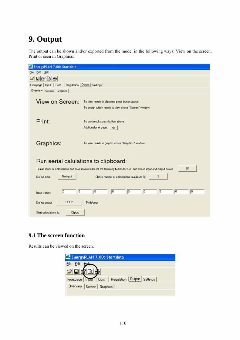
110

9. Output The output can be shown and/or exported from the model in the following ways: View on the screen, Print or seen in Graphics.

9.1 The screen function Results can be viewed on the screen.

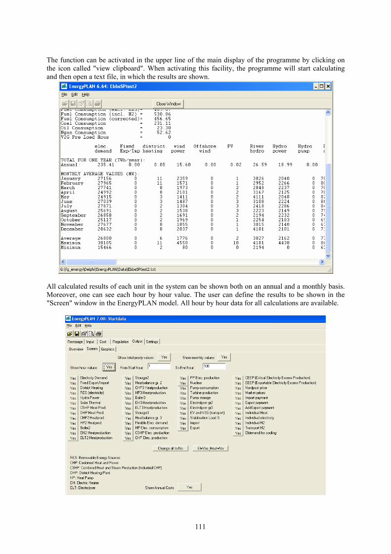
111

The function can be activated in the upper line of the main display of the programme by clicking on the icon called "view clipboard". When activating this facility, the programme will start calculating and then open a text file, in which the results are shown.

All calculated results of each unit in the system can be shown both on an annual and a monthly basis. Moreover, one can see each hour by hour value. The user can define the results to be shown in the "Screen" window in the EnergyPLAN model. All hour by hour data for all calculations are available.

112

9.2 The print Results can be printed in an A4 version defined by the model.

The function can be activated in the upper line of the main display of the programme by clicking the printer icon. When activating this facility, the programme will start calculating and then send a print to the printer. One can choose to add an additional page of specifications by clicking on “Yes” in the output overview window as shown below. In such case, two pages will be printed in stead of one.

Examples of prints are shown on the next page.

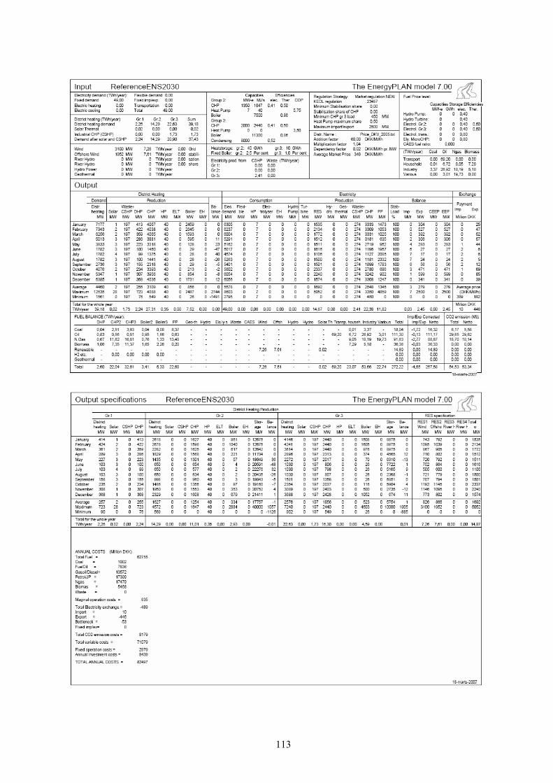
113

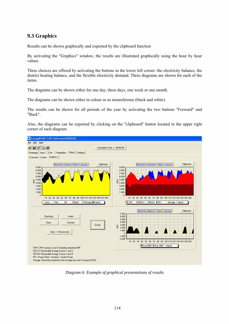
114

9.3 Graphics Results can be shown graphically and exported by the clipboard function By activating the "Graphics" window, the results are illustrated graphically using the hour by hour values. Three choices are offered by activating the buttons in the lower left corner: the electricity balance, the district heating balance, and the flexible electricity demand. Three diagrams are shown for each of the items. The diagrams can be shown either for one day, three days, one week or one month. The diagrams can be shown either in colour or as monochrome (black and white). The results can be shown for all periods of the year by activating the two buttons "Forward" and "Back". Also, the diagrams can be exported by clicking on the "clipboard" button located in the upper right corner of each diagram.

Diagram 6: Example of graphical presentations of results

115

9.4 Run serial calculations function

Moreover, the output window makes it possible to run series of up to 9 calculations by activating the “Run series calculations”. The calculations are started be activating either the “Clibrd” or the “Ascii” buttons. In the first case, the results are put into the clipboard and can be loaded into any Windows program such as Word or Excel by the Ctrl+V function. Before starting the series calculations, one has to - define which input parameters are to be changed by activating the “Define input” button - define how many calculations are to be carried out by activating the “series number” button - define a value of each input by writing inputs in the “input values” column, and - define which output parameter one wants to save in the Clipbrd/Ascii function by activating the

“define output” button. 9.5 Export Screen Data to Clipboard and e.g. EXCEL The same results which are shown in the screen function (defined by the user as described in section 9.1) can also be exported to the clipboard and thereby be loaded into e.g. EXCEL. This is simply done by setting the run serial button to “Off” and activating the clipboard function in the Output overview window:

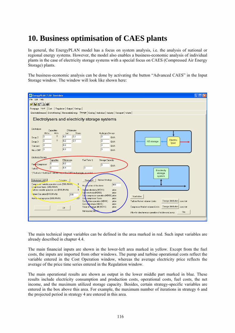
116

10. Business optimisation of CAES plants In general, the EnergyPLAN model has a focus on system analysis, i.e. the analysis of national or regional energy systems. However, the model also enables a business-economic analysis of individual plants in the case of electricity storage systems with a special focus on CAES (Compressed Air Energy Storage) plants. The business-economic analysis can be done by activating the button “Advanced CAES” in the Input Storage window. The window will look like shown here:

The main technical input variables can be defined in the area marked in red. Such input variables are already described in chapter 4.4.

The main financial inputs are shown in the lower-left area marked in yellow. Except from the fuel costs, the inputs are imported from other windows. The pump and turbine operational costs reflect the variable entered in the Cost Operation window, whereas the average electricity price reflects the average of the price time series entered in the Regulation window.

The main operational results are shown as output in the lower middle part marked in blue. These results include electricity consumption and production costs, operational costs, fuel costs, the net income, and the maximum utilized storage capacity. Besides, certain strategy-specific variables are entered in the box above this area. For example, the maximum number of iterations in strategy 6 and the projected period in strategy 4 are entered in this area.

117

In the upper part of the area marked in blue, one can choose between the following three operation strategies: - Strategy 4: Practical prognosis strategy - Strategy 5: Practical historical strategy - Strategy 6: Optimal Strategy (Theoretically optimal solution) Strategy 6 identifies the theoretically optimal strategy, i.e. the strategy which will identify the highest possible net operational income of a year given the specified input. The two other strategies represent practicable solutions. 10.1 Theoretically optimal strategy The methodology used for identifying the optimal operation strategy is the following: The key principle is based on the fact that in order to make a profit the market price of selling, Psell, has to be higher than the marginal cost of producing one unit of electricity, MCprod:

MCprod < PSell

The marginal production cost is defined by the marginal operations cost, the natural gas price and the price of buying electricity for the compressor. MCprod, is found by applying the following formula:

MCprod = PNgas * ηratio + MCt + [(Pbuy + MCc) / (ηc * ηt )]

In which - ηc is the compressor efficiency - ηt is the turbine storage efficiency defined as the power output per unit of energy storage input. - ηratio is the fuel ratio defined as the fuel input to the turbine per electricity output - MCc is the variable operational cost of the compressor - MCt is the variable operational cost of the turbine - PNgas is the natural gas price - Pbuy is the price of electricity for the compressor.

At some hours with very high electricity prices, it sometimes pays to bypass the storage while

operating the compressor and the turbine at the same time. Such operation is included in the strategy and allows the compressor and turbine to operate simultaneously during the same hour, in case the storage reservoir is empty.

The optimal operation strategy aims at finding the maximum theoretical operational income given a deterministic annual electricity price time series. The algorithm can be summarized by repeating the following 7 steps:

1) Identify the hour of the maximum electricity price (MAXhour) in the spot market price series.

Such hour is given priority when operating the turbine. (In the following iterations, hours already identified are disregarded and the hour of the remaining maximum price is picked).

2) Identify the storage boundaries around MAXhour. Running the turbine at MAXhour will have to

be compensated for by running the compressor in such a way that the storage boundaries are not compromised. In this step, the hours before and after MAXhour are examined. In the time period after MAXhour, the storage has to be charged before the storage reservoir is empty. Similarly, in the time period before MAXhour, the storage reservoir has to be charged after it is full. Consequently, the period between the last hour of full storage before MAXhour and the first hour of empty storage after MAXhour is identified. This range constitutes the time space in which

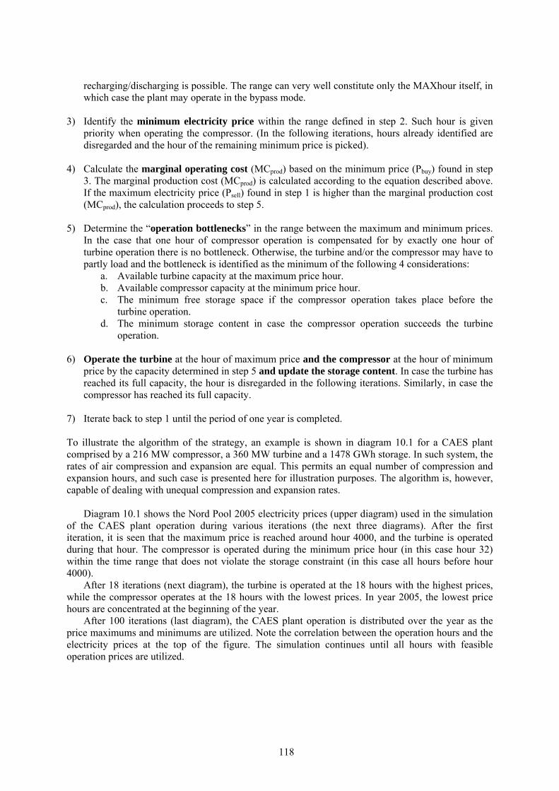
118

recharging/discharging is possible. The range can very well constitute only the MAXhour itself, in which case the plant may operate in the bypass mode.

3) Identify the minimum electricity price within the range defined in step 2. Such hour is given

priority when operating the compressor. (In the following iterations, hours already identified are disregarded and the hour of the remaining minimum price is picked).

4) Calculate the marginal operating cost (MCprod) based on the minimum price (Pbuy) found in step

3. The marginal production cost (MCprod) is calculated according to the equation described above. If the maximum electricity price (Psell) found in step 1 is higher than the marginal production cost (MCprod), the calculation proceeds to step 5.

5) Determine the “operation bottlenecks” in the range between the maximum and minimum prices.

In the case that one hour of compressor operation is compensated for by exactly one hour of turbine operation there is no bottleneck. Otherwise, the turbine and/or the compressor may have to partly load and the bottleneck is identified as the minimum of the following 4 considerations:

a. Available turbine capacity at the maximum price hour. b. Available compressor capacity at the minimum price hour. c. The minimum free storage space if the compressor operation takes place before the

turbine operation. d. The minimum storage content in case the compressor operation succeeds the turbine

operation. 6) Operate the turbine at the hour of maximum price and the compressor at the hour of minimum

price by the capacity determined in step 5 and update the storage content. In case the turbine has reached its full capacity, the hour is disregarded in the following iterations. Similarly, in case the compressor has reached its full capacity.

7) Iterate back to step 1 until the period of one year is completed.

To illustrate the algorithm of the strategy, an example is shown in diagram 10.1 for a CAES plant comprised by a 216 MW compressor, a 360 MW turbine and a 1478 GWh storage. In such system, the rates of air compression and expansion are equal. This permits an equal number of compression and expansion hours, and such case is presented here for illustration purposes. The algorithm is, however, capable of dealing with unequal compression and expansion rates.

Diagram 10.1 shows the Nord Pool 2005 electricity prices (upper diagram) used in the simulation of the CAES plant operation during various iterations (the next three diagrams). After the first iteration, it is seen that the maximum price is reached around hour 4000, and the turbine is operated during that hour. The compressor is operated during the minimum price hour (in this case hour 32) within the time range that does not violate the storage constraint (in this case all hours before hour 4000).

After 18 iterations (next diagram), the turbine is operated at the 18 hours with the highest prices, while the compressor operates at the 18 hours with the lowest prices. In year 2005, the lowest price hours are concentrated at the beginning of the year.

After 100 iterations (last diagram), the CAES plant operation is distributed over the year as the price maximums and minimums are utilized. Note the correlation between the operation hours and the electricity prices at the top of the figure. The simulation continues until all hours with feasible operation prices are utilized.

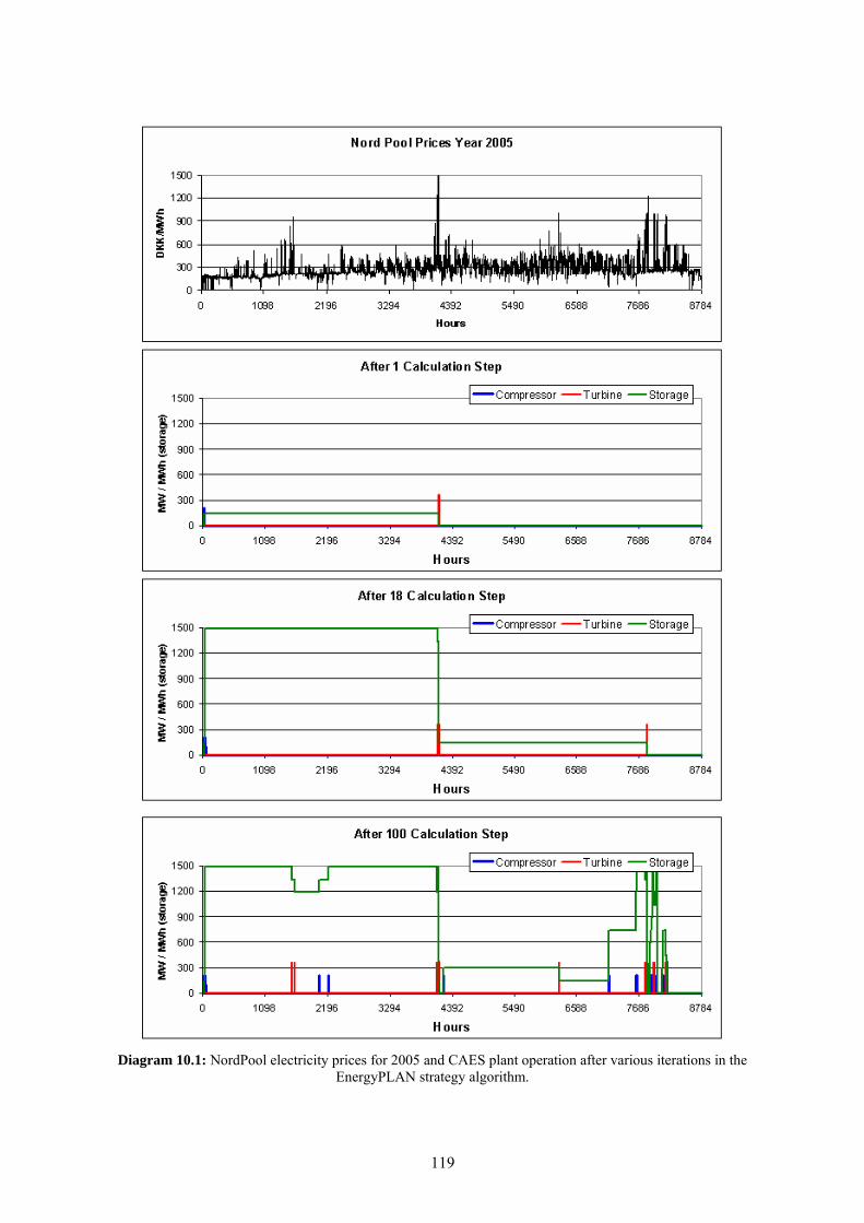
119

Diagram 10.1: NordPool electricity prices for 2005 and CAES plant operation after various iterations in the

EnergyPLAN strategy algorithm.

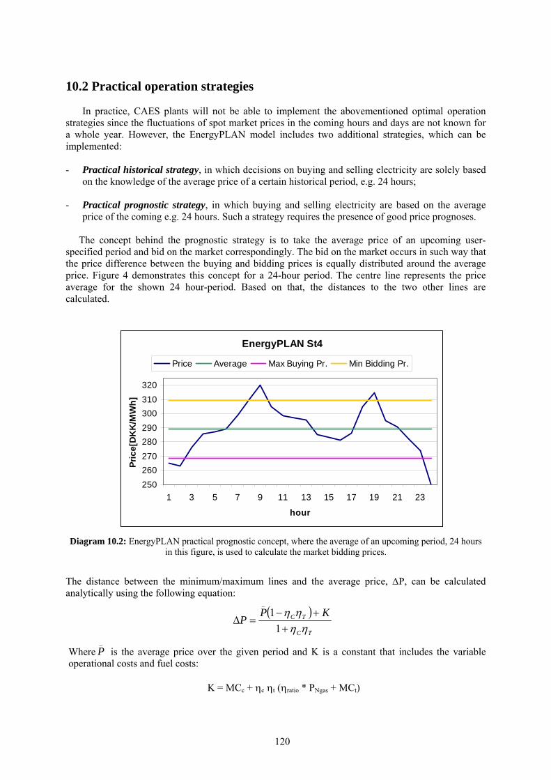
120

10.2 Practical operation strategies

In practice, CAES plants will not be able to implement the abovementioned optimal operation strategies since the fluctuations of spot market prices in the coming hours and days are not known for a whole year. However, the EnergyPLAN model includes two additional strategies, which can be implemented:

- Practical historical strategy, in which decisions on buying and selling electricity are solely based

on the knowledge of the average price of a certain historical period, e.g. 24 hours; - Practical prognostic strategy, in which buying and selling electricity are based on the average

price of the coming e.g. 24 hours. Such a strategy requires the presence of good price prognoses.

The concept behind the prognostic strategy is to take the average price of an upcoming user-specified period and bid on the market correspondingly. The bid on the market occurs in such way that the price difference between the buying and bidding prices is equally distributed around the average price. Figure 4 demonstrates this concept for a 24-hour period. The centre line represents the price average for the shown 24 hour-period. Based on that, the distances to the two other lines are calculated.

EnergyPLAN St4

250260270280290300310320

1 3 5 7 9 11 13 15 17 19 21 23

hour

Pric

e[D

KK

/MW

h]

Price Average Max Buying Pr. Min Bidding Pr.

Diagram 10.2: EnergyPLAN practical prognostic concept, where the average of an upcoming period, 24 hours

in this figure, is used to calculate the market bidding prices.

The distance between the minimum/maximum lines and the average price, ΔP, can be calculated analytically using the following equation:

( )TC

TC KPP

ηηηη

++−

=Δ1

1_

Where_P is the average price over the given period and K is a constant that includes the variable

operational costs and fuel costs:

K = MCc + ηc ηt (ηratio * PNgas + MCt)

121

It is noted here that the price average, _P , is a flexible average and is updated on an hourly basis,

as opposed to a fixed average over the specified period. This implicitly assumes the ability of the system operator to update market bids on an hourly basis. Again, the bypass of the storage at hours with very high electricity prices is included in the strategy, and allows the compressor and turbine to operate simultaneously during the same hour in case the storage reservoir is empty.

The practical historical strategy is similar to the prognostic strategy with the only difference that the average price is based on the previous 24 hours instead of a price prognosis for the upcoming hours.