r i k ’

Engineering Development of Slurry Bubble Column Reactor (SBCR) Technology

Quarterly Report

By: Bernard A. Toseland

Work Performed Under Contract No.: DE-FC22-95PC9505 1

For U.S. Department of Energy

Office of Fossil Energy Federal Energy Technology Center

P.O. Box 88.0 Morgantown, West Virginia 26507-0880

... BY

Air Products and Chemicals, Inc. 7201 Hamilton Boulevard !ihASTEB Allentown, Pennsylvania 181954-1501 .

Disclaimer

This report was prepared as an account of work sponsored by an agency of the United States Government. Neither the United States Government nor any agency thereof, nor any of their employees, makes any warranty, express or implied, or assumes any legal liability or responsibility for the accuracy, completeness, or usefulness of any information, apparatus, product, or process disclosed, or represents that its use would not infi-inge privately owed rights. Reference herein to any specifk commercial product, process, or service by trade name, trademark, manufacturer, or otherwise does not necessarily constitute or imply its endorsement, recommendation, or favoring by the United States Government or any agency thereof. The views and opinions of authors expressed herein do not necessarily state or reflect those of the United States Government or any agency thereof.

DISCLAIMER

Portions of this document may be illegible. in electronic image products. Images are produced from the best available original document.

ENGINEERING DEVELOPMENT OF SLURRY BUBBLE COLUMN REACTOR (SBCR) TEXHOLOGY

i Quarterly Technical Progress Report No. 3

for the Period 1 October - 31 December 1995

Contract Objectives The major technical objectives of this program are threefold: 1) to develop the design tools and a fundamental understanding of the fluid dynamics of a slurry bubble column reactor to maximize reactor productivity, 2) to develop the mathematical reactor design models and gain an understanding of the hydrodynamic fundamentals under industrially relevant process conditions, and 3) to develop an understanding of the hydrodynamics and their interaction with the chemistries occurring in the bubble column reactor. Successful completion of these objectives will permit more efficient usage of the reactor column and tighter design criteria, increase overall reactor efficiency, and ensure a design that leads to stable reactor behavior when scaling up to large diameter reactors.

Summary of Progress

State of the Art 0 A topical report on probes for the measurement of two- and three-phase flow was

reviewed and has been submitted to the DOE for review. . (Air Products and Washington University in St. Louis)

Technique Development 0 The precision of the CAFWT technique was improved by using wavelet filtering.

Wavelet filtering allows identification of the characteristic noise of the measurement process and subsequent filtering of this noise. Use of this technique on a test particle reduced the error in spatial resolution by at least 33% and by as much as 90% in some cases. The error in velocity measurement was reduced by at least 70%. In bubble- column measurements, errors in measurement of important hydrodynamic parameters such as Reynold's stresses and turbulent kinetic energy were significantly reduced by the use of filtering.

(Washington University in St. Louis)

The high-temperature, high-pressure bubble column'was tested. Pressures as high as 3000 psi were reached, and the capability of using solids and varying liquid velocity was demonstrated. Some misting after the pressure regulator must still be controlled, and flow rate is still limited by gas supply.

(The Ohio State University) Data Acquisition

Fundamental physical property data for two- and three-phase systems are not well understood, but are vital to understanding the fluid mechanics of such systems. Thus, a program of measuring properties such as interfacial tension and density has been

1

undertaken. Interfacial tension of N2/l?arathem NF was measured for pressures ranging from atmospheric to 3000 psig and temperatures of 27 and 56.5"C. Surface tension in the organic system shows the same decreasing trend with increasing pressure as do water/nitrogen systems.

(The Ohio State University)

0 The study of two-dimensional flow sometimes simplifies flow problems and leads to a more rapid understanding of the actual 3-D case. Thus, 2-D bubble columns were studied under a variety of flow rates using Particle Image Velocimetry (PIV). The PIV results revealed complicated flow structures that depend on gas velocity. A homogeneous flow regime, a regime containing four regions of flow, and a regime containing three regions of flow were seen as the velocity increased.

(The Ohio State University)

Model Development 0 A new phenomenological model for liquid flow has been proposed. The Recycle-

Crossmixing with Dispersion Model (RCFDM) augments the standard axial dispersion model (ADM) to allow for mixing at the top and bottom of the column and upflow and downflow regions in the column. The ADM alone cannot account for the tracer results seen at LaF'orte and in the laboratory. The RCFDM structure is such that it can account for the tracer results. The RCFDM fits the tracer patterns measured in the laboratory using independent CARPT measurements to fit parameters.

(Washington University in St. Louis)

Work on finding suitable closures for the Navier-Stokes equations for two- and three- phase flow continued. The major problem is finding suitable expressions for the interfacial momentum' exchange terms. Qualitative agreement for two-dimensional bubble columns is demonstrated using only a few terms--drag, virtual mass and mixing length for the Reynold's stresses.

(Washington University in St. Louis)

Data Processing Radioactive tracer data from the hydrodynamics trial were received. Qualitative analysis of the data revealed that the pre-trial planning was adequate, and good profiles have been obtained. The data have been transmitted to Washington University for analysis.

(Air Products and Chemicals)

2

The Ohio State University Research

The following report fiom Ohio State University for the period September-December, 1995 contains the following brief chapters:

1. Measurement of Interfacial Surface Tension between Liquid and Gas (Tasks 2-5) 2. Bubble Effects on the Transient Flow Pattern in Bubble Columns (Task 3) 3. High-pressure and -Temperature Slurry Column Shakedown (Task 2) 4. Work to be Performed Next Quarter (Task 7) 5. References

3

INTRI[NSIC FLOW BEHAVIOR IN A SLURRY BUBBLE COLUMN AT HIGH PRESSURE

AND HIGH TEMPERATURE CONDITIONS

(Quarterly Report)

(Reporting Period: October 1 to December 3 1,1995)

L. -S. Fan

DEPARTMENT OF CHEMICAL, ENGINEEFUNG THE OHIO STATE UNIVERSITY

COLUMBUS, OHIO 43210

January 14,1996

Prepared for Air Products and Chemical, Inc.

4

WORKPERFORMED

1, Measurement of interfacial surface tension between liquid and gas

An area of high pressure and high temperature operation of slurry bubble column systems

which is not fully understood is the effect of the physical property (densities, viscosity, surface

tension, etc.) of the gas and liquid phases on the transport phenomena as the pressure and

temperature increase. It may be possible to characterize the transport phenomena of slurry bubble

column systems operated at high pressure and high temperature based on the physical properties of

the phases rather than the operating pressure and temperature.

Slowinski et al. (1957) and Massoudi and King (1974) studied the pressure effects on the interfacial surface tension between the gas and liquid. Their results showed that the interfacial

surface tension decreases approximately linearly with increasing gas pressure. The extent of

reduction in the interfacial surface tension with pressure varies with the type of gas. The change in surface tension with pressure and temperature also depends on the liquid molecular structure and its

molecular weight. The surface tension of aliquid in equilibrium with its own vapor decreases with

increasing temperature in a low pressure system. Under high pressure conditions, the surface tension

tends to increase with increasing temperature for some liquid mixtures (Reid et al., 1977). Due to

the important role surface tension plays in the dynamic behavior of the bubble motion, it is necessary

to determine how the surface tension of various gas and liquid mixtures changes with pressure and

temperature.

A capillary probe developed last quarter was used to measure the interfacial surface tension

between Paratherm NF heat transfer fluid and nitrogen. The detailed design of the system was

described in the first quarterly report. The schematic diagram of the system is shown in Fig. 1.

Some modifications were done on the supporting rod after preliminary tests. A separate experiment was conducted to calibrate the capillary probe.

Interfacial surface tension varies with the absorption of nitrogen into Paratherm NF heat

transfer fluid. The interfacial surface tension was measured when the liquid is saturated with the

pressurizing nitrogen and liquid vapor. The measurements were carried out for pressures ranging from atmospheric pressure to 3000 psig, and temperatures of 27 and 56.5 "C. The experimental data

5

are shown in Fig. 2. As can be seen from Fig. 2, the surface tension decreases linearly with an

increase in pressure at both temperatures. f i e changes of the interfacial surface tension between

Paratherm NF heat transfer fluid and N2 with the pressure show the same trend as that of water - N2 system (Slowinski et al., 1957).

2. Bubble effects on the transientflow pattern in bubble columns

The experiment on transient flow structure in a two-dimensional bubble column under ambient conditions was carried out this quarter. The experiments focused on the identification of

the transient flow structure, and the relationship between the flow regimes (time-averaged

macroscopic behavior) and the transient flow structure. Two-dimensional systems were employed to yield important qualitative information in gas-

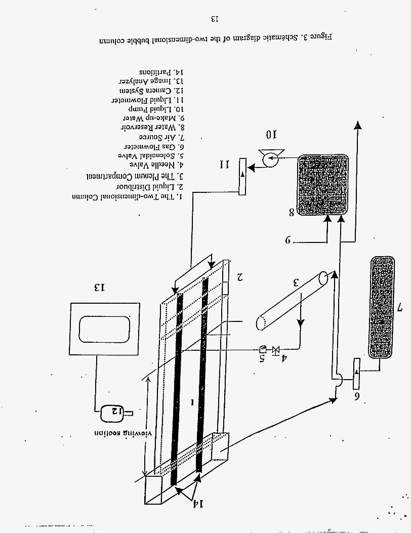
liquid systems. Figure 3 shows the schematic diagram of the experimental system. Two 2-D

columns made of transparent Plexiglass sheets have been used as the test columns. Column A is 48.3 cm in width, 1.27 cm in depth and 160 cm in height and consists of two movable partitions

between the Plexiglass sheets which allow the width of the bed to be varied. The viewing section

of Column B is 60.96 cm in width, 228.6 cm in height, and 0.64 cm in depth. Below the viewing

section is the gas distributor which consists of 0.016 cm I.D. tube injectors, flush mounted on the

column wall, 10 cm above the liquid inlet. The gas' through each injector is individually regulated

by a solenoid valve and a needle valve which are connected to the plenum compartment outside the

column. The distance between two adjacent bubble injectors is 5.08 cm and the distance fiom the end injector to the sidewall is 3.81 cm. When the width of Column A is changed, there is no liquid

and gas flow through the region outside the partitions.

Tap water was used as the liquid phase. The liquid phase was operated under batch

conditions for all studies. Neutrally buoyant Pliolite particles of 200-500 pm were used as the liquid

tracer. To ensure that the seeding particles follow the flow closely and have virtually no effects

on the flow structure, the concentration of the seeding particles was maintained around 0.1 % and

the Stokes number of the seeding particles was much smaller than 1. Air was used as the gas

phase. The gas pressure was maintained within 4 to 10 psig upstream of the gas plenum. The

superficial gas velocity ranges from 0.1 to 6.1 c d s . Acetate particles (4 = 1.5 mm, ps = 1250

6

..

kg/m3) were used as the solids phase in the study of slurry bubble column systems.

A high resolution (800 X 490 pixel) CCD camera equipped with variable electronic shutter

ranging from 1/60 to 1/8000 s was used to record the image of the flow field. A Particle Image

Velocimetry (PIV) system developed by Chen and Fan (1992) was applied to measure local flow

structures in the 2-D bubble columns. The PIV system is a non-intrusive technique which

provides quantitative results on a flow plane including instantaneous velocity distributions of

different phases, velocity fluctuations, gas and solid holdups, bubble sizes and their distributions,

and other statistical flow information.

Based on the macroscopic bubble flow behavior in bubble columns, three different flow regimes are commonly identified, Le. dispersed bubble, chum-turbulent and slugging (h4proyama

and Fan, 1985). A gross circulating flow of liquid is observed for these systems under both the

dispersed bubble and chum-turbulent (coalesced bubble) regimes (e.g., De Nevers, 1968;

Freedman and Davidson, 1969; Hills, 1974). In general, the gross circulation comprises an

upward flow in the central region and a downward flow along the wall with the inversion point

(zero axial liquid velocity) located at about 0.5 to 0.7 radius of the column (Walter and Blanch,

1983). This non-uniform velocity distribution is significant in characterizing the column

hydrodynamics, phase mixing characteristics, heat transfer and mass transfer. Based on the bubble

dynamics and local liquid flow patterns, Tzeng et aZ. (1993) found that when the gross flow

circulation occurs in the system, there are four distinct flow regions, namely central plume region,

fast bubble flow region, vortical flow region, and descending flow region, as shown in Figure 4.

The macroscopic flow behavior and flow regimes are directly linked to the transient flow

structure. Figure 5 shows a sample of the transient bubbling behavior in the dispersed bubble

regime and coalesced bubble regime. A homogeneous flow regime, a regime containing four

regions of flow, and a regime of containing three regions of flow are seen as the gas velocity is

increased in a 2-D bubble column. The dispersed bubble flow regime exists up to a gas velocity of 1 c d s . This regime is characterized by a relatively uniform gas holdup profile, uniform bubble

size and a rather flat liquid velocity profile. The bubbles in this regime are observed to rise

rectilinearly in the form of bubble streams. No coalescence or clustering of the bubbles in the

individual bubble streams or with adjacent bubble streams occurs. The liquid phase is carried

7

upward in the region of the bubble streams by the wake motion and the liquid drift effects

associated with the bubble motion. The liquid falls downward between adjacent bubble streams

with continuous dohward streams adjacent to the sidewalls. This descending motion of the liquid

coupled with the rising motion of the adjacent bubble stream generates small vortices in the liquid

streams between the rising bubble streams and the region adjacent to the sidewalls. The vortices

located adjacent to the sidewalls are observed to increase in size as the gas velocity increases in

the dispersed bubble regime due to the migration of bubbles away from the sidewalls. In this

regime, the induced liquid flow is dominated by the drift effects of the rising bubble streams. The 4-region flow condition exists for gas velocities between 1 and 3 cds . This condition

is characterized by a gross circulation of the liquid phase, wherein the liquid rises in the middle

portion of the column and descends adjacent to the sidewalls. The four flow regions (Figure 5 ) and the resulting flow phenomena were reported by Tzeng et al. (1993). In columns of width less

than 20 cm the central plume region becomes indistinguishable from the fast bubble flow region

yielding a 3-region flow.

The 3-region flow condition occurs at gas velocities greater than 1 c d s for small columns

(< 20 cm width) and at 3 c d s for larger columns (> 20 cm). In the 3-region flow condition the

two fast bubble flow regions merge together to form one central fast bubble region in the center

of the column. The gas flow in this regime is dominated by bubble coalescence and break-up.

The liquid flow is dominated by the wake effects from the large bubbles rising in the central part

of the column. The vortical flow region and descending flow regions are still observable. It is

noted that in a column of very small width, this flow commonly leads to the slugging condition.

3. High pressure and temperature slurry column shakedown A test run of the high pressure and temperature bubble column was completed this quarter.

It has been verified that the system can be operated at pressures up to 3000 psig. The liquid

velocity can be varied from 0 to 10 c d s at room temperature. Very high gas velocities can be

achieved depending on the gas cylinder's capacity and the duration of each test. It was found that

gas-liquid separation does work well. In this system, a single stage pressure regulator is used to

release the pressure from system pressure (up to 3000 psig) to the atmospheric pressure. The

8

liquid is atomized into fine droplets when it passes through the regulator. It is difficult to separate

these fine droplets in the exhaust reservoir.' We are still searching for solutions to this problem.

A test run of the system with addition of solids particles was also completed. It has been

verified that the system can be operated in a wide range of liquid velocity for completely particle suspension. Liquid-particle separation is achieved in the disengagement section.

WORK TO BE PERFORMED NEXT QUARTER

1. Experiments on transient flow structure in 2-D bubble column will be emphasized on the

column scale effects.

Measurements of interfacial surface tension will be continued next quarter in a system with

CO,. Measurements of liquid viscosity under high pressure and temperature will be

started.

2.

REFERENCES Chen, R.C., and L.-S. Fan, 1992, "Particle Image Velocimetry for Characterizing the Flow

Structure in Three-Dimensional Gas-Liquid-Solid Fluidized Beds, 'I Chem. Eng. Sci., 47,

3615.

De Nevers, N., 1968, "Bubble Driven Fluid Circulations," MChE J . , 14, 222.

Freedman, W., and J.F. Davidson, 1969, "Hold-up and Liquid Circulation in Bubble Columns,"

Trans. IChemE, 47, T251. Hills, J.H., 1974, "Radial Non-Uniformity of Velocity and Voidage in a Bubble Column," Trans.

IChemE, 52, 1.

Massoudi R., A. D. King, 1974, "Effect of pressure on the surface tension of water. Adsorption of low molecular weight gases on water at 25 OC," J. Phys. Chem., 78,2262.

Muroyama, K. , and L.-S. Fan, 1985, "Fundamentals of Gas-Liquid-Solid Fluidization, I' AIChE J. , 31, 1.

Reid, R. C., J. M. Prausnitz and T. K. Sherwood, 1977, The Properties of Gases and Liquids, McGraw-Hill, Inc. , New York.

9

Sl.owinski, E.R., E.E. Gates and C.E. Waring, 1957, "The effect of pressure on the surface tensions

of liquids", J. Phys. Chem., 61, 808-810.

Tzeng, J.-W., R.C. Chen, and L.4 . Fan, 1993, "Visualization of Flow Characteristics in a 2-D

Bubble Column and Three-phase Fluidized Bed," AIChE J., 39, 733. Walter, J.F., and H. W. Blanch, 1983, "Liquid Circulation Patters and Their Effect on Gas Hold-

Up and Axial Mixing in Bubble Columns," Chem. Eng. Commun., 19,243.

10

T- Liquid flow

m = liquid density pg = gas density

Figure 1. Schematic diagram of capillary tube surface tension measurement technique for high pressure systems.

11

I I I I I I

- Gas: nitrogen -

T=27 "C + T=56.5OC - -

- -

Figure 2. A preliminary study on the effects of pressures and temperatures on the surface tension of ParathermNF heat transfer fluid in N2

r

..

Free Surface

c___c

liquid or liquid-sc id flow

047 bubbles

t - - - - - bubble molion

Descending Flow Region

Fast Bubble Flow Region -

Central Plume Region

\ Vortical Flow Region

Figure 4. Classification of regions accounting for the macroscopic flow structures in 2-D bubble columns. .

14

Dispersed BubbIe Regime - Coalesced Bubble Regime (6region flow)

:*, .. .,.I . .. * ...*. ..-.

Coalesced ,Bubble Regime (3-region flow)

Figure 5 . Flow regimes in a two-dimensional bubble column

Washington University in St. Louis Research

The following report fiom Washington University for the period September-December 1995 contains the following brief chapters:

1. Introduction 2. Review of Measurement Methods (Task 1) 3. Interpretation of Tracer Runs at LaPorte (Task 4/Task 6) 4. Modification of CARPT-CT System for Slurry Bubble Column Studies (Task 3) 5. Phenomenological Model for Liquid Recirculation (Task 3) 6. CTDLIB Codes and Simulation (Task 3) 7. References

3 Q 9 5 . d ~ 16

.=.

Slurry Bubble Column Hydrodynamics

Third Quarterly Report for Contract DOE-FC 22-95 PC 95051

September - December, 1995

1 Introduction The main goal of the subcontract to the Chemical Reaction Engineering Laboratory (CREL) at Washington University is to study the fluid dynamics of slurry bubble columns and address issues related to scale-up. Experimental investigations to examine the effect of operating conditions such as superficial gas velocity, solids loading, type of distributor etc. on the fluid dynamics are to be made. The specific objectives that have been set out for the f i r s t year o f the project are as follows :

1. Assess the suitability of available experimental techniques for the measurement of global and some local hydrodynamic parameters in an industrial scale system and make recommendations for the use of these techniques at La Porte.

2. Interpret the existing tracer experiments and make recommendations for future tracer tests on La Porte reactor.

3. Modify the CARPT/CT experimental facility for study of slurry bubble columns.

4. Develop a phenomenological model for the key hydrodynamic features in bubble columns as a basis for an improved reactor model.

5. Introduce appropriate closure schemes and constitutive forms in the hydrodynamic codes to achieve agreements between data and models and test model reliability.

The activities that have been undertaken during the third quarter (September - December 1995) towards fulfilling the above mentioned objectives are described in the subsequent sections.

2 Review of Measurement Methods

This study has been completed and a summary of findings has been reported in the second quarterly report. A topical report on the subject entitled “Measurement Techniques for

17

Local and Global Hydrodynamic Quantities in Two and Three Phase Systems", has been submitted to Air Products.

3 Interpretation of Tracer Runs at La Porte

The reactor that was studied was the Alternative Fuels Development Unit (AFDU) at La Porte, Texas, which is a stainless steel bubble column reactor owned by D.O.E., with an internal diameter of 0.57 m and liquid height of 7.62 m. The slurry phase was powdered catalyst suspended in hydrocarbon oil. Gas was distributed via a sparger. For the cases considered thus far, the reactor temperature was 300" C, and pressure was 2.7 atm. The reaction was the dehydration of isobutanol to isobutylene and water. Due to complete conversion, the gas holdup was found to be almost doubled in the reactor.

Radioactive liquid and gas tracer measurements were made in the reactor. Ar-41, which is soluble in the liquid phase, was used as the gas phase tracer. Powdered manganese oxide was used as the liquid tracer since the particles were small enough to mimic the liquid flow. The distribution of the gas and liquid tracers in the column was monitored by four rings of four evenly distributed scintillation detectors, with an extra set of detectors at two other levels to monitor the gas distribution.

Since the tracers are radioactive, the signals measured by the scintillation detectors are affected by the solid angle subtended at the cylindrical detector, the distance between the radiation source and the detector, and other effects such as attenuation and buildup. These effects have been properly accounted for, the details for which are presented in Toseland et al., (1995). The normalized tracer curve that is finally obtained is taken to be linearly dependent on the tracer concentration. ,

The standard dispersion model was used to describe mixing in the liquid phase. For the gas phase, a dispersion model which included the solubility of Argon tracer was consid- ered. The following equations describe the gas and liquid mass balance for the tracer when interphase mass transfer resistance is also considered:

The following boundary and initial conditions were used :

18

.

!

-0 acG -0; -- z = L , -- 6% a2

. acL (4)

(5 )

It was assumed that the detector response is proportional to E L C L ( Z , ~ ) + E&’G(z,~).

More details of the model and the results are discussed in Toseland et. al. (1995). It was concluded that the liquid in the bubble column reactor was well mixed. However,

the axial dispersion model is not completely satisfactory for interpreting the gas phase tracer runs. Very high backmixing of the gas is indicated, but no conclusions can be reached regarding the flow pattern of the undissolved gas.

However, subsequent to this analysis, it was found that the detector levels reported by IC1 Tracerco were erroneous. In view of the corrections made, we are now in the process of reinterpreting the data using the existing dispersion model.

In addition to this, owing to the complex behavior observed in the bubble column reactor, and the asymmetric position of tracer injection points, it is proposed to use an alternative model, the Recycle with Cross-Flow and Dispersion (RCFD) model, that might be better suited to describing liquid mixing in the reactor. Details of this model are presented in a subsequent section. Work is also in progress on developing an alternative phenomenological model for gas tracer experiments.

4 Modification of CARPT-CT System for Slurry Bub- ble Column Studies

The planned studies of fluid dynamics in bubble columns required the following modifications in our CARPT-CT facility :

(i) Improvement of the accuracy of the CARPT technique in identifying radioactive par- ticle position and velocity using wavelet filtering. This was accomplished under the parallel DOE industry-university project “Novel Techniques for Slurry Bubble Column Hydrody- namics DEFG 22-95PC95212. Only the results pertinent to the execution of this contract are reported here.

(ii) Installation of pressure taps and pressure transducers dong the column in order to measure sectional pressure drops and dynamic pressure drop changes during the gas- disengagement method used for evaluation of bubble sizes.

(iii) Purchase and installation of a video camera for detection of the liquid level in the dynamic gas disengagement technique. This allows us to determine the modality of the

19

bubble size distribution at various flow conditions. (iv) Improved automatic calibration for CARPT is progressing in parallel as part of

(v) The possibilities of obtaining both liquid and solid velocities via CARPT are currently being studied as part of this program. If it proves feasible this will provide us with the needed information on solid-liquid slip velocities.

Below we will briefly describe the improved accuracy of CARPT obtained by wavelet filtering which is pertinent to this project. The wavelet filtering technique removes the intrinsic white noise (due to fluctuation in source emission) in the time versus instantaneous position data.

The statistical nature of the gamma radiation emitted from the particle gives rise to noise in the radiation intensity data and this gets transmitted to the position data. Wavelet analysis, a time-frequency based method, was identified as an appropriate method for ana- lyzing the nonstationary and localized data arising from CARPT experiments in multiphase systems.

To demonstrate its suitability in this regard, an experiment was conducted with a con- trolled motion of the radioactive tracer particle. This enabled a priori knowledge of the trajectory of the particle and provides a reference against which the results from CARPT experiments subject to wavelet packet filtering can be compared. A quantitative estimate of the errors involved in the estimation of the particle position, as well as the extent to which the intrinsic noise in the data is removed can therefore be arrived at: Thereafter the technique was applied to data from bubble column experiments.

DEFG 22-95PC95212.

4.1 Algorithm for filtering CARPT data using wavelet analysis

A brief outline of the algorithm used in the filtering procedure will be described here. For the sake of simplicity the mathematical details will be omitted. Wavelet packet decompo- sition using Daubechies’ orthonormal, nearly symmetric wavelets is employed for analysis. The algorithm consists of first transforming a set of data onto the wavelet packet domain, yielding a set of wavelet packet coefficients that contain the time-frequency (scale) content of the original data. The best basis representation of the coefficients is then obtained, by eliminating redundant coefficients. In the wavelet packet domain the coherent structures of the original signal are well represented by a few large coefficients while the incoherent part, that is basically the noise in the signal, is in the form of a large number of small coefficients. The wavelet packet coefficients (wpc) are therefore arranged in descending or- der of energy (energy Ewpc = up2). The first few significant coefficients correspond to the coherent part of the signal while the remaining weak coefficients depict the noise. The

20

.

coherent part is extracted by retaining the first few largest wavelet packet coefficients that possess an energy (E, = EES = &wpc2) equivalent to a fraction e of the total signal energy (Es = zzl wpc2). These coefficients are then re-ordered and reconstructed to yield the filtered signal. The weak coefficients (incoherent part) that remain are re-ordered and reconstructed to give the noise filtered. The tuning parameter in this algorithm is the en- ergy threshold E . This parameter is evaluated by conducting trial runs for a few data sets in the signal. Characteristics of white noise, such as the autocorrelation coefficient, are used as reference to select a proper threshold. Experiments show that the energy threshold is generally around 95 - 98% of the total signal energy. It is found that the results are insensi- tive to minor variations in the threshold value. Filtering using the above algorithm ensures maximum extent of reduction of the noise in the data, resulting in a smoother version of the signal and retains the sharp features arising from the na.ture of the flow in the system.

In order to verify the applicability and effectiveness of the algorithm for filtering noise from the data, the algorithm was tested with data produced from experiments for a controlled motion of the tracer particle.

4.2 Experimental setup The experimental setup principally consists of two motors, a screw conveyor and a plate as shown in Figure 4.1. Motor I is secured at the bottom of the structure and is geared to a screw conveyor that is positioned vertically. The screw conveyor supports a vertical frame on top of which the plate is mounted. The shaft of motor 11, which is fixed to the top of the plate, is connected to a smooth, circular disc. The radioactive particle to be tracked is fixed to the tip of a thin Plexiglas rod attached to the disc. Operation of motor I1 causes the particle to move in a circular motion. The maximum frequency of motion is 3 Hz. The distance of the particle from the center of radius varies from 7 to 8 cm. Simultaneously motor I causes the plate held to the frame to move vertically in “up and down” motion (with frequencies of the order of 0.1 Hz). The maximum vertical distance traversed by the particle is 6.4 cm. By this arrangement the particle is made to move in a spiraling 3D motion, with high (3 Hz) and low (0.2 Hz) frequencies. The two motors are driven by microprocessors, which are interfaced with a personal computer. A trolley system with guiding wheels provided for guiding the frame helps in minimizing the vibration of the setup. Calibration is first done using various particle positions that cover the entire range of experimental runs. Subsequently the experimental runs are performed. In each run, the speed of the two motors is varied, thereby varying the velocity of t.he particle. Eight such runs were performed.

A summary of the results for the entire set of runs is presented in Table 4.1 which reports

21

High frequency (3-5 Hz) motion

.particle

low frequency motion

*Stepper motor I

Figure 4.1 : Experimental setup for controlled motion of particle

the errors in position and spurious rms velocities, before and after filtering. It is evident by examining the results, that there is significant improvement in the accuracy of estimation of both the positions and velocities of the moving particle. The residual error (spurious rms velocities) after filtering the data is 2-5 cm/sec. There is an average of 75% reduction in the level of noise in the data. With regard to the magnitude of the rms fluctuating velocities of the liquid in bubble columns, which are an order of magnitude higher, the reduction in error is considered substantial.

4.3 Results for bubble column experiment We now show results for filtering of the data from a bubble column experiment. The exper- imental conditions for the run considered are : column diameter 19.05 cm, superficial gas velocity 3.2 cm/sec and superficial liquid velocity 0 cm/sec. The results presented in Figures 4.2, 4.3 and 4.4 are one dimensional profiles generated by averaging over the middle section of the column, where the flow is fully developed. As expected, there is no appreciable differ- ence between the filtered and original mean axial velocity profiles shown in Figure 4.2. This is because time averaging of the instantaneous velocities, averages all the fluctuations in the data, including the inherent noise due to statistical fluctuations of the radiation. Figures 4.3 and 4.4 show the turbulent kinetic energy and the Reynolds shear stress respectively. Here it can be seen that filtering has reduced the magnitude of these parameters. The data is

22

Table 4.1. Errors in Estimation of Particle Position (cm) and Velocity (cm/sec)

Run No. Direction Run 1 X

Y z

Run 2 X

Y z

Run 3 X

Y z

Run 4 X

Y z

Run 5 X

Y z

Run 6 X

Y

Run 7 X

Y

z

z Run 8 X

Y z

error in position, cm error in velocity, cm/sec Before Filtering After Filtering Before filtering After Filterin rms min/max rms min/max rms rms 0.32 -1.17,1.12 0.19 -0.7,0.6 20.5 4.16 0.36 -.15, 1.2 0.26 -0.75, 0.8 20.01 4.66 0.49 -1.7,1.4 0.25 -0.7,0.74 30.36 1.68 0.30 -1.23, 1.25 0.2 -0.76, 0.64 21.0 5.6

0.49 -1.6,1.6 0.2 -0.67,0.8 29.6 1.6 0.32 -1.16,1.13 0.21 -0.7,O.g 19.3 3.2 0.31 -1.2,1.2 0.21 -0.85,0.8 18.0 3.6 0.47 -1.5, 1.75 0.'17 -0.9, 0.6 28.9 1.34 0.32 -1.08,1.12 0.22 -0.75,O.M 19.5 4.8 0.32 -1.5,1.25 0.23 -0.7,0.75 19.0 4.5 0.46 -1.4,1.4 0.21 -0.65,0.61 29.0 1.38 0.3 -1.11,1.32 0.19 -0.9,0.66 20.2 5.4 0.29 -0.89,0.9 0.16 -0.61,0.65 18.7 3.8 0.47 -1.6,1.4 0.22 -0.87,0.72 29.2 1.56 0.32 -1.36,1.08 0.19 -0.55,0.52 20.9 6.3 0.29 -1.4,l.O 0.17 -0.68,0.7 19.11 . . 3.4 0.39 -1.42, 1.45 0.14 -0.64,0.32 26.1 1.01 0.31 -1.16,1.08 0.21 -0.8,l.O 19.78 4.18 0.28 -1.14,1.11 0.14 -0.84, 0.S2 18.69 3.51 0.37 -1.09,1.21 0.20 -0.86, 0.72 25.73 1.48 0.31 -0.97,1.03 0.03 -0.04,0.03 16.99 0.07 0.28 -1.10,1.15 0.007 -0.01, 0.02 17.94 0.04 0.40 -1.3,1.03 0.25 -0.79, 0.5 24.29 1.05

0.33 -1.43, 1.34 0.22 -0.79, 0.86 19.4 5.7

23

averaged over the middle section of the column where there appears to be negligible axial dependence of the parameters, and values are axially uniform. The profiles shown suggest that there is maximum turbulent shear and turbulent energy near the region of reversal in the flow direction. Comparison of the results for turbulent shear stress with data of Menzel et al. (1990), who used hot wire anemometry for measurement of the hydrodynamics, are shown in Figure 4.5. A good order of magnitude agreement is seen, which serves as an indirect verification of the results from CARPT for the turbulence parameters.

-Unfiltered data

20 - o o Filtereddata

0

P

-20 -

0 t I I I I I 1 I

1 2 3 4 5 6 7 8 9 -300

Radial Position, crn

Figure 4.2 : One dimensional mean axial liquid velocity for an 8" column, Uc 3.2 cm/sec

'5 Phenomenological Model for Liquid Recirculation The axial dispersion model (ADM) has been used in the past to fit the tracer response of multiphase reactors like bubble columns. In contrast to the computational fluid dynamics approach, which is directed at solving the complete transport problem in such reactors spatially and temporally, and involves massive computational power and problems of closure in the governing equations; phenomenological models are meant to be relatively simple, using a minimum number of adjustable parameters, and capture the essential features of the physics behind the backmixing in the system.

Models like the ADM and the tanks-in-series model are widely used in describing the mixing in flow systems, but are not found to be adequate in many instances, owing to the

24

I 1 I I 1 I 1

1 2 3 4 5 6 7 8 9 01 0

Radial Position, cm

Figure 4.3 : One dimensional turbulent kinetic energy for an 8" column, UG 3.2 cm/sec

Figure 4.4 : One dimensional Reynolds shear stress for an 8" column, UG 3.2 cm/sec

25

m I

Radial Position, cm

Figure 4.5 : Comparison of Experimental data for Turbulent Shear Stress from CARPT with Data of Menzel (Col. Dia. 14 cm)

fact that they describe mixing superimposed on unidirectional convective flow. It is well rec- ognized however (Hills, 1974; Devanathan et al., 1990) that in bubble columns there is both upflow of liquid (cocurrent with gas), as well as downflow of liquid (countercurrent with gas). Further, there is vigorous lateral mixing as well, in columns operating in the churn turbulent regime. Clearly then, it is not surprising that the ADM fails in many cases in describing the liquid mixing pattern. Notwithstanding such inadequacies in the model however, it continues to be extremely popular both in academia and the industry essentially because it is com- putationally simple with only one fitting parameter, and also because resolving the spatial dimensions further demands measuring mixing parameters experimentally, an undesirable alternative.

At CREL, the CARPT-CT facility allows us to measure the time-averaged liquid ve- locity profile, the backmixing parameters and the time-averaged gas-holdup distribution in the system. It was felt that this experimental knowledge could be used to overcome the inadequacies in previous models, such as the ADM, as pointed out above.

26

5.1 Model development: In the proposed model referred to as the Recycle-Crossmixing with Dispersion Model (RCFDM), the bubble column is divided axially into three sections, a middle zone and two end zones in which the liquid turns around (Fig. 5.1). The end zones are considered to be completely mixed, because it is not possible to resolve the complicated hydrodynamics in this region using a one-dimensional model. The middle zone is divided into two sections, one with the liquid flowing up in the core region, and another with liquid flowing down at the walls. In

x=L

x-0

F,GI ‘ Figure 5.1: Schematic Diagram for Recirculation and Cross Flow with Dispersion (RCFD) Model

this way the radial variation of liquid flow is lumped into two parts. The flow within each of these sections is considered 1-0 be in the middle region of the bubble column where the flow is assumed to be fully developed (an assumption based on the experimental observations of the liquid flow patterns obtained from CARPT in our laboratory).

Superimposed on the convective recirculation is the mixing caused by random turbulent fluctuating motion of the fluid elements, caused by the wakes of the rising bubbles, which give rise to axial dispersion as well as radial exchange between the two sections. Turbulent axial mixing is accounted for by an axial dispersion coefficient in each section, and radial mixing is incorporated by an exchange coefficient between section 1 and section 2.

Based on the above assumptions, the model equations may be formulated as follows. For the upflow region:

a2c, - ac, li’ u1- - -(C1- C2) ac1 -= --

at D l a x 2 ax A~

27

where K is the exchange coefficient (cm2/s) between the upflow and downflow sections, D1 is the dispersion coefficient in the upflow region (section 1) based on. the liquid covered cross-sectional area, and, €1, Cl, and AI are the average liquid holdup, velocity and cross sectional area of the upflow section.

Similarly, for the downflow region:

a2C2 aC1 K a~ A2

-- + ii2- + -(C1 - C2) - 0 2 - at d X 2 ac2

(7)

The equations for the well mixed regions, A and B which are assumed to connect the ends of the recirculating sections, are, respectively:

where Fo is the inlet liquid volumetric flowrate to the column, Fl, F2, Fa and Fb are the liquid volumetric flowrates in the upflow section 1, downflow section 2, region A and region B respectively. Initial conditions for a step input of tracer at the bottom of the column are:

Boundary conditions for the upflow region are given by equations (6) and (7) and for the

For the upflow section: downflow region by equations (8) and (9), as follows.

For the downflow section;

The above model requires as inputs the input function of tracer, the dimensions of the column (Table 5.1), the average upflow and downflow liquid interstitial velocities, and the average holdups in the different sections of the column.

28

Table 5.1 Operating Conditions for Tracer Experiments

Diameter of Column

Height of Column

Sup. Gas Velocity Us Sup. Liquid Velocity Ur Mean Residence Time of Liquid

Mean upflow velocity, 3 Mean downflow velocity, 4 Mean liquid holdup in upleg E;' Mean liquid holdup in downleg E;

-

19.0 cm

2.44 m

10.0 cm/s

1.0 cm/s

3.25 min

12.5 cm/s

7.7 cm/s

0.792

0.88

The experimental information was obtained from the CARPT-CT facility, from which the mean liquid velocities are calculated from the cross-sectional averaging of the recirculating liquid velocity profile (CARPT) (Fig. 5.2(a)) and the holdup profiles (CT) (Fig. 5.2(b)).

The model equations were solved numerically using implicit finite differences with back- ward differences in spatial coordinates. Implicit method was necessary because of the nature of the boundary conditions, and appropriate discretization was required for accurate conver- gent results. Solution of the model equations results in the F-curve, which on differentiation yields the Ecurve.

The heights of the two well-mixed regions A and B are assumed to be equal to the diameter of the column, an assumption based on observation of churn-turbulent bubble columns. However, it was found on running the simulation that the model is insensitive to the volumes of these sections.

5.2 Results and discussion: The objectives in developing this model were twofold: first, we wanted to develop a model which, based on the physics, would in general perform better for churn-turbulent bubble columns than existing models. Secondly, we wanted to see if given the experimental obser- vations from CARPT-CT, whether it would be possible to predict the RTD to a reasonable extent.

29

a 3 0- -I -

Radial Position, cm (4 ,

4 s 0

a 3

3"

1 .o

.9 *

-7 0 .2 -4 .6 .E 1.0

Nondimensional Radius @I

Figure 5.2: Azimuthally, Axially and Time.Averaged (a) Liquid Axial Velocity Profile, (b) Liquid Holdup Profiles

As a comparison of the models, the ADM, the recycle with crossmixing and the present model (RCFDM) were used to fit the experimental data (Fig. 5.3).

1 .o

.E

.6

wo

.4

2

0 0 1 2 3

Dimensionless l ime, 8

Figure 5.3: Measured RTD of an Experimental Bubble Column versus Model Predictions

1.0

8

.6

w" 4

2

0 0 1 2 3

Dimensionless l ime, 8

Figure 5.4: RCFD Model Predictions Based on Parameters Estimated from CARPT Data

The model parameters thus obtained in each case are shown in Table 5.2. Also shown is the sum of square of errors, which is found to be minimum,in the present case.

An independent assessment of the model parameters was attempted using the experi- mental data from CARPT. From CARPT, an estimate of the axial dispersion coefficients can be obtained by spatial averaging of the measured axial eddy diffusivities in the upflow and downflow sections, respectively. The average value of the radial eddy diffusivity at the

30

w i

Model

RCFDM ADM Recvcle-Crossflow

1 .O i -

*.-.* V, = V, = 6270 cm3 *--* v, = v, = 4702.5 cm3

0 1 2 3 4 5

Fitted/Predicted* Parameter e2

D1 = 113~m~/s,Di = 113cm2/s, k = 69cm2/s 0.0366 D,fj = 2 5 7 . 5 ~ ~ ~ ~ 1 ~ 0.0403

IC = 30.37 cm2/s 0.132

Dimensionless Time. 0

Figure 5.5: Effect of Entry and Exit CSTR Volumes on Prediction of RCFD Model

L m

0

T i e . s

Figure 5.6: RCFD Model Prediction . of Response to an Impulse Injection (D = 19 cm, U, = 2cm/s, Ut = 0 cm/s)

RCFDM from CARPT' I D1 = 285cm2/s,D1 = 440cm2/s, IC = D,,., = 4 3 ~ 2 / ~ I 0.0724 ~

point of inversion is taken as the crossmixing coefficients between the two legs. The RCFDM prediction using these parameters (Table 5.2) is shown in Fig. 5.4. This exercise seems to predict the tracer response independent of any experiment, based on the knowledge from the hydrodynamics .

Figure 5.5 shows that changing the volumes of the inlet and exit well mixed zones has no appreciable effects on the predicted tracer response. However, including them in the model renders the computations stable and does not lead to sharp fronts at the inlet and exit.

Since the RCFDM, using parameters estimated from CARPT results, is able to match well the observed tracer response (Fig. 5.4), we proceed to study the mixing behavior for batch liquid, in a 19 cm diameter column of expanded liquid height 65 cm, at a superficial gas velocity Us = 2cm/s. A pulse injection into the region A is simulated, using the batch version of t,he RCFDM. Figure 5.6 shows the resulting tracer concentrations as a function of time, at different axial locations in the column. As expected from the physics of t.he

31

problem, there are instants of offshoots in the upflow section of the column where the tracer moves up initially by convection. Although these predictions look quite realistic, they need to be confirmed by additional tracer experiments. Needless to say, ADM or any other one dimensional model cannot predict such a variation in the dynamics in different parts of the system.

5.3 Future work:

The lack of fully quantitative agreement between the RCFDM and CARPT data can be attributed to the fact that as it currently stands, the model does not consider the radial variation of liquid velocity and holdup profiles, but takes into account only the average flow

in each section. Hence, the axial dispersion coefficient in each section does not directly correspond to the axial eddy diffusivities but also accounts for the contribution from the radial variation of axial liquid velocity. The relationship between CARPT measurements and the RCFDM parameters need to be further developed based on additional analysis, which is in progress.

One needs to develop some independent means of predicting at least the average upflow and dowdow velocities either through theory or through simple experiments, because one cannot be expected to make CARPT runs at all industrial setups for which the use of the RCFDM is intended.

The model will be modified for predicting the tracer response of reacting systems in which gas may be evolved, causing a significant axial variation in holdup because of reaction (such as in the runs made at AFDU, La Porte, Texas). For this the equations have to be modified

!

32

1 I .

for predicting the response of radioactive tracer through detectors placed at the wall (since each detector spans a solid angle).

Finally, the expressions for interphase mass transfer will be incorporated into the model to incorporate the effect of soluble gas. The ultimate idea should be to develop a single physics-based phenomenological model which is able to predict the response of both gas and liquid phase tracer.

6 CFDLIB Codes and Simulation The Computational Fluid Dynamics Library (CFDLIB) code was developed at Los Alamos National Laboratory (LANL) under a CRADA agreement between Amoco Oil R & D and LANL. Being a sponsor of the Chemical Reaction Engineering Laboratory (CREL), Amoco granted CREL the privileges of using the CFDLIB code. The CFDLIB codes are capable of simulating three dimensional, multiphase, multispecies flows. Possibilities for including

,

chemical reactions exist. Here we report a test case for a gas-liquid flow problem that has been simulated. For

this simulation the experimental conditions of Chen et. al. (1989) were considered. In their experiments the gas-liquid flow in a two dimensional bubble column was studied using flow visualization techniques. The experiment was conducted at several L/D ratios of the dispersion and in all the cases Chen et. al. (1989) observed the formation of a series of well defined counter rotating circulation cells in the flow. The geometry simulated is a two dimensional bubble column with a width of 11 cm and three of the L/D ratios used by Chen et. al. were simulated. The superficial gas velocity was 0.035 m/s. Figure 6.1 shows the computed flow fields at one instant of time (approximately 90 seconds after start up) and it can be seen that the code is able to predict the experimentally observed circulation cells at all the three L/D ratios. The most important factor in the simulation of multiphase flow using a CFD code is in the choice of the interfacial momentum exchange terms. For this particular simulation the effects of drag, lift and virtual mass were used. The turbulence effects were modeled using the mixing length approach. The models for closure of these terms were as follows:

0 Drag is expressed as

0 Virtual mass effects are expressed by

33

0 Mixing length model is used for turbulence closure

A constant bubble size was used in the simulation and the value of CD was set to 0.44 since the particle Reynolds number turns out to be in the inertial range. C, - the coefficient in the virtual mass model was set to the standard value of 0.5. The mixing length scale was set to 1.5 cm and this value was arrived by trial and error based on the observed flow pat tern.

Currently, the code is being benchmarked against a wide range of multiphase flow prob- lems for which experimental or simulated results are available in the literature. Specifically efforts are being directed towards gas-liquid flow systems (bubble columns) under operating conditions for which experimental results have been obtained using the CARPT-CT system in our laboratory.

7 References

Chen, J. J. J., Jamialahmadi, M. and Li, S. M., 1989, Effect of Liquid Depth on Circulation in Bubble Columns, Chem. Eng. Res. Des., Vol. 67, pp. 203-207.

Devanathan, N., Moslemian, D.*and Dudukovit, M. P., 1990, Flow mapping in bubble columns using CARPT, Chem. Engng. Sci., 45, 2285.

Hills, J. H., 1974, Radial nonuniformity of velocity and voidage in a bubble column, Trans. Inst. Chem. Engng. 52, 1-9.

Menzel, T., T. in der Weide, 0. Staudacher, 0. Wein and U. Onken, ‘Reynolds Shear Stress for Modeling of Bubble Column Reactors’, Ind. Eng. Chem. Res., Vol. 29, 988-994 (1990).

Toseland, B. A., Brown, D. M., Zou, B. S. and Dudukovik, ‘Flow Patterns in a Slurry Bubble Column Reactor under Reaction Conditions’, Trans. I. Chem. E., 73(A), 297 - 301.

34

f

r

c l-i 0 0

al rl

s

0 P r

I I

3 0 0

E 0 rl U lu rl

c z

i$ cn

.. 4 . QI k 1 M z o o

4 ..

0 m

0 c\I

II

n n A A u co I-z 35

Task 4/Task 6 Data Processing for SCBR Tracer Runs

Tracer Studies I

Introduction As discussed in the last quarterly report1 a series of tracer studies has been carried out using the DOE AFDU at LaPorte. This section describes the results of the most recent (June 1995) tracer studies. The results are presented in the form of graphs which illustrate the resolution of the various issues in the trial. A more quantitative report will be written when the mathematical analysis of the residence t i e distribution studies is completed at Washington University.

Plant Trial Results Planning for the trial was discussed in the last report. A series of technique improvements and operating procedures was proposed for the trial based on our previous experience. These issues are discussed below:

a. Calibration ' Seven rings of four detectors were placed on the column. The previous practice was to calibrate the detectors to each other, detector ring by detector ring. No attempt was made to relate the calibration for one ring to that of the another. We requested that all detectors be calibrated on the ground. Unfortunately, for the present time, the results were reported based on the old calibration method. A calibration chart is available for each detector so that the values can be readjusted at a later date. A potential issue is that the response of a detector is related to the length of electric cable attached. Thus, the best calibration results when the detector-cable pair are calibrated together. This will be requested next trial. An example of the problem caused by ring-by-ring post- calibration is shown in Figures 1 and 2.

Aside from the differences caused by the changes in holdup with height, the radiation level in the column should be equal, and all of the traces should converge to a single point for long periods. As shown in Figure 1, the final intensity varies over the height of the column. This variation is apparently not correlated to height or holdup profile. As shown in Figure 2, all of the data converge for a single ring, but the intensity differs greatly for even adjacent rings. As indicated above, the calibration data for each detector exists and, thus, a first-order correction can be made when the calibration factors are obtained &om Tracerco.

IEngineering Development of Slurry-Bubble-Column Reactor (SCBR) Technology

36

350 - 300 - 250 - 200 - 150 - 100 - 50 -

lntensit j

Figure 1 Intensify Proceeding Up South Side of Reactor

height 338

:::.

0 100 200 300 400 500 600

Time, sec.

37

0

Figure 2 Intensity for Two Consecutive Rings of Detectors

I 1 I 1 I 1 I 1

0 100 200 300 m 5 0 0 ' 6 M )

Time, seconds I-

b. Gas Recycle Some unreacted syngas is recycled to the reactor. The recycle stream will contain some of the tracer gas and, thus, cause a second pulse through the column. Preliminary calculations indicated that the residence time in the recycle loop should be 5-10 minutes. It was judged that the system would have returned to baseline bythis time so that the recycle should not affect the initial residence time distribution (RTD) measurements.

As shown in Figure 3, a second peak is seen starting at about 5 minutes after the initial injection. The original radiation pulse shows a return to baseline, confinning the judgment made in the planning process that the recycle would not affect the RTD measurements. The peak is long and extends over a long period, indicating that there is extensive mixing in the recycIe section as anticipated.

38

Figure 3 Typical Gas Phase Profiles

I I 1 I 1 I 1 1

lime, sec. ,011

0 100 m 300 400 500 600

c. Liquid Phase Pso9les Typical radiation profiles for an injection at the side of the column are shown in Figures 4 and 5. Figure 6 shows a typical response for an injection in the center of the column.

39

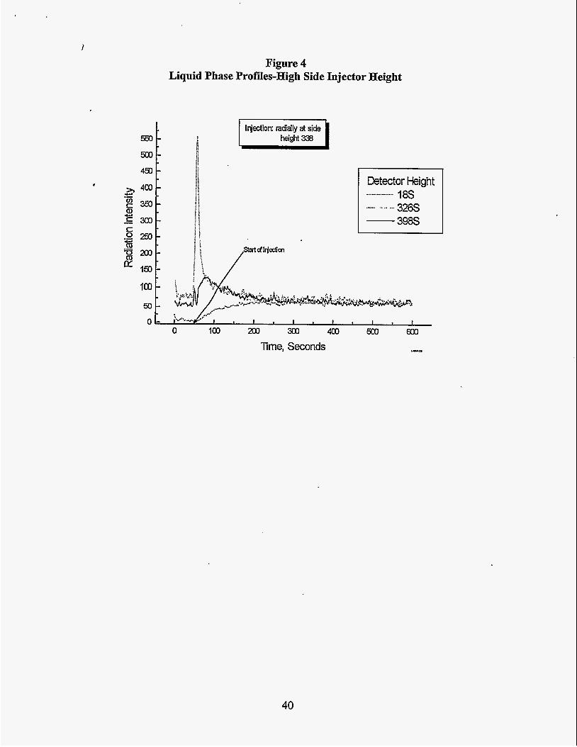
Figure 4 Liquid Phase Profiles-High Side Injector Height

Iqection: mdially at side

450

4(30 .- 27 .. .. .. .. .. .. .. .. .. .. .. .. . . . . s300 + PI ..

Detector Height

............. 32% .. . . . . . . . . . . . . . . . . . I . . . . . .

S .o 250 - 4-4

0 100 200 300 403 500 600

Time, Seconds I__

40

m

150

50

0

Figure 5 Liquid Phase Profiles- Side Injection, Lower Nozzle

I I height 98 Injection: radially at side

Detector INJECTION 18N 86N

................... -- - 398N

41

Figure 6 Liquid Phase Profiles- Low Center Injector Height

height 93 Detectors

INJECTION 18N 86N 398N

.... - ........... ”

----_---___

1 1 I 1 1 1 I I

0 100 200 300 400 m 600

lime, Seconds *-E.

Standard profiles which one would expect from an axial dispersion model are developed far away from the injector-for the detector at 18 for the high injection(338) and for the detector at 398 for the low injection(98). However, the profles near the injection point are distorted by time- averaged motion of the eddies in the column. Further evidence of the time averaged convective motion can be seen in Figures 7 and 8.

42

Figure 7 Upward Flow at the Center

Injection: Center

n Detectors ___-_______ ..-.. " ............ 1 !Y!N ,

INJECTION

0 103 200 300 400 5(x3 600

lime, Seconds .-I.

The detectors immediately above and below the injection point show a sharp spike of radiation immediately after injection. This is an indication that part of the injection is swept upward by upflowing eddy, while part is swept downward by a d o d o w i n g eddy. Note that the upflow pulse is much stronger, as would be expected for the central region where the time-averaged flow is upward.

The time-averaged flow at the wall is downward. As can be seen from Figure 4, there is a strong pulse down the column for the side injection, indicating the predominance of average down flow at the wall. Only a small amount of material travels up the column, in this case where the tracer is injected at the side of the column. It should be noted that the injectors were fixed to inject horizontally at the wall, not downward as in the previous trial. Thus, we conclude that the tracer experiment provides good evidence of strong downflow at the Wall.

Since there is strong turbulence in the process, sometimes the flow can be seen to be almost evenly split in the pulse up and down the column. This is shown in Figure 8 for a center injection. However, for most liquid tracer runs, the predominant flow is up in the center and down at the wall. This means that the standard one-dimensional dispersion model is not physically based for bubble column flow. Lack of a physical basis implies poor scaleup capability. A new model is being developed by Professor Dudukovic's group at Washington University.

43

Figure 8 Liquid Upflow and Downflow at the Injection Point

Height 98 I Detect o IS

INJECTION 8 6 N 1 ION

". .-. .... - .... __________-

I I I I 1 1 I 1 I

0 100 m 3M3 4co 500 600

Time, Seconds .- d Gas Phase Tracer Results Gas phase results look good. Typical gas phase profiles have been shown in Figure 3. Gas phase results appear the same as for previous trials.

A good, sharp initial pulse was obtained. The profiles widen as the radiation pulse moves up the column. A substantial part of the widening takes place before the fist set of rings. As in the last tracer study, this is attributed to some CSTR-like mechanism in the very bottom of the column.

The time-of-arrival of centroid of the pulse increases as it moves up the column. The tirne-of- arrival of the centroid is longer than that expected from a calculation based on the average superficial gas velocity (calculated as t = Ugkg, where Ug is the superficial gas velocity and E is the void fraction). As in the previous tracer study, this is attributed to the solubility of the tracer gas in the process fluid, causing a delay in the time of arrival. Thus, we anticipate that a version of the axial dispersion model that accounts for gas solubility will have to be used for analysis.

44