enzyme kinetics - university of ottawa · experimental kinetics! 5! practical kinetics 1....
TRANSCRIPT

CHM 8304
Experimental Kinetics 1
Enzyme Kinetics
Experimental Kinetics
Outline: Experimental kinetics • rate vs rate constant • rate laws and molecularity • practical kinetics • kinetic analyses (simple equations)
– first order – second order – pseudo-first order
• kinetic analyses (complex reactions) – consecutive first order reactions – steady state – changes in kinetic order – saturation kinetics – rapid pre-equilibrium
see A&D sections 7.4-7.5 for review
2

CHM 8304
Experimental Kinetics 2
Rate vs rate constant
• the reaction rate depends on the activation barrier of the global reaction and the concentration of reactants, according to rate law for the reaction – e.g. v = k[A]
• the proportionality constant, k, is called the rate constant
3
Rate vs rate constant • reaction rate at a given moment is the instantaneous slope of [P] vs time • a rate constant derives from the integration of the rate law
0
10
20
30
40
50
60
70
80
90
100
0 5 10 15 20
Temps
[Produit]
different initial rates
same half-lives; same rate constants
different concentrations of reactants; different end points
4

CHM 8304
Experimental Kinetics 3
Rate law and molecularity • each reactant may or may not affect the reaction rate, according to the
rate law for a given reaction • a rate law is an empirical observation of the variation of reaction rate as
a function of the concentration of each reactant – procedure for determining a rate law:
• measure the initial rate (<10% conversion) • vary the concentration of each reactant, one after the other • determine the order of the variation of rate as a function of the concentration of
each reactant • e.g. v ∝ [A][B]2
• the order of each reactant in the rate law indicates the stoichiometry of its involvement in the transition state of the rate-determining step
5
Integers in rate laws
• integers indicate the number of equivalents of each reactant that are found in the activated complex at the rae-limiting transition state – e.g.:
• reaction: A + B à P – mechanism: A combines with B to form P
• rate law: v ∝ [A][B] – one equivalent of each of A and B are present at the TS of the rds
6

CHM 8304
Experimental Kinetics 4
Fractions in rate laws
• fractions signify the dissociation of a complex of reactants, leading up to the rds: – e.g. :
• elementary reactions: A à B + B; B + C à P – mechanism: reactant A exists in the form of a dimer that must dissociate before
reacting with C to form P
• rate law: v ∝ [A]½[C] – true rate law is v ∝ [B][C], but B comes from the dissociation of dimer A – observed rate law, written in terms of reactants A and C, reflects the dissociation of A – it is therefore very important to know the nature of reactants in solution!
7
• negative integers indicate the presence of an equilibrium that provides a reactive species: – e.g. :
• elementary reactions: A B + C; B + D à P – mechanism: A dissociates to give B and C, before B reacts with D to give P
• rate law: v ∝ [A][C]-1[D] – true rate law is v ∝ [B][D], but B comes from the dissociation of A – observed rate law, written in terms of reactants A and D, reflects the dissociation of A – apparent inhibition by C reflects the displacement of the initial equilibrium
Negative integers in rate laws
8

CHM 8304
Experimental Kinetics 5
Practical kinetics
1. development of a method of detection (analytical chemistry!) 2. measurement of concentration of a product or of a reactant as a function
of time 3. measurement of reaction rate (slope of conc/time; d[P]/dt or -d[A]/dt)
– correlation with rate law and reaction order 4. calculation of rate constant
– correlation with structure-function studies
9
Kinetic assays
• method used to measure the concentration of reactants or of products, as a function of time – often involves the synthesis of chromogenic or fluorogenic reactants
• can be continuous or non-continuous
10

CHM 8304
Experimental Kinetics 6
Continuous reaction assay
0
10
20
30
40
50
60
70
80
90
100
0 5 10 15 20
Time
[Pro
duct
]
Continuous assay • instantaneous detection of reactants or products as the reaction is
underway – requires sensitive and rapid detection method
• e.g.: UV/vis, fluorescence, IR, (NMR), calorimetry
Continuous reaction assay
0
10
20
30
40
50
60
70
80
90
100
0 5 10 15 20
Time
[Pro
duct
]
11
Continuous reaction assay
0
10
20
30
40
50
60
70
80
90
100
0 5 10 15 20
Time
[Pro
duct
]
Discontinuous assay • involves taking aliquots of the reaction mixture at various time points,
quenching the reaction in those aliquots and measuring the concentration of reactants/products – wide variety of detection methods applicable
• e.g.: as above, plus HPLC, MS, etc.
12
Continuous reaction assay
0
10
20
30
40
50
60
70
80
90
100
0 5 10 15 20
Time
[Pro
duct
]
Discontinuous
CHM 8304
Experimental Kinetics 7
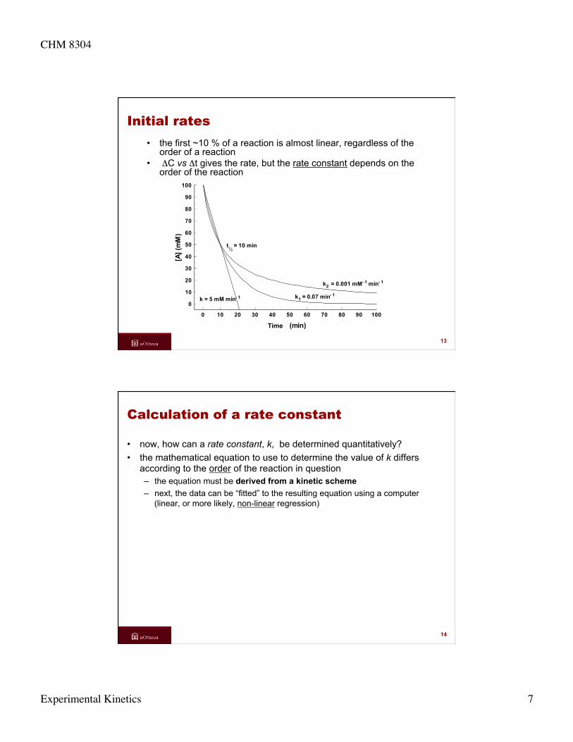
Initial rates • the first ~10 % of a reaction is almost linear, regardless of the
order of a reaction • ΔC vs Δt gives the rate, but the rate constant depends on the
order of the reaction
0 10 20 30 40 50 60 70 80 90 100
Temps (min)
0
10
20
30
40
50
60
70
80
90
100[A
] (m
M)
k = 5 mM min- 1 k1 = 0.07 min- 1
k2 = 0.001 mM- 1 min- 1
tΩ = 10 min
Time
13
½
Calculation of a rate constant
• now, how can a rate constant, k, be determined quantitatively? • the mathematical equation to use to determine the value of k differs
according to the order of the reaction in question – the equation must be derived from a kinetic scheme – next, the data can be “fitted” to the resulting equation using a computer
(linear, or more likely, non-linear regression)
14

CHM 8304
Experimental Kinetics 8
Outline: Kinetic analyses (simple eqns)
– first order reactions – second order reactions – pseudo-first order – third order reactions – zeroth order
15
The language of Nature • “Nul ne saurait comprendre la nature si
celui-ci ne connaît son langage qui est le langage mathématique”
- Blaise Pascal – (‘None can understand Nature if one does not know its
language, which is the language of mathematics’)
• Natural order is revealed through special mathematical relationships
• mathematics are our attempt to understand Nature – exponential increase: the value of e – volume of spherical forms: the value of π
Blaise Pascal, French mathematician
and philosopher, 1623-1662
16

CHM 8304
Experimental Kinetics 9
First order (simple)
A Pk1
= k1 [A]Vitesse = v = = -d[P]dt
d[A]dt
d[P] k ([P] [P])1dt= −∞
d[P] k ([A] [P])1 0dt= −
d dt[P][P] [P]
k1∞ −
=
∫∫ =−∞
t
01
P
0dtk
[P][P][P]d
ln ([P]∞ - [P]0) - ln ([P]∞ - [P]) = k1 t
ln t[A][A]
k01=
[A] = [A]0k1e− t
linear relation
mono-exponential decrease
ln t[A]½[A]
k0
01 ½=
t ln½
1
2k
=half-life
Rate
17
First order (simple)
0 10 20 30 40 50 60 70 80 90 100
Temps
0
10
20
30
40
50
60
70
80
90
100
% [A
] 0
kobs = k1
[A]∞
[A]0
tΩ
0 10 20 30 40 50 60 70 80 90 100Temps
-7-6-5-4-3-2-101
ln ([
A]/[A
] 0)
pente = kobs = k1
mono-exponential decrease
Time
Time
slope
18
t½

CHM 8304
Experimental Kinetics 10
First order (reversible)
A Pk1
k-1
= k1 [A] - k-1 [P]Vitesse = v = = -d[P]dt
d[A]dt
( )( )[P]kk[P]k[A]k
[P]k[P][P][A]kdt[P]d
dt[A]d
1-1éq1éq1
1-éqéq1
+−+=
−−+==−
À l’équilibre, k1 [A]éq = k-1 [P]éq ( )
( )( )− = = + − +
= + −
ddt
ddt
[A] [P]k [P] k [P] k k [P]
k k [P] [P]
-1 éq 1 éq 1 -1
1 -1 éq
( )ddtt[P]
[P] [P]k k
éq0
P
1 -1 0−= +∫ ∫
( )( ) ( )ln t[P] [P]
[P] [P]k k
éq 0
éq
1 -1
−
−= +linear relation kobs = (k1 + k-1)
Rate
At equilibrium,
19
First order (reversible)
0 10 20 30 40 50 60 70 80 90 100
Temps
0
10
20
30
40
50
60
70
80
90
100
% [A
] 0
[A]Èq
[P]Èq
kobs = k1
kobs = k1 + k-1
[A]∞
[A]0
[P]0
( )t
ln½
1
2k k
=+ −1
Kéq 1
-1
kk
=
Time
20

CHM 8304
Experimental Kinetics 11
Second order (simple)
Vitesse = v = = k2[A][B]d[P]dt
A B P+k2
d[P] k ([A] [P])([B] [P])2 0 0dt= − −
d dt[P]([A] [P])([B] [P])
k0 0
2− −=
ddtt[P]
([A] [P])([B] [P])k
0 00
P
2 0− −=∫ ∫
1[B] [A]
[A] ([B] [P])[B] ([A] [P])
k0 0
0 0
0 02−
−
−
⎛
⎝⎜
⎞
⎠⎟ =ln t
a lot of error is introduced when [B]0 and [A]0 are similar
Rate
21
Second order (simplified)
If [A]0 = [B]0 :
Vitesse = v = = k2[A][B]d[P]dt
A B P+k2
ddtt[P]
([A] [P])k
020
P
2 0−=∫ ∫
1 1[A] [P] [A]
k0 0
2−− = t
1 1[A] [A]
k0
2− = tlinear relation
t½2 0
1k [A]
=half-life
1 1[A]2
[A]k
0 02 ½⎛
⎝⎜
⎞⎠⎟
− = t
Rate
22

CHM 8304
Experimental Kinetics 12
Second vs first order
• one must often follow the progress of a reaction for several (3-5) half-lives, in order to be able to distinguish between a first order reaction and a second order reaction :
0 10 20 30 40 50 60 70 80 90 100
Temps
0
10
20
30
40
50
60
70
80
90
100
% [A
] 0
premier ordre, k1
k2 = k1 ˜ 70
k2 = k1
first order,
23
Réactions cinétiques
0
10
20
30
40
50
60
70
80
90
100
0 5 10 15 20 25
Temps
[Pro
duit]
Calcul de constante de vitesse
0.00
2.00
4.00
6.00
8.00
10.00
12.00
14.00
16.00
18.00
0 20 40 60 80 100 120
[A]
vite
sse
initi
ale
Example: first or second order? • measure of [P] as a function of time • measure of v0 as a function of time [A]
Reaction kinetics
first order [A] = [A]0 e –k1t
Time
[Pro
duct
]
Rate constant calculation
v0 = k1 [A]
In
itial
rate
24

CHM 8304
Experimental Kinetics 13
Réactions cinétiques
0
10
20
30
40
50
60
70
80
90
100
0 5 10 15 20 25
Temps
[Pro
duit]
Calcul de constante de vitesse
0.00
5.00
10.00
15.00
20.00
25.00
30.00
0 20 40 60 80 100 120
[A] = [B]
vite
sse
initi
ale
second order
• measure of [P] as a function of time • measure of v0 as a function of time [A]
Time
Reaction kinetics
[Pro
duct
]
Rate constant calculation
In
itial
rate
1/[A] – 1/[A]0 = k2t v0 = k2 [A][B]
Example: first or second order?
25
Pseudo-first order
• in the case where the initial concentration of one of the reactants is much larger than that of the other, one can simplify the treatment of the experimental data
Vitesse = v = = k2[A][B]d[P]dt
A B P+k2
1[B] [A]
[A] ([B] [P])[B] ([A] [P])
k0 0
0 0
0 02−
−
−
⎛
⎝⎜
⎞
⎠⎟ =ln t general solution:
second order:
26

CHM 8304
Experimental Kinetics 14
Pseudo-first order • consider the case where [B]0 >> [A]0 (>10 times larger)
– the concentration of B will not change much over the course of the reaction; [B] = [B]0 (quasi-constant)
1[B]
[A] [B][B] ([A] [P])
k0
0 0
0 02ln
−
⎛
⎝⎜
⎞
⎠⎟ = t
1[B] [A]
[A] ([B] [P])[B] ([A] [P])
k0 0
0 0
0 02−
−
−
⎛
⎝⎜
⎞
⎠⎟ =ln t
ln [A]([A] [P])
k [B]0
02 0−
= t
ln [A]([A] [P])
k où k k [B]0
01'
1'
2 0−= =t
ln t[A][A]
k01'=
[A] = [A]0k1'
e− tmono-exponential decrease
where
27
Pseudo-first order • from a practical point of view, it is more reliable to determine a
second order rate constant by measuring a series of first order rate constants as a function of the concentration of B (provided that [B]0 >> [A]0)
0 10 20 30 40 50 60 70 80 90 100
Temps (min)
0
10
20
30
40
50
60
70
80
90
100
% [A
] 0
[A]∞
[A]0
0.15 min- 10.10 min- 1
0.07 min- 1
0.035 min- 1
ko b s = k1'
[B]0 = 0.033 M[B]0 = 0.065 M[B]0 = 0.098 M[B]0 = 0.145 M
Time 0.00 0.02 0.04 0.06 0.08 0.10 0.12 0.14 0.16
[B]0 (M)
0.00
0.02
0.04
0.06
0.08
0.10
0.12
0.14
0.16
k obs
(min
-1)
pente = k2 = (1.02 ± 0.02) M- 1min- 1slope
28

CHM 8304
Experimental Kinetics 15
Third order
• reactions that take place in one termolecular step are rare in the gas phase and do not exist in solution – the entropic barrier associated with the simultaneous collision of three
molecules is too high
A B P+k3
C+
Vitesse = v = = k3[A][B][C]d[P]dt
Rate
29
Third order, revisited
• however, a reaction that takes place in two consecutive bimolecular steps (where the second step is rate-limiting) would have a third order rate law!
A + B AB
C P
k1
+ABk2
Vitesse = v =d[P]dt
= k3[A][B][C]Rate
30

CHM 8304
Experimental Kinetics 16
Zeroth order
• in the presence of a catalyst (organo-metallic or enzyme, for example) and a large excess of reactant, the rate of a reaction can appear to be constant
Vitesse = v = = kd[P]dt
= - d[A]dt
A Pk
catalyseur+ catalyseur+
− =∫ ∫d dtt
[A] kA
A
00[A]0 - [A] = k t [A] = -k t + [A]0 linear relation
[A]0 - ½ [A]0 = k t½
t½ 0[A]2 k
= half-life
catalyst catalyst
Rate
31
Zeroth order
0 10 20 30 40 50 60 70 80 90 100
Temps
0
10
20
30
40
50
60
70
80
90
100
% [A
] 0
pente = -k
not realistic that rate would be constant all the way to end of reaction...
Time
slope
32

CHM 8304
Experimental Kinetics 17
Summary of observed parameters
Reaction order
Rate law Explicit equation Linear equation Half-life
zero d[P] kdt
= [A] = -k t + [A]0 [A]0 - [A] = k t t½ 0[A]2 k
=
first d[P] k [A]1dt= [A] = [A]0
k1e− t ln t[A][A]
k01= t ln
½1
2k
=
second d[P] k [A]22
dt= [A]
k[A]2
0
=+
11t
1 1[A] [A]
k0
2− = t t½2 0
1k [A]
=
d[P] k [A][B]2dt=
complex 1[B] [A]
[A] ([B] [P])[B] ([A] [P])
k0 0
0 0
0 02−
−
−
⎛
⎝⎜
⎞
⎠⎟ =ln t
complex
linear regression
non-linear regression
33
Exercise A: Data fitting • use conc vs time data to determine order of reaction and its rate
constant
0.0
20.0
40.0
60.0
80.0
100.0
0 10 20 30 40 50 60 70
Time (min)
[A] (
mM
)
Time (min) [A] (mM) ln ([A]0/[A]) 1/[A] – 1/[A]0 0 100.0 0.00 0.000 10 55.6 0.59 0.008 20 38.5 0.96 0.016 30 29.4 1.22 0.024 40 23.8 1.44 0.032 50 20.0 1.61 0.040 60 17.2 1.76 0.048
34

CHM 8304
Experimental Kinetics 18
0.00
0.50
1.00
1.50
2.00
2.50
0 10 20 30 40 50 60 70
Time (min)
ln[A
]0/[A
] y = 0.0008x
0.000
0.010
0.020
0.030
0.040
0.050
0.060
0 10 20 30 40 50 60 70
Time (min)
1/[A
] - 1
[A]0
Exercise A: Data fitting • use conc vs time data to determine order of reaction and its rate
constant
linear non-linear
second order; kobs = 0.0008 mM-1min-1
35
Exercise B: Data fitting • use conc vs time data to determine order of reaction and its rate
constant
0.0
20.0
40.0
60.0
80.0
100.0
0 10 20 30 40 50 60 70
Time (min)
[A] (
mM
)
Time (min) [A] (mM) ln ([A]0/[A]) 1/[A] – 1/[A]0 0 100.0 0.00 0.00 10 60.7 0.50 0.006 20 36.8 1.00 0.017 30 22.3 1.50 0.035 40 13.5 2.00 0.064 50 8.2 2.50 0.112 60 5.0 3.00 0.190
36

CHM 8304
Experimental Kinetics 19
Exercise B: Data fitting • use conc vs time data to determine order of reaction and its rate
constant
y = 0.05x
0
0.5
1
1.5
2
2.5
3
3.5
0 10 20 30 40 50 60 70
Time (min)
ln ([
A]0/
[A]) y = 0.003x - 0.0283
-0.05
0
0.05
0.1
0.15
0.2
0.25
0 10 20 30 40 50 60 70
Time (min)
1/[A
] - 1
/[A]0
linear non-linear
first order; kobs = 0.05 min-1
37
Outline: Kinetic analyses (complex rxns)
– consecutive first order reactions – steady state – changes in kinetic order – saturation kinetics – rapid pre-equilibrium
38

CHM 8304
Experimental Kinetics 20
First order (consecutive)
Ak1
B Pk2
= k2 [B]Vitesse = v = d[P]dt ≠ -
d[A]dt
− =d[A] k [A]1dt
[A] = [A]0k1e− t
d[B] k [A] k [B]1 2dt= −
d t[B] k [A] k [B]1 0k
21
dte= −− d t[B] k [B] k [A]2 1 0
k1
dte+ = −
solved by using the technique of partial derivatives
[B] k [A](k k )
( )1
2 1
k k=−
−− −0 1 2e et t
[P] [A] [A] k [A](k k )
( )k 1
2 1
k k= − −−
−− − −0 0
01 1 2e e et t t [P] [A]k
(k k )( )k 1
2 1
k k= − −−
−⎛
⎝⎜
⎞
⎠⎟− − −
0 1 1 1 2e e et t t
Rate
39
Induction period
• in consecutive reactions, there is an induction period in the production of P, during which the concentration of B increases to its maximum before decreasing
A à B à P
• the length of this period and the maximal concentration of B varies as a function of the relative values k1 and k2 – consider three representative cases :
• k1 = k2 • k2 < k1
• k2 > k1
40

CHM 8304
Experimental Kinetics 21
Consecutive reactions, k1 = k2
0 10 20 30 40 50 60 70 80 90 100
Temps
0
10
20
30
40
50
60
70
80
90
100
% [A
] 0
[A]0
[B]0, [P]0
[P]∞
[A]∞ , [B]∞
[B]max
pÈriode d'induction
k2 ≈ k1
0 10 20 30 40 50 60 70 80 90 100
Temps
-1
0
1
2
3
4
5
ln([P
] ∞ -
[P] 0)
- ln
([P] ∞
- [P
])
pente = kobs = k2 ≈ k1
k2 ≈ k1
pÈriode d'induction
induction period
induction period slope
Time
Time
41
Consecutive reactions, k2 = 0.2 × k1
0 10 20 30 40 50 60 70 80 90 100
Temps
0
10
20
30
40
50
60
70
80
90
100
% [A
] 0
[A]0
[B]max
[A]∞
[P]
[B]
k2 = 0.2 ◊ k1
0 10 20 30 40 50 60 70 80 90 100
Temps
-0.2
0.0
0.2
0.4
0.6
0.8
1.0
1.2
ln([
P] ∞
- [
P] 0
) -
ln([
P] ∞
- [
P])
pÈriode d'induction
pente = kobs = k2
Time
induction period slope
Time
42

CHM 8304
Experimental Kinetics 22
0 10 20 30 40 50 60 70 80 90 100
Temps
0
10
20
30
40
50
60
70
80
90
100
% [A
] 0
[A]0 [P]∞
[A]∞ , [B]∞
[B]max
k2 = 5 ◊ k1
0 10 20 30 40 50 60 70 80 90 100
Temps
-1
0
1
2
3
4
5
6
7
ln([P
] ∞ -
[P] 0)
- ln
([P] ∞
- [P
])
pÈriode d'induction
pente = kobs = k1
k2 = 5 ◊ k1
Consecutive reactions, k2 = 5 × k1
Time
induction period
slope
Time
43
Steady state • often multi-step reactions involve the formation of a reactive intermediate
that does not accumulate but reacts as rapidly as it is formed • the concentration of this intermediate can be treated as though it is
constant • this is called the steady state approximation (SSA)
44

CHM 8304
Experimental Kinetics 23
Steady State Approximation
• consider a typical example (in bio-org and organometallic chem) of a two step reaction: – kinetic scheme:
– rate law:
– SSA :
• expression of [I] :
– rate equation:
A I Pk1
k-1
k2[B]
[ ] [ ][ ]BItP
2kdd
=
[ ] [ ] [ ] [ ][ ] 0BIIAtI
211 =−−= − kkkdd
[ ] [ ][ ]⎟
⎟⎠
⎞⎜⎜⎝
⎛
+=
− BAI21
1
kkk
[ ] [ ][ ][ ]⎟
⎟⎠
⎞⎜⎜⎝
⎛
+=
− BBA
tP
21
21
kkkk
dd first order in A;
less than first order in B
45
Steady State Approximation
• consider another example of a two-step reaction: – kinetic scheme:
– rate law:
– SSA:
• expression of [I] :
– rate equation:
[ ] [ ]ItP
2kdd
=
[ ] [ ][ ] [ ] [ ] 0IIBAtI
211 =−−= − kkkdd
[ ] [ ][ ]⎟⎟⎠
⎞⎜⎜⎝
⎛
+=
− 21
1 BAIkk
k
[ ] [ ][ ] [ ][ ]BABAtP
obs21
21 kkk
kkdd
=⎟⎟⎠
⎞⎜⎜⎝
⎛
+=
−
A + B I Pk1
k-1
k2
kinetically indistinguishable from the mechanism with no intermediate!
46

CHM 8304
Experimental Kinetics 24
Steady State Approximation
• consider a third example of a two-step reaction: – kinetic scheme:
– rate law:
– SSA:
• expression of [I] :
– rate equation:
[ ] [ ][ ]BItP
22 kdd
=
[ ] [ ] [ ][ ] [ ][ ] 0BIPIAtI
2111 =−−= − kkkdd
[ ] [ ][ ] [ ]⎟
⎟⎠
⎞⎜⎜⎝
⎛
+=
− BPAI
211
1
kkk
[ ] [ ][ ][ ] [ ]⎟
⎟⎠
⎞⎜⎜⎝
⎛
+=
− BPBA
tP
211
212
kkkk
dd
A I + P1k1
k -1k2[B]
P2
first order in A, less than first order in B; slowed by P1
47
SSA Rate equations
• useful generalisations: 1. the numerator is the product of the rate constants and concentrations
necessary to form the product; the denominator is the sum of the rates of the different reaction pathways of the intermediate
2. terms involving concentrations can be controlled by varying reaction conditions
3. reaction conditions can be modified to make one term in the denominator much larger than another, thereby simplifying the equation as zero order in a given reactant
48

CHM 8304
Experimental Kinetics 25
Change of reaction order
• by adding an excess of a reactant or a product, the order of a rate law can be modified, thereby verifying the rate law equation
• for example, consider the preceding equation:
– in the case where k-1 >> k2 , in the presence of B and excess (added) P1, the equation can be simplified as follows:
• now it is first order in A and in B
[ ] [ ][ ][ ] [ ]⎟
⎟⎠
⎞⎜⎜⎝
⎛
+=
− BPBA
tP
211
212
kkkk
dd
[ ] [ ][ ][ ] ⎟⎟
⎠
⎞⎜⎜⎝
⎛=
− 11
212
PBA
tP
kkk
dd
49
Change of reaction order
• however, if one considers the same equation:
– but reaction conditions are modified such that k-1[P1] << k2[B] , the equation is simplified very differently:
• now the equation is only first order in A
• in this way a kinetic equation can be tested, by modifying reaction conditions
[ ] [ ][ ][ ] [ ]⎟
⎟⎠
⎞⎜⎜⎝
⎛
+=
− BPBA
tP
211
212
kkkk
dd
[ ] [ ][ ][ ] ⎟⎟
⎠
⎞⎜⎜⎝
⎛=
BBA
tP
2
212
kkk
dd
[ ] [ ]AtP
12 kdd
=
50

CHM 8304
Experimental Kinetics 26
Saturation kinetics
• on variation of the concentration of reactants, the order of a reactant may change from first to zeroth order – the observed rate becomes “saturated” with respect to a reactant – e.g., for the scheme
having the rate law
one observes:
A I Pk1
k-1
k2[B]
[ ] [ ][ ][ ]⎟
⎟⎠
⎞⎜⎜⎝
⎛
+=
− BBA
tP
21
21
kkkk
dd
v
[B]0
vmax = k1[A]
first order in B
~zero order in B
51
Example of saturation kinetics
• for a SN1 reaction, we are taught that the rate does not depend on [Nuc], but this is obviously false at very low [Nuc], where vobsà0 all the same
• in reality, for
one can show that • but normally k2 >> k-1 and [-CN] >> [Br-]
so the rate law becomes:
• i.e., it is typically already saturated with respect to [-CN]
Brk1
k -1+ Br-
k2 [-CN] CN
[ ] [ ][ ][ ] [ ]⎟
⎟⎠
⎞⎜⎜⎝
⎛
+=
− CNBrCNR
tP
21
21
kkkk
dd
[ ] [ ][ ][ ]
[ ]RCNCNR
tP
12
21 kkkk
dd
=⎟⎟⎠
⎞⎜⎜⎝
⎛=
52

CHM 8304
Experimental Kinetics 27
Rapid pre-equilibrium
• in the case where a reactant is in rapid equilibrium before its reaction, one can replace its concentration by that given by the equilibrium constant
• for example, for the protonated alcohol is always in rapid eq’m with the alcohol and therefore
• normally, k2[I-] >> k-1[H2O] and therefore
OHk1
k -1+ H2O
k2 [-I] IH
OHKeq[H+]
[ ] [ ][ ][ ][ ] [ ] ⎟⎟
⎠
⎞⎜⎜⎝
⎛
+
+=
− IOHIBuOHH
tP
221
21
kktKkk
dd eq
[ ] [ ][ ][ ][ ]
[ ][ ]BuOHHI
IBuOHHtP
12
21 tKkktKkk
dd
eqeq +=⎟⎟
⎠
⎞⎜⎜⎝
⎛ += first order in tBuOH,
zero order in I-, pH dependent
53
Summary: Kinetic approach to mechanisms
• kinetic measurements provide rate laws – ‘molecularity’ of a reaction
• rate laws limit what mechanisms are consistent with reaction order – several hypothetical mechanisms may be proposed
• detailed studies (of substituent effects, etc) are then necessary in order to eliminate all mechanisms – except one! – one mechanism is retained that is consistent with all data – in this way, the scientific method is used to refute inconsistent
mechanisms (and support consistent mechanisms)
54