William Mobley

Antonia Sebastian

Wesley Highfield

Samuel D. Brody

PREPARED BY:

Estimating Flood Extent during Hurricane

Harvey using Maximum Entropy to build

a Hazard Distribution Model

ORGANIZATIONS / AFFILIATIONS:

Texas A&M University at Galveston Delft University of Technology

PREPARED FOR:

Journal of Flood Risk Management

PUBLISHED:

May 2019

OR I G I N A L A R T I C L E

Estimating flood extent during Hurricane Harvey using

maximum entropy to build a hazard distribution model

William Mobley1 | Antonia Sebastian1,2 | Wesley Highfield1 | Samuel D. Brody1

1Department of Marine Sciences, Texas

A&M University at Galveston, Galveston,

Texas

2Department of Hydraulic Engineering,

Delft University of Technology, Delft, The

Netherlands

Correspondence

William Mobley, Department of Marine

Sciences, Texas A&M University at

Galveston, Galveston, Texas.

Email: wmobley@tamu.edu

Funding information

National Science Foundation, Grant/Award

Number: PIRE Grant no. OISE-1545837

Abstract

Rescue requests during large-scale urban flood disasters can be difficult to validate

and prioritise. High-resolution aerial imagery is often unavailable or lacks the nec-

essary geographic extent, making it difficult to obtain real-time information about

where flooding is occurring. In this paper, we present a novel approach to map the

extent of urban flooding in Harris County, Texas during Hurricane Harvey (August

25–30, 2017) and identify where people were most likely to need immediate emer-

gency assistance. Using Maximum Entropy, we predict the probability of flooding

based on several spatially-distributed physical and socio-economic characteristics

coupled with crowdsourced data. We compare the results against two alternative

flood datasets available after Hurricane Harvey (i.e., Copernicus satellite imagery

and riverine flood depths estimated by FEMA), and we validate the performance of

the model using a 15% subset of the rescue requests, Houston 311 flood calls, and

inundated roadways. We find that the model predicts a much larger area of

flooding than was shown by either Copernicus or FEMA when compared against

the locations of rescue requests, and that it performs well using both a subset of res-

cue requests (AUC 0.917) and 311 calls (AUC 0.929) but is less sensitive to inun-

dated roads (AUC 0.721).

KEYWORD S

crowdsourcing, emergency management, flood hazard, flood risk, hurricane, maximum entropy,

species distribution model, volunteered geographic information

1 | INTRODUCTION

Hurricane Harvey made landfall as a Category 4 hurricane

near Rockport, Texas on August 25, 2017. During the fol-

lowing week, Harvey stalled over southeast Texas, dropping

an unprecedented volume of rain, leading to catastrophic

flooding and necessitating more than 100,000 rescues. The

Federal Emergency Management Agency (FEMA) estimated

that more than 80,000 structures were inundated by at least

0.46 m (18 in) during the event and, by the end of

September, nearly 800,000 households had applied for disas-

ter assistance (FEMA, 2017b). It is likely that Harvey will

rank among the costliest storms in U.S. history. Van

Oldenborgh et al. (2017) estimate that the return period of

the rainfall event near Houston, Texas is likely to have been

between 1/1,000 and 1/9,000 years in the current climate far

exceeding current infrastructure design standards and

resulting in flooding outside of the areas designated as “high

hazard” by FEMA. Other studies estimate similar return

periods associated with Harvey's rainfall (Emanuel, 2017;

Risser & Wehner, 2017).William Mobley and Antonia Sebastian contributed equally to this study.

Received: 30 January 2018 Revised: 2 April 2019 Accepted: 6 May 2019

DOI: 10.1111/jfr3.12549

© 2019 The Chartered Institution of Water and Environmental Management (CIWEM) and John Wiley & Sons Ltd

J Flood Risk Management. 2019;12 (Suppl. 1):e12549. wileyonlinelibrary.com/journal/jfr3 1 of 16

https://doi.org/10.1111/jfr3.12549

Harvey triggered the largest disaster response in Texas

history. More than 30,000 federal employees were mobilised

in addition to thousands of local and regional emergency

managers and first responders (FEMA, 2017b). While no

large-scale mandatory evacuations were issued for inland

areas, widespread urban flooding necessitated thousands of

high-water rescues across large portions of southeast Texas.

First responders were overwhelmed by the sheer number of

requests for emergency assistance, most notably in the

greater Houston region, where the arrival of state and federal

responders was hindered by high waters prompting the Har-

ris County judge to call for “neighbours [to] help neigh-

bours” and invite additional assistance from official and

unofficial volunteers (e.g., the Cajun Navy) with access to

boats or high-water vehicles (NPR, 2017). In total, local,

state, and federal first responders rescued 122,331 people

during the event (FEMA, 2017b).

The volume of rescue requests that were made during

Hurricane Harvey highlighted the need for real-time infor-

mation about where flooding was occurring, and which

neighbourhoods would need resources allocated to them. In

this paper, we present a novel approach to predict flooding

at a large scale during extreme precipitation events using a

hazard distribution model (HDM) based on high resolution

spatial information and crowdsourced data (e.g., rescue

requests, 311 calls, and flooded roadways). 311 is a system

for non-emergency response, where citizens can call to

report issues that need service, these issues can range from

flooding to garbage collection. To demonstrate the applica-

bility of the model for emergency management in real-time,

we map the probability of flooding from Hurricane Harvey

in Harris County. We compare the results against Coperni-

cus satellite imagery and post-event riverine depths derived

by FEMA to show that our method provides a more compre-

hensive representation of flooding across the county when

validating the results against the locations of emergency

requests. The results of our model can be used to better iden-

tify areas that may require disaster assistance during and in

the immediate aftermath of an event.

2 | BACKGROUND

The timely understanding of flood extent is critical informa-

tion for emergency managers during disaster response. The

first 24–72 hr is vital for understanding the full geographic

and human extent of a disaster (Hodgson, Davis, &

Kotelenska, 2010). Search and rescue operations require a

boundary to reduce fruitless efforts and identifying areas

more vulnerable to flooding can help emergency managers

prioritise resources and reduce the impact on critical

resources. For example, during the Hurricane Katrina

response, rescuers were slowed by the limited understanding

of victim locations, forcing responders to go door to door

(Banipal, 2006). In general, three approaches are used to

identify flooded areas during an event: (1) aerial photogra-

phy and satellite imagery, (2) hydrologic and hydraulic

modelling, (3) crowdsourced data.

While aerial imagery is the most accurate method for

identifying flooding, it can be costly to procure and is lim-

ited by high winds and cloud cover. To reduce the time

needed to collect images and ensure the safety of vehicle

operators, unmanned air vehicles (UAV) are increasingly

used to enhance searches and prioritise resource allocations

(Grocholsky, Keller, Kumar, & Pappas, 2006). Nonetheless,

like aerial imagery, flying UAVs is difficult during extreme

weather events and UAVs suffer from limited range due to

battery life (Erdelj & Natalizio, 2016), a limitation that

becomes especially problematic over large geographic areas.

Satellites can be used to overcome many of the limitations

associated with UAVs for identifying flooded regions

(Schumann, Bates, Horritt, Matgen, & Pappenberger, 2009).

Satellites using optical imagery such as panchromatic bands

have high spatial resolution (0.5 m) which enables them to

identify elements on the ground such as critical infrastruc-

ture and structure type. However, cloud cover can also inter-

fere with remotely sensed images and may reduce their

usefulness for emergency operation (Liu & Hodgson, 2016).

Satellites using synthetic aperture radar (SAR) are capable

of piercing cloud cover by sending radar pulses from the sat-

ellite (Clement, Kilsby, & Moore, 2018), but these also suf-

fer from limitations, especially in urban areas where tall

buildings can create radar shadows (Clement et al., 2018).

Satellite imagery may also be limited by flyover return inter-

vals, often requiring multiple satellites to collect comprehen-

sive images within the first 72 hr of an event (Hodgson,

Davis, Cheng, & Miller, 2010). Moreover, many approaches

require pre- and post-event imagery to generate reasonable

prediction of flooding (Giustarini et al., 2013; Schumann,

Neal, Mason, & Bates, 2011).

Another method for identifying flooded areas during

extreme events is via real-time hydrologic and hydraulic

modelling. Recent emphasis has been placed on the develop-

ment of global flood warning or real-time flood warning sys-

tems, such as Global Flood Awareness System (GLOFAS)

and Global Flood Monitoring System (GFMS). These

models apply “quick and dirty” methods to predict locations

where floods are occurring (Ward et al., 2015). However,

this real-time flood information is often too coarse for local

government and emergency decision making and global

flood hazard models are best suited for environments where

little or no hydrologic information is currently available. In

contrast, high-resolution 1D and 2D hydraulic models can

be used to provide an accurate representation of where

flooding is occurring in real-time, but these models are often

2 of 16 MOBLEY ET AL.

computationally expensive, require detailed information,

and, ideally, the pre-calibrated models themselves need to be

available in advance of an event occurring. Simplified

approaches, like using raster-based flood inundation models,

have gained popularity for real-time modelling and can be

employed to overcome issues associated with computational

complexity and lack of detailed information about system

hydraulics (Hunter, Bates, Horritt, & Wilson, 2007).

A third approach to identifying people in need is through

mapping and estimations using crowdsourced data.

Crowdsourced data is a relatively new phenomenon in emer-

gency management where social media is increasingly used

to identify the location and reach of hazard events (Sakaki,

Okazaki, & Matsuo, 2013). Volunteered geographic infor-

mation (VGI) is a subset of crowdsourcing and can be used

to disseminate spatially relevant information or request help

(Goodchild & Glennon, 2010). VGI allows for real-time

updates during a hazard event and can provide a rapid under-

standing of the spatial implications of the event. VGI data

has been used successfully for a variety of disasters and cri-

ses. For instance, many people have used crowdsourced data

to relay information about the state of an emergency and

request assistance. For example, web-mapped data was used

for two-way communication about violence in Kenya

(Okolloh, 2009) and VGI data was used to mobilise emer-

gency response to flooding when government actions failed

in Thailand (Kaewkitipong, Chen, & Ractham, 2012). In the

Thailand example, because government response was weak,

the public started a grass roots response using social media

to identify areas of high water and safe areas. VGI data has

also been used in flood disasters as a visualisation and analy-

sis tool. Often these methods include using pictures from

social media sites such as Twitter and Flickr to estimate

inundation at a location (de Bruijn, de Moel, Jongman,

Wagemaker, & Aerts, 2018). For example, Twitter was used

to identify inundation and extent during flooding in Indone-

sia (Eilander, Trambauer, Wagemaker, & Van Loenen,

2016). However, these processes incur high costs to verify

data and estimate inundation (Fohringer, Dransch,

Kreibich, & Schröter, 2015). In some cases, if comparative

data is available these visualisation procedures can be auto-

mated (Triglav-Čekada & Radovan, 2013). Beyond extent

and inundation, VGI data has also been used to help estimate

road damages after a hurricane (Schnebele & Waters, 2014).

Despite their potential power, crowdsourced data is prone

to a range of limitations. VGI data such as tweets require an

accurate Global Navigation Satellite System location, which

may not be available (Gao, Barbier, & Goolsby, 2011), and

some data may also contain misleading or false reports

(Okolloh, 2009). For example, a rescue request made during

Hurricane Harvey would need to have an accurate location

to the home or street, else a rescuer would fail to find the

requester. In addition, vulnerable populations may also be

overlooked since smart phones, connectivity or electricity

are needed to report issues, which during an emergency is

not always available (Gao et al., 2011). VGI data can

increase the sample size over what sensors can provide

(Bartoli, Fantacci, Gei, Marabissi, & Micciullo, 2015). How-

ever, social media information is often fragmented, and in

need of cleaning and verification prior to further analysis

(Avvenuti, Cimino, Cresci, Marchetti, & Tesconi, 2016).

Imagery analysis is often used for verification purposes and

can be used to accurately estimate flood extent and inunda-

tion in areas with high visibility (i.e., pastures or open grass-

lands); however, forested areas or other textures in the

image reduce the accuracy of the analysis (Triglav-Čekada &

Radovan, 2013).

Fragmentation and inaccuracies in VGI data lead to one

of two errors: (Type I) directing critical resources to areas of

low priority and (Type II) failing to identify people who are

impacted by the disaster. While the former could result in

reductions in efficiency, the latter has a higher negative con-

notation because it could result in loss of life (Goodchild &

Glennon, 2010). To reduce mismanagement of resources

and Type I error, VGI data should be vetted, which can be

accomplished through time-consuming pre-processing

(Fohringer et al., 2015) or by comparing the data against

other known datasets (Bartoli et al., 2015). A good process

will likely use both forms of verification. The second type of

error is often the largest and arises when missing people,

who in fact need help, have not been identified

(Goodchild & Glennon, 2010). This error is difficult to elim-

inate, since it is unknown. Often, to reduce the impact of this

error, a brute force method is applied. One brute force tactic

is to go door-to-door, as responders did during Hurricane

Katrina (Banipal, 2006). To reduce amount of time and

resources required for search and rescue, Fiedrich,

Gehbauer, and Rickers (2000) provided a mathematical opti-

mization search pattern. While this process may perform bet-

ter than a brute force search method, it is still resource

intensive.

In this paper, we overcome Type II errors by using a spe-

cies distribution model (SDM) to predict the probability of

flooding during Hurricane Harvey based on rescue requests.

SDMs are used to model a continuous probability raster

based on the presence of an event and several constraining

variables, such as elevation and land cover. The probability

raster can then be used to identify areas with similar charac-

teristics where an event may be occurring (e.g., flooding),

and identify those areas which may be overlooked when

relying solely on point data. Ecologists have long used

SDMs to identify the spatial distribution of a specific species

and to predict that species' habitat's boundaries based on

point locations of observed species and information about

MOBLEY ET AL. 3 of 16

the surrounding area (e.g., vegetation, land use (Elith, 2000)).

More recently, SDMs have also been used in hazards research

(e.g., to predict wildfire ignition (Miller & Ager, 2013)). In

this paper, when referencing SDMs which focus on hazards,

we will refer to them as hazard distribution models (HDMs).

HDMs have been used to predict ignition probabilities

using historic ignition points and a series of physical and

socio-economic independent variables (Scott, Helmbrecht,

Parks, & Miller, 2012). These HDM-based fire models have

a variety of uses, for instance by forest managers and land

use planners to inform county wildland protection plans or

initial fire suppression tactics (Syphard & Keeley, 2015).

HDMs have also been used for hydrologic application. In

most cases, such models have been built for rural areas,

where resources for floodplain mapping may be limited

(Tehrany, Pradhan, & Jebur, 2014); some examples include:

Tehrany, Pradhan, and Jebur (2013) used a HDM to estimate

flood susceptibility in Malaysia; Tehrany et al. (2014) used

Weight of Evidence and Support Vector Machines to esti-

mate flood susceptibility for a single event in Malaysia; and

Siahkamari, Haghizadeh, Zeinivand, Tahmasebipour, and

Rahmati (2017) mapped flood susceptibility in Iran across

70 events. While most previous research has focused on

flood and wildfire susceptibility, Rahmati, Pourghasemi, and

Melesse (2016) used similar methods to model ground water

availability.

3 | METHODS

In this paper, we build an HDM to predict flood extent in

Harris County during Hurricane Harvey. We collect data for

seven continuous variables: elevation, flow accumulation,

distance to coast, distance to stream, roughness, impervious-

ness, and hydraulic conductivity. We also measured five dis-

crete variables: decade built, participation in FEMA's

Community Rating System (CRS Participation), land use,

watershed, and in/out of the FEMA Special Flood Hazard

Area (Floodplain; i.e., the 1% floodplain). We then model

the probability of experiencing inundation across Harris

County using the MaxEnt software, an ecological model

widely used for presence-only species distribution predic-

tions. We test the model using three crowdsourced datasets

including rescue calls, 311 calls, and inundated roads. We

also compare the spatial extent of flooding against satellite

imagery from Copernicus and preliminary FEMA flood

extents. The following sections describe the method in more

detail.

3.1 | Study area

Harris County, which encompasses the City of Houston, is

located on a low-lying coastal plain characterised by little

topographic relief, slow- or poorly-drained soils, and large

swaths of impermeable cover. The region is subject to explo-

sive rainfalls driven by the subtropical climate which have

historically led to catastrophic flooding. Harris County is

drained by several bayous—slow-moving, tidally-influenced

streams and rivers—which channel water to Galveston Bay.

Many of Houston's bayous have been improved over the

previous 50 years to increase their carrying capacity and

reduce the size of their floodplains, however, questions have

been raised about the long-term efficacy of channelization as

a flood management strategy in Houston, especially in the

face of rapid urban development and climate change (Juan,

Gori, & Sebastian, in review).

Harris County has developed rapidly over the previous

century, increasing from 4.1 million people to 4.6 million

people during the previous 6 years alone (H-GAC, 2017);

this growth is characterised primarily by urban sprawl.

Coupled with limited infiltration capacity, the rapid addition

of widespread impervious cover has contributed to increased

volumes of runoff, even during small rainfall events. Under-

ground storm sewer systems in the City of Houston are only

required to be designed to handle a 2-year rainfall event

(Sreerama & Varshney, 2017). When their capacities are

exceeded, streets are designed to act as secondary drainage

pathways, bringing water to the bayous overland. This cre-

ates a scenario in which flooding often occurs outside of

designated flood hazard zones and far from riverine flood-

plains (Blessing, Sebastian, & Brody, 2017; Brody, Bless-

ing, Sebastian, & Bedient, 2013; Brody, Sebastian,

Blessing, & Bedient, 2018).

The influence of rapid development and climate change

on the flood hazard means that regulatory floodplains

become quickly outdated, leading to a misrepresentation of

areas subject to flooding (Sebastian, 2016). Because emer-

gency managers rely on flood hazard maps and previous

experience to delineate at-risk areas in Harris County, their

decisions about where to allocate resources during extreme

events are often subjective. Responders' knowledge of

flooded streets and neighbourhood access points is limited

by experiences during previous flood events, hindering the

speed with which emergency services can be rendered, espe-

cially for events beyond those previously seen. In this paper,

we use the MaxEnt software to predict the flood extent dur-

ing Hurricane Harvey in Harris County based on the proba-

bility of a given area flooding based on the presence of

selected topologic, hydrologic, and socio-political variables.

3.2 | Data collection

Rescue requests, the dependent variable in this study, were

crowdsourced from Twitter. Verification of each rescue

request was conducted by volunteers before the call was

4 of 16 MOBLEY ET AL.

added to the database (http://harveymaps.crowdrescuehq.

org). The sample of rescue requests for this study was pulled

on August 30, 2017, 5 days after the initial rainfall began

and at the end of the heaviest period of precipitation (August

28–30). The rescue request database encompassed the entire

area affected by Hurricane Harvey (n = 16,756); however,

because the study area is limited to Harris County, a subset

of rescue requests was used for our model (n = 1,534). Most

requests occurred on the east side of the county or along the

south-western or northern boundaries (Figure 1). It is impor-

tant to note that the rescue request database continued to

grow after the sample was pulled (containing 10,120 rescue

requests as of September 19, 2017).

To parameterize the HDM, several contextual variables

were considered which represent the potential drivers of

flooding across Harris County (see Table 1). These variables

can be divided into three categories: (1) topologic: elevation

and distance features which drive watershed response;

(2) hydrologic: overland and soil characteristics which gov-

ern infiltration and runoff volumes; and (3) socio-political:

policy-driven variables indicative of a location's vulnerabil-

ity to flooding based on local mitigation efforts or jurisdic-

tional boundaries. For example, the decade a home was built

gives insight into which building codes were in place at the

time of construction, with many codes becoming more strin-

gent in recent years. Because the decade built could reflect

the vulnerability of the inhabitants to flooding, we expect it

to be a good predictor of flood risk in the model. The

variables were collected at different scales based on data

availability and several of the variables are categorical

(e.g., land use, watershed, decade built). All variables were

converted to a 3-m raster and snapped to the elevation

dataset.

3.3 | Topologic variables

Elevation data were collected using the National Elevation

Dataset (NED). Elevation data is available for the study area

as a seamless raster product derived from USGS Digital Ele-

vation Models (DEMs) with 3-m horizontal resolution and

1-m vertical resolution. Elevation is indicative of a location's

propensity for flooding relative to nearby streams, bodies of

water or the coast, or the possibility of flooding due to local

ponding or urban drainage. Incorporating elevation into the

model helps explain whether a cell is in the upper or lower

portion of the study area. Elevation is a continuous variable

and ranges from 0 m relative to NAVD88 along the coast to

98.99 m in the northwestern portion of the county. The ele-

vation data was also used to calculate flow accumulation in

GIS (ESRI, 2017). Accumulation is a function of elevation

and measured the cumulative number of 3-m2 cells that

flow through a given raster cell. Thus, cells with higher flow

accumulation totals can be expected to experience more flow

volume and likely higher flow velocities. Similarly, “water-

sheds” is a categorical variable used to identify the area that

drains into a single primary channel and outlet as delineated

FIGURE 1 Maps showing the location of Harris county relative to track of Hurricane Harvey as the storm approached the Texas coast (left)

and rescue requests made in Harris County between August 25 and 30, 2017 (right)

MOBLEY ET AL. 5 of 16

by the Harris County Flood Control District (HCFCD).

There are 22 watersheds in Harris County. These water-

sheds are used as the domain for flood hazard modelling

by HCFCD, and different watersheds have been subject

to different channel management strategies with varying

long-term performance (Juan et al., in review). Water-

sheds were obtained from HCFCD and were converted to

a 3-m raster. Finally, two proximity measures were cre-

ated and used in the HDM: distance to stream and dis-

tance to coast. Both variables were calculated based on

the National Hydrography Dataset (NHD) using the

Euclidean Distance tool in ESRI's ArcMap. These contin-

uous distance variables help to explain proximity to the

natural hydrologic features.

3.4 | Hydrologic variables

Manning's roughness values were derived from Coastal

Change Analysis Program (CCAP) land cover data (https://

coast.noaa.gov/digitalcoast/tools/lca) and assigned to each

land cover class using the values suggested by Engman

(1986) and Kalyanapu, Burian, and McPherson (2009).

These values have been previously used to calibrate distrib-

uted hydrologic models for different watersheds in the

region (Blessing et al., 2017; Sebastian, 2016). The rough-

ness values are representative of the different land cover

types and are a factor which drives overland flow rates. For

example, higher roughness values will cause water to move

more slowly overland, whereas lower roughness values will

generate faster runoff. The per cent of impervious cover pre-

sent in each cell was determined using the values published

for the 2011 National Land Cover Dataset (NLCD). Impervi-

ousness is indicative of the degree of infiltration that can

occur in each cell and measured as a percentage of the total

area of the cell covered by impervious surface. Impervious-

ness has been previously shown to be highly important in

the Houston region where urban sprawl has greatly increased

imperviousness in the region and contributed to higher vol-

umes of overland runoff. Hydraulic conductivity values were

assigned to soil classes obtained from the U.S. Department

of Agriculture (USDA) for Harris County (USDA, 2003).

Hydraulic conductivity is a measurement of the rate with

which water can pass through a given soil medium where

clay soils have the lowest hydraulic conductivity and sandy

soils the highest. Hydraulic conductivity is very low

(K = 0.0923 cm/hr) in the southeastern part of Harris County

and generally increases as one moves to the northwest.

Values were assigned to every soil texture class using the

TABLE 1 Independent variables included in the MaxEnt model

Range Mean SD Source Data type Measurement

Topologic variables

Elevation 0-98.99 25.47 17.76 NED Continuous Meters relative to NAVD88

Flow accumulation 0-2,422 5.95 31.88 NED Continuous Number of contributing raster cells based on flow

direction network

Watershed — — — HCFCD Discrete 22 sub watersheds as defined by HCFCD

Distance to coast 0-91,482 33,440 22,279 NHD Continuous Meters to nearest coastline

Distance to stream 0-4,078 465.97 467.99 NHD Continuous Meters to nearest stream feature

Hydrologic variables

Roughness 0.011-0.40 0.16 0.12 NLCD Continuous Manning's roughness based on land use/land cover

classification

Imperviousness 0-100 29.78 32.64 NLCD Continuous Per cent impervious surface based on NLCD's land

use/land cover classification

Hydraulic

conductivity

0-11.7 0.44 0.82 USGS Continuous Centimetres/hour based on soil type

Socio-political

variables

Floodplain — — — HGAC Discrete In/out of the 100-year floodplain

Land use — — — HGAC Discrete 12 land use classes as defined by H-GAC

Decade built — 1979 — HGAC Discrete Decade built

CRS participation — — — FEMA Discrete In/out of a CRS community

The variables were collected or derived from a variety of sources, including the: NED, National Elevation Dataset; NHD, National Hydrography Dataset; NLCD,

National Land Cover Database; HCFCD, Harris County Flood Control District; HGAC, Houston-Galveston Area Council; FEMA, Federal Emergency Management

Agency.

6 of 16 MOBLEY ET AL.

Green and Ampt parameters published by Rawls,

Brakensiek, and Miller (1983).

3.5 | Socio-political variables

Floodplains were represented using categorical raster-based

FEMA digital flood insurance rate (DFIRM) maps. These

boundaries are used as the basis for policy decisions regard-

ing floodplain management in the United States. They are

intended to represent areas of highest flood hazard where the

A-zone encompasses the areas subject to flooding during a

1% riverine flood and the V-zone encompasses the area sub-

ject to flooding with wave action during a 1% coastal flood.

Floodplain boundaries were obtained from the Houston-

Galveston Area Council (HGAC; http://www.h-gac.com/rds/

gis-data/gis-datasets.aspx) and converted to a categorical ras-

ter where areas were designated as inside the A or V zone,

or outside of the floodplain.

Land use is indicative of socio-economic vulnerability,

and identifies areas where residents live and has been shown

to affect flood impacts (Brody et al., 2013; Brody et al.,

2018). The land use for this model was categorical and

acquired from the HGAC 2015 regional land use dataset

(http://www.h-gac.com/rds/gis-data/gis-datasets.aspx). This

dataset was used because it distinguishes between different

types of urban land uses (e.g., residential, commercial, or

industrial). A measure of flood mitigation was also included

based on the Community Rating System (CRS). The CRS

identifies communities that have taken an active approach to

reducing flood risk within their boundaries. Communities

that implement CRS practices are more effective at reducing

flood damages than those who do not (Brody, Zahran, Mag-

helal, Grover, & Highfield, 2007). A list of Texas communi-

ties who participate in CRS was found on the FEMA

government website. For this study, CRS participation was

used as a dichotomous variable to measure whether commu-

nities within Harris County participated in the system.

The age of structure is indicative of the regulatory con-

struction standard and the quality of the structure. Thus, we

used the decade of the structure to represent the physical

characteristics of the structure. For example, buildings built

prior to the introduction of floodplain maps in Harris County

were not required to be elevated above the height of the

floodplain whereas structures built during the most recent

decade are required to be built at least 1 ft above the Base

Flood Elevation (BFE). Previous studies have indicated that

the first floor elevation of a structure is especially important

in determining flood risk and failure probability (de Moel &

Aerts, 2011; Irza, 2016; Kennedy et al., 2011). Homes built

more recently may also be required to be constructed with

first floor elevations above the BFE with a certain factor of

safety (freeboard). For every parcel in Harris County the

year built was obtained from the Harris County Appraisal

District database and the values were aggregated by decade

and exported as a 10-m raster of the average home age per

raster cell.

3.6 | MaxEnt software

Previous research has consistently demonstrated that

MaxEnt provides sensitive model results for predicting the

occurrence of natural hazards (Bar Massada, Syphard, Stew-

art, & Radeloff, 2013; Siahkamari et al., 2017; Tehrany

et al., 2013). In this study, we used the MaxEnt Software

v3.3 (Phillips, Dudík, & Schapire, 2016) to predict the spa-

tial distribution of flooding. The software predicts the proba-

bility of an event based on point observations of occurrence

(i.e., the dependent variable) and background environmental

data (i.e., independent variables) (Phillips, Anderson, &

Schapire, 2006). The independent variables may be continu-

ous, categorical, or binomial. The spatial distribution of the

event is calculated by finding the distribution that is closest

to uniform (i.e., maximising entropy) given a series of inde-

pendent variables as constraining features (Elith et al., 2011;

Phillips, Anderson, Dudík, Schapire, & Blair, 2017; Phillips,

Dudík, & Schapire, 2004). Predicting the probability distri-

bution of an event is a non-trivial process and we refer the

reader to Phillips et al. (2006) for a detailed discussion of

the model.

In the past, the interpretation of MaxEnt outputs had two

options: “raw” output estimates or the output normalised

through a logistic distribution (Elith et al., 2011). The raw

output estimates are calculated based on the relative abun-

dance of the dependent variable at any given location in the

model and is dependent on the number of background pixels

(Phillips & Dudík, 2008). In contrast, the logistic

normalisation transforms the raw output and generates a

probability of occurrence (Phillips et al., 2017). Reporting

normalised results is more common because it increases the

ease of interpretation (Faivre, Jin, Goulden, & Randerson,

2014). A full explanation of the logistic output can be found

in Phillips and Dudík (2008). In the most recent version of

MaxEnt (v3.4) a complementary log–log (cloglog) distribu-

tion was introduced as the default normalisation. The devel-

opers consider the cloglog a better representation of species

probability, as long as the species is not spatially

autocorrelated. Regardless of which species representation is

used, it will not impact the area under the curve (AUC)

(Phillips et al., 2017). Since spatial autocorrelation likely

exists among the rescue requests, we have used the logistic

normalisation in our model.

Machine learning algorithms, such as MaxEnt, are robust

when dealing with issues constrained by statistical assump-

tions. For instance, MaxEnt provides a stable model in the

MOBLEY ET AL. 7 of 16

face of highly correlated independent variables (Elith et al.,

2011). In addition, the software provides tuning capability

for several factors that affect the HDM. Among others, these

tuning capabilities include setting sampling thresholds for

when to apply non-linear features such as hinges and qua-

dratic estimates and adjusting the default prevalence value.

While tuning non-linear features has been shown to impact

the AUC by ±0.006 across several species' models, without

further testing, the software developer recommends using

the default settings (Phillips & Dudík, 2008). The default

prevalence value transforms the final log–log output based

on an expected abundance. An abundant dependent variable

should have a high prevalence value (Elith et al., 2011).

3.7 | Sensitivity analysis

Model sensitivity was measured on the probability raster and

was evaluated using the AUC from the receiver operating

characteristic (ROC) analysis. The ROC measures a model's

performance by assessing the proportion of true and false

positive samples at thresholds between the probability range

(0–1). The AUC produces a summarised value of the ROC

ranging from 0.5 (predictions are random) to 1 (perfect pre-

dictions). In general, values can be categorised as excellent

(>0.9), good (0.8–0.9), or fair (0.7–0.8) (Penman, Brad-

stock, & Price, 2013; Swets, 1988). We test the model

against three datasets to provide a robust understanding of

how well the model performs. The first test dataset is based

on a random subset of 15% of the rescue requests in Harris

County (n = 233). The second dataset is based on 311 calls

made to the City of Houston during Hurricane Harvey

(Houston, 2017). 311 is a call centre that allows citizens to

report issues ranging from pot holes to street flooding which

are then tasked to different governmental divisions within

the City to address. During Hurricane Harvey, a large subset

of the 311 calls was designated as “flooding” (n = 1,328).

The third dataset is a VGI dataset of inundated roads from a

website that allowed users to identify roads that were too

deep to drive on (https://floodmap.io). We built a sample set

of 1,000 points that were randomly placed along those roads

designated as inundated within Harris County. It is important

to note that unlike the rescue database, there were no volun-

teers vetting the information about inundated roads.

3.8 | Flood extent estimation

To map the flood extent during Hurricane Harvey, a thresh-

old value was applied to the output probability raster. The

literature identifies a variety of methods to determine thresh-

olds, including taking the weighted average probability for

both presence and background points (Bean, Stafford, &

Brashares, 2012) or optimising the Kappa Statistic (Liu,

Berry, Dawson, & Pearson, 2005). Because we sought to

develop a conservative model that reduces Type II errors,

we used a threshold probability that predicted 95% of the

rescue request test samples as flooded (Bean et al., 2012).

For this case, the calculated threshold probability was 0.058

and we assume that anything below this threshold was

“dry.” Using the resulting flood hazard raster, we visually

compared the flood extent against two publicly available

spatial datasets for Hurricane Harvey: the Copernicus SAR

flood extent and FEMA's riverine depth grid. These two

datasets can be used to visualise estimated flood extent dur-

ing Hurricane Harvey. The Copernicus SAR imagery was

collected between August 26 and September 5, 2017

(FEMA, 2017a). The FEMA riverine depth grids were

derived by interpolating the maximum observed water levels

during Hurricane Harvey between channel cross-sections

along the major water bodies (FEMA, 2017c). While other,

more comprehensive aerial imagery was available during the

event, including imagery collected via the Civil Air Patrol

(CAP) and NASA Jet Propulsion Laboratory's (JPL)

UAVSAR, at the time of this analysis, this imagery was not

yet converted into a shapefile representing maximum extent

of flooding during Harvey, and thus could not be easily used

for this analysis.

4 | RESULTS

The MaxEnt HDM provides an estimate of the probability

that flooding would necessitate rescue at a given location

within Harris County (Figure 2). When tested against a 15%

subset of the rescue requests, the model performs excellently

(AUC: 0.917). The performance of the model was also tested

against two independent datasets: 311 calls and inundated

roads. The model also performed excellently against the

locations of the 311 calls (AUC: 0.929) and while it did not

perform as well when tested against the locations of inun-

dated roads, its performance can still be categorised as fair

(AUC: 0.724). This is likely because both 311 calls and res-

cue requests are typically tied to a home or structure, and the

3 m resolution grid allows one to distinguish between roads

and parcels. Moreover, as described in the following para-

graphs, the model was highly sensitive to land use and, since

it was built using rescue requests as presence data, it per-

forms better when used to predict inundation at residential

properties in contrast to other types of land uses

(e.g., transportation infrastructure or parks).

The MaxEnt HDM was tested using a jackknife estima-

tion to gain insight into variable importance by testing the

sensitivity of the model to the presence or absence of each

variable in the model. This jackknife estimation used the res-

cue request test dataset for sensitivity purposes. The results

are shown in Figure 3. An AUC value is calculated for the

8 of 16 MOBLEY ET AL.

entire model when including all variables (black) and can be

compared against the AUC value calculated when including

only one variable (grey) and when including all other vari-

ables (i.e., excluding that variable) (white) in the model. The

longer the grey line, the more important that variable is for

predicting the probability of a rescue request. As individual

predictors, land use was shown to be the most important

(AUC: 0.802), followed by watersheds (AUC: 0.767) and

decade built (AUC: 0.746). Elevation, land use, and water-

shed location had the largest impact on the sensitivity of the

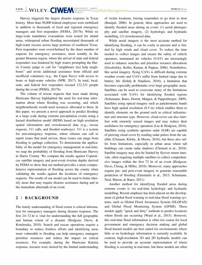
FIGURE 2 Probability of flooding in Harris County during Hurricane Harvey estimated using MaxEnt. Class intervals are created using

standard deviations. The extent of flooding is estimated based on a threshold probability of 0.058

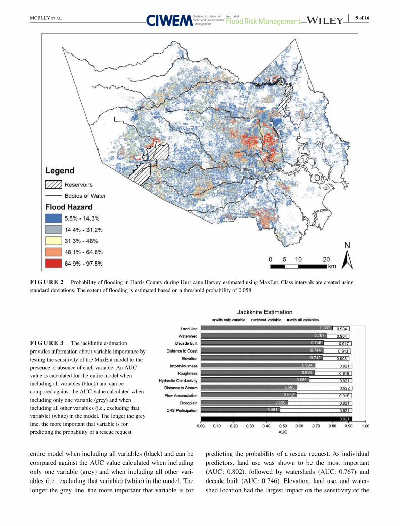
FIGURE 3 The jackknife estimation

provides information about variable importance by

testing the sensitivity of the MaxEnt model to the

presence or absence of each variable. An AUC

value is calculated for the entire model when

including all variables (black) and can be

compared against the AUC value calculated when

including only one variable (grey) and when

including all other variables (i.e., excluding that

variable) (white) in the model. The longer the grey

line, the more important that variable is for

predicting the probability of a rescue request

MOBLEY ET AL. 9 of 16

model; when excluding any one of these three variables, the

AUC dropped to between 0.903 and 0.905. We also find that

two variables negatively influenced the AUC: participation

within the CRS Program and distance to nearest stream fea-

ture. When the model was run without these variables,

model performance increased marginally (AUC: 0.921 and

0.922, respectively). When predicting rescue requests

alone, participation within the CRS Program and location

within the FEMA Special Flood Hazard Area were worse

or close to random predictions (AUC: 0.481 and 0.530,

respectively).

We also analysed the model response curves for each

variable. The response curves indicate how predictive proba-

bilities vary across a single variable when holding all others

constant. We find, for example, locations associated with

residential land use, when compared against all other land

use types, were shown to have the highest probability of

making a rescue request (Figure 4a). We expect that this is

because the majority of rescue requests during Hurricane

Harvey were made at residential properties. Structures built

after 2010 had the highest probability of making a rescue

request, followed by those built in the 1960s and 1970s

(Figure 4b). Locations within the FEMA A-zone, when com-

pared against the V-zone and the areas outside of the 1%

floodplains, had the highest probability of experiencing res-

cue requests (Figure 4c). And, when compared against all

other watersheds, locations in Cypress Creek watershed

(in the northern portion of Harris County) had the highest

probability of making a rescue request (Figure 4d). In addi-

tion, locations associated with lower elevations, as well as

locations closer to streams and farther from the coast had

higher probabilities of making a rescue request.

Finally, based on a lower threshold probability of 0.058,

we estimate that one-third of Harris County (approximately

150,000 Ha) experienced some level of flooding during Hur-

ricane Harvey. The results were visually compared against

the satellite imagery provided by Copernicus and the river-

ine flood extents generated by FEMA (Figure 5). While

Copernicus flood maps did a good job of estimating flooding

in the eastern and western parts of Harris County, they failed

to identify flooding within the urban built environment

where significant numbers of rescue requests were occurring

(e.g., in Greens Bayou, Figure 6). When visually compared

against the modelled extent of flooding predicted by FEMA

as flooded, we find that the HDM predicts a much larger

spatial extent of flooding, indicative of its ability to capture

both out-of-bank riverine flooding along smaller water bod-

ies (e.g., tributaries) and pluvial flooding.

FIGURE 4 Model response curves for the categorical variables (a) land use, (b) decade built, (c) floodplain, and (d) watershed. The response

curves indicate how predictive probabilities vary across a single variable when holding all others constant

10 of 16 MOBLEY ET AL.

FIGURE 5 Copernicus satellite imagery (yellow) and FEMA-estimated riverine flooding (red) shown relative to the maximum flood extent

estimated using MaxEnt (blue)

FIGURE 6 Copernicus satellite imagery

(yellow) and FEMA-estimated riverine flooding

(red) shown relative to the maximum flood extent

estimated using MaxEnt (blue) and the locations of

rescue requests (black) in East Houston

MOBLEY ET AL. 11 of 16

5 | DISCUSSION

The HDM quickly and successfully predicted flood hazard

areas and flood extent within Harris County. Incorporating

VGI data with the MaxEnt software and constraining vari-

ables identified areas that likely needed rescue. Some of the

model results were intuitive, for instance, there were fewer

rescue calls in high elevation areas and residential land uses

were found to have a higher probability of a rescue request

than areas associated with other land uses, such as transpor-

tation infrastructure or parks. Other variables had more sur-

prising influences on the probability of making a rescue

request (i.e., flooding). For instance, participation within the

CRS Program, which has been shown to reduce household

flood damages (Highfield & Brody, 2017) had little bearing

on the flood hazard calculated by MaxEnt. This lack of

influence may be due to a misconfiguration of the variable.

Many communities within Texas participate within the CRS

Program including, for example, the cities of Houston and

Bellaire. Because nearly all communities within Harris

County are participating within the CRS Program, using a

binary variable to represent participation showed so little

variation across the county that it did not explain anything

about the impact of participation. At a larger spatial scale,

we would expect to see a negative correlation between par-

ticipation and flooding. Future research should also explore

other ways to include this variable, such as using CRS score

instead of a binary variable.

Interestingly, structures built in the last decade had the

highest probability of flooding. We would expect that struc-

tures built in the last decade would have the lowest structural

vulnerability due to improvements in building codes and

floodplain regulations over the previous century; however,

we also recognise that making a rescue request does not nec-

essarily suggest that a structure was damaged, but that a

neighbourhood was inundated. For instance, rescue requests

could have occurred due to power outages, lack of food, or

flooded streets, as was also seen in the 311 data set. Even

though the newest homes are typically built to the highest

standards, many of new developments in Harris County have

been built in some of the most flood-prone locations, such as

within Addicks and Barker Reservoirs. Further research

should explore whether the probability of a location flooding

is reflected in damages by comparing the model results

against federal assistance data.

One significant advantage of the HDM over more tradi-

tional flood models is that it is capable of rapidly identifying

flooding in urban areas at a high spatial resolution.

Zooming-in to two neighbourhoods that were especially

hard hit by flooding during Hurricane Harvey, Meyerland

and Friendswood (Figure 7), one can quickly see the added

value of MaxEnt for predicting flooding at the

neighbourhood scale and for allocating emergency resources

in real-time. Here, the estimated extent of flooding from the

HDM was significantly larger than the areas shown as

flooded by FEMA or Copernicus SAR, suggesting that the

HDM provides a more comprehensive map of pluvial

flooding when compared against the preliminary FEMA

flood extents which only consider interpolated riverine flood

depths.

It is important to point out that while the HDM better rep-

resents areas where overland flooding is likely to occur, the

model fails to represent flooded areas with land uses that do

not have rescue calls. For instance, parks and undeveloped

land (including the undeveloped areas behind Addicks and

Barker dams) have much lower probability of a rescue call,

and so the model fails to identify many of these areas as

flooded. This likely has little impact on emergency response

as the areas are not populated but does limit the use of the

model to predict actual flood extent or as a replacement for

high resolution hydraulic modelling, however it is important

to note this limitation when showing this information to the

public, as they may take the maps at face value. The effec-

tiveness of the HDM for identifying flooding in rural areas

where fewer rescue requests may be taking place is currently

unknown. This is because the scope of the study focused on

Harris County, a primarily urban county. Previous studies

suggest that a MaxEnt HDM would be sensitive to rural

flooding (Tehrany et al., 2014). However, the use of VGI

data in a rural landscape has not occurred to date.

6 | CONCLUSION

In this paper, we built an HDM using the MaxEnt software

to demonstrate the applicability of the model for emergency

management in real time, and to predict localised flooding

and total flood extent in Harris County, Texas during Hurri-

cane Harvey. We use several physical and environmental

variables, along with rescue requests to generate a map of

areas in need of emergency services during the event. The

model performed well across three test datasets: a 15% sub-

set of the rescue requests, Houston's 311 flood calls, and

inundated roadways. Most notably, the subset of the rescue

requests and the 311 calls fit excellently (AUC >0.9; Swets,

1988). The model was used to identify flooded urban areas,

many of which were not initially detected using satellite

imagery or estimated riverine floodplains. Runs were per-

formed in less than an hour (wall-clock time) on a personal

computer and successful runs could start with as few as five

requests (Hernandez, Graham, Master, & Albert, 2006), pro-

viding an initial analysis of the extent of flooding and all-

owing emergency managers to prioritise flooded areas

throughout an event. If used in real time, the speed and

12 of 16 MOBLEY ET AL.

accuracy of this model could potentially decrease the time

needed for search and rescue and reduce flood fatalities.

This study was an initial proof of concept for rapid flood

hazard mapping using MaxEnt. However, the current model

build has a few limitations that should be addressed in future

studies. First, while we were able to successfully predict

flooding during a single event, a more robust model account-

ing for multiple historical events would give a better under-

standing of whether MaxEnt can be used to predict flooding

across different types of events. For example, in this model

build, we ignored precipitation as a predictive variable.

Since Hurricane Harvey was the most extreme rain event in

U.S. history and relatively uniform across the study area, we

assumed that this would have little impact on the perfor-

mance of our model. However, during recent smaller storm

events, like the Memorial Day Storm (2015) and Tax Day

Flood (2016), the heaviest precipitation (and thus the dam-

age) was concentrated in the western portion of the County.

To further operationalise the HDM for flood prediction in

real-time, future studies will explore the influence of total

FIGURE 7 Map of rescue

requests shown relative to probability

of flooding estimated using MaxEnt

near (a) Meyerland in brays bayou

watershed and (b) Friendswood in

Clear Creek watershed. These maps

demonstrate the added value of

MaxEnt for predicting flooding and

allocating emergency resources at the

neighbourhood scale

MOBLEY ET AL. 13 of 16

precipitation volume and intensity on model output. Second,

Harvey was an extremely large event necessitating thou-

sands of rescues that were verified by numerous volunteer

organisations. However, during smaller events, crowds-

ourced and validated rescue requests may not be as available

over such a large area. Thus, future studies should also

explore the applicability of MaxEnt using other types of

VGI data available during floods, such as digital images and

hashtags posted by affected populations.

ACKNOWLEDGEMENTS

This work was funded by the NSF PIRE grant no. OISE-

1545837. The authors would like to acknowledge the hospi-

tality and support of the Department of Hydraulic Engineer-

ing at Delft University of Technology during this study.

ORCID

William Mobley https://orcid.org/0000-0003-1783-0599

REFERENCES

Avvenuti, M., Cimino, M. G., Cresci, S., Marchetti, A., & Tesconi, M.

(2016). A framework for detecting unfolding emergencies using

humans as sensors. Springerplus, 5, 43.

Banipal, K. (2006). Strategic approach to disaster management: Les-

sons learned from hurricane Katrina. Disaster Prevention and Man-

agement: An International Journal, 15, 484–494.

Bar Massada, A., Syphard, A. D., Stewart, S. I., & Radeloff, V. C.

(2013). Wildfire ignition-distribution modelling: A comparative

study in the Huron–Manistee National Forest, Michigan, USA.

International Journal of Wildland Fire, 22, 174–183.

Bartoli, G., Fantacci, R., Gei, F., Marabissi, D., & Micciullo, L. (2015).

A novel emergency management platform for smart public safety.

International Journal of Communication Systems, 28, 928–943.

Bean, W. T., Stafford, R., & Brashares, J. S. (2012). The effects of

small sample size and sample bias on threshold selection and accu-

racy assessment of species distribution models. Ecography, 35,

250–258.

Blessing, R., Sebastian, A., & Brody, S. D. (2017). Flood risk delinea-

tion in the U.S.: How much loss are we capturing? Natural Hazards

Review, 18(3), 1–10.

Brody, S. D., Blessing, R., Sebastian, A., & Bedient, P. (2013). Delin-

eating the reality of flood risk and loss in Southeast Texas. Natural

Hazards Review, 14(2), 89–97.

Brody, S. D., Sebastian, A., Blessing, R., & Bedient, P. B. (2018). Case

study results from Southeast Houston, Texas: Identifying the

impacts of residential location on flood risk and loss. Journal of

Flood Risk Management, 11, S110–S120.

Brody, S. D., Zahran, S., Maghelal, P., Grover, H., & Highfield, W. E.

(2007). The rising costs of floods: Examining the impact of plan-

ning and development decisions on property damage in Florida.

Journal of the American Planning Association, 73(3), 330–345.

Clement, M. A., Kilsby, C. G., & Moore, P. (2018). Multi-temporal

synthetic aperture radar flood mapping using change detection.

Journal of Flood Risk Management, 11(2), 152–168.

de Bruijn, J. A., de Moel, H., Jongman, B., Wagemaker, J., &

Aerts, J. C. (2018). TAGGS: Grouping tweets to improve global

geoparsing for disaster response. Journal of Geovisualization and

Spatial Analysis, 2(1), 2.

de Moel, H., & Aerts, J. C. J. H. (2011). Effect of uncertainty in land

use, damage models and inundation depth on flood damage esti-

mates. Natural Hazards, 58(1), 407–425 Available at: http://link.

springer.com/10.1007/s11069-010-9675-6

Eilander, D., Trambauer, P., Wagemaker, J., & Van Loenen, A. (2016).

Harvesting social media for generation of near real-time flood

maps. Procedia Engineering, 154, 176–183.

Elith, J. (2000). Quantitative methods for modeling species habitat:

Comparative performance and an application to Australian plants.

In Quantitative methods for conservation biology. New York, NY:

Springer.

Elith, J., Phillips, S. J., Hastie, T., Dudík, M., Chee, Y. E., &

Yates, C. J. (2011). A statistical explanation of MaxEnt for ecolo-

gists. Diversity and Distributions, 17, 43–57.

Emanuel, K. (2017). Assessing the present and future probability of

Hurricane Harvey's rainfall. Proceedings of the National Academy

of Sciences of the United States of America, 114(48), 12681–

12684.

Engman, E. T. (1986). Roughness coefficients for routing surface run-

off. Journal of Irrigation and Drainage Engineering, 112(1),

39–53.

Erdelj, M., & Natalizio, E. (2016). UAV-assisted disaster management:

Applications and open issues. Paper presented at international con-

ference on computing, networking and communications (ICNC),

IEEE (pp. 1–5).

ESRI. (2017). How Flow Accumulation works [Online]. arcgis.com:

ESRI. Retrieved from http://pro.arcgis.com/en/pro-app/tool-

reference/spatial-analyst/how-flow-accumulation-works.htm.

Faivre, N., Jin, Y., Goulden, M. L., & Randerson, J. T. (2014). Controls

on the spatial pattern of wildfire ignitions in Southern California.

International Journal of Wildland Fire, 23, 799.

FEMA (2017a). Copernicus flood inundation. Retrieved from https://

www.arcgis.com/home/item.html?id=

5b15681cf44645eb858738c831f3ef45#overview.

FEMA (2017b). Historic disaster response to Hurricane Harvey in

Texas. Retrieved from https://www.fema.gov/news-release/2017/

09/22/historic-disaster-response-hurricane-harvey-texas.

FEMA (2017c). Index of /NationalDisasters/HurricaneHarvey/Data/-

DepthGrid/FEMA/ Riverine_Modeled_Preliminary_Observations.

Retrived from https://data.femadata.com/National

Disasters/Hurricane

Harvey/Data/

DepthGrid/FEMA/Riverine_Modeled_Preliminary_Observations/.

Fiedrich, F., Gehbauer, F., & Rickers, U. (2000). Optimized resource

allocation for emergency response after earthquake disasters. Safety

Science, 35, 41–57.

Fohringer, J., Dransch, D., Kreibich, H., & Schröter, K. (2015). Social

media as an information source for rapid flood inundation mapping.

Natural Hazards and Earth System Sciences, 15, 2725–2738.

Gao, H., Barbier, G., & Goolsby, R. (2011). Harnessing the

crowdsourcing power of social media for disaster relief. IEEE Intel-

ligent Systems, 26, 10–14.

14 of 16 MOBLEY ET AL.

Giustarini, L., Hostache, R., Matgen, P., Schumann, G. J. P.,

Bates, P. D., & Mason, D. C. (2013). A change detection approach

to flood mapping in urban areas using TerraSAR-X. IEEE Transac-

tions on Geoscience and Remote Sensing, 51, 2417–2430.

Goodchild, M. F., & Glennon, J. A. (2010). Crowdsourcing geographic

information for disaster response: A research frontier. International

Journal of Digital Earth, 3, 231–241.

Grocholsky, B., Keller, J., Kumar, V., & Pappas, G. (2006). Coopera-

tive air and ground surveillance. IEEE Robotics & Automation

Magazine, 13, 16–25.

Hernandez, P. A., Graham, C. H., Master, L. L., & Albert, D. L.

(2006). The effect of sample size and species characteristics on per-

formance of different species distribution modeling methods.

Ecography, 29, 773–785.

H-GAC. (2017). Census data. Retrieved from: http://www.h-gac.com/

community/socioeconomic/census-data/default.aspx.

Highfield, W. E., & Brody, S. D. (2017). Determining the effects of the

FEMA Community rating system program on flood losses in the

United States. International Journal of Disaster Risk Reduction,

21, 396–404.

Hodgson, M. E., Davis, B. A., Cheng, Y., & Miller, J. (2010). Model-

ing remote sensing satellite collection opportunity likelihood for

hurricane disaster response. Cartography and Geographic Informa-

tion Science, 37(1), 7–15.

Hodgson, M. E., Davis, B. A., & Kotelenska, J. (2010). Remote sensing

and GIS data/information in the emergency response/recovery phase.

In P. S. Showalter & Y. Lu (Eds.), Geospatial techniques in urban

hazard and disaster analysis. Dordrecht, the Netherlands: Springer.

Houston, C. O. (2017). City of Houston 311 help & info [Online]. City

of Houston. Retrieved from: http://www.houstontx.gov/311/.

Hunter, N. M., Bates, P. D., Horritt, M. S., & Wilson, M. D. (2007).

Simple spatially-distributed models for predicting flood inundation:

A review. Geomorphology, 90(3–4), 208–225.

Irza, J. N. (2016). Addressing uncertainty in residential damage esti-

mates from tropical cyclone storm surge with a focus on variability

in structural elevations. Houston, TX: Rice University.

Juan, A., Gori, A., & Sebastian, A. (2017). Comparing floodplain evo-

lution in channelized and un-channelized urban watersheds in

Houston, Texas. Proceedings of conference on World Environmen-

tal and Water Resources Congress.

Kaewkitipong, L., Chen, C., Ractham, P. 2012. Lessons learned from

the use of social media in combating a crisis: A case study of 2011

Thailand flooding disaster. Paper presented at Proceedings of thirty

third international conference on Information Systems,

Orlando, FL.

Kalyanapu, A. J., Burian, S. J., & McPherson, T. N. (2009). Effect of

land use-based surface roughness on hydrologic model output.

Journal of Spatial Hydrology, 9(2), 51–71.

Kennedy, A., Rogers, S., Sallenger, A., Gravois, U., Zachry, B.,

Dosa, M., & Zarama, F. (2011). Building destruction from waves

and surge on the bolivar peninsula during hurricane Ike. Journal of

Waterway, Port, Coastal, and Ocean Engineering, 137(3),

132–14197.

Liu, C., Berry, P. M., Dawson, T. P., & Pearson, R. G. (2005).

Selecting thresholds of occurrence in the prediction of species dis-

tributions. Ecography, 28(3), 385–393.

Liu, S., & Hodgson, M. E. (2016). Satellite image collection modeling

for large area hazard emergency response. ISPRS Journal of Photo-

grammetry and Remote Sensing, 118, 13–21.

Miller, C., & Ager, A. A. (2013). A review of recent advances in risk

analysis for wildfire management. International Journal of Wild-

land Fire, 22(1), 14.

NPR. (2017). Harris county judge calls houston flooding “unprece-

dented.” Retrived from https://www.npr.org/2017/08/28/

546831696/harris-county-judge-calls-houston-flooding-

unprecedented.

Okolloh, O. (2009). Ushahidi, or ‘testimony’: Web 2.0 tools for

crowdsourcing crisis information. Participatory Learning and

Action, 59, 65–70.

Penman, T., Bradstock, R., & Price, O. (2013). Modelling the determi-

nants of ignition in the Sydney Basin, Australia: Implications for

future management. International Journal of Wildland Fire, 22,

469–478.

Phillips, S. J., Anderson, R. P., Dudík, M., Schapire, R. E., &

Blair, M. E. (2017). Opening the black box: An open-source release

of Maxent. Ecography, 40(7), 887–893.

Phillips, S. J., Anderson, R. P., & Schapire, R. E. (2006). Maximum

entropy modeling of species geographic distributions. Ecological

Modelling, 190, 231–259.

Phillips, S. J., & Dudík, M. (2008). Modeling of species distributions

with Maxent: New extensions and a comprehensive evaluation.

Ecography, 31(2), 161–175.

Phillips, S.J., Dudík, M., & Schapire, R. E. (2004). A maximum entropy

approach to species distribution modeling. Paper presented at Pro-

ceedings of the twenty-first international conference on Machine

learning. ACM (p. 83).

Phillips, S.J., Dudík, M., & Schapire, R. E. (2016). Maxent software

for modeling species niches and distributions (Version 3.3).

Retrieved from http://biodiversityinformatics.amnh.org/open_

source/maxent/.

Rahmati, O., Pourghasemi, H. R., & Melesse, A. M. (2016). Applica-

tion of GIS-based data driven random forest and maximum entropy

models for groundwater potential mapping: A case study at Mehran

Region, Iran. Catena, 137, 360–372.

Rawls, W. J., Brakensiek, D. L., & Miller, N. (1983). Green-ampt infil-

tration parameters from soils data. Journal of Hydraulic Engineer-

ing, 109(1), 62–70.

Risser, M. D., & Wehner, M. F. (2017). Attributable human-induced

changes in the likelihood and magnitude of the observed extreme

precipitation during Hurricane Harvey. Geophysical Research Let-

ters, 44, 12,457–12,464.

Sakaki, T., Okazaki, M., & Matsuo, Y. (2013). Tweet analysis for real-

time event detection and earthquake reporting system development.

IEEE Transactions on Knowledge and Data Engineering, 25,

919–931.

Schnebele, E., & Waters, N. (2014). Road assessment after flood events

using non-authoritative data. Natural Hazards and Earth System

Sciences, 14, 1007–1015.

Schumann, G., Bates, P. D., Horritt, M. S., Matgen, P., &

Pappenberger, F. (2009). Progress in integration of remote sensing–

derived flood extent and stage data and hydraulic models. Reviews

of Geophysics, 47(4), RG4001. https://doi.org/10.1029/2008R

G000274.

Schumann, G. J.-P., Neal, J. C., Mason, D. C., & Bates, P. D.

(2011). The accuracy of sequential aerial photography and SAR

data for observing urban flood dynamics, a case study of the

UKsummer 2007 floods. Remote Sensing of Environment, 115,

2536–2546.

MOBLEY ET AL. 15 of 16

Scott, J., Helmbrecht, D., Parks, S., & Miller, C. (2012). Quantifying

the threat of unsuppressed wildfires reaching the adjacent wildland-

urban interface on the Bridger-Teton National Forest, Wyoming,

USA. Fire Ecology, 8, 125–142.

Sebastian, A. (2016). Quantifying flood hazard and risk in highly

urbanized coastal watersheds. Houston, TX: Rice University.

Siahkamari, S., Haghizadeh, A., Zeinivand, H., Tahmasebipour, N., &

Rahmati, O. (2017). Spatial prediction of flood-susceptible areas

using frequency ratio and maximum entropy models. Geocarto

International, 33(9), 927–941.

Sreerama, K., & Varshney, L. (2017). City of Houston Department of

Public Works and Engineering Infrastructure Design Manual,

Houston, TX. Retrieved from https://edocs.publicworks.houstontx.

gov/documents/design_manuals/idm.pdf.

Swets, J. (1988). Measuring the accuracy of diagnostic systems. Sci-

ence, 240, 1285–1293.

Syphard, A. D., & Keeley, J. E. (2015). Location, timing and extent of

wildfire vary by cause of ignition. International Journal of Wild-

land Fire, 24, 37–47.

Tehrany, M. S., Pradhan, B., & Jebur, M. N. (2013). Spatial prediction

of flood susceptible areas using rule based decision tree (DT) and a

novel ensemble bivariate and multivariate statistical models in GIS.

Journal of Hydrology, 504, 69–79.

Tehrany, M. S., Pradhan, B., & Jebur, M. N. (2014). Flood susceptibil-

ity mapping using a novel ensemble weights-of-evidence and

support vector machine models in GIS. Journal of Hydrology, 512,

332–343.

Triglav-Čekada, M., & Radovan, D. (2013). Using volunteered geo-

graphical information to map the November 2012 floods in Slove-

nia. Natural Hazards and Earth System Sciences, 13, 2753–2762.

USDA. (2003). Web soil survey. Retrieved from http://websoilsurvey.

sc.egov.usda.gov/App/WebSoilSurvey.aspx.

van Oldenborgh, G. J., van der Wiel, K., Sebastian, A., Singh, R.,

Arrighi, J., Otto, F., … Cullen, H. (2017). Attribution of extreme

rainfall from Hurricane Harvey. Environmental Research Letters,

12, 124009.

Ward, P. J., Jongman, B., Salamon, P., Simpson, A., Bates, P., De

Groeve, T., … Winsemius, H. C. (2015). Usefulness and limitations

of global flood risk models. Nature Climate Change, 5, 712–715.

How to cite this article: Mobley W, Sebastian A,

Highfield W, Brody SD. Estimating flood extent

during Hurricane Harvey using maximum entropy to

build a hazard distribution model. J Flood Risk

Management. 2019;12 (Suppl. 1):e12549. https://doi.

org/10.1111/jfr3.12549

16 of 16 MOBLEY ET AL.

View publication statsView publication stats