http://www.econometricsociety.org/

Econometrica, Vol. 86, No. 2 (March, 2018), 737–761

ESTIMATING SEMI-PARAMETRIC PANEL MULTINOMIAL CHOICE MODELSUSING CYCLIC MONOTONICITY

XIAOXIA SHIDepartment of Economics, University of Wisconsin-Madison

MATTHEW SHUMDivision of Humanities and Social Sciences, Caltech

WEI SONGGregory and Paula Chow Center for Economic Research (GCCER) and Department of

Statistics, School of Economics, Xiamen University

The copyright to this Article is held by the Econometric Society. It may be downloaded, printed and re-produced only for educational or research purposes, including use in course packs. No downloading orcopying may be done for any commercial purpose without the explicit permission of the Econometric So-ciety. For such commercial purposes contact the Office of the Econometric Society (contact informationmay be found at the website http://www.econometricsociety.org or in the back cover of Econometrica).This statement must be included on all copies of this Article that are made available electronically or inany other format.

Econometrica, Vol. 86, No. 2 (March, 2018), 737–761

ESTIMATING SEMI-PARAMETRIC PANEL MULTINOMIAL CHOICE MODELSUSING CYCLIC MONOTONICITY

XIAOXIA SHIDepartment of Economics, University of Wisconsin-Madison

MATTHEW SHUMDivision of Humanities and Social Sciences, Caltech

WEI SONGGregory and Paula Chow Center for Economic Research (GCCER) and Department of Statistics,

School of Economics, Xiamen University

This paper proposes a new semi-parametric identification and estimation approachto multinomial choice models in a panel data setting with individual fixed effects. Ourapproach is based on cyclic monotonicity, which is a defining convex-analytic feature ofthe random utility framework underlying multinomial choice models. From the cyclicmonotonicity property, we derive identifying inequalities without requiring any shaperestrictions for the distribution of the random utility shocks. These inequalities pointidentify model parameters under straightforward assumptions on the covariates. Wepropose a consistent estimator based on these inequalities.

KEYWORDS: Cyclic monotonicity, multinomial choice, panel data, fixed effects, con-vex analysis.

1. INTRODUCTION

CONSIDER A PANEL MULTINOMIAL CHOICE PROBLEM where agent i chooses from K + 1options (labeled k = 0� � � � �K). Choosing option k in period t gives the agent indirectutility

β′Xkit +Ak

i + εkit� (1.1)

where Xkit is a dx-dimensional vector of observable covariates that has support X , β is

the vector of weights for the covariates in the agent’s utility, Aki is an agent/alternative-

specific fixed effect, and εkit are unobservable utility shocks the distribution of which is notspecified. The agent chooses the option that gives her the highest utility:

Ykit = 1

{β′Xk

it +Aki + εkit ≥ β′Xk′

it +Ak′i + εk

′it ; ∀k′}� (1.2)

where Ykit denotes the multinomial choice indicator. Let the data be identically and in-

dependently distributed (i.i.d.) across i. As is standard in semi-parametric settings, we

Xiaoxia Shi: xshi@ssc.wisc.eduMatthew Shum: mshum@caltech.eduWei Song: wsong@xmu.edu.cnWe thank Khai Chiong, Federico Echenique, Bruce E. Hansen, Whitney Newey, Jack R. Porter, and sem-

inar audiences at Brown, Michigan State, Ohio State, Chicago Booth, Johns Hopkins, Northwestern, NYU,UC Riverside, UNC, Princeton, Cornell, the 2016 Seattle-Vancouver Econometrics Conference, the 2015 Xi-amen/WISE Econometrics Conference in Honor of Takeshi Amemiya, the 2016 Interaction Conference atNorthwestern, the 2016 Conference on Nonstandard Problems at Duke, and the 2017 Cornell-Penn StateIO and Econometrics Conference for useful comments. Alejandro Robinson-Cortes, Pengfei Sui, and JunZhang provided excellent research assistance. Xiaoxia Shi acknowledges the financial support of the Wiscon-sin Alumni Research Foundation via the Graduate School Fall Competition Grant for the year 2014–2015.

© 2018 The Econometric Society https://doi.org/10.3982/ECTA14115

738 X. SHI, M. SHUM, AND W. SONG

normalize ‖β‖ = 1, X0it = 0dx , and A0

i = ε0it = 0. We do not impose any location normal-

ization on εkit or Aki , and as a result, it is without loss of generality to assume that Xk

it doesnot contain a constant.

In this paper, we propose a new semi-parametric approach to the identification and es-timation of β. We exploit the notion of cyclic monotonicity, which is an appropriate gener-alization of “monotonicity” to multivariate (i.e., vector-valued) functions. The notion hasnot been used as a tool for the identification and estimation of semi-parametric multi-nomial choice models, although the cyclic monotonicity between consumption and pricein a representative consumer basket has been used in econometrics as early as Browning(1989) for testing rational expectation hypotheses.

In cross-sectional multinomial models, it is easy to show that there is a cyclic monotonic-ity relationship between the conditional choice probability and the utility index vectorunder independence between the unobservable shocks and the utility indices. We applythat to the panel model given above, find a way to integrate out the fixed effects, and ob-tain a collection of conditional moment inequalities which, conveniently, are linear in β.Then we show that these moment inequalities point identify β under either of two sets ofprimitive verifiable conditions. We finally propose a consistent estimator for β, the com-putation of which requires only convex optimization and thus is not sensitive to startingvalues of the optimization routine.

This paper is most closely related to several contemporaneous papers. Pakes and Porter(2013) proposed a different approach to construct moment inequalities for the panel datamultinomial choice model, based on ranking the options according to their conditionalchoice probabilities. By comparison, we compare the entire vector of choice probabili-ties for all options across time periods. Khan, Ouyang, and Tamer (2016) proposed anapproach to point identification in a dynamic panel setting. Some of their identificationstrategies are similar to ours, but our estimators are rather different.

Our paper builds upon the existing literature on semi-parametric panel binary choicemodels. Manski (1987) proposed the maximum score approach for identification andestimation. Honoré and Kyriazidou (2000) used a maximum score-type estimator for adynamic panel binary choice model. Abrevaya (2000) proposed a general class of rank-correlation estimators, which is a smoothed version of Manski’s (1987) estimator whenapplied to the panel binary choice models. Honoré and Lewbel (2002) generalized thespecial regressor approach of Lewbel (1998, 2000) to the panel data setting.

Semi-parametric identification and estimation of multinomial choice models have beenconsidered in cross-sectional settings (i.e., models without individual fixed effect). Manski(1975) and Fox (2007) based identification on the assumption of a rank-order property thatthe ranking of β′Xk

i across k is the same as that of E[Yki |X1

i � � � � �XKi ] across k; this is an

IIA-like property that allows utility comparisons among all the options in the choice set tobe decomposed into pairwise comparisons among these options. To ensure this rank-orderproperty, Manski assumed that the error terms are i.i.d. across k, while Fox relaxed thei.i.d. assumption to exchangeability. Exchangeability (or the rank-order property) is notused in our approach. Lewbel (2000) considered identification using a special regressor.In addition, Powell and Ruud (2008) and Ahn, Ichimura, Powell, and Ruud (2018) con-sidered an approach based on matching individuals with equal conditional choice proba-bilities, which requires that the rank of a certain matrix formed from the data be deficientby exactly 1. This approach does not obviously extend to the panel data setting with fixedeffects.

The existing literature on cross-sectional binary choice models and on the semi-parametric estimation of single or multiple index models (which include discrete choice

SEMI-PARAMETRIC PANEL MULTINOMIAL CHOICE MODELS 739

models as examples) is voluminous and less relevant for us, and thus is not reviewed herefor brevity.1

The paper proceeds as follows. In Section 2, we introduce the notion of cyclic mono-tonicity and relate it to a generic multinomial choice model. Subsequently, in Section 3,we present the moment inequalities emerging from cyclic monotonicity for panel multino-mial choice models, and give assumptions under which these inequalities suffice to pointidentify the parameters of interest. This section also contains examples where the pointidentification assumptions are verified. Section 4 presents an estimator, shows its consis-tency, and evaluates its performance using Monte Carlo experiments. Sections 3 and 4focus on 2-period panels and length-2 cycles. In Section 5, we extend the discussion tolonger panels and longer cycles. In Section 6, we discuss the closely related aggregatepanel multinomial choice model, which is a workhorse model for demand modeling inempirical industrial organization. This section also contains an illustrative empirical ap-plication using aggregate supermarket scanner data. Section 7 concludes.

2. PRELIMINARIES

In this section, we describe the concept of cyclic monotonicity and its connection tomultinomial choice models. We begin by providing the definition of cyclic monotonicity.

DEFINITION 1—Cyclic Monotonicity: Consider a function f : U → RK where U ⊆ RK ,and a length-M cycle of points in RK : u1�u2� � � � � uM�u1. The function f is cyclic monotonewith respect to the cycle u1�u2� � � � � uM�u1 if 2

M∑m=1

(um − um+1)′f (um)≥ 0� (2.1)

where uM+1 = u1. The function f is cyclic monotone on U if it is cyclic monotone withrespect to all possible cycles of all lengths on its domain.

Cyclic monotonicity is defined for mappings from RK → RK , which generalizes theusual monotonicity for real-valued functions. We make use of the following basic resultwhich relates cyclic monotonicity to convex functions:

PROPOSITION 1—Cyclic Monotonicity and Convexity: Consider a differentiable functionF : U → R for an open convex set U ⊆ RK . If F is convex on U , then the gradient of F(denoted ∇F(u) := ∂F(u)/∂u) is cyclic monotone on U .

The proof for Proposition 1 is available from standard sources (e.g., Rockafellar (1970,Chapter 24), Villani (2003, Section 2.3)). Consider a univariate and differentiable con-vex function; obviously, its slope must be monotonically nondecreasing. The above resultstates that cyclic monotonicity is the appropriate extension of this feature to multivariateconvex functions.

Now we connect the above discussion to the multinomial choice model. We start witha generic random utility model for multinomial choices without specifying the random

1An exhaustive survey is provided in Horowitz (2009), Chapters 2 and 3.2Technically, this defines the property of being “cyclic monotonically increasing,” but for notational simplic-

ity and without loss of generality, we use “cyclic monotone” for “cyclic monotonically increasing.”

740 X. SHI, M. SHUM, AND W. SONG

utility function or the data structure in detail. Suppose that an agent is choosing fromK+1 choices 0�1� � � � �K. The utility that she derives from choice k is partitioned into twoadditive parts: Uk + εk, where Uk denotes the systematic component of the latent utility,while εk denotes the random shocks, idiosyncratic across agents and choice occasions. Shechooses choice k∗ if Uk∗ + εk

∗ ≥ maxk=0�����K Uk + εk. Let Yk = 1 if she chooses choice k

and 0 otherwise. As is standard, we normalize U0 = ε0 = 0.Let uk denote a generic realization of Uk. Also let U = (U1� � � � �UK)′, u = (u1� � � � � uK)′,

and ε = (ε1� � � � � εK)′. We introduce the “social surplus function” (McFadden (1978,1981)), which is the expected utility obtained from the choice problem:

W(u)=E{

maxk=0�����K

[Uk + εk

]∣∣U = u}� (2.2)

The following lemma shows that this function is convex and differentiable, that its gradi-ent corresponds to the choice probability function, and finally that the choice probabilityfunction is cyclic monotone. The first three parts of the lemma are already known in theliterature (e.g., McFadden (1981)), and the last part is immediately implied by the previ-ous parts and Proposition 1. Nonetheless, we give a self-contained proof in Appendix Afor easy reference for the reader.

LEMMA 2.1—Gradient: Suppose that U is independent of ε and that the distribution of εis absolutely continuous with respect to the Lebesgue measure. Then

(a) W(·) is convex on RK ,(b) W(·) is differentiable on RK ,(c) p(u) = ∇W(u), where p(u)= E[Y|U = u] and Y = (Y 1� � � � �YK)′, and(d) p(u) is cyclic monotone on RK .

The cyclic monotonicity of the choice probability can be used to form identifying re-strictions for the structural parameters in a variety of settings. In this paper, we focus onthe linear panel data model with fixed effects, composed of equations (1.1) and (1.2).

3. PANEL DATA MULTINOMIAL CHOICE MODELS WITH FIXED EFFECTS

We focus on a short panel data setting where there are only two time periods. An exten-sion to multiple time periods is given in Section 5. Let U, ε, and Y be indexed by both i (in-dividual) and t (time period). Thus they are now Uit ≡ (U1

it � � � � �UKit )

′, εit ≡ (ε1it � � � � � ε

Kit )

′,and Yit ≡ (Y 1

it � � � � �YKit )

′. Let there be an observable dx-dimensional covariate Xkit for each

choice k, and let Ukit be a linear index of Xk

it plus an unobservable individual effect Aki :

Ukit = β′Xk

it +Aki � (3.1)

where β is a dx-dimensional unknown parameter. Let Xit = (X1it � � � � �X

Kit ) and Ai =

(A1i � � � � �A

Ki )

′. Note that Xit is a dx × K matrix. In short panels, the challenge in thismodel is the identification of β while allowing correlation between the covariates andthe individual effects. We tackle this problem using the cyclic monotonicity of the choiceprobability, as we explain next.

3.1. Identifying Inequalities

We derive our identification inequalities under the following assumption.

SEMI-PARAMETRIC PANEL MULTINOMIAL CHOICE MODELS 741

ASSUMPTION 3.1: (a) εi1 and εi2 are identically distributed conditional on Ai�Xi1�Xi2:

(εi1 ∼ εi2)|(Ai�Xi1�Xi2)�

(b) the conditional distribution of εit given Ai�Xi1�Xi2 is absolutely continuous with respectto the Lebesgue measure for t = 1�2 everywhere on the support of Ai�Xi1�Xi2.

REMARK: (i) Part (a) of the assumption is the multinomial version of the group homo-geneity assumption of Manski (1987), and is also imposed in Pakes and Porter (2013). Itallows us to form identification inequalities based on the comparison of choices made bythe same individual over different time periods, and by doing this to eliminate the fixedeffect. This assumption rules out dynamic panel models where Xk

it may include lagged val-ues of (Yk

it )Kk=1. But it allows εit to be correlated with the covariates, and allows arbitrary

dependence between εit and the fixed effects.(ii) The assumption imposes no restriction on the dependence amongst the errors. The

errors across choices in a given period can be arbitrarily dependent, and the errors acrosstime periods, although assumed to have identical marginal distributions, can have arbi-trary dependence.

To begin, we let η denote a K-dimensional vector with the kth element being ηk, anddefine

p(η�x1�x2�a)(3.2)

:= (Pr

[εki1 +ηk ≥ εk

′i1 +ηk′ ∀k′|Xi1 = x1�Xi2 = x2�Ai = a

])k=1�����K

�

Assumption 3.1(a) implies that

p(η�x1�x2�a)(3.3)

= (Pr

[εki2 +ηk ≥ εk

′i2 +ηk′ ∀k′|Xi1 = x1�Xi2 = x2�Ai = a

])k=1�����K

�

Assumption 3.1(b) implies that p(η�x1�x2�a) is cyclic monotone in η for all possible val-ues of x1�x2�a. Using the cyclic monotonicity with respect to length-2 cycles, we obtain,for any η1�η2 and x1�x2�a:

(η1 − η2)′[p(η1�x1�x2�a)− p(η2�x1�x2�a)

] ≥ 0� (3.4)

Now we let η1 = X′i1β+ Ai and η2 = X′

i2β+ Ai. Note that for t = 1�2, by the definition ofp(η�x1�x2�a), we have

p(X′

itβ+ Ai�Xi1�Xi2�Ai

) =E[Yit |Xi1�Xi2�Ai]� (3.5)

Combining (3.4) and (3.5), we have(E

[Y′

i1|Xi1�Xi2�Ai

] −E[Y′

i2|Xi1�Xi2�Ai

])(X′

i1β− X′i2β

) ≥ 0 everywhere� (3.6)

Note that the fixed effect differences out within the second parenthetical term on the lefthand-side. Take the conditional expectation given Xi1�Xi2 of both sides, and we get(

E[Y′

i1|Xi1�Xi2

] −E[Y′

i2|Xi1�Xi2

])(X′

i1β− X′i2β

) ≥ 0 everywhere� (3.7)

742 X. SHI, M. SHUM, AND W. SONG

These inequality restrictions involve only identified/observed quantities and the unknownparameter β, and thus can be used to set identify β in the absence of further assumptions,and to point identify β with additional assumptions as discussed below. Note that underbinary choice (K = 1), both terms on the LHS of (3.7) become scalars, so that theseinequalities reduce to the rank correlation result in Manski (1987, Lemma 1).

Hence the foregoing derivations have proved the following lemma:

LEMMA 3.1: Under Assumption 3.1,(E

[Y′

i1|Xi1�Xi2

] −E[Y′

i2|Xi1�Xi2

])(X′

i1β− X′i2β

) ≥ 0 everywhere�

The extension in Section 5 discusses how longer cycles can be used when more timeperiods are available in the data set. The next subsection presents conditions under whichlength-2 cycles are enough to produce point identification.

3.2. Point Identification of Model Parameters

To study the identification information contained in the inequalities in (3.7), we rewritethem as

E[�Y′

i|Xi1�Xi2

]�X′

iβ≥ 0� (3.8)

where �Zi = Zi2 −Zi1.Define g ≡ (�XiE[�Yi|Xi1�Xi2]). For identification, we will want to place restrictions

on the support of the vector g, which we define as

G = supp(g) = supp(�XiE[�Yi|Xi1�Xi2]

)� (3.9)

We would like to find conditions on model primitives (Xit , Ait , and εit) that guaranteethat the support of the vectors g is rich enough to ensure point identification.

First, we impose regularity conditions on the unobservables:

ASSUMPTION 3.2: (a) The conditional support of (εit |Ai�Xi1�Xi2) is RK with positive prob-ability.

(b) The conditional distribution of (εit + Ai) given (Xi1�Xi2) = (x1�x2) is uniformly con-tinuous in (x1�x2). That is,

lim(x1�x2)→(x0

1�x02)

supe�a∈RK

∣∣Fεit+Ai|Xi1�Xi2(e + a|x1�x2)− Fεit+Ai|Xi1�Xi2

(e + a|x0

1�x02

)∣∣ = 0�

The role of Assumption 3.2(a) becomes clear when we describe the covariate condi-tions below. Assumption 3.2(b) is a sufficient condition for the continuity of the func-tion E[�Yi|Xi1 = x1�Xi2 = x2]. The latter ensures that the violation of the inequalityE[�Y′

i|Xi1 = x1�Xi2 = x2]�x′b ≥ 0 for a point (x1�x2) on the support of (Xi1�Xi2) impliesthat the inequality E[�Y′

i|Xi1�Xi2]�X′ib ≥ 0 is violated with positive probability.

We also need a condition on the observable �Xi. In general, this is not straightforward.Note that the vectors g are equal to

�XiE[�Yi|Xi1�Xi2] =K∑

k=1

�Xki E

[�Yk

i |Xi1�Xi2

]� (3.10)

SEMI-PARAMETRIC PANEL MULTINOMIAL CHOICE MODELS 743

In general, it is difficult to formulate conditions on the RHS of the previous equationbecause the RHS is a weighted sum of �Xk

i where the weight is the conditional choiceprobability, which is not a primitive quantity. We proceed by considering two approachesto reduce the RHS to a single term.

There are two types of events conditional on which we can reduce the summation to asingle term:

1. For a given k, let �X−ki = (�X1

i � � � � ��Xk−1i ��Xk+1

i � � � � ��XKi ). Conditional on the

event �X−ki = 0 (i.e., individual i’s covariates are constant across both periods, for all

choices except the kth choice), we have

�XiE[�Yi|Xi1�Xi2] = �Xki E

[�Yk

i |Xi1�Xi2

]�

Note that supp(�Xki E[�Yk

i |Xi1�Xi2]) = supp(�Xki sign(E[�Yk

i |Xi1�Xi2])) due to the factthat E[�Yk

i |Xi1�Xi2] is a scalar random variable. Assumption 3.2(a) ensures that wehave Pr(E[�Yk

i |Xi1�Xi2] = 0|�X−ki = 0) = 0, which implies that sign(E[�Yk

i |Xi1�Xi2]) ∈{−1�1} with probability 1 conditional on �X−k

i = 0. Thus, it is sufficient to assume a richsupport for �Xk

i and −�Xki conditional on �X−k

i = 0. We are thus motivated to define

GI ≡⋃k

supp(±�Xk

i |�X−ki = 0

)� (3.11)

where the conditional support of ±�Xki is the union of the conditional support of �Xk

i

and that of −�Xki .

2. Conditional on the event �Xki = �X1

i for all k (i.e., individual i’s covariates areidentical across all choices and only vary across time periods), we have

�XiE[�Yi|Xi1�Xi2] = �X1i E

[−�Y 0i |Xi1�Xi2

]�

where �Y 0i = −∑K

k=1 �Yki . Similar arguments as above show that it is sufficient to assume

a rich support for �X1i and −�X1

i , which motivates us to define

GII ≡ supp(±�X1

i |�Xki = �X1

i ∀k)� (3.12)

In what follows, our identification condition will be imposed on the set

G≡GI ∪GII� (3.13)

Two assumptions on G are considered, which differ in the types of covariates that theyaccommodate. Each assumption is sufficient by itself. We consider each case in turn.

ASSUMPTION 3.3: The set G contains an open Rdx ball around the origin.

The gist of this assumption is that, beginning from the origin and moving in any direc-tion, we will reach a point in G. This assumption essentially requires all covariates to becontinuous, but allows them to be bounded.

Our second sufficient condition allows discrete covariates generally, but requires oneregressor with large support. Let g−1 denote g with the first element removed, and defineG−1 = {g−1 : ∃g1 ∈ R s.t. (g1� g

′−1)

′ ∈ G}. Let G1(g−1) = {g1 ∈ R : (g1� g′−1)

′ ∈ G}. For j =2� � � � � dx, we define g−j , G−j , and Gj(g−j) analogously.

ASSUMPTION 3.4: For some j∗ ∈ {1�2� � � � � dx}:

744 X. SHI, M. SHUM, AND W. SONG

(a) Gj∗(g−j∗)=R for all g−j∗ in a subset G0−j∗ of G−j∗ ,

(b) G0−j∗ is not contained in a proper linear subspace of Rdx−1,

(c) the j∗th element of β, denoted by βj∗ , is nonzero.

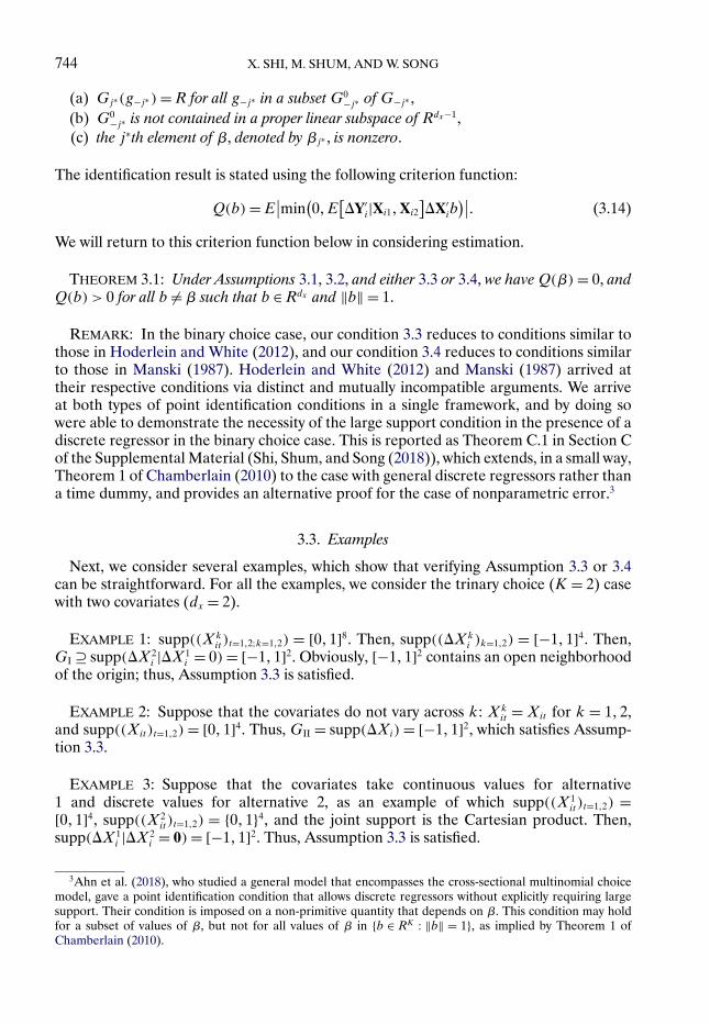
The identification result is stated using the following criterion function:

Q(b) = E∣∣min

(0�E

[�Y′

i|Xi1�Xi2

]�X′

ib)∣∣� (3.14)

We will return to this criterion function below in considering estimation.

THEOREM 3.1: Under Assumptions 3.1, 3.2, and either 3.3 or 3.4, we have Q(β) = 0, andQ(b) > 0 for all b �= β such that b ∈ Rdx and ‖b‖ = 1.

REMARK: In the binary choice case, our condition 3.3 reduces to conditions similar tothose in Hoderlein and White (2012), and our condition 3.4 reduces to conditions similarto those in Manski (1987). Hoderlein and White (2012) and Manski (1987) arrived attheir respective conditions via distinct and mutually incompatible arguments. We arriveat both types of point identification conditions in a single framework, and by doing sowere able to demonstrate the necessity of the large support condition in the presence of adiscrete regressor in the binary choice case. This is reported as Theorem C.1 in Section Cof the Supplemental Material (Shi, Shum, and Song (2018)), which extends, in a small way,Theorem 1 of Chamberlain (2010) to the case with general discrete regressors rather thana time dummy, and provides an alternative proof for the case of nonparametric error.3

3.3. Examples

Next, we consider several examples, which show that verifying Assumption 3.3 or 3.4can be straightforward. For all the examples, we consider the trinary choice (K = 2) casewith two covariates (dx = 2).

EXAMPLE 1: supp((Xkit)t=1�2;k=1�2) = [0�1]8. Then, supp((�Xk

i )k=1�2) = [−1�1]4. Then,GI ⊇ supp(�X2

i |�X1i = 0)= [−1�1]2. Obviously, [−1�1]2 contains an open neighborhood

of the origin; thus, Assumption 3.3 is satisfied.

EXAMPLE 2: Suppose that the covariates do not vary across k: Xkit = Xit for k = 1�2,

and supp((Xit)t=1�2) = [0�1]4. Thus, GII = supp(�Xi) = [−1�1]2, which satisfies Assump-tion 3.3.

EXAMPLE 3: Suppose that the covariates take continuous values for alternative1 and discrete values for alternative 2, as an example of which supp((X1

it)t=1�2) =[0�1]4, supp((X2

it)t=1�2) = {0�1}4, and the joint support is the Cartesian product. Then,supp(�X1

i |�X2i = 0)= [−1�1]2. Thus, Assumption 3.3 is satisfied.

3Ahn et al. (2018), who studied a general model that encompasses the cross-sectional multinomial choicemodel, gave a point identification condition that allows discrete regressors without explicitly requiring largesupport. Their condition is imposed on a non-primitive quantity that depends on β. This condition may holdfor a subset of values of β, but not for all values of β in {b ∈ RK : ‖b‖ = 1}, as implied by Theorem 1 ofChamberlain (2010).

SEMI-PARAMETRIC PANEL MULTINOMIAL CHOICE MODELS 745

EXAMPLE 4: Suppose that the first covariate is a time dummy: Xk1�it = t for all k� t, and

the second covariate has unbounded support: supp((Xk2�it)t=1�2;k=1�2) = (c�∞)4 for some

c ∈ R. Then,

supp(�X1

i |�X1i = �X2

i

) = {1} ×R�

Hence, G ⊇ GII = {−1�1} × R. Let j∗ = 2 (for j∗ as defined in Assumption 3.4), and letG0

−2 = {−1�1}. Assumption 3.4(b) obviously holds. Assumption 3.4(a) also holds becauseG2(−1)= G2(1)=R. Assumption 3.4(c) holds as long as β2 �= 0.

3.4. Remarks: Cross-Sectional Model

In this paper, we have focused on identification and estimation of panel multinomialchoice models. Here we briefly remark on the use of the cyclic monotonicity (CM) in-equalities for estimation in cross-sectional multinomial choice models, which is naturaland can be compared to the large number of existing estimators for these models. Inthe cross-sectional model, the individual-specific effects disappear, leading to the choicemodel

Yki = 1

{β′Xk

i + εki ≥ β′Xk′i + εk

′i for all k′ = 0� � � � �K

}�

Hence, to apply the CM inequalities, the only dimension upon which we can differenceis across individuals. Under the assumptions that the vector of utility shocks εi is (i) i.i.d.across individuals and (ii) independent of the covariates X, the 2-cycle CM inequalityyields that, for all pairs (i� j),(

E[Yi|Xi] −E[Yj|Xj])′(Xi − Xj)

′β ≥ 0�

In particular, for the binary choice case (k ∈ {0�1}), this reduces to(E

[Y 1

i |Xi

] −E[Y 1

j |Xj

])(Xi − Xj)

′β ≥ 0�

which is the estimating equation underlying the maximum score (Manski (1975)) andmaximum rank correlation (Han (1987)) estimators for the binary choice model.

4. ESTIMATION AND CONSISTENCY

In this section, we propose a computationally easy consistent estimator for β, basedon Theorem 3.1. The consistency is obtained when n → ∞ with T fixed. In particu-lar, we focus on T = 2 and only discuss longer panels in Section 5 below. Based onthe panel data set, suppose that there is a uniformly consistent estimator pt(x1�x2) forE(Yit |Xi1 = x1�Xi2 = x2) for t = 1�2. Then we can estimate the model parameters using asample version of the criterion function given in equation (3.14). Specifically, we obtain aconsistent estimator of β as β = β/‖β‖, where

β = arg minb∈Rdx :maxj=1�����dx |bj |=1

Qn(b) and (4.1)

Qn(b) = n−1n∑

i=1

[(b′�Xi

)(�p(Xi1�Xi2)

)]−� (4.2)

746 X. SHI, M. SHUM, AND W. SONG

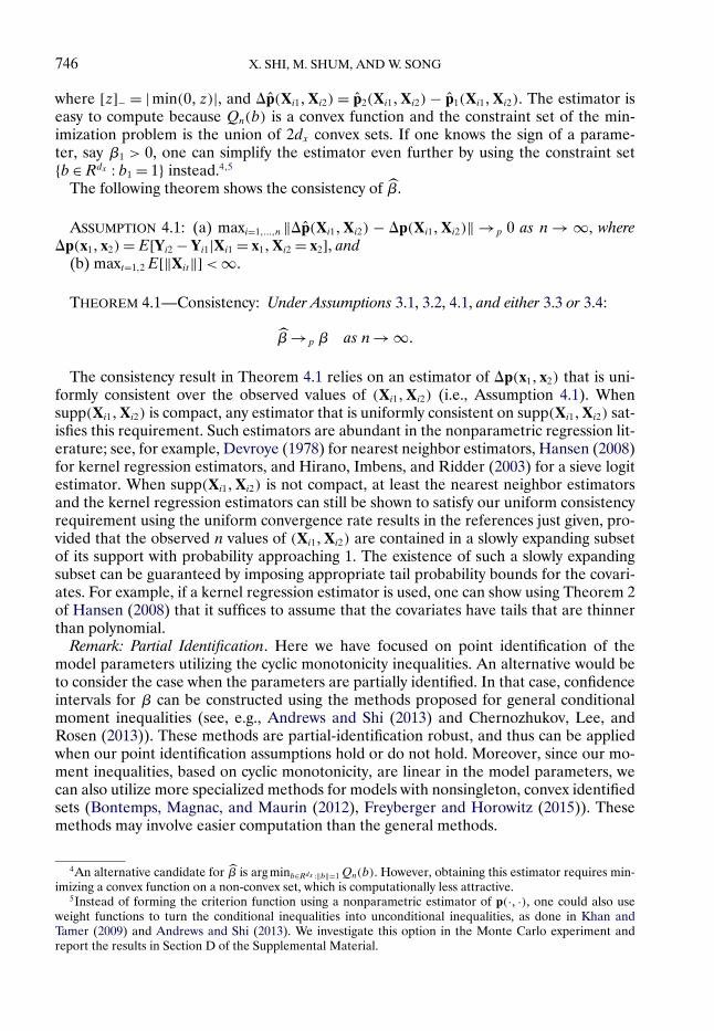
where [z]− = |min(0� z)|, and �p(Xi1�Xi2) = p2(Xi1�Xi2) − p1(Xi1�Xi2). The estimator iseasy to compute because Qn(b) is a convex function and the constraint set of the min-imization problem is the union of 2dx convex sets. If one knows the sign of a parame-ter, say β1 > 0, one can simplify the estimator even further by using the constraint set{b ∈Rdx : b1 = 1} instead.4,5

The following theorem shows the consistency of β.

ASSUMPTION 4.1: (a) maxi=1�����n ‖�p(Xi1�Xi2) − �p(Xi1�Xi2)‖ →p 0 as n → ∞, where�p(x1�x2)= E[Yi2 − Yi1|Xi1 = x1�Xi2 = x2], and

(b) maxt=1�2 E[‖Xit‖] <∞.

THEOREM 4.1—Consistency: Under Assumptions 3.1, 3.2, 4.1, and either 3.3 or 3.4:

β→p β as n → ∞�

The consistency result in Theorem 4.1 relies on an estimator of �p(x1�x2) that is uni-formly consistent over the observed values of (Xi1�Xi2) (i.e., Assumption 4.1). Whensupp(Xi1�Xi2) is compact, any estimator that is uniformly consistent on supp(Xi1�Xi2) sat-isfies this requirement. Such estimators are abundant in the nonparametric regression lit-erature; see, for example, Devroye (1978) for nearest neighbor estimators, Hansen (2008)for kernel regression estimators, and Hirano, Imbens, and Ridder (2003) for a sieve logitestimator. When supp(Xi1�Xi2) is not compact, at least the nearest neighbor estimatorsand the kernel regression estimators can still be shown to satisfy our uniform consistencyrequirement using the uniform convergence rate results in the references just given, pro-vided that the observed n values of (Xi1�Xi2) are contained in a slowly expanding subsetof its support with probability approaching 1. The existence of such a slowly expandingsubset can be guaranteed by imposing appropriate tail probability bounds for the covari-ates. For example, if a kernel regression estimator is used, one can show using Theorem 2of Hansen (2008) that it suffices to assume that the covariates have tails that are thinnerthan polynomial.

Remark: Partial Identification. Here we have focused on point identification of themodel parameters utilizing the cyclic monotonicity inequalities. An alternative would beto consider the case when the parameters are partially identified. In that case, confidenceintervals for β can be constructed using the methods proposed for general conditionalmoment inequalities (see, e.g., Andrews and Shi (2013) and Chernozhukov, Lee, andRosen (2013)). These methods are partial-identification robust, and thus can be appliedwhen our point identification assumptions hold or do not hold. Moreover, since our mo-ment inequalities, based on cyclic monotonicity, are linear in the model parameters, wecan also utilize more specialized methods for models with nonsingleton, convex identifiedsets (Bontemps, Magnac, and Maurin (2012), Freyberger and Horowitz (2015)). Thesemethods may involve easier computation than the general methods.

4An alternative candidate for β is arg minb∈Rdx :‖b‖=1 Qn(b). However, obtaining this estimator requires min-imizing a convex function on a non-convex set, which is computationally less attractive.

5Instead of forming the criterion function using a nonparametric estimator of p(·� ·), one could also useweight functions to turn the conditional inequalities into unconditional inequalities, as done in Khan andTamer (2009) and Andrews and Shi (2013). We investigate this option in the Monte Carlo experiment andreport the results in Section D of the Supplemental Material.

SEMI-PARAMETRIC PANEL MULTINOMIAL CHOICE MODELS 747

4.1. Monte Carlo Simulation

Consider a trinary choice example and a 2-period panel. Let Xkit be a three-dimensional

covariate vector: Xkit = (Xk

j�it)j=1�2�3. Let (Xkj�it)j=1�2�3;k=1�2;t=1�2 be independent uniform ran-

dom variables in [0�1].6 Let Aki = (ωk

i +X1�i2 −X1�i1)/4 for k= 1�2, where ωki is uniform

in [0�1], independent across k and independent of other model primitives. Consider thetrue parameter value β = (1�0�5�0�5), and use the scale normalization β1 = 1.

We consider two specifications. The first specification is a multinomial logit model. Inthe second specification, εkit for k = 1�2 is a difference of two independent Cauchy(x0 =0�γ = 2) variates.

In addition to our CM estimator, we also implement Chamberlain’s (1980) conditionallikelihood estimator for comparison.7 The conditional likelihood method is consistentand n−1/2-normal for the logit specification, but it may not be consistent in the Cauchyspecification. For both estimators, we report bias, standard deviation (SD), and the rootmean-squared error (rMSE). To implement our estimator, we use the Nadaraya–Watsonestimator with product kernel to estimate p(·� ·) with bandwidth selected via leave-one-out cross-validation. We consider four sample sizes 250, 500, 1000, and 2000, and use 5000Monte Carlo repetitions.

The results are reported in Tables I and II. We only report the performance of β2 be-cause that of β3 is nearly the same due to the symmetric design of the experiment. Un-der the Logit design (Table I), the conditional likelihood estimator not surprisingly hassmaller bias and smaller standard deviation. Yet our CM estimator is close in perfor-mance with conditional likelihood. Under the Cauchy design, the conditional likelihoodestimator displays larger bias and standard deviation, and the bias shrinks very slowly withthe sample size. This may reflect the inconsistency of the conditional likelihood estimatorin this setup. On the other hand, the CM estimator has a smaller bias and standard devia-tion, both decreasing significantly as the sample size increases. Overall, our CM estimatorhas more robust performance in non-logit setup and leads to only modest efficiency lossin the logit setups in the range of sample sizes that we consider.8

5. LONGER PANELS (T > 2)

We have thus far focused on 2-period panel data sets for ease of exposition. Our methodnaturally generalizes to longer panel data sets as well. Suppose that there are T timeperiods. Then one can use all cycles with length L ≤ T to form the moment inequalities.To begin, consider t1� t2� � � � � tL ∈ {1�2� � � � �T }, where the points do not need to be alldistinct. Assuming the multi-period analogue of Assumption 3.1, we can use derivation

6Assumption 3.3 is satisfied because all the X variables are supported on the unit interval and they can varyfreely from each other. Thus point identification holds under this design.

7In Section C of the Supplemental Material, we report an instrumental function variation of our estimator,where the conditional moment inequalities are approximated by unconditional moment inequalities generatedby multiplying the moment function to indicators of hypercubes on the space of the conditioning variables inthe spirit of Khan and Tamer (2009) and Andrews and Shi (2013), instead of estimated nonparametrically. Thisvariation of our estimator is more difficult to compute and has less desirable Monte Carlo performance.

8As the sample size gets larger, the discrepancy between the standard deviation of the CM estimator andthe conditional likelihood estimator may grow because the latter is n−1/2-consistent while the former likelyconverges more slowly.

748 X. SHI, M. SHUM, AND W. SONG

TABLE I

MONTE CARLO PERFORMANCE OF ESTIMATORS OF β2 (LOGIT DESIGN, β0�2 = 0�5)

n BIAS SD rMSE 25% Quantile Median 75% Quantile

CM Estimator250 −0�0622 0.1385 0.1519 0.3435 0.4302 0.5242500 −0�0484 0.0977 0.1090 0.3854 0.4477 0.5141

1000 −0�0328 0.0701 0.0774 0.4192 0.4647 0.51332000 −0�0257 0.0488 0.0552 0.4402 0.4726 0.5069

Conditional Likelihood Estimator250 0�0064 0.1283 0.1284 0.4192 0.4992 0.5862500 0�0022 0.0888 0.0889 0.4419 0.5009 0.5581

1000 0�0016 0.0621 0.0621 0.4592 0.5004 0.54302000 −0�0001 0.0439 0.0439 0.4700 0.4994 0.5287

similar to that in Section 3.1 to obtain

L∑m=1

β′(Xitm − Xitm+1)E[Yitm |Xit1� � � � �XitL] ≥ 0� (5.1)

To form an estimator, we consider an estimator ptm(Xit1� � � � �XitL) of E[Yitm |Xit1� � � � �XitL].Let the sample criterion function be

Qn(b) = n−1n∑

i=1

∑t1�����tL∈{1�����T }

[L∑

m=1

b′(Xitm − Xitm+1)ptm(Xit1� � � � �XitL)

]−� (5.2)

The estimator of β, β is defined based on Qn(b) in the same way as in Section 4.If L = T , the estimator just defined utilizes all available inequalities implied by cyclic

monotonicity. However, in practice there are disadvantages of using long cycles because(1) the estimator ptm(Xit1� � � � �XitL) can be noisy when t1� � � � � tL contains many distinctvalues, and (2) it is computationally more demanding to exhaust and aggregate all cyclesof longer length if T is moderately large. Thus, in the empirical application below, we onlyuse the length-2 cycles, that is, L = 2.

TABLE II

MONTE CARLO PERFORMANCE OF ESTIMATORS OF β2 (CAUCHY DESIGN, β0�2 = 0�5)

n BIAS SD rMSE 25% Quantile Median 75% Quantile

CM Estimator250 −0�1164 0.2156 0.2450 0.2393 0.3761 0.5226500 −0�0698 0.1714 0.1851 0.3124 0.4237 0.5379

1000 −0�0392 0.1291 0.1349 0.3701 0.4587 0.54542000 −0�0151 0.0953 0.0965 0.4209 0.4809 0.5462

Conditional Likelihood Estimator250 0�1791 0.5985 0.6247 0.4118 0.6014 0.8467500 0�1304 0.2512 0.2830 0.4613 0.6018 0.7607

1000 0�1166 0.1642 0.2013 0.5038 0.6045 0.71822000 0�1110 0.1142 0.1593 0.5327 0.6042 0.6809

SEMI-PARAMETRIC PANEL MULTINOMIAL CHOICE MODELS 749

TABLE III

MOMENT INEQUALITY ESTIMATOR OF β2 (T = 3, CAUCHY DESIGN, β0�2 = 0�5)

n BIAS SD rMSE 25% Quantile Median 75% Quantile

Based on Length-2 Cycles Only250 −0�1413 0.1393 0.1984 0.2631 0.3565 0.4506500 −0�0989 0.1069 0.1457 0.3283 0.3997 0.4716

1000 −0�0693 0.0814 0.1069 0.3755 0.4300 0.48372000 −0�0467 0.0616 0.0773 0.4120 0.4529 0.4936

Based on All Cycles250 −0�1436 0.1391 0.1999 0.2613 0.3553 0.4465500 −0�1006 0.1069 0.1467 0.3254 0.3973 0.4683

1000 −0�0702 0.0817 0.1077 0.3736 0.4291 0.48372000 −0�0478 0.0618 0.0782 0.4108 0.4514 0.4920

For identification, it might be possible to obtain weaker conditions for point identifi-cation when longer cycles are used, but we were not able to come up with a clean set ofconditions for that. For estimation, inequalities from longer cycles provide additional re-striction on the parameter and thus could potentially improve efficiency. We investigatethe gain in a Monte Carlo experiment next.

Another interesting question is whether equation (5.1) with L = T exhausts all theinformation in the random utility model and leads to the sharp identified set. We believethis is unlikely in general because the CM inequalities only derive from the convexity ofthe social surplus function, and do not use other properties of the random utility model.For instance, in random utility models, the choice probability of one alternative shouldnot increase when its own utility index stays constant while the utility indices of the otheralternatives weakly increase, which is not captured in the CM inequalities.9 However,these properties are not straightforward to use in the panel data setting and do not leadto simple linear (in parameters) moment conditions.

5.1. Monte Carlo Results Using Longer Cycles

Here we use a 3-period extension of the Cauchy design presented in the previous sec-tion. All the specification details are the same (including the fact that Ak

i depends onlyon Xk

1�i2 − Xk1�i1), except that one additional period of data is generated. In Table III, we

report the performance of our moment inequality estimators for β2 using length-2 cycles,and using both length-2 and -3 cycles (all cycles). As we can see, the performance of theestimator is nearly identical whether or not the length-3 cycles are used. In practice, onecan try using length-2 cycles only first and then add length-3 cycles to see if the resultschange. If not, there should be no reason to consider longer cycles since longer cyclesinvolve higher computational cost.

6. RELATED MODEL: AGGREGATE PANEL MULTINOMIAL CHOICE MODEL

Up to this point, we have focused on the setting when the researcher has individual-level panel data on multinomial choice. In this section, we discuss an important and sim-pler related model: the panel multinomial choice model estimated using aggregate data

9These other properties were studied in Koning and Ridder (2003).

750 X. SHI, M. SHUM, AND W. SONG

for which we are able to derive some inference results. Such models are often encoun-tered in empirical industrial organization.10 In this setting, the researcher observes theaggregated choice probabilities (or market shares) for the consumer population in a num-ber of regions and across a number of time periods. Correspondingly, the covariates arealso only observed at region/time level for each choice option. To be precise, we observe(Sct�Xct = (X1�′

ct � � � � �XK�′ct )′)n�Tc=1�t=1 which denote, respectively, the region/time-level choice

probabilities and covariates. Only a “short” panel is required, as our approach works withas few as two periods. Thus, to get the idea across with the simplest notation possible, wefocus on the case where T = 2.

We model the individual choice Yict = (Y 1ict � � � � �Y

Kict)

′ as

Ykict = 1

{β′Xk

ct +Akic + εkict ≥ β′Xk′

ct +Ak′ic + εk

′ict ∀k′ = 0� � � � �K

}� (6.1)

where X0ct , A

0ic , and ε0

ict are normalized to zero, Aic = (A0ic� � � � �A

Kic)

′ is the choice-specificindividual fixed effect, and εict = (ε1

ict � � � � � εKict)

′ is the vector of idiosyncratic shocks. Cor-respondingly, the vector of choice probabilities Sct = (S1

ct� � � � � SKct )

′ is obtained as the frac-tion of Ict agents in region i and time t who chose option k, that is, Sct = I−1

ct

∑Icti=1 Yict .

Make the market-by-market version of Assumption 3.1:

ASSUMPTION 6.1: (a) The error terms are identically distributed (εic1 ∼ εic2) conditionalon market and individual identity. Let market identity be captured by a random element ηc;then this condition can be written as (εic1 ∼ εic2)|ηc�Aic and

(b) the conditional distribution of εict given Aic�ηc is absolutely continuous with respect tothe Lebesgue measure, everywhere in Aic�ηc .

Then arguments similar to those for Lemma 3.1 imply the following lemma.

LEMMA 6.1: Under Assumption 6.1, we have

E(�Y′

ic|ηc

)(�X′

cβ) ≥ 0� a.s. (6.2)

We no longer need to perform the nonparametric estimation of conditional choiceprobabilities because E(Yict |ηc) can be estimated uniformly consistently by Sct .11

Now, we can construct a consistent estimator of β. The estimator is defined as

β = β/‖β‖� where (6.3)

β = arg minb∈Rdx :maxj=1�����J |bj |=1

Qn(b) = n−1n∑

c=1

[(b′�Xc

)(�Sc)

]−� (6.4)

This estimator is consistent by similar arguments as those for Theorem 4.1. Estimatorsusing longer cycles when T > 2 can be constructed as in the previous section.

10See, for instance, Berry, Levinsohn, and Pakes (1995) and Berry and Haile (2014).11 If infc�t Ict grows fast enough with n × T , this estimator is uniformly consistent, that is, supc supt ‖Sct −

E(Yict |ηc)‖ →p 0. Section 3.2 of Freyberger’s (2015) arguments (using Bernstein’s Inequality) implies that theabove convergence holds if log(n× T)/minc�t Ict → 0.

SEMI-PARAMETRIC PANEL MULTINOMIAL CHOICE MODELS 751

6.1. Convergence Rate of β in the Aggregate Case

In the aggregate case, Ict is typically large relative to n. As a result, it is often reason-able to assume that Ict increases fast as n → ∞, and Sct converges to the limiting choiceprobability E[Yict|ηc] fast enough that the difference between Sct and E[Yict |ηc] has neg-ligible impact on the convergence of β. Under such assumptions, we can derive a n−1/2

convergence rate for β.The derivation involves differentiating the criterion function with respect to b, which is

easier to explain on a convex parameter space rather than the unit circle that we have beenusing as the normalized parameter space. Thus, for ease of exposition, we switch to thenormalization β1 = 1 in this section. The parameter space is hence {(1� b′)′ : b ∈ Rdx−1}.Let β denote β with the first coordinate removed. We make the following assumptions.

ASSUMPTION 6.2: (a) (Sct�Xct)2t=1 is i.i.d. (independent and identically distributed) across

c, and E(‖vec(Xct)‖2) <∞.(b) maxt=1�2 E[‖Sct −E[Yict|ηc]‖2] =O(n−1).(c) β→p β.Let Wc = (�Xc)E[�Yic|ηc]. Let W1

c denote the first coordinate of Wc , and let Wc denoteWc with the first coordinate removed.

(d) Pr(b′Wc = 0)= 0 for all b such that b1 = 1 and ‖b−β‖ ≤ c1 for a constant c1.(e) With probability 1, the conditional cumulative distribution function FW1

c |Wc(·|Wc) of W1

c

given Wc is continuous on [−β′Wc�∞), continuously differentiable on (−β′Wc�∞) with thederivative fW1

c |Wc(·|Wc) that is bounded by a constant C.

(f) The smallest eigenvalue of

E[WcW′

cfW1c |Wc

(−W′cβ− τW′

c(b−β)|Wc

)1(W′

c(b−β) < 0)]

is bounded below by c2 > 0 for all τ ∈ (0�1) and all b such that b1 = 1 and ‖b−β‖ ≤ c1.

For establishing the rate result, we follow the general methods of Kim and Pollard(1990) and Sherman (1993), which are useful for dealing with the noise component dueto sample averaging in the criterion function (6.4). This is the only source of noise weneed to consider, as Assumption 6.2(b) ensures that the noise from using the observedmarket shares Sct to estimate the conditional expectations E[Yct|ηc] is negligible. In theindividual-level data setting, an analogue of Assumption 6.2(b) would hold and an n−1/2

rate for β would be obtained if the conditional choice probability were either knownor estimable at a parametric rate. However, a known conditional choice probability orone estimated with parametric rate is implausible in that setting. We conjecture that withindividual-level data, the noise due to estimating the conditional choice probability dom-inates and determines the rate. However, we have not found a way to handle this part ofthe noise.

Parts (d)–(f) of this assumption require further explanation. We need to establish aquadratic lower bound for the limiting criterion function in a neighborhood of the truevalue β. We do so via deriving the first- and the second-order directional derivatives ofthe limiting criterion function in such a neighborhood. Parts (d) and (e) are used to guar-antee the existence of directional derivatives, while part (f) ensures that the second-order

752 X. SHI, M. SHUM, AND W. SONG

TABLE IV

TABLE OF THE SEVEN PRODUCT-AGGREGATES USED IN ESTIMATION

Products Included in Analysis

1 Charmin2 White Cloud3 Dominicks4 Northern5 Scott6 Cottonelle7 Other good (incl. Angelsoft, Kleenex, Coronet, and smaller brands)

directional derivative is bounded from below by a quadratic function.12 The proof of thefollowing theorem is given in Section B of the Supplemental Material.

THEOREM 6.1: Under Assumption 6.2, we have β−β =Op(n−1/2) for β defined in equa-

tion (6.3).

6.2. Empirical Illustration

Here we consider an empirical illustration, based on the aggregate panel multinomialchoice model described above. We estimate a discrete choice demand model for bath-room tissue, using store/week-level scanner data from different branches of Dominickssupermarket.13 The bathroom tissue category is convenient because there are relativelyfew brands of bathroom tissue, which simplifies the analysis. The data are collected at thestore and week level, and report sales and prices of different brands of bathroom tissue.For each of 54 Dominicks stores, we aggregate the store-level sales of bathroom tissueup to the largest six brands, lumping the remaining brands into the seventh good (seeTable IV).

We form moment conditions based on cycles over weeks, for each store. In the estima-tion results below, we consider cycles of length 2. Since data are observed at the weeklylevel, we consider subsamples of 10 weeks or 15 weeks which were drawn at periodic in-tervals from the 1989–1993 sample period. After the specific weeks are drawn, all length-2cycles that can be formed from those weeks are used.

We allow for store/brand-level fixed effects and use the techniques developed in Sec-tion 3.1 to difference them out. Due to this, any time-invariant brand- or store-levelvariables will be subsumed into the fixed effect, leaving only explanatory covariateswhich vary both across stores and time. As such, we consider a simple specification withXk = (PRICE, DEAL, PRICE*DEAL). PRICE is measured in dollars per roll of bath-room tissue, while DEAL is defined as whether a given brand was on sale in a given store-week.14 Since any price discounts during a sale will be captured in the PRICE variable

12We use directional derivatives because our limiting criterion function is not fully differentiable to thesecond order. In particular, even though it is first-order differentiable, the first derivative has a kink.

13This data set has previously been used in many papers in both economics and marketing; see a partial listat http://research.chicagobooth.edu/kilts/marketing-databases/dominicks/papers.

14The variable DEAL takes the binary values {0�1} for products 1–6, but takes continuous values between0 and 1 for product 7. The continuous values for product 7 stand for the average on-sale frequency of all thesmall brands included in the product-aggregate 7. This and the fact that PRICE is a continuous variable makethe point identification condition, Assumption 3.3, hold.

SEMI-PARAMETRIC PANEL MULTINOMIAL CHOICE MODELS 753

TABLE V

SUMMARY STATISTICS

Min Max Mean Median Std.Dev.

10 week data DEAL 0 1 0�4350 0 0�4749PRICE 0�1776 0�6200 0�3637 0�3541 0�0876PRICE×DEAL 0 0�6136 0�1512 0 0�1766

15 week data DEAL 0 1 0�4488 0 0�4845PRICE 0�1849 0�6200 0�3650 0�3532 0�0887PRICE×DEAL 0 0�6091 0�1644 0 0�1888

itself, DEAL captures any additional effects that a sale has on behavior, beyond price.Summary statistics for these variables are reported in Table V.

The point estimates are reported in Table VI. One interesting observation from thetable is that the sign of the interaction term is negative, indicating that consumers aremore price sensitive when a product is on sale. This may be consistent with the storythat the sale status draws consumers’ attention to price (from other characteristics of theproduct).

7. CONCLUSIONS

In this paper, we explored how the notion of cyclic monotonicity can be exploited forthe identification and estimation of panel multinomial choice models with fixed effects. Inthese models, the social surplus (expected maximum utility) function is convex, implyingthat its gradient, which corresponds to the choice probabilities, satisfies cyclic monotonic-ity. This is just the appropriate generalization of the fact that the slope of a single-variateconvex function is nondecreasing.

We establish sufficient conditions for point identification of the model parameters, andpropose an estimator and show its consistency. Noteworthily, our moment inequalities arelinear in the model parameters, so that the estimation procedure is a convex optimizationproblem, which has significant computational advantages. In ongoing work, we are con-sidering the possible extension of these ideas to other models and economic settings.

APPENDIX A: PROOFS

PROOF OF LEMMA 2.1: (a) By the independence between U and ε, we have

W(u)=E{

maxk

[Uk + εk

]|U = u}

=E{

maxk

[uk + εk

]}� (A.1)

TABLE VI

POINT ESTIMATES FOR BATHROOM TISSUE CHOICE MODEL

10 Week Data 15 Week Data

β1 DEAL 0�1053 0�0725β2 PRICE −0�9720 −0�9922β3 PRICE×DEAL −0�2099 −0�1017

754 X. SHI, M. SHUM, AND W. SONG

This function is convex because maxk[uk + εk] is convex for all values of εk and the expec-tation operator is linear.

(b), (c) Without loss of generality, we focus on the differentiability with respect to uK .Let (u1

∗� � � � � uK∗ ) denote an arbitrary fixed value of (U1� � � � �UK), and let u0

∗ = 0. It sufficesto show that limη→0[W(u1

∗� � � � � uK∗ +η)−W(u1

∗� � � � � uK∗ )]/η exists. We show this using the

bounded convergence theorem. First observe that

W(u1

∗� � � � � uK∗ +η

) −W(u1

∗� � � � � uK∗)

η=E

[�(η�u∗�ε)

η

]� (A.2)

where �(η�u∗�ε)= max{u1∗ +ε1� � � � � uK

∗ +η+εK}− max{u1∗ +ε1� � � � � uK

∗ +εK}. Consideran arbitrary value e of ε and e0 = 0. If eK +uK

∗ > maxk=0�����K−1[uk∗ +ek], for η close enough

to zero, we have

�(η�u∗� e)η

=(uK

∗ +η+ eK) − (

uK∗ + eK

)η

= 1� (A.3)

Thus,

limη→0

�(η�u∗� e)η

= 1� (A.4)

On the other hand, if eK + uK∗ < maxk=0�����K−1[uk

∗ + ek], then for η close enough to zero,we have

�(η�u∗� e)η

= 0η

= 0� (A.5)

Thus,

limη→0

�(η�u∗� e)η

= 0� (A.6)

By the absolute continuity of the conditional distribution of ε, we have Pr(εK + uK∗ =

maxk=0�����K−1[uk∗ + εk])= 0. Therefore, almost surely,

limη→0

�(η�u∗�ε)η

= 1{εK + uK

∗ > maxk=0�����K−1

[uk

∗ + εk]}� (A.7)

Also, observe that∣∣∣∣�(η�u∗�ε)η

∣∣∣∣ ≤∣∣∣∣uK

∗ +η+ εK − (uK

∗ + εK)

η

∣∣∣∣ = 1 < ∞� (A.8)

Thus, the bounded convergence theorem applies and yields

limη→0

E

[�(η�u∗�ε)

η

]=E

[1{εK + uK

∗ > maxk=0�����K−1

[uk

∗ + εk]}]

= pK(u)� (A.9)

This shows both part (b) and part (c).Part (d) is a direct consequence of part (c) and Proposition 1. Q.E.D.

PROOF OF THEOREM 3.1: To prove Theorem 3.1, we first prove the following lemma.

SEMI-PARAMETRIC PANEL MULTINOMIAL CHOICE MODELS 755

Define the convex conic hull of G as

coni(G)={

L∑�=1

λ�g�

∣∣∣g� ∈ G�λ� ∈ R�λ� ≥ 0;��L= 1�2� � � �

}� (A.10)

LEMMA A.1: Suppose that the set {g ∈ Rdx : β′g ≥ 0} ⊆ coni(G); then Q(β) = 0, andQ(b) > 0 for all b ∈ {b′ ∈ Rdx : ‖b′‖ = 1} such that b �= β.

PROOF OF LEMMA A.1: The result Q(β) = 0 is straightforward due to equation (3.8).We next show that for any b �= β and ‖b‖ = 1, Q(b) > 0.

Suppose not, that is, suppose that Q(b) = 0. Then we must have b′g ≥ 0 for all g ∈ Gbecause if not, due to G being the support set of g, there must be a subset G0 of G suchthat Pr(g ∈ G0) > 0 and b′g < 0 ∀g ∈ G0 which will imply Q(b) > 0. Now that b′g ≥ 0 forall g ∈ G, it must be that

b′g ≥ 0 ∀g ∈ coni(G)� (A.11)

This implies that

coni(G)⊆ {g ∈Rdx : b′g ≥ 0

}� (A.12)

Combining that with the condition of the lemma, we have{g ∈ Rdx : β′g ≥ 0

} ⊆ {g ∈Rdx : b′g ≥ 0

}� (A.13)

By Lemma E.1 in the Supplemental Material, this implies that β = b, which contradictsthe assumption that b �= β. This concludes the proof of the lemma. Q.E.D.

Now we prove Theorem 3.1 using the lemma we just proved. By the lemma, it sufficesto show that {

g ∈ Rdx : β′g ≥ 0} ⊆ coni(G)� (A.14)

We break the proof into two cases depending on whether assumption (3.3) or (3.4) isassumed to hold.

Under Assumption 3.3 (continuous covariates). Suppose that Assumption 3.3 holds. Be-low we establish two facts:

(i) {g ∈Rdx : β′g > 0} ⊆ {λg : λ ∈ R�λ≥ 0� g ∈ G�β′g > 0}; and(ii) {λg : λ ∈ R�λ≥ 0� g ∈ G�β′g > 0} ⊆ {λg : λ ∈R�λ≥ 0� g ∈ G}.

These two facts (i) and (ii) together immediately imply that{g ∈ Rdx : β′g ≥ 0

} ⊆ {λg : λ ∈ R�λ≥ 0� g ∈ G} ⊆ coni(G)� (A.15)

where the last subset inclusion follows from the definition of coni(·). This proves (A.14).To show (i), consider an arbitrary point g0 ∈ Rdx such that β′g0 > 0. Then by Assump-

tion 3.3, there exist a λ ≥ 0 and a g ∈ G such that λg = g0. Because β′g0 > 0, we musthave λβ′g > 0, and thus β′g > 0. This shows result (i).

To show (ii), consider an arbitrary point in {λg : λ ∈R�λ≥ 0� g ∈ G�β′g > 0}. Then thispoint can be written as λ∗g∗ where λ∗ is a scalar such that λ∗ ≥ 0 and g∗ is an element inG such that β′g∗ > 0. By the definition of G, we have either g∗ ∈ supp(±�Xk

i |�X−ki = 0),

for some k ∈ {1� � � � �K}, or g∗ ∈ supp(±�X1i |�Xk

i = �X1i ∀k). We discuss these two cases

separately.

756 X. SHI, M. SHUM, AND W. SONG

First, suppose without loss of generality g∗ ∈ supp(�Xki |�X−k

i = 0) for some k ∈{1� � � � �K}. Then there exists xk

∗ and xk† such that xk

∗ −xk† = g∗ and (xk

∗�xk†) is in the condi-

tional support of (Xki2�X

ki1) given �X−k

i = 0. By the definition of G and Assumption 3.2(b),we have {

E[�Yk

i |Xki2 = xk

∗��X−ki = 0�Xk

i1 = xk†

]g∗} ∈ G� (A.16)

Note that Assumption 3.2(b) is used to guarantee that E[�Yki |Xk

i2 = xk∗��X

−ki = 0�Xk

i1 =xk

† ](xk∗ − xk

†) is a continuous function and thus maps the support of (Xki2�X

ki1) into the

support of E[�Yki |Xk

i2��X−kit = 0�Xk

i1]�Xki . Below we show that

a :=E[�Yk

i |Xki2 = xk

∗��X−ki = 0�Xk

i1 = xk†

]> 0� (A.17)

This and (A.16) together imply that

λ∗g∗ = (λ∗a−1

)ag∗ ∈ {λg : λ ∈ R�λ≥ 0� g ∈ G}� (A.18)

This shows result (ii).The result in (A.17) follows from the derivation:

E[Yk

i2|Xki2 = xk

∗��X−ki = 0�Xk

i1 = xk†

]= Pr

(β′xk

∗ +Aki + εki2 ≥ max

k′=0�����K:k′ �=kβ′Xk′

i2 +Ak′i + εk

′i2

∣∣Xk

i2 = xk∗��X−k

i = 0�Xki1 = xk

†

)= Pr

(β′xk

∗ +Aki + εki1 ≥ max

k′=0�����K:k′ �=kβ′Xk′

i2 +Ak′i + εk

′i1

∣∣Xk

i2 = xk∗��X−k

i = 0�Xki1 = xk

†

)(A.19)

= Pr(β′xk

∗ +Aki + εki1 ≥ max

k′=0�����K:k′ �=kβ′Xk′

i1 +Ak′i + εk

′i1

∣∣Xk

i2 = xk∗��X−k

i = 0�Xki1 = xk

†

)> Pr

(β′xk

† +Aki + εki1 ≥ max

k′=0�����K:k′ �=kβ′Xk′

i1 +Ak′i + εk

′i1

∣∣Xk

i2 = xk∗��X−k

i = 0�Xki1 = xk

†

)= E

[Yk

i1|Xki2 = xk

∗��X−ki = 0�Xk

i1 = xk†

]�

where the first and the last equalities hold by the specification of the multinomial choicemodel, the second equality holds by Assumption 3.1(a), the third equality is obvious fromthe conditioning event that �X−k

i = 0, and the inequality holds by Assumption 3.2(a) andβ′(xk

∗ − xk†) > 0.

Second, suppose instead, and without loss of generality, g∗ ∈ supp(�X1i |�Xk

i =�X1

i ∀k). Then there exists (xk∗�x

k†)

Kk=1 in the support of (Xk

i2�Xki1) such that g∗ = xk

∗ − xk†

for all k = 1� � � � �K. By the definition of G and Assumption 3.2(b), the following vectorbelongs to G:

−E[�Y 0

i |Xki2 = xk

∗�Xki1 = xk

† ∀k = 1� � � � �K]g� (A.20)

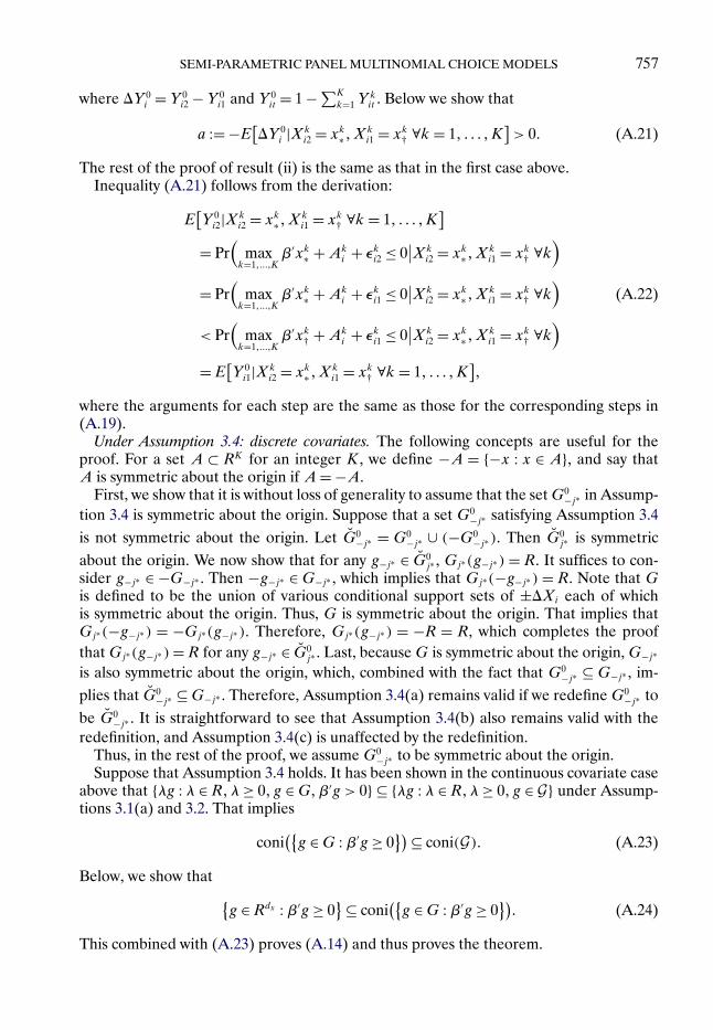
SEMI-PARAMETRIC PANEL MULTINOMIAL CHOICE MODELS 757

where �Y 0i = Y 0

i2 −Y 0i1 and Y 0

it = 1 − ∑K

k=1 Ykit . Below we show that

a := −E[�Y 0

i |Xki2 = xk

∗�Xki1 = xk

† ∀k= 1� � � � �K]> 0� (A.21)

The rest of the proof of result (ii) is the same as that in the first case above.Inequality (A.21) follows from the derivation:

E[Y 0

i2|Xki2 = xk

∗�Xki1 = xk

† ∀k = 1� � � � �K]

= Pr(

maxk=1�����K

β′xk∗ +Ak

i + εki2 ≤ 0∣∣Xk

i2 = xk∗�X

ki1 = xk

† ∀k)

= Pr(

maxk=1�����K

β′xk∗ +Ak

i + εki1 ≤ 0∣∣Xk

i2 = xk∗�X

ki1 = xk

† ∀k)

(A.22)

< Pr(

maxk=1�����K

β′xk† +Ak

i + εki1 ≤ 0∣∣Xk

i2 = xk∗�X

ki1 = xk

† ∀k)

= E[Y 0

i1|Xki2 = xk

∗�Xki1 = xk

† ∀k= 1� � � � �K]�

where the arguments for each step are the same as those for the corresponding steps in(A.19).

Under Assumption 3.4: discrete covariates. The following concepts are useful for theproof. For a set A ⊂ RK for an integer K, we define −A = {−x : x ∈ A}, and say thatA is symmetric about the origin if A = −A.

First, we show that it is without loss of generality to assume that the set G0−j∗ in Assump-

tion 3.4 is symmetric about the origin. Suppose that a set G0−j∗ satisfying Assumption 3.4

is not symmetric about the origin. Let G0−j∗ = G0

−j∗ ∪ (−G0−j∗). Then G0

j∗ is symmetricabout the origin. We now show that for any g−j∗ ∈ G0

j∗ , Gj∗(g−j∗) = R. It suffices to con-sider g−j∗ ∈ −G−j∗ . Then −g−j∗ ∈ G−j∗ , which implies that Gj∗(−g−j∗) = R. Note that Gis defined to be the union of various conditional support sets of ±�Xi each of whichis symmetric about the origin. Thus, G is symmetric about the origin. That implies thatGj∗(−g−j∗) = −Gj∗(g−j∗). Therefore, Gj∗(g−j∗) = −R = R, which completes the proofthat Gj∗(g−j∗)=R for any g−j∗ ∈ G0

j∗ . Last, because G is symmetric about the origin, G−j∗

is also symmetric about the origin, which, combined with the fact that G0−j∗ ⊆ G−j∗ , im-

plies that G0−j∗ ⊆G−j∗ . Therefore, Assumption 3.4(a) remains valid if we redefine G0

−j∗ tobe G0

−j∗ . It is straightforward to see that Assumption 3.4(b) also remains valid with theredefinition, and Assumption 3.4(c) is unaffected by the redefinition.

Thus, in the rest of the proof, we assume G0−j∗ to be symmetric about the origin.

Suppose that Assumption 3.4 holds. It has been shown in the continuous covariate caseabove that {λg : λ ∈ R�λ ≥ 0� g ∈ G�β′g > 0} ⊆ {λg : λ ∈ R�λ ≥ 0� g ∈ G} under Assump-tions 3.1(a) and 3.2. That implies

coni({g ∈ G : β′g ≥ 0

}) ⊆ coni(G)� (A.23)

Below, we show that {g ∈ Rdx : β′g ≥ 0

} ⊆ coni({g ∈G : β′g ≥ 0

})� (A.24)

This combined with (A.23) proves (A.14) and thus proves the theorem.

758 X. SHI, M. SHUM, AND W. SONG

Now we show (A.24). Suppose without loss of generality that βj∗ > 0. Let G0 = {g ∈Rdx : g−j ∈ G0

−j� gj∗ >−β′−j∗g−j∗/βj∗ }, where β−j∗ = (β1� � � � �βj∗−1�βj∗+1� � � � �βdx)

′. By As-sumption 3.4(a), we have that

G0 ⊆ {g ∈G : β′g ≥ 0

}� (A.25)

Consider an arbitrary point g0 ∈ {g ∈ Rdx : β′g ≥ 0}. Then, g0�j∗ > −g′0�−j∗β−j∗/βj∗ . That

means

d := g0�j∗ + g′0�−j∗β−j∗/βj∗ > 0� (A.26)

By Assumption 3.4(b), G0−j∗ spans Rdx−1, and is symmetric about the origin. Thus, G0

−j∗

spans Rdx−1 with nonnegative weights. Then, there exists a positive integer M , weightsc1� � � � � cM > 0, and g1�−j∗� � � � � gM�−j∗ ∈G0

−j∗ such that g0�−j∗ = ∑M

m=1 cmgm�−j∗ .Let gm�j∗ = (d/

∑M

m=1 cm) − (g′m�−j∗β−j∗/βj∗) for m = 1� � � � �M . Let gm be the vec-

tor whose j∗th element is gm�j∗ and which with the j∗ element removed is gm�−j∗ , form = 1� � � � �M . Then gm ∈ G0 for m = 1� � � � �M because gm�−j∗ ∈ G0

−j by construction andgm�j∗ > −g′

m�−j∗β−j∗/βj∗ due to d > 0. Also, it is easy to verify that g0 = ∑M

m=1 cmgm. Thus,g0 ∈ coni(G0). Subsequently, by (A.25),

g0 ∈ coni({g ∈ G : β′g ≥ 0

})� (A.27)

Therefore, (A.24) holds. Q.E.D.

PROOF OF THEOREM 4.1: For any b ∈ Rdx , let ‖b‖∞ = maxj=1�����J |bj|. Below, we showthat

β →p β/‖β‖∞� (A.28)

This implies that β →p β because β= β/‖β‖ and the mapping f : {b ∈Rdx : ‖b‖∞ = 1} →{b ∈Rdx : ‖b‖ = 1} such that f (b) = b/‖b‖ is continuous.

Now we show equation (A.28). Let

Q(b) =E[b′(�Xi)

(�p(Xi1�Xi2)

)]−� (A.29)

Under Assumption 3.1, the identifying inequalities (3.7) hold, which implies that

Q(β) = Q(β/‖β‖∞

) = 0� (A.30)

Consider any b such that ‖b‖∞ = 1 and b �= β/‖β‖∞. We have b/‖b‖ �= β/‖β‖ because thefunction f (b) = b/‖b‖ : {b ∈ Rdx : ‖b‖∞ = 1} → {b ∈ Rdx : ‖b‖ = 1} is one-to-one. Thus,for such a b, Theorem 3.1 implies that

Q(b) > 0� (A.31)

This, the continuity of Q(b), and the compactness of the parameter space {b ∈ Rdx :‖b‖∞ = 1} together imply that, for any constant c > 0, there exists a δ > 0 such that

infb∈Rdx :‖b‖∞=1�‖b−β‖>c

Q(b) ≥ δ� (A.32)

SEMI-PARAMETRIC PANEL MULTINOMIAL CHOICE MODELS 759

Next, we show the uniform convergence of Qn(b) to Q(b). Combining (A.31) and theuniform convergence, one can show the consistency of β using standard consistency ar-guments in, for example, Newey and McFadden (1994).

Now we show the uniform convergence of Qn(b) to Q(b). That is, we show that

supb∈Rdx :‖b‖∞=1

∣∣Q(b)−Qn(b)∣∣ →p 0� (A.33)

First, we show the stochastic equicontinuity of Qn(b). For any b�b∗ ∈ Rdx such that‖b‖∞ = ‖b∗‖∞ = 1, consider the following derivation:∣∣Qn(b)−Qn

(b∗)∣∣

≤ n−1n∑

i=1

∣∣(b− b∗)′(�Xi)

(�p(Xi1�Xi2)

)∣∣(A.34)

≤ n−1n∑

i=1

∥∥b− b∗∥∥∥∥(�Xi)(�p(Xi1�Xi2)

)∥∥≤ n−1

n∑i=1

‖�Xi‖∥∥b− b∗∥∥�

Therefore, for any fixed ε > 0, we have

limδ↓0

lim supn→∞

Pr(

supb�b∗∈Rdx �‖b‖∞=‖b∗‖∞=1�‖b−b∗‖≤δ

∣∣Qn(b)−Qn

(b∗)∣∣> ε

)

≤ limδ↓0

lim supn→∞

Pr

(δn−1

n∑i=1

‖�Xi‖> ε

)(A.35)

≤ limδ↓0

lim supn→∞

Pr

(n−1

n∑i=1

‖�Xi‖> ε/δ

)= 0�

where the first inequality holds by (A.34) and the equality holds by Assumption 4.1(b).This shows the stochastic equicontinuity of Qn(b).

Given the stochastic equicontinuity Qn(b) and the compactness of {b ∈ Rdx : ‖b‖∞ = 1},to show (A.33), it suffices to show that for all b ∈ Rdx : ‖b‖∞ = 1, we have

Qn(b) →p Q(b)� (A.36)

For this purpose, let

Qn(b) = n−1n∑

i=1

[(b′�Xi

)(�p(Xi1�Xi2)

)]−� (A.37)

By Assumption 4.1(b) and the law of large numbers, we have Qn(b) →p Q(b). Nowwe only need to show that |Qn(b) − Qn(b)| →p 0. But that follows from the deriva-

760 X. SHI, M. SHUM, AND W. SONG

tion: ∣∣Qn(b)−Qn(b)∣∣

≤ n−1n∑

i=1

∣∣(b′�Xi

)(�p(Xi1�Xi2)−�p(Xi1�Xi2)

)∣∣(A.38)

≤(

supi=1�����n

∥∥�pt(Xi1�Xi2)−�pt(Xi1�Xi2)∥∥)(

n−1n∑

i=1

∥∥b′Xi1 − b′Xi2

∥∥)→p 0�

where the convergence holds by Assumptions 4.1(a) and (b). Therefore, the theorem isproved. Q.E.D.

REFERENCES

ABREVAYA, J. (2000): “Rank Estimation of a Generalized Fixed-Effects Regression Model,” Journal of Econo-metrics, 95, 1–23. [738]

AHN, H., H. ICHIMURA, J. POWELL, AND P. RUUD (2018): “Simple Estimators for Invertible Index Models,”Journal of Business and Economic Statistics, 36, 1–10. [738,744]

ANDREWS, D., AND X. SHI (2013): “Inference Based on Conditional Moment Inequalities,” Econometrica, 81,609–666. [746,747]

BERRY, S., AND P. HAILE (2014): “Identification in Differentiated Products Markets Using Market-LevelData,” Econometrica, 82, 1749–1797. [750]

BERRY, S., J. LEVINSOHN, AND A. PAKES (1995): “Automobile Prices in Market Equilibrium,” Econometrica,65, 841–890. [750]

BONTEMPS, C., T. MAGNAC, AND E. MAURIN (2012): “Set Identified Linear Models,” Econometrica, 80, 1129–1155. [746]

BROWNING, M. (1989): “A Nonparametric Test of the Life-Cycle Rational Expectation Hypothesis,” Interna-tional Economic Review, 30, 979–992. [738]

CHAMBERLAIN, G. (1980): “Analysis of Variance With Qualitative Data,” Review of Economic Studies, 47, 225–238. [747]

(2010): “Binary Response Models for Panel Data: Identification and Information,” Econometrica, 78,159–168. [744]

CHERNOZHUKOV, V., S. LEE, AND A. ROSEN (2013): “Intersection Bounds: Estimation and Inference,” Econo-metrica, 81, 667–737. [746]

DEVROYE, L. P. (1978): “The Uniform Convergence of Nearest Neighbor Regression Function Estimators andTheir Applications in Optimization,” IEEE Transactions on Information Theory, IT-24, 142–151. [746]

FOX, J. (2007): “Semi-Parametric Estimation of Multinomial Discrete-Choice Models Using a Subset ofChoices,” RAND Journal of Economics, 38, 1002–1029. [738]

FREYBERGER, J. (2015): “Asymptotic Theory for Differentiated Product Demand Models With Many Mar-kets,” Journal of Econometrics, 185, 162–181. [750]

FREYBERGER, J., AND J. HOROWITZ (2015): “Identification and Shape Restrictions in Nonparametric Instru-mental Variables Estimation,” Journal of Econometrics, 189, 41–53. [746]

HAN, A. (1987): “Nonparametric Analysis of a Generalized Regression Model,” Journal of Econometrics, 35,303–316. [745]

HANSEN, B. E. (2008): “Uniform Convergence Rates for Kernel Estimation With Dependent Data,” Econo-metric Theory, 24, 726–748. [746]

HIRANO, K., G. W. IMBENS, AND G. RIDDER (2003): “Efficient Estimation of Average Treatment Effects Usingthe Estimated Propensity Score,” Econometrica, 71, 1161–1189. [746]

HODERLEIN, S., AND H. WHITE (2012): “Nonparametric Identification in Nonseparable Panel Data ModelsWith Generalized Fixed Effects,” Journal of Econometrics, 168, 300–314. [744]

HONORÉ, B., AND E. KYRIAZIDOU (2000): “Panel Discrete Choice Models With Lagged Dependent Vari-ables,” Econometrica, 68, 839–874. [738]

SEMI-PARAMETRIC PANEL MULTINOMIAL CHOICE MODELS 761

HONORÉ, B., AND A. LEWBEL (2002): “Semi-Parametric Binary Choice Panel Data Models Without StrictlyExogenous Regressors,” Econometrica, 70, 2053–2063. [738]

HOROWITZ, J. (2009): Semi-Parametric and Nonparametric Methods in Econometrics (Second Ed.).Springer. [739]

KHAN, S., AND E. TAMER (2009): “Inference on Endogenously Censored Regression Models Using Condi-tional Moment Inequalities,” Journal of Econometrics, 152, 104–119. [746,747]

KHAN, S., F. OUYANG, AND E. TAMER (2016): “Adaptive Rank Inference in Semiparametric Multinomial Re-sponse Models,” Working Paper. [738]

KIM, J., AND D. POLLARD (1990): “Cube Root Asymptotics,” Annals of Statistics, 18, 191–219. [751]KONING, R. H., AND G. RIDDER (2003): “Discrete Choice and Stochastic Utility Maximization,” Econometric

Journal, 6, 1–27. [749]LEWBEL, A. (1998): “Semi-Parametric Latent Variable Estimation With Endogenous or Mismeasured Regres-

sors,” Econometrica, 66, 105–121. [738](2000): “Semi-Parametric Qualitative Response Model Estimation With Unknown Heteroscedastic-

ity or Instrumental Variables,” Journal of Econometrics, 97, 145–177. [738]MANSKI, C. F. (1975): “Maximum Score Estimation of the Stochastic Utility Model,” Journal of Econometrics,

3, 205–228. [738,745](1987): “Semi-Parametric Analysis of Random Effects Linear Models From Binary Panel Data,”

Econometrica, 55, 357–362. [738,741,742,744]MCFADDEN, D. L. (1978): “Modeling the Choice of Residential Location,” in Spatial Interaction Theory and

Residential Location, ed. by A. Karlgvist et al. North-Holland. [740](1981): “Economic Models of Probabilistic Choice,” in Structural Analysis of Discrete Data With

Econometric Applications, ed. by C. Manski and D. McFadden. MIT Press. [740]NEWEY, W. K., AND D. L. MCFADDEN (1994): “Chapter 36 Large Sample Estimation and Hypothesis Testing,”

in Handbook of Econometrics, Vol. 4, ed. by R. F. Engle and D. L. McFadden. Elsevier. [759]PAKES, A., AND J. PORTER (2013): “Moment Inequalities for Semi-Parametric Multinomial Choice With Fixed

Effects,” Working Paper, Harvard University. [738,741]POWELL, J., AND P. RUUD (2008): “Simple Estimators for Semi-Parametric Multinomial Choice Models,”

Working Paper. [738]ROCKAFELLAR, R. T. (1970): Convex Analysis. Princeton Mathematical Series, No. 28. Princeton, NJ: Princeton

University Press. [739]SHERMAN, R. (1993): “The Limiting Distribution of the Maximum Rank Correlation Estimator,” Economet-

rica, 61, 123–137. [751]SHI, X., M. SHUM, AND W. SONG (2018): “Supplement to ‘Estimating Semi-Parametric Panel Multinomial

Choice Models Using Cyclic Monotonicity’,” Econometrica Supplemental Material, 86, https://doi.org/10.3982/ECTA14115. [744]

VILLANI, C. (2003): Topics in Optimal Transportation. American Mathematical Society, Graduate Studies inMathematics, Vol. 58. [739]

Co-editor Elie Tamer handled this manuscript.

Manuscript received 21 January, 2016; final version accepted 28 September, 2017; available online 18 October,2017.