Multinomial models

The multinomial distribution is a generalization of thebinomial distribution, for categorical variables with morethan two response types. In a multinomial randomexperiment, each single trial results in one of outcomes.5For instance, sampling with replacement from a populationwith types of individuals (like a bowl containing balls of55 different colors) is a multinomial random experiment.

types5

sample æ 8

with replacement æ

æ

The multinomial distribution is a probability model for thecounts resulting from such an experiment. Let:

1" œ æproportion of type 1 ( ) in the bowl1# œ proportion of type 2 ( ) in the bowl ã15 œ 5proportion of type ( ) in the bowl

The 's are (parameters) in the distribution, and14 constantsthey sum to 1:

1 1 1" # 5 ⠜ 1.

A multinomial experiment occurs when we independentlysample objects from the bowl with replacement, and8record the type of each one. Let:

] œ æ" number of type 1 ( ) in the sample] œ# number of type 2 ( ) in the sample ã] œ 55 number of type ( ) in the sample

The counts , , , are . They] ] á ]" # 5 random variablestake integer values between 0 and inclusive, but they8must also add to :8

] ] â ] œ 8" # 5 .

The 's are : the value of one affects the others.]4 dependentThe multinomial distribution is the multivariate (or joint)probability distribution for the random variables , , ,] ] á" #

]5:

T ] œ C ] œ C â ] œ C " " # # 5 5 and and and

,œ â8xC xC xâC x " #

C C C5" # 5

" # 51 1 1

where , , ..., are any nonnegative integers that add toC C C" # 8

8 (all possible outcomes). We write

] ] á ] 8 á" # 5 " # 5, , , ~ multinomial( , , , , ) .1 1 1

The binomial distribution is a special case corresponding to5 œ # ] œ 8 ]. In this case, the number of failures is .# "

Example. In political polling, each voter selected for thesample is categorized into one of mutually exclusive5categories. For instance, in a random sample of voters in8the USA,

] œ" # democrats,] œ# # republicans,] œ$ # independents (no party),] œ4 # “other” (libertarians, greens, etc).

The counts , , , are random variables, in that if] ] ] ]" # $ 4

the poll were to be repeated (a new sample of voters8selected) the counts would likely be somewhat different.Note that political polling and other such surveys aregenerally done by sampling without replacement.However, the multinomial model will be a goodapproximation to the distribution of the counts provided thechanges in the proportions in the population (the 's) due14

to sampling are negligible. (The exact distribution of thecounts for sampling without replacement is called themultivariate hypergeometric distribution).

Properties of the multinomial distribution

E ] œ 84 41

V ] œ 8 " 4 4 41 1

Cov ( ] ] œ 3 Á 4Ñ3 4 3 41 1

Also, an important property of the multinomial distributionis that any subgroup of the 's, conditional on their sum,]4

has a multinomial distribution. For instance,

] ] ] l Ð] ] ] œ 7Ñ µ" # $ " # $, ,

multinomial( , , , ) ,7 : : :" # $

where .: œ Î 3 3 " # $1 1 1 1 Another important property is that any subgroup of the 's]4

can be pooled (summed) into one count, and the resultingcollection of counts has a multinomial distribution, with theproportion for the new pooled category being the sum ofthe original probabilities for the counts being pooled. Aspecial case of this property is that the marginal distributionof a single count is binomial:

] µ 84 4binomial( , ) .1

In this case, the number of failures is the sum of all thecounts for the other categories.

Saturated parameter model

The multinomial distribution is called “saturated” if all ofthe population proportions , , , have unknown1 1 1" # 5ávalues. This translates to free unknown parameters,5 "

because knowing the values of of the proportions5 "provides the value of the remaining proportion due to theconstraint that the proportions sum to ."

Suppose a multinomial experiment has been conducted.The data are the resulting counts, , , ..., , and theC C C" # 5

“sample size” is the number of trials . The likelihood8function for the unknown parameters is

P á œ â 1 1 1 1 1 1" # 58x

C xC xâC x " #C C C

5, , , ," # 5

" # 5

and the log-likelihood is

log log log . P œ C8xC xC xâC x

4œ"

5

4 4" # 5

1

The maximum likelihood (ML) estimates , , ..., are1 1 1s s s" # 5

the values of , , , that jointly maximize or1 1 1" # 5á Plog , subject to the constraint that P á 1 1 1" # 5

œ ". The constrained maximization has a symbolicsolution that can be derived, for instance, with theLagrange multiplier technique from calculus. The resultingsolution is intuitive; the ML estimates are simply thesample proportions of the categories:

1s œ4C84 .

The ML estimate for the mean of is found from :] s4 41

E .s ] œ 8 œ Cs 4 4 41

Now E is the prediction for a new value of under thes ] ] 4 4

model, and the predictions fit all the observed counts C4perfectly. The model has as many unknown parameters asfree data points, hence the characterization of the model as“saturated.”

One must be careful of terminology with the multinomialmodel when speaking about “sample size.” The number ofraw observations (each a single event, categorized into oneof categories) is . The number of counts is , of which5 8 55 " are nonsingular random variables.

Reduced-parameter models

The saturated multinomial model has 1 unknown free5 parameters for describing free counts. An5 "interesting, and scientifically useful, class of multinomialmodels arise when the 's are constructed as functions of14

fewer underlying parameters. Many different functionsarise out of various scientific mechanisms.

Examples of reduced-parameter models

1. Hardy-Weinberg equilibrium

Genes of two types (alleles), denoted A, a, present in apopulation at a location (locus) on a chromosome pair.Possible genotypes are AA, Aa, aa.

Bucket of gametes:

A A a a A a A a A A a A A

Gene proportions: proportion of A: œ 1 proportion of a : œ

Random mating with no selection is like drawing twoalleles at random (with replacement) from the bucket tomake a new individual:

AAT œ : #

Aa 2 1 “Hardy-Weinberg proportions”T œ : : aa 1T œ : #Draw sample of individuals in population; determine8their genotypes (AA, Aa, or aa). #AA, #Aa,] œ ] œ" #

] œ$ #aa in sample.

Model: , , multinomial , , ] ] ] µ 8ß" # $ " # $ 1 1 1

where 1"#œ :

2 11# œ : : 11$

#œ : This is a multinomial model with one unknown parametergiven by .:

Question for thought: suppose the counts resulting fromsampling individuals are denoted by , , . What is8 C C C" # $

the ML estimate for ?:

2. Bird-banding

Capture (usually by mist netting) and band adult birds,8and release them back into the wild.

prob. of surviving a given yr< œ prob. that band is found & returned (given the= œ bird dies) in the year of death

Study lasts for three years; # band returns in first yr,] œ"

#band returns in second yr, # band returns] œ ] œ# $

in third yr, # birds with unreturned bands.] œ%

Model: , , , multinomial , , , , ] ] ] ] µ 8" # $ % " # $ % 1 1 1 1

11" œ < = 11# œ < < = 11$

#œ < < = 1 1 1 11%

#œ < = < < = < < = Model has two unknown parameters and < =

3. Fitting a probability distribution to grouped data

The multinomial distribution is used for fitting probabilitydistributions to data grouped into frequency counts.Suppose the set of real numbers is separated into 5

intervals, with boundaries of known values given by , ,= =" #

..., . The boundaries are typically chosen by the=5"

investigator, but occasionally the boundaries are given bythe scientific problem.

As an example, suppose , , ..., represent a random\ \ \" # 8

sample drawn from a from a normal , distribution. . 5#

Suppose also that these raw observations are grouped intointerval categories, with the frequency counts representedby ] ] á ]" # 5, , , :

] œ ∞ =" "# of observations in , ] œ = =# " ## of observations in , ] œ = =$ # $# of observations in , ã] œ = =5" 5# 5"# of observations in , ] œ = ∞5 5"# of observations in , The probabilities corresponding to these frequency countsare given by areas under a normal , curve: . 5#

1" "œ ∞ =area under normal curve from to 1# " #œ = =area under normal curve from to ã15 5"œ = ∞area under normal curve from to

The multinomial model for the 's has unknown]4 twoparameters: and .. 5#

Notes on picking boundaries: Setting the boundaries atvalues that cannot actually occur in the sample avoids the

need for specifying rules for categorizing an observationthat lands on a border. For instance, one can defineboundary values that have a greater number of decimalplaces than the precision of the raw observations. Fordiscrete distributions defined on the integers, one can setthe boundaries at half-integer values. Also, for adequateasymptotics (for the parameter estimates and the chisquaregoodness of fit test), the intervals should be formed so asnot to have low expected counts. The intervals do not haveto be equal in width; rather, intervals roughly equal inexpected frequency are better. Finally, to assure that thefrequency counts have a multinomial distribution, theintervals should partition the entire sample space, so thatevery potential raw observation can be categorized into oneof mutually exclusive categories.5

Maximum likelihood estimation for reduced parametermultinomial models

We write the general reduced parameter model as

] ] á ] 8 á" # 5 " # 5, , , ~ multinomial( , , , , ) ,1 1 1

where the 's can be represented as functions of fewer14

underlying parameters (let's call the underlying parameters) ) )" # 6, , ..., , with ):6 Ÿ 5 "

1 ) ) )" " " # 6œ 1 , , ..., 1 ) ) )# # " # 6œ 1 , , ..., ã1 ) ) )5 5 " # 6œ 1 , , ...,

The data are the counts resulting from aC C C" # 5, , ..., sample of size . The ML estimates of , , ..., are the8 ) ) )" # 6

values, say , , ..., , that jointly maximize the) ) )s s s" # 6

multinomial log-likelihood function given by

log log log P œ C 18xC xC xâC x

4œ"

5

4 4" # 5

) ) )" # 6, , ..., .

Numerical maximization is required for all but the simplestapplications (such as the genetic H-W equilibrium, above).Interestingly, many computer packages for nonlinear leastsquares (SAS PROC NLIN, etc.) can be “tricked” intomaximizing a multinomial likelihood instead of minimizinga sum of squares. The trick uses the counts C C C" # 5, , ..., asthe observations of the “response variable” and thecorresponding expected counts given by E ] œ4

814 ) ) )" # 6, , ..., , , , ..., as the regression model to4 œ " # 5be fit. The ordinary least squares estimates are the MLnotestimates for the multinomial; the trick is to weight eachobservation by , , ..., and update the value"Î 814 ) ) )" # 6

of the weight with the new parameter values each iterationof the Gauss-Newton sum of squares algorithm. The“_WEIGHT_” statement in SAS PROC NLIN wasdesigned for such use. Because the multinomial expectedvalues typically are functionally different for eachobservation, the regression model form has to be specifiedseparately for each observation by means of a series of “IF”statements. This “iteratively reweighted least squares”algorithm converges to the ML estimates for the

multinomial model, and the corresponding “weighted sumof squares” is the Pearson chisquare goodness of fitstatistic. Furthermore, if the asymptotic variance-covariance matrix from the nonlinear regression isevaluated using (where is the variance parameter5 5# #œ "in the nonlinear regression), the result is the correctasymptotic variance-covariance matrix for the parametersof the multinomial model that arise from the Fisherinformation matrix. The “SIGSQ ” option in the PROCœ "NLIN statement of SAS accomplishes the appropriatescaling of the variance covariance matrix for multinomialmodels.

Goodness of fit test for a reduced parametermultinomial model

The multinomial goodness of fit test is a statistical test of aspecified reduced parameter model against a saturatedmodel. The null hypothesis is a reduced parametermultinomial model for describing the 's, that is, the 's]4 41can be represented in terms of fewer underlying parameters( , , ..., ):) ) )" # 6

H : , , ..., ! " " " # 61 ) ) )œ 1 , , ..., 1 ) ) )# # " # 6œ 1 ã , , ..., 1 ) ) )5 5 " # 6œ 1 Note: in goodness of fit tests, the null hypothesis is oftenthe “research model” of interest.

The alternative hypothesis is that a more complex,unspecified multinomial model is necessary to describe the] 5 4 " # 5"'s, that is, all 1 free parameters , , ..., are1 1 1needed to describe the data adequately:

H : " " "1 1œ 1 1# #œ ã 1 15" 5"œ

Here H is the ordinary saturated multinomial. In situations1

where the null model is the research hypothesis (i.e. themodel for which the researcher seeks to convince a skepticof its merits), the alternative hypothesis becomes theskeptic's hypothesis. The skeptic would claim that the nullhypothesis model is too simple a mechanism for producingthe data.

The data are the counts , , ..., . To perform theC C C" # 5

statistical test, one must calculate ML estimates for the nullhypothesis model (usually using numerical maximization).The resulting maximized likelihood value, , is evaluatedPs!

as

P œs!

8xC xC xâC x " #

C C C5" # 5

" # 51 1 1~ ~ ~ .â

where , , ..., .~1 ) ) )4 4 " # 6œ 1 s s s

Similarly, the likelihood evaluated at the ML estimates forthe alternative hypothesis is

P œs"

8xC xC xâC x " #

C C C5" # 5

" # 51 1 1s s sâ

where . The likelihood ratio statistic for testing H1s œ4 !C84

versus H becomes"

K œ # Ps

Ps2 log . !

"

For these multinomial models, the likelihood ratio statisticalgebraically reduces to a simpler form, requiringcalculation only of the ML estimates and expected valuesunder H . Let (ML-estimated expected value~

! 4 4I œ 8s 1of under the null hypothesis). The likelihood ratio]4

goodness of fit statistic for the multinomial reduces to

K œ C#

4œ"

5

4C

Is2 log . 4

4

This is in the form 2 observed log .D observedestimated expected

Also, one can show by asymptotic expansion that

K ¸ œ \# #

4œ"

5 C Is

Is 4 4

#

4

,

that is, (likelihood ratio statistic) and Pearson'sK#

chisquare statistic are asymptotically similar.

If the data arise from the null hypothesis model, then K#

and both have approximate chisquare distributions with\#

5 " 6 df (# parameters estimated in alternative modelminus # parameters estimated in null model). One rejectsH in favor of H if , where the chisquare! "

# #K   ;αpercentile corresponds to 1 df. One concludes that5 6 the null model “fits” if .K # #;α

In ordinary analysis of variance tests, the skeptic'shypothesis is usually the null model and the researchhypothesis is the alternative. In goodness of fit tests, thenull/alternative configuration of the skeptic's and researchhypotheses is often reversed. As such, support for theresearch hypothesis in goodness of fit takes the form of“failure to reject the null hypothesis” and is thereby aweaker statement than rejection of the null in favor of thealternative. Acceptance of goodness of fit means only thatthe data are a plausible realization of the null model; itdoes not mean that the null model (or some approximationthereof) necessarily generated the data.

Goodness of fit is an important ingredient of modelevaluation, but it is not the only ingredient. A statisticalmodel ultimately is a scientific hypothesis that purports toexplain how numerical observations arise, and evaluatingthe model's reliability as a predictive tool and as asupporting strand in a web of other scientific hypothesesrequires further evidence. One might think of goodness offit as scientifically necessary, but not scientificallysufficient.

Examples of goodness of fit tests

1. Are human blood types in H-W proportions?

3 alleles A, B, O with proportions , , in population+ , 9(where ; there are unknown parameters)+ , 9 œ " two

genotypes phenotypes frequencies (H-W)

type A 2AAAO 1"

#œ + +9

type B 2BBBO 1#

#œ , ,9

AB type AB 21$ œ +,

OO type O 1%#œ 9

Data (from Rao CR. 1973. Linear Statistical Inference andits Applications. Wiley): 182, 60, 17,C œ C œ C œ" # $

C œ 8 œ% 176, 435

ML estimates under H : H-W proportions!

(computer maximization of ):P!

0.2644485+ œs

0.09319721, œs

0.64235439 œs

log 9.096694 P œ s!

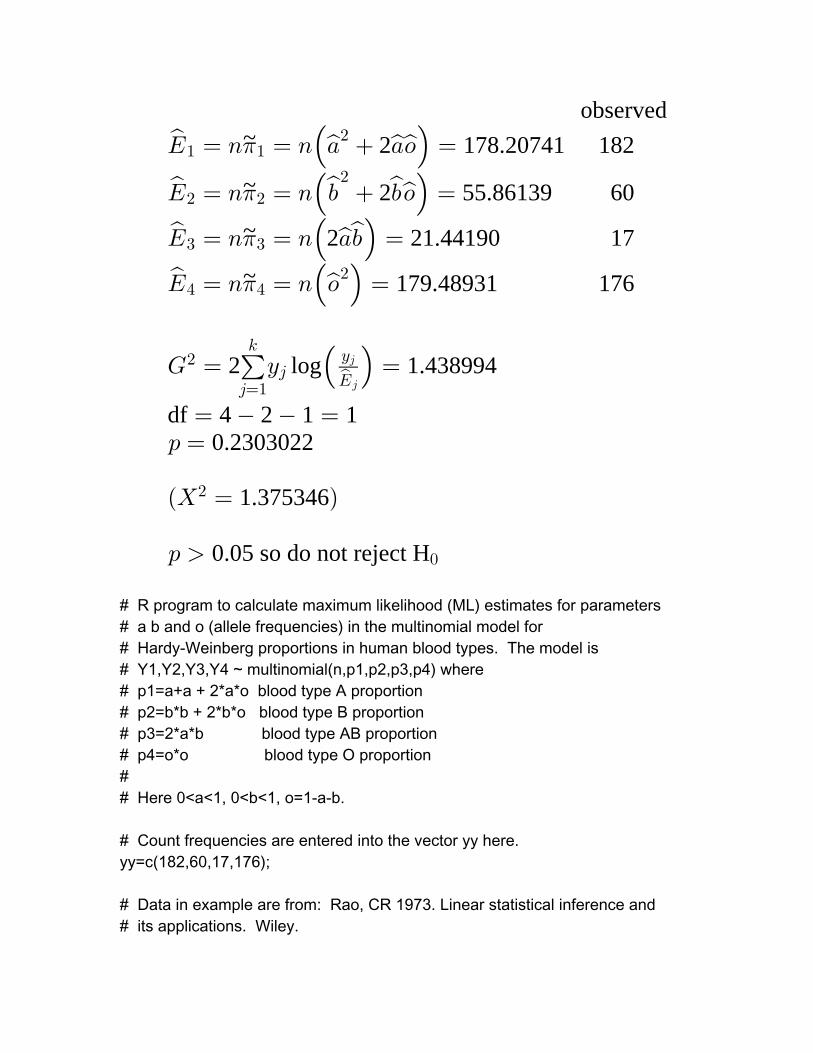
observed

2 178.20741 182~I œ 8 œ 8 + +9 œs s ss" "#

1 2 55.86139 60~I œ 8 œ 8 , ,9 œs s ss# #

#1

2 21.44190 17~I œ 8 œ 8 +, œs ss$ $1 179.48931 176~I œ 8 œ 8 9 œs s% %

#1

2 log 1.438994K œ C œ#

4œ"

5

4C

Is 4

4

df 4 2 1 1œ œ 0.2303022: œ

1.375346 \ œ#

0.05 so do not reject H: !

# R program to calculate maximum likelihood (ML) estimates for parameters# a b and o (allele frequencies) in the multinomial model for# Hardy-Weinberg proportions in human blood types. The model is# Y1,Y2,Y3,Y4 ~ multinomial(n,p1,p2,p3,p4) where# p1=a+a + 2*a*o blood type A proportion# p2=b*b + 2*b*o blood type B proportion# p3=2*a*b blood type AB proportion# p4=o*o blood type O proportion## Here 0<a<1, 0<b<1, o=1-a-b.

# Count frequencies are entered into the vector yy here.yy=c(182,60,17,176);

# Data in example are from: Rao, CR 1973. Linear statistical inference and# its applications. Wiley.

# Set initial patameter values here.a0=.33;b0=.33;

# ML objective function "negloglike.ml" is negative of log-likelihood;# the Nelder-Mead optimization routine in R, "optim", is a minimization# routine. The two function arguments are: theta = vector of# parameters (transformed to real line), ys = vector of frequencies.

negloglike.ml=function(theta,ys){ a=exp(-exp(theta[1])); # Constrains 0 < a < 1. b=exp(-exp(theta[2])); # Constrains 0 < b < 1. o=1-a-b; n=sum(ys); k=length(ys); p=c( a*a+2*a*o, b*b+2*b*o, 2*a*b, o*o ); # H-W model for the probabilities.

ofn=-sum(ys*log(p)); # No need to calculate all the factorials. return(ofn);}

# The ML estimates.MULTML=optim(par=c(log(-log(a0)),log(-log(b0))), negloglike.ml,NULL,method="Nelder-Mead",ys=yy);reslts=c(exp(-exp(MULTML$par[1])),exp(-exp(MULTML$par[2])),-MULTML$val);a.ml=reslts[1]; # These are the ML estimates.b.ml=reslts[2]; # --o.ml=1-a.ml-b.ml; # --

nn=sum(yy);loglike.ml=reslts[3]+lfactorial(nn)-sum(lfactorial(yy));

# Calculate expected values, LR statistic, etc.pp=c( a.ml*a.ml+2*a.ml*o.ml, b.ml*b.ml+2*b.ml*o.ml, 2*a.ml*b.ml,

o.ml*o.ml );EE=nn*pp;y1=yy;y1[y1==0]=1; # Guard against log(0) in G-squared.Gsq=2*sum(yy*log(y1/EE)); # G-squared goodness of fit statistic.pval=1-pchisq(Gsq,1);

# Print the results.a.ml;b.ml;o.ml;loglike.ml;Gsq;pval;cbind(EE,yy);

2. Do lodgepole pines have a Poisson spatial distribution?

100 quadrats placed at random in a lodgepole pine forest.\ œ # trees in a quadrat.

Poisson model: P , , , , ... \ œ B œ B œ ! " #/Bx

B--

Frequency counts:] œ !" # quadrats with trees] œ "# # quadrats with tree] œ #$ # quadrats with trees ã] œ 5 #5" # quadrats with trees] œ 5 "5 # quadrats with or greater trees

Multinomial distribution of frequency counts:

] ] ] µ 8" # 5 " # 5, , ..., multinomial( , , , ..., )1 1 1

where

1 -" "/!xœ \ œ ! œ œ 1P ( ) !--

1 -# #/"xœ \ œ " œ œ 1P ( etc.) "--

1$/#xœ \ œ # œP #--

ã15"

/5# xœ \ œ 5 # œP 5#--

1 1 1 15 " # 5"œ \   5 " œ " âP # trees per frequency estimated expected

quadrat ( ) count ( ) frequency ( )B C 81 s4 4 -

0 7 5.728991 1 16 16.382799 2 20 23.424378 3 24 22.328357 4 17 15.962714 5 9 9.129494 6 5 4.351164 7 2 2.692104 

-s œ 2.859631

log 13.97714 P œ s!

K œ : œ# 1.276895 0.2584772\ œ : œ# 1.260605 0.2615366

# R program to calculate maximum likelihood (ML) estimates for parameter# in the Poisson distribution using a multinomial likelihood for goodness of# fit test.# Here P[X=x] = exp(-lambda)(lambda^x)/(x!), x=0,1,2,... .# Data are pooled frequency counts:# y1 = #{X=0}, y2 = #{X=1},..., yk = #{X>=(k-1)}.

# Count frequencies are entered into the vector yy here. The last frequency# is the pooled tail counts.yy=c(7,16,20,24,17,9,5,2);

# Initial patameter value is calculated from the approximate sample mean.kk=length(yy);nn=sum(yy);xx=0:(kk-1);lambda0=sum(xx*yy)/nn;

# ML objective function "negloglike.ml" is negative of log-likelihood;# the optimization routine in R, "optim", is a minimization# routine. The two function arguments are: theta = parameter# (transformed to real line), ys = vector of frequencies.

negloglike.ml=function(theta,ys){ lambda=exp(theta); # Constrains 0 < lambda. k=length(ys); x=0:(k-1); x1=x[1:(k-1)]; p=rep(0,k); p[1:(k-1)]=exp(-lambda+x1*log(lambda)-lfactorial(x1)); p[k]=1-sum(p[1:(k-1)]); ofn=-sum(ys*log(p)); # No need to calculate all the factorials. return(ofn);}

# The ML estimate.MULTML=optim(par=log(lambda0), negloglike.ml,NULL,method="BFGS",ys=yy); # Nelder-Mead algorithm is not # reliable for 1-D problems.reslts=c(exp(MULTML$par[1]),-MULTML$val);

lambda.ml=reslts[1]; # This is the ML estimate.nn=sum(yy);loglike.ml=reslts[2]+lfactorial(nn)-sum(lfactorial(yy)); # Log-likelihood.

# Calculate expected values, LR statistic, etc.xx1=xx[1:(kk-1)];pp=rep(0,kk);pp[1:(kk-1)]=exp(-lambda.ml+xx1*log(lambda.ml)-lfactorial(xx1));pp[kk]=1-sum(pp[1:(kk-1)]);EE=nn*pp;y1=yy;y1[y1==0]=1; # Guard against log(0) in G-squared.Gsq=2*sum(yy*log(y1/EE)); # G-squared goodness of fit statistic.pvalG=1-pchisq(Gsq,1); # p-value (chisquare distribution) for G-squared.Xsq=sum((yy-EE)^2/EE); # Pearson goodness of fit statistic.pvalX=1-pchisq(Xsq,1); # p-value (chisquare distribution) for Pearson.

# Print the results.lambda.ml;loglike.ml;Gsq;pvalG;Xsq;pvalX;cbind(EE,yy);

Confidence intervals

1. . The curvature of the log-Wald confidence intervalslikelihood function near its peak describes how well thedata distinguish among different nearby parameter values.If the log-likelihood function is a narrow, steep peak, thencurvature is large and the data are providing goodinformation for estimating the parameter values. If the log-likelihood function slopes down from its peak only gently,a large range of parameter values provide a log-likelihoodvalue almost as high as that of the ML estimate, and the

data do not provide good information for parameterestimation.

Commonly used measures of the quality of estimation arebased on the log-likelihood curvature. The log-likelihoodcurvature is defined by the Hessian matrix of secondderivatives. The element in the th row and the th3 7column of the Hessian matrix is:

` P` ` 1 ` ` ` `

4œ"

5C ` 1 C `1 `1

1

#

3 7 4 3 7 3 7

4 4 4 4 4#

#4

log )) ) ) ) ) ) )

) ) )

)œ .

Here ) œ ( , , ..., ). In hypothetically repeated) ) )" # 6

samples, log and its derivatives are random variables.P )In particular, the elements of the Hessian matrix are linearfunctions of the mulinomial observations , , ..., , andC C C" # 5

their expected values can be found by substituting theexpected values , , ..., of the81 81 81" # 5 ) ) )observations The element in the th row and the thÞ 3 4column in the matrix of expected values of the secondderivatives is

E . ` P` ` 1 ` `

4œ"

5" `1 `1#

3 7 4 3 7

4 4log )) ) ) ) )

) )œ 8

The expression results from the fact that D )1 œ "4 thereby producing .D ) ) )` 1 Î ` ` œ !#

4 3 7 The essential curvature of the log-likelihood near itsmaximum is negative; a measure of the amount of

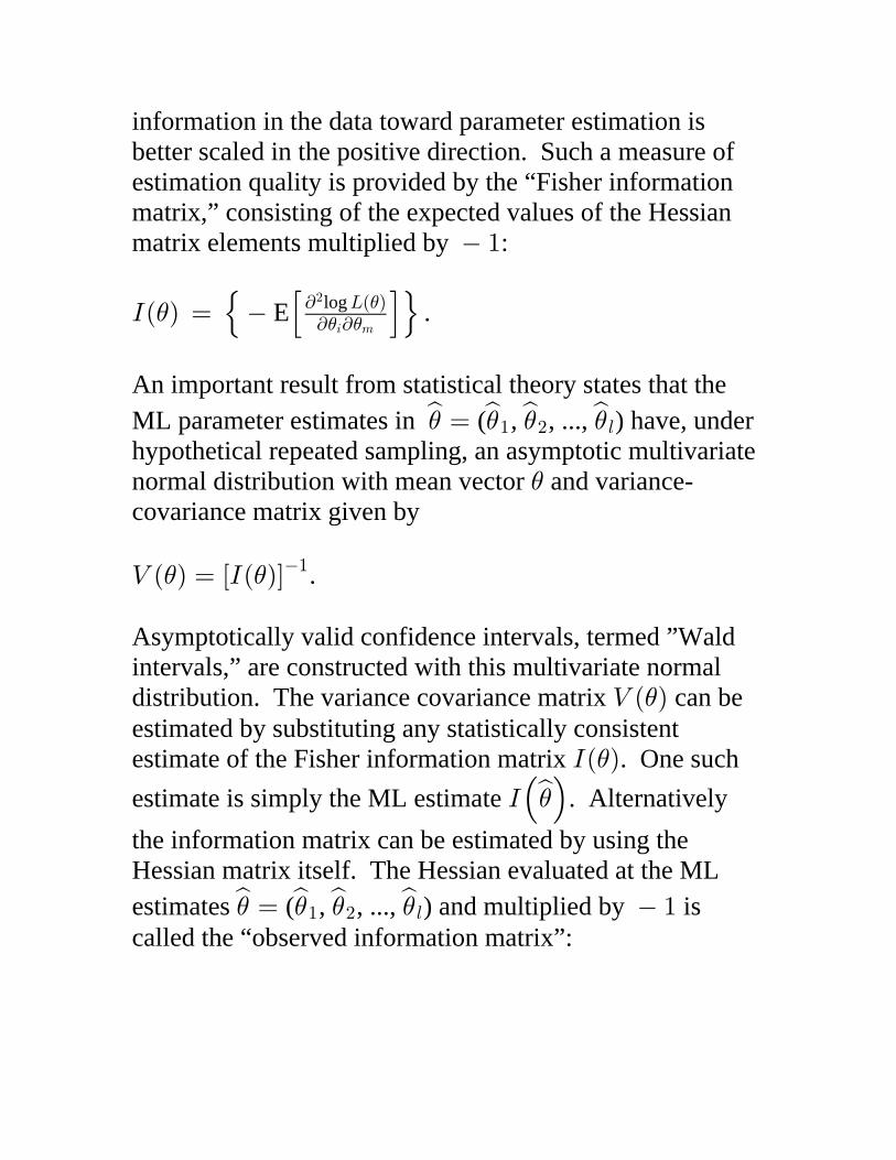
information in the data toward parameter estimation isbetter scaled in the positive direction. Such a measure ofestimation quality is provided by the “Fisher informationmatrix,” consisting of the expected values of the Hessianmatrix elements multiplied by : "

M œ ) E ` P` `

#

3 7

log )) ) .

An important result from statistical theory states that theML parameter estimates in ( , , ..., ))s œ ) ) )s s s

" # 6 have, underhypothetical repeated sampling, an asymptotic multivariatenormal distribution with mean vector and variance-)covariance matrix given by

Z œ M ) ) ".

Asymptotically valid confidence intervals, termed ”Waldintervals,” are constructed with this multivariate normaldistribution. The variance covariance matrix can beZ ) estimated by substituting any statistically consistentestimate of the Fisher information matrix M ) . One such

estimate is simply the ML estimate . AlternativelyM s )the information matrix can be estimated by using theHessian matrix itself. The Hessian evaluated at the MLestimates ( , , ..., ) and multiplied by is)s œ ) ) )s s s "" # 6

called the “observed information matrix”:

N œ )s` P s

` `

#

3 7

log )) ) .

Either or are statistically consistent M N) )s s" "

estimates of .Z )A Wald interval is an asymptotic % confidence"!!Ð" Ñαinterval for formed by)3

)s „ D @s3 33Î#α ,

where is the th percentile of a standardD "!! " Î#αÎ# α

normal distribution and is the th element in the main@ 3s33

diagonal of the estimated variance-covariance matrix .Zs )In practice, sample sizes are frequently not large enough toattain “asymptopia,” and actual coverage probabilities ofasymptotic confidence intervals can be considerablydifferent from the claimed probabilities. Wald intervals areknown to be often too small. Simulations suggest that

intervals using the observed information matrix tendN )sto have slightly better properties than those using the ML

Fisher infomation matrix M s ) , but actual details differ

from model to model.

2. . The key problem forBootstrap confidence intervalsconstricting a confidence interval for a parameter is to)3

estimate how variable its ML estimate is under)̂3hypothetical repeated sampling (the so-called sampling

distribution of ). Bootstrapping is a straightforward,)̂3computer-intensive appproach to “estimating the variabilityof estimation,” and is the statistical version of “pullingyourself up by your bootstraps.” The basic principle iseasy: obtain an estimate of the model, simulate thousandsof new data sets from the estimated model, and refit themodel to each of the new data sets. The resultingcollection of thousands of parameter values forms astatistically consistent estimate of the sampling distribution.

The estimated model in the present context is themultinomial distribution evaluated at the ML parameterestimates . One computer-generates multinomial data)s ,sets (say, ) from the estimated model and re-, œ "!ß !!!calculates ML parameter estimates for each data set. Eachbootstrap data set should have the same sample size as theoriginal data. The resulting bootstrap parameter estimates

) ) )s s sÐ"Ñ Ð#Ñ Ð,Ñ, , ..., can be treated as a huge sample from the

sampling distribution of . An asymptotic 95% confidence)s

interval for , for instance, is given by the empirical 2.5th)3and 97.5th percentiles of the bootstrap estimates of .)3

3. . A confidenceProfile likelihood confidence intervalsinterval can be constructed by inverting a two-sidedhypothesis test concerning the parameter in question. Thenull hypothesis is that the parameter is equal to a constantknown value:

H : .! 3 3!) )œ

The alternative hypothesis is that the parameter is anunknown constant:

H : ." 3 3!) )Á

A valid ( % confidence interval is the set of all"!! " Ñαvalues of for which the null hypothesis would not be)3!rejected, using a significance level of .α

A profile likelihood confidence interval for uses the)3generalized likelihood ratio test and the asymptoticchisquare distribution of the test statistic to form theconfidence interval. For a range of fixed values of , one)3maximizes the log-likelihood with respect to the remainingunknown parameters. Usually the process requires manynumerical maximizations, one for each new value of .)3Typically the maximized values of the log-likelihood areplotted versus the corresponding values, ideally resulting)3in a unimodal curve, like a rounded mountain. The summitof the curve represents log , the log-likelihoodPs"

maximized under the alternative hypothesis (full MLestimates of all parameters including ). The confidence)3interval is all the values for which the maximized log-)3likelihood is above a certain altitude on the peak. Thethreshold is given by the asymptotic chisquare distributionof the likelihood ratio test statistic. A valid asymptotic"!!Ð" Ñα )% confidence interval is the set of values for3

which

K œ # P P Ÿs s# #" ! log log ,;α

where the chisquare distribution has 1 df. For example, a*&% confidence interval is the set of values for which the)3height of the log curve is within a vertical distance ofPs!

;#αÎ# œ $Þ)%Î# œ "Þ*# from the summit.

Beyond its use for constructing confidence intervals, aprofile log-likelihood plot is a recommended ingredient ofmodel evaluation. A nearly flat or multimodal profile canwarn of estimability problems; different sets of parametersare producing similarly high log-likelihoods. An idealprofile looks parabolic. Many tough-to-estimateparameters (such as population size in mark recapturemodels) produce asymmetric profiles, with a steep declineon one side and gentle decline on the other, leading toconfidence intervals that are highly asymmetric around theML point estimate.

In general, decades of simulations of many models in thestatistical literature suggests that both bootstrap and profilelikelihood confidence intervals tend to perform better thanWald intervals. Neither bootstrap nor profile likelihoodintervals produce interval boundaries outside the range ofthe parameter, a phenomenon which can occur with Waldintervals (estimated survival probabilities less than zero,etc.). Bootstrap and profile likelihood intervals tend tohave actual coverage probabilities for moderate-sizedsamples that are adequately close to the claimed coverage

probabilities, while the actual Wald coverage probabilitiestend to be too small. Nonetheless, there are situations forwhich all three can be bad. Statistical theory gives a fewwarnings: a parameter at or near the edge of its range, arandom variable with a range that depends on an unknownmodel parameter, and sparse data are situations that cancause estimation problems. However, statistical theoryprovides no sweeping guidance for confidence intervalsacross model families; basically, each new model for eachnew application has to have its confidence intervals testedby simulation, for the conditions and sample sizes likely tobe encountered in practice. There will never be a shortageof topics for statistical masters degrees.