the ordered and multinomial models - uc3m - …ricmora/miccua/materials/s13t31_english...motivation...

MotivationOrdered Response Models

Multinomial ResponseSummary

The Ordered and Multinomial ModelsQuantitative Microeconomics

R. Mora

Department of Economics

Universidad Carlos III de Madrid

R. Mora Ordered & Multinomial



Outline

1 Motivation

2 Ordered Response Models

3 Multinomial Response




Motivation




We consider the following two extensions from binary dependentmodels:

Ordered response models: The dependent variable takes anumber of �nite and discrete values that contain ordinal

information.

Multinomial response models: The dependent variable takes anumber of �nite and discrete values that DO NOT containordinal information.

As in the probit and logit cases, the dependent variable is notstrictly continuous. Estimation will be carried out using the MLestimator.




Examples of ordered models

Credit rating, using seven categories, from �absolutely notcredit worthy� to �credit worthy�.

Decision to remain inactive, to work part-time, or to workfull-time.

In an income regression, income levels are coded in intervals:[0,1000), [1000,1500)[1500,2000),[2000,∞)

On value statements, several answers with ordinal content:�completely disagree�, �disagree�, �somewhat agree�,�completely agree�




Examples of multinomial models

Choice of transport mode: train, bus, car

Economic status: inactive, unemployed, self-employed,employee

Education �eld choice: hard science, health sciences, socialsciences, humanities




Ordered Response Models




The two standard models are the ordered probit and theordered logit.

The approach is equivalent: we simply use for the orderedprobit the normal CDF Φ() and for the ordered logit thelogistic CDf Λ().

OLS does not work because the dependent variable does nothave cardinal meaning:

credit worthiness: 0,1,2,3,4,5: the change from 0 to 1 doesnot have to be �equivalent� to the change from 4 to 5.activity: inactive=0, part-time=1, full-time=2: While inactiveis zero hours of work, in practice code 1 re�ects any hours ofwork between 1 and (usually) 30 hours of work, and code 2re�ects more 30 hours of work. This implies that there is noproportionality in going from 0 to 1 and going from 1 to 2.




Simpli�cation

Binary choice models (LPM, probit, logit) could potentially beused by grouping all categories into two major ones,

This is the case when the sample is small and the ordinalcategories can be logically be grouped in two major categories.

In some cases, this is probably a very bad idea (incomeintervals).




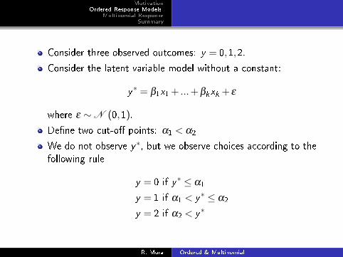
Consider three observed outcomes: y = 0,1,2.

Consider the latent variable model without a constant:

y∗ = β1x1 + ...+ βkxk + ε

where ε ∼N (0,1).

De�ne two cut-o� points: α1 < α2

We do not observe y∗, but we observe choices according to thefollowing rule

y = 0 if y∗ ≤ α1

y = 1 if α1 < y∗ ≤ α2

y = 2 if α2 < y∗




Example: activity

y = 0 if inactive, y = 1 if part-time, y = 2 if full-time

y∗ = βe × educ + βk ×kids + ε , where ε ∼N (0,1)

Then

y = 0 if βe × educ + βk ×kids + ε ≤ α1

y = 1 if α1 < βe × educ + βk ×kids + ε ≤ α2

y = 2 if α2 < βe × educ + βk ×kids + ε

Note that we could alternatively introduce a constant β0 andassume that α1 = 0.




Interpretation

As in other nonlinear models, marginal e�ects can becomputed to learn about the partial e�ects of a small changein explanatory variable xj .

For ordered models we can compute marginal e�ects on thepredicted probabilities along the same principles.




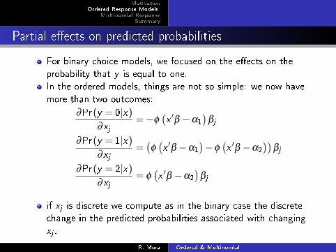
Partial e�ects on predicted probabilities

For binary choice models, we focused on the e�ects on theprobability that y is equal to one.

In the ordered models, things are not so simple: we now havemore than two outcomes:

∂Pr(y = 0|x)

∂xj=−φ

(x ′β −α1

)βj

∂Pr(y = 1|x)

∂xj=(φ(x ′β −α1

)−φ

(x ′β −α2

))βj

∂Pr(y = 2|x)

∂xj= φ

(x ′β −α2

)βj

if xj is discrete we compute as in the binary case the discretechange in the predicted probabilities associated with changingxj .




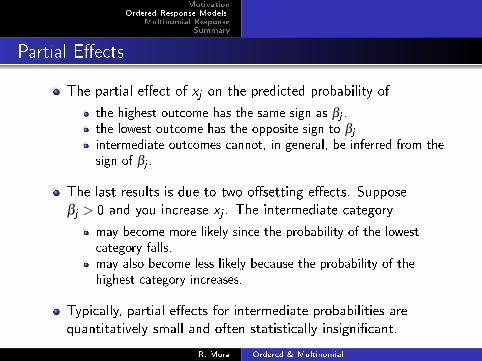
Partial E�ects

The partial e�ect of xj on the predicted probability of

the highest outcome has the same sign as βj .the lowest outcome has the opposite sign to βj

intermediate outcomes cannot, in general, be inferred from thesign of βj .

The last results is due to two o�setting e�ects. Supposeβj > 0 and you increase xj . The intermediate category

may become more likely since the probability of the lowestcategory falls.may also become less likely because the probability of thehighest category increases.

Typically, partial e�ects for intermediate probabilities arequantitatively small and often statistically insigni�cant.




Discussion

How best to interpret results from ordered models?

One option is to look at the estimated β -parameters,emphasizing the underlying latent variable equation with whichwe started.

Another option might be to look at the e�ect on the expectedvalue of the ordered response variable, e.g.

∂E(y |x)

∂xj=

∂Pr(y = 0|x)

∂xj×0+

∂Pr(y = 1|x)

∂xj×1+

∂Pr(y = 2|x)

∂xj×2

This may make a lot of sense if y is a numerical variable, as inthe income variable.

Alternatively, you might just want to report the e�ect on theprobability of observing the ordered categories.




Multinomial Response




The dependent variable is such that

more than two outcomes are possiblethe outcomes cannot be ordered in any natural way.

Again, we could bunch two or more categories and soconstruct a binary outcome variable from the raw data, but indoing so, we throw away potentially interesting information.

OLS is also not a good model in this context.

However, the logit model for binary choice can be extended tomodel more than two outcomes.




Random Utility Model

Assume that there are three transport alternatives: bus, car,train:

Ub = x ′bβb + εb

Uc = x ′cβc + εc

Ut = x ′tβt + εt

where {εb,εc ,εt} are the e�ects on utility unobserved by theeconometrician

If x ′bβb + εb ≥max {x ′cβc + εc ,x′tβt + εt} then y = 0

If x ′cβc + εc >max{x ′bβb + εb,x

′tβt + εt

}then y = 1

If x ′tβt + εt >max {x ′cβc + εc ,x′tβt + εt} then y = 2




Notation

We have two unobserved independent e�ects

ε01 = εb− εc

ε02 = εb− εt

note that ε12 = εc − εt = ε02− ε01

De�ne

x ′bβb− x ′cβc = x ′β01

x ′bβb− x ′tβt = x ′β02




Assumption

{ε01,ε02} ∼ F

where F is symmetric.

Then

Pr(y = 0|x) = Pr(x ′β01 + ε01 ≥ 0,x ′β02 + ε02 ≥ 0|x

)= Pr

(ε01 ≥−

(x ′β01

),ε02 ≥−

(x ′β02

)|x)

Given symmetry,

Pr(y = 0|x) = F(x ′β01,x

′β02

)R. Mora Ordered & Multinomial



Multinomial Logit

We must model the probability that an individual belongs tocategory j conditional to having characteristics x :

Pr(y = j |x)

When vector {εb,εc ,εt} has a extreme value distribution, thenwe have the Multinomial Logit:

Pr(y = 0|x) = 1−Pr(y = 1|x)−Pr(y = 2|x)

Pr(y = 1|x) =exp(x ′β1)

1+ exp(x ′β1) + exp(x ′β2)

Pr(y = 2|x) =exp(x ′β2)

1+ exp(x ′β1) + exp(x ′β2)




The main di�erence compared to the binary logit is that thereare now two parameter vectors, β1 and β2

in the general case with J possible responses, there are J−1parameter vectors.

This makes interpretation of the coe�cients more di�cultthan for binary choice models.




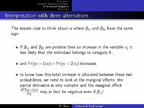
Interpretation with three alternatives

The easiest case to think about is where β1j and β2j have the samesign.

If β1j and β2j are positive then an increase in the variable xj itless likely that the individual belongs to category 0...

and Pr(yi = 1|xi ) +Pr(yi = 2|xi ) increases

to know how this total increase is allocated between these twoprobabilities, we need to look at the marginal e�ects: thepartial derivative is very complex and the marginal e�ect∂Pr(y=1|x)

∂xjmay in fact be negative even if β1j !




Independence of irrelevant alternatives (IIA)

One important limitation of the multinomial logit is that theratio of any two probabilities l and m depends only on theparameter vectors βl and βm and the explanatory variables x

Pr(y = 1|x)

Pr(y = 2|x)=

exp(x ′β1)

exp(x ′β2)

=exp(x ′ (β1−β2)

)The inclusion or exclusion of other categories is irrelevant tothe ratio of the two probabilities.

This behavior is referred to as the �independence of irrelevantalternatives�, and it can lead to counter-intuitive behavior




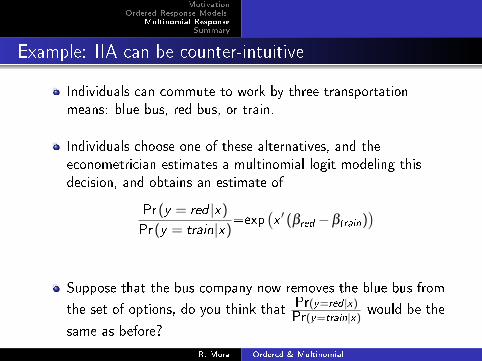
Example: IIA can be counter-intuitive

Individuals can commute to work by three transportationmeans: blue bus, red bus, or train.

Individuals choose one of these alternatives, and theeconometrician estimates a multinomial logit modeling thisdecision, and obtains an estimate of

Pr(y = red |x)

Pr(y = train|x)=exp

(x ′ (βred −βtrain)

)

Suppose that the bus company now removes the blue bus from

the set of options, do you think that Pr(y=red |x)Pr(y=train|x)

would be the

same as before?




Other multinomial models

There are lots of other econometric models that can be usedto model multinomial response models:

multinomial probit,conditional logit,nested logit

They are beyond the scope of the course.




Summary

When the dependent variable has a �nite number of discretevalues, we can extend the probit and logit models

When the dependent variable entails some ordinal information,then we can use ordered probit and logit modelsWhen the dependent variable does not contain any ordinalinformation, we can use multinomial models. One suchexample is the multinomial logit.

These are all nonlinear models, and they can all be estimatedby MLE.


the ordered and multinomial models - uc3m - …ricmora/miccua/materials/s13t31_english...motivation...

Documents