evaluating the effects of morrow's honeysuckle control on

Graduate Theses, Dissertations, and Problem Reports

2011

Evaluating the Effects of Morrow's Honeysuckle Control on Evaluating the Effects of Morrow's Honeysuckle Control on

Vertebrate and Vegetation Assemblages, and Small Mammal Vertebrate and Vegetation Assemblages, and Small Mammal

Foraging Ecology at Fort Necessity National Battlefield Foraging Ecology at Fort Necessity National Battlefield

Charnee Lee Rose West Virginia University

Follow this and additional works at: https://researchrepository.wvu.edu/etd

Recommended Citation Recommended Citation Rose, Charnee Lee, "Evaluating the Effects of Morrow's Honeysuckle Control on Vertebrate and Vegetation Assemblages, and Small Mammal Foraging Ecology at Fort Necessity National Battlefield" (2011). Graduate Theses, Dissertations, and Problem Reports. 3336. https://researchrepository.wvu.edu/etd/3336

This Thesis is protected by copyright and/or related rights. It has been brought to you by the The Research Repository @ WVU with permission from the rights-holder(s). You are free to use this Thesis in any way that is permitted by the copyright and related rights legislation that applies to your use. For other uses you must obtain permission from the rights-holder(s) directly, unless additional rights are indicated by a Creative Commons license in the record and/ or on the work itself. This Thesis has been accepted for inclusion in WVU Graduate Theses, Dissertations, and Problem Reports collection by an authorized administrator of The Research Repository @ WVU. For more information, please contact [email protected].

https://researchrepository.wvu.edu/

https://researchrepository.wvu.edu/

https://researchrepository.wvu.edu/etd

https://researchrepository.wvu.edu/etd?utm_source=researchrepository.wvu.edu%2Fetd%2F3336&utm_medium=PDF&utm_campaign=PDFCoverPages

https://researchrepository.wvu.edu/etd/3336?utm_source=researchrepository.wvu.edu%2Fetd%2F3336&utm_medium=PDF&utm_campaign=PDFCoverPages

mailto:[email protected]

Evaluating the Effects of Morrow’s Honeysuckle Control on Vertebrate and Vegetation

Assemblages, and Small Mammal Foraging Ecology at Fort Necessity National Battlefield

Charneé Lee Rose

Thesis submitted to the

Davis College of Agriculture, Natural Resources and Design

at West Virginia University

in partial fulfillment of the requirements for the degree of

Master of Science

in

Wildlife and Fisheries Resources

James T. Anderson, Ph.D., Major Advisor

George T. Merovich, Ph.D., Committee Member

Petra Bohall Wood, Ph.D., Committee Member

Division of Forestry and Natural Resources

Morgantown, West Virginia

2011

Key Words: American woodcock, bush honeysuckle, diet plasticity, exotic species,

herbicide, herpetofauna, invasive species, microsites, restoration, small mammal,

soft mast, songbird

ABSTRACT

Evaluating the Effects of Morrow’s Honeysuckle Control on Vertebrate and Vegetation

Assemblages, and Small Mammal Foraging Ecology at Fort Necessity National Battlefield

Charneé Lee Rose

Exotic, Japanese bush honeysuckles (Lonicera spp.; Caprifoliaceae) are tied to a variety

of impacts on wildlife and ecosystems. Morrow‟s honeysuckle (Lonicera morrowii) has become

a persistent invader in eastern North America. We organized a restoration initiative at Fort

Necessity National Battlefield (FONE), Pennsylvania, USA from 2004 – 2010. Concurrently, we

studied the consumption of Morrow‟s honeysuckle fruits by small mammals from October –

November 2009 and July – August 2010, and determined habitat variables that affected visitation

rate to foraging stations. Areas of FONE were invaded by Morrow‟s honeysuckle after the land

had been cleared for agriculture, and routine mowing ceased in the mid-1980s. Our restoration

goals were to control honeysuckle and restore native vegetation with a plan to promote both

early-successional habitat and mimic the historical conditions from the mid-1700s. Treatment

and reference sites were established, and treatment sites received a combination of yearly

mowing and broad-spectrum herbicides from October 2006 – August 2010. The vegetation and

vertebrate communities were monitored pre-removal from 2004 – 2006, and throughout the

restoration from 2007 – 2010.

Our control techniques were highly effective at reducing the presence of Morrow‟s

honeysuckle in the treatment area. The percent cover of Morrow‟s honeysuckle declined

dramatically from 2005 – 2010. No direct, short-term adverse impacts on the monitored

vegetation and vertebrate communities occurred. In fact, most species varied as a function of

time over the study, rather than because of the presence or removal of Morrow‟s honeysuckle.

We found that small mammals were better indicators of changes in the vegetation community

than were songbirds. Competitive interactions between small mammals appeared to produce an

indirect negative effect of restoration. Overall, our restoration efforts were successful at

controlling Morrow‟s honeysuckle with minimal impact on the monitored communities.

When compared to native soft mast, Morrow‟s honeysuckle was generally less consumed

by white-footed mice (P. leucopus). Honeysuckle fruits had significantly less protein (0.66%)

and lipids (0.67%) than all natives. Morrow‟s honeysuckle had one of the highest moisture

contents, which was important in the use of its fruits. Despite high moisture content, Morrow‟s

fruits are still lacking key nutrition, likely leading to its overall low consumption. Total energy

always distinguished the highest selected fruits: black cherry (P. serotina) (0.45 kcal), and

common dewberry (R. flagellaris) (0.36). Morrow‟s honeysuckle creates monocultures that

exclude natives, which are the more nutritious and utilized food items. This may force small

mammals to forage longer, or travel further distances with the possibility of increasing their risk

of predation. This result corresponds to our finding that high visitation rate to foraging stations

was negatively associated with shrub coverage in fields. The most common shrub in the field

was Morrow‟s honeysuckle, found to be the closest shrub to 85% of stations. Since honeysuckle

is less nutritious and a lesser-used food item, animals would lose energetic profit if they

continued to feed in areas of honeysuckle, and it likely explains why they do not often forage in

dense honeysuckle areas.

iii

To Donald Edward Rose,

for being the one who gave me my first set of Wildlife Fact File cards,

and for all the penny-candy I could ever eat

– I miss you Grandpa.

iv

ACKNOWLEDGMENTS

I extend my gratitude to Dr. James T. Anderson for not judging a book by its cover, and

giving a sociology major the chance to prove she had what it took to succeed in the life sciences.

Thank you for your patience, for sharing your expertise, and for allowing me to grow into a

young scientist. I thank my other committee members Dr. George T. Merovich and Dr. Petra

Bohall Wood for their advice, support, and for trusting me with valuable field equipment.

I thank the National Park Service and the Environmental Research Center at WVU for providing

funding for this project. Additionally I thank the Natural Resource Specialist at Fort Necessity,

Ms. Connie Ranson, for her guidance, and much needed laughter.

I am indebted to Dr. Phil J. Turk, and Dr. George T. Merovich, for their assistance with

statistical analyses, and for sharing their time and knowledge with me. I thank Dr. James S.

Rentch for taking the time to accompany me during vegetation sampling, and lending his

impressive knowledge to the benefit of the study. Thanks to Tammy Webster and the WVU

Rumen Fermentation lab for performing nutrient content analysis of study fruits. To Paul

Ludrosky for taking the time to help construct the sampling boxes for the foraging study.

I thank Jason P. Love, Jennifer A. Edalgo, and Holly M. McChesney for laying the

groundwork for the Fort Necessity restoration project, and for the years of dedication to

monitoring the biotic community. I thank my fellow graduate student and undergraduates: Jesse

De La Cruz, Wayne Riley, and Frank Klinger for their help with fieldwork and encouragement in

the beginning stages of my project. I thank field tech extraordinaire Jon Holmes for spending the

entire summer trapping small mammals in the pouring rain for nothing more than the experience

and a couple of free meals.

v

To the Rose-Cardoso family, for your love and support of all directions I have taken in

life – especially those that have taken me so far from home – I love you all very much. Thank

you to the wonderful Selego family for their encouragement, kindness, and much appreciated

“life lessons” throughout this endeavor. A final thanks to my partner and fellow WVU graduate

student, Stephen M. Selego, for not only the patience, and unwavering faith but for doubling as

my field technician and making my lengthy field seasons possible.

vi

Table of Contents

ABSTRACT .................................................................................................................................... ii

ACKNOWLEDGMENTS ............................................................................................................. iv

TABLE OF CONTENTS ............................................................................................................... vi

CHAPTER 1. LIST OF FIGURES ..................................................................................................x

CHAPTER 2. LIST OF TABLES .................................................................................................. xi

CHAPTER 2. LIST OF FIGURES ............................................................................................... xii

CHAPTER 3. LIST OF TABLES ................................................................................................ xiv

CHAPTER 3. LIST OF FIGURES ................................................................................................xv

CHAPTER 4. LIST OF TABLES ................................................................................................ xvi

CHAPTER 4. LIST OF FIGURES ............................................................................................. xvii

LIST OF APPENDICES ............................................................................................................ xviii

CHAPTER 1 ....................................................................................................................................1

INTRODUCTION, JUSTIFICATION FOR REMOVAL OF MORROW‟S HONEYSUCKLE

(LONICERA MORROWII), AND PREVIOUS RESEARCH RESULTS FROM FORT

NECESSITY NATIONAL BATTLEFIELD, PENNSYLVANIA ..................................................1

INTRODUCTION ...........................................................................................................................1

JUSTIFICATION ............................................................................................................................3

Restoration Study .................................................................................................................3

Foraging Ecology .................................................................................................................4

STUDY DESCRIPTION ..................................................................................................................5

Study Site .............................................................................................................................5

Objectives ............................................................................................................................6

PREVIOUS RESEARCH RESULTS ..................................................................................................9

Total Non-structural Carbohydrates (TNC) ........................................................................9

Effective Methods for Removing Morrow‟s Honeysuckle ..................................................9

Effects of Morrow‟s Honeysuckle on Invertebrates ............................................................9

Effects of Morrow‟s Honeysuckle on Exotic Earthworms ................................................10

Effects of Morrow‟s Honeysuckle on Prebaiting...............................................................10

Effects of Morrow‟s Honeysuckle on Small Mammal Microhabitat Selection .................10

LITERATURE REVIEW ................................................................................................................11

Restoration Ecology ...........................................................................................................11

Characteristics of Exotic Plants .........................................................................................12

Four Stages of Invasion .....................................................................................................13

Exotic Bush Honeysuckles ................................................................................................15

Wildlife and Exotic Bush Honeysuckles ...........................................................................18

Impacts of Exotic Bush Honeysuckles ..............................................................................19

Management of Exotic Bush Honeysuckles ......................................................................20

Small Mammal Ecosystem Function and Foraging Ecology .............................................21

Previous Small Mammal Food Trials ................................................................................22

Species Detection with Video Monitoring and Fluorescent Powder Tracking..................23

LITERATURE CITED ...................................................................................................................24

vii

CHAPTER 2 ..................................................................................................................................49

RESPONSE OF VERTEBRATE AND VEGETATION COMMUNITIES TO THE CONTROL

OF MORROW‟S HONEYSUCKLE (LONICERA MORROWII) IN SOUTHWESTERN

PENNSYLVANIA .........................................................................................................................49

ABSTRACT ................................................................................................................................49

INTRODUCTION .........................................................................................................................51

MATERIALS AND METHODS ......................................................................................................52

Study Site ...........................................................................................................................52

Restoration Procedures ......................................................................................................53

American Woodcock .........................................................................................................54

Songbirds ...........................................................................................................................54

Small Mammals .................................................................................................................54

Amphibians and Reptiles ...................................................................................................55

Vegetation ..........................................................................................................................56

Data Analysis .....................................................................................................................56

RESULTS ...................................................................................................................................59

Vegetation ..........................................................................................................................59


Songbirds ...........................................................................................................................60

Small Mammals .................................................................................................................61


DISCUSSION ..............................................................................................................................64

Vegetation ..........................................................................................................................64


Songbirds ...........................................................................................................................65

Small Mammals .................................................................................................................66


Conclusions ........................................................................................................................67

IMPLICATIONS FOR PRACTICE ...................................................................................................67

ACKNOWLEDGMENTS ...............................................................................................................68

LITERATURE CITED ...................................................................................................................68

CHAPTER 3 ..................................................................................................................................92

WHITE-FOOTED MOUSE (PEROMYSCUS LEUCOPUS) CONSUMPTION OF INVASIVE

BUSH HONEYSUCKLE FRUITS IN THE NORTHEASTERN UNITED STATES .................92

ABSTRACT ................................................................................................................................92

INTRODUCTION .........................................................................................................................93

MATERIALS AND METHODS ......................................................................................................95

Study Site ...........................................................................................................................95

Foraging Stations ...............................................................................................................96

Fruit Selection ....................................................................................................................96

Consumption Monitoring ...................................................................................................97

Nutrient Composition and Metrics .....................................................................................97

Small Mammal Surveys .....................................................................................................99

viii

Diet Analysis ....................................................................................................................101

Nutrient and Mammal Community Composition Analysis .............................................102

RESULTS .................................................................................................................................103

Small Mammal Community Composition .......................................................................103

Fruit Use...........................................................................................................................104

Fruit Species Characteristics ............................................................................................105

DISCUSSION ............................................................................................................................106

Characteristics Affecting Use ..........................................................................................106

Temporal Variation in Characteristics .............................................................................107

Characteristics with Low Influence on Use .....................................................................107

Additional Factors Affecting Foraging ............................................................................108

Morrow‟s Honeysuckle Fruit Characteristics ..................................................................109

Dominant Species and Monitoring Techniques ...............................................................110

Nutrition and Energy Expenditure ...................................................................................111

ACKNOWLEDGMENTS .............................................................................................................111

LITERATURE CITED .................................................................................................................112

CHAPTER 4 ................................................................................................................................127

HABITAT CHARACTERISTICS THAT AFFECT WHITE-FOOTED MOUSE

(PEROMYSCUS LEUCOPUS) VISITATION RATE TO FORAGING STATIONS .................127

ABSTRACT ..............................................................................................................................127

INTRODUCTION .......................................................................................................................128

MATERIALS AND METHODS ....................................................................................................130

Study Site .........................................................................................................................130

Visitation Rate .................................................................................................................131

Habitat Surveys ................................................................................................................132

Data Analysis ...................................................................................................................133

RESULTS .................................................................................................................................137

DISCUSSION ............................................................................................................................138

Seasonal, Influential Environmental Variables ................................................................138

Shrub Species Impact on Visitation .................................................................................140

Spatial Influence on Visitation.........................................................................................141

Conclusions ......................................................................................................................142

ACKNOWLEDGMENTS .............................................................................................................143


CHAPTER 5 ................................................................................................................................163

REVIEW OF CONCLUSIONS AND MANAGEMENT IMPLICATIONS FOR FORT

NECESSITY NATIONAL BATTLEFIELD, FARMINGTON, PENNSYLVANIA, IN

RELATION TO THE CONTROL OF MORROW‟S HONEYSUCKLE (LONICERA

MORROWII) ................................................................................................................................163

INTRODUCTION .......................................................................................................................163

OBJECTIVES ............................................................................................................................164

RESULTS .................................................................................................................................166

ix

Impacts of Honeysuckle and Restoration Procedures ......................................................166

Vegetation ..................................................................................................................166

American Woodcock ..................................................................................................167

Songbirds ...................................................................................................................168

Small Mammals ..........................................................................................................169

Herpetofauna .............................................................................................................170

Small Mammal Foraging Study .......................................................................................170

Fruit Use ....................................................................................................................170

Effects on White-footed Mice .....................................................................................172

Small Mammal Habitat Use .............................................................................................172

Variables Affecting Visitation ....................................................................................172

Shrub Species Impact .................................................................................................173

Spatial and Seasonal Differences ..............................................................................174

MANAGEMENT IMPLICATIONS ................................................................................................175


x

CHAPTER 1. LIST OF FIGURES ................................................................................................41

Figure 1. Fort Necessity National Battlefield lies in Fayette County, Pennsylvania, USA. ..........41

Figure 2. Project study sites are located within the 390 ha boundary of Fort Necessity National

Battlefield, Pennsylvania, USA, from 2004-2010. ........................................................................42

Figure 3. The study site is adjacent to the replica of Fort Necessity, at Fort Necessity National

Battlefield, Pennsylvania, USA... ..................................................................................................43

Figure 4. Historical recreation of Fort Necessity at Fort Necessity National Battlefield,

Pennsylvania, USA. The original was constructed by George Washington and his troops at the

onset of the French and Indian War. ..............................................................................................43

Figure 5. The study site was characterized by a monoculture of Morrow‟s honeysuckle (Lonicera

morrowii) before treatment in 2003, at Fort Necessity National Battlefield, Pennsylvania,

USA…............................................................................................................................................44

Figure 6. Previous graduate researcher, Jason P. Love, applying herbicide treatment to selected

honeysuckle plots at Fort Necessity National Battlefield, Pennsylvania, USA, in 2005...............44

Figure 7. September 2007 application of Arsenal® (imidazole) to the treatment area via all-

terrain vehicle, at Fort Necessity National Battlefield, Pennsylvania, USA .................................45

Figure 8. Foraging ecology study box locations throughout the 390 ha boundary of Fort

Necessity National Battlefield, Pennsylvania, USA, 2009-2010 ...................................................46

Figure 9. The flowers of Morrow‟s honeysuckle (Lonicera morrowii) bloom from May-June....47

Figure 10. Morrow‟s honeysuckle (Lonicera morrowii) begins fruiting in June and can carry its

paired red fruits through autumn....................................................................................................47

Figure 11. The branch architecture of Morrow‟s honeysuckle (Lonicera morrowii), and absence

of thorns, leaves nesting birds open to predation; although difficult for human navigation,

predators like raccoons can easily move through the less dense understory of the shrub. ............48

xi

CHAPTER 2. LIST OF TABLES ..................................................................................................75

Table 1. Vector relations to nonmetric multi-dimensional scaling (NMDS) ordination of biotic

communities at Fort Necessity National Battlefield, Pennsylvania, USA, 2005, 2008, and 2010.

A significance of 0.1 is denoted by (Ο), 0.05 by (*), 0.01 by (**), and 0.001 by (***) ................75

Table 2. Impact of restoration removal procedures on various biotic communities sampled during

the restoration process at Fort Necessity National Battlefield, Pennsylvania, USA from 2004-

2010................................................................................................................................................77

xii

CHAPTER 2. LIST OF FIGURES ................................................................................................78

Figure 1. The Fort Necessity National Battlefield, Pennsylvania, USA, study site was

characterized by a dense monoculture of Morrow‟s honeysuckle in 2004 before treatment ........78

Figure 2. Project study sites were located within the 390 ha boundary of Fort Necessity National

Battlefield, Pennsylvania, USA, from 2004-2010 .........................................................................79

Figure 3. Timeline of major restoration procedures from October 2006 – August 2010 at Fort

Necessity National Battlefield, Pennsylvania, USA ......................................................................80

Figure 4. The post-removal treatment site at Fort Necessity National Battlefield, Pennsylvania,

USA, after September 2009 planting of native shrubs ..................................................................80

Figure 5. Mean (± SE) change in percent cover of Morrow‟s honeysuckle and native shrubs and

shrub species in reference and treatment plots at Fort Necessity National Battlefield,

Pennsylvania, USA, during pre-removal (2005), and post-removal (2008, 2010). Different

lowercase letters indicate differences (p < 0.05) within plot types across years. Different capital

letters indicate differences (p < 0.05) within a year, between plot types. Different capital letters

below years indicate differences (p < 0.05) between years ...........................................................81

Figure 6. Mean (± SE) change in vegetation richness, coefficient of conservatism and floristic

quality in reference and treatment plots at Fort Necessity National Battlefield, Pennsylvania,

USA, during pre-removal (2005), and post-removal (2008, 2010). Different capital letters below

years indicate differences (p < 0.05) between years ......................................................................82

Figure 7. Mean (± SE) change in vegetation evenness in reference and treatment plots at Fort

Necessity National Battlefield, Pennsylvania, USA, during pre-removal (2005), and post-

removal (2008, 2010). Different lowercase letters indicate differences (p < 0.05) within plot

types across years. Different capital letters indicate differences (p < 0.05) within a year, between

plot types ........................................................................................................................................83

Figure 8: Nonmetric multidimensional scaling (NMDS) ordination of vegetation surveys (Bray–

Curtis matrix) conducted at Fort Necessity National Battlefield, Pennsylvania, USA, in 3

dimensions showing sites labeled by type (T = Treatment, R = Reference), years (2005, 2008,

2010), habitat vectors, and weighted means positions of selected species that have strong

correlation to the ordination. Pre-removal surveys were in year 2005, post-removal surveys were

in years 2008 and 2010. Stress = 7.0 in the 3-dimensional solution. Vectors are significant at p =

0.05. Exotics stands for the average richness of exotic species .....................................................84

Figure 9. Mean (± SE) change in American woodcock hear calling in reference and treatment

plots at Fort Necessity National Battlefield, Pennsylvania, USA, during pre-removal (2004 –

2006), and post-removal (2007 – 2010). Different lowercase letters indicate differences (p <

0.05) within plot types across years. Different capital letters indicate differences (p < 0.05)

within a year, between plot types ...................................................................................................85

xiii

Figure 10. Mean (± SE) change in songbird diversity and richness in reference and treatment

plots at Fort Necessity National Battlefield, Pennsylvania, USA, during pre-removal (2004), and

post-removal (2008, 2010). Different capital letters below years indicate differences (p < 0.05)

between years .................................................................................................................................86

Figure 11. Nonmetric multidimensional scaling (NMDS) ordination of songbird point count

surveys (Bray–Curtis matrix) from Fort Necessity National Battlefield, Pennsylvania, USA, in 3

dimensions showing sites labeled by type (T = Treatment, R = Reference), year (2004, 2008,




0.05. FQI is code of the plant floristic quality index, H is for songbird species diversity, and S is

for songbird species richness .........................................................................................................87

Figure 12. Mean (± SE) change in total relative abundance, meadow jumping mouse, and white-

footed mouse densities, in reference and treatment plots at Fort Necessity National Battlefield,

Pennsylvania, USA, during pre-removal (2004 – 2006), and post-removal (2007 – 2010).

Different lowercase letters indicate differences (p < 0.05) within plot types across years.

Different capital letters indicate differences (p < 0.05) within a year, between plot types.

Different capital letters below years indicate differences (p < 0.05) between years .....................88

Figure 13. Mean (± SE) change in meadow vole densities from Sherman and pitfall traps, in

reference and treatment plots at Fort Necessity National Battlefield, Pennsylvania, USA, during

pre-removal (2004 – 2006), and post-removal (2007 – 2010). Different lowercase letters indicate

differences (p < 0.05) within plot types across years. Different capital letters indicate differences

(p < 0.05) within a year, between plot types. Different capital letters below years indicate

differences (p < 0.05) between years .............................................................................................89

Figure 14. Nonmetric multidimensional scaling (NMDS) ordination of small mammal Sherman

trapping (Bray–Curtis matrix) from Fort Necessity National Battlefield, Pennsylvania, USA, in 3




in years 2008 and 2010.Stress = 2.7 in the 3-dimensional solution. Vectors are significant at p ≤

0.05. Code is as follows: CPUE = captures/100 trap nights, C = plant coefficient of conservatism,

H = small mammal species diversity, J = small mammal species evenness ..................................90

Figure 15. Nonmetric multidimensional scaling (NMDS) ordination of small mammal pitfall

arrays (Bray–Curtis matrix) from Fort Necessity National Battlefield, Pennsylvania, USA, in 3




in years 2008 and 2010. Stress = 6.2 in the 3-dimensional solution. All vectors shown are

significant at p = 0.05. Code is as follows: FQI = plant floristic quality index .............................91

xiv

CHAPTER 3. LIST OF TABLES ................................................................................................120

Table 1. Small mammal species identified, time observed, and fruit consumed during camera

trials at Fort Necessity National Battlefield, Pennsylvania, USA, October 2009 – August 2010.

The standard error (SE) for time is reported in minutes. Successful nights were determined for

each cover type out of 20 trials. Success was defined as a night when at least one small mammal

was observed ................................................................................................................................120

Table 2. Captures per 100 trap nights (CPUE) by small mammal species and total at Fort

Necessity National Battlefield, Pennsylvania, USA, during October 2009 – August 2010,

using Sherman live traps. Means in a row with different uppercase letters are significantly

different at P < 0.05, based on Tukey‟s multiple comparisons. Only CPUE, white-footed mouse

and meadow vole abundances were tested statistically due to low number of captures for other

species ..........................................................................................................................................121

Table 3. Simplified ranking matrix of foraging boxes based on comparing foraging categories

during each round at Fort Necessity National Battlefield, Pennsylvania, USA, from October 2009

– August 2010. Matrices of log-ratio differences were constructed for each box based on pooled

observations. A species in a row was used significantly (P < 0.05) more (+ + +) or less

(- - -) compared to the column headings. Single signs (+ or -) indicate a numerical, but not

significant, difference. The number of positive values correspond to the rank for each foraging

category, with the highest ranked item being the most consumed ..............................................122

Table 4. Mean (± SE) number of fruits consumed per box by cover type and overall average at

Fort Necessity National Battlefield, Pennsylvania, USA. Original data are provided for ease of

interpretation, while significances (P < 0.05) are based on log-ratio differences in statistical tests.

Different uppercase letters in the column “Overall” indicate differences among species in a

round. Different uppercase letters behind means of native species under a cover type represent a

significant change in the magnitude of use (i.e., the difference between the mean numbers of

fruits consumed) for a native species compared to honeysuckle across cover types within a

round. Different lower case letters indicate a significant difference in consumption of a fruit

across cover types within a round. Differences are based on Tukey‟s multiple comparisons .....123

Table 5. Nutrient composition and physical characteristics of all fruit species used during

foraging trials from October 2009 – August 2010 at Fort Necessity National Battlefield,

Pennsylvania, USA. Means in a column with different uppercase letters are significantly

different at P < 0.05, based on Tukey‟s multiple comparisons, except for handling time, which is

significant at P < 0.002, based on Bonferroni corrected Mann – Whitney U tests .....................124

xv

CHAPTER 3. LIST OF FIGURES ..............................................................................................125

Figure 1. Foraging boxes that were placed throughout Fort Necessity National Battlefield,

Pennsylvania, USA, from October 2009 – August 2010 .............................................................125

Figure 2. Foraging box locations throughout the 390 ha boundary of Fort Necessity National

Battlefield, Pennsylvania, USA, October 2009 – August 2010, with emphasis on the 100 m

separation between boxes ............................................................................................................126

xvi

CHAPTER 4. LIST OF TABLES ................................................................................................152

Table 1. Mean (± SE) for the environmental variables found in the best models for predicting

visitation rate to foraging stations at Fort Necessity National Battlefield, Pennsylvania, USA in

October – November 2009 (Fall) and July – August 2010 (Summer). All values were averaged

over 20 stations within each cover type (total N = 60) ................................................................152

Table 2. A priori models for visitation rate to foraging stations in edges, fields, and forests at Fort

Necessity National Battlefield, Pennsylvania, USA in October – November 2009 (Fall) and July

– August 2010 (Summer) at 100 m2 and 400 m

2 scales. The best model is chosen by Akaike‟s

Information Criterion for small sample sizes (AICc), with small values indicating a better model

fit. Model variables include: percent plot coverage of living plants (GN), grass (GS), forb (FB),

fern (FN), moss (MS), shrub (SB), tree (TE), leaf (LF), log (LG), rock (RK), road (RD) and dead

plants (DPM); visual obscurity measurements (tallest sight, TS and first sight, FS), canopy cover

(CC); ground slope (SL), soil moisture (SM); closest shrub (SD) and tree (TD) distances to box,

closest shrub stems (SN) and volume (SV); closest tree height (TH), diameter at breast height

(DBH), and crown width (CW) ...................................................................................................154

Table 3. Parameter estimates (± SE) for models with substantial support for predicting visitation

rate at edge, field and forest foraging stations at Fort Necessity National Battlefield,

Pennsylvania, USA in October – November 2009 (Fall) and July – August 2010 (Summer) at

100 m2 and 400 m

2 scales. Model variables included: percent plot coverage of grass (GS), forb

(FB), fern (FN), shrub (SB), tree (TE), leaf (LF), log (LG), rock (RK); visual obscurity

measurements (tallest sight, TS and first sight, FS), canopy cover (CC); soil moisture (SM) and

closest tree (TD) distance to box .................................................................................................160

xvii

CHAPTER 4. LIST OF FIGURES ..............................................................................................162

Figure 1. Foraging station locations throughout the 390 ha boundary of Fort Necessity National

Battlefield, Pennsylvania, USA, from 2009-2010 with emphasis on the habitat survey spatial

scales ............................................................................................................................................162

xviii

LIST OF APPENDICES ..............................................................................................................182

CHAPTER 2. APPENDICES ......................................................................................................182

Appendix Ia: Location of the Outer Meadow and Inner Meadow trails in the treatment and

reference plots at Fort Necessity National Battlefield, Pennsylvania, USA. American woodcock

were often observed using these specific mowed paths in the park from 2004-2010 .................182

Appendix IIa. Location of reference and treatment areas including corresponding small mammal

Sherman trapping grids, vegetation survey points, bird point count locations, and pitfall trapping

arrays at Fort Necessity National Battlefield, Pennsylvania, USA, 2004-2010 ..........................183

Appendix IIIa. Each pitfall array consisted of four 20-liter buckets placed in a triad and

connected with a 3-m long, 50-cm high silt fence. Six pitfall trap arrays, and 36 cover boards

were placed throughout the study area at Fort Necessity National Battlefield, Pennsylvania,

USA, 2004-2010 ..........................................................................................................................184

Appendix IVa. Biotic community variables with non-significant F-tests, based on data collected

from Fort Necessity National Battlefield, Pennsylvania, USA, 2004-2010 ................................185

Appendix Va. Plant species identified at 12 random sampling points in reference (R) and

treatment (T) plots at Fort Necessity National Battlefield, Pennsylvania, USA, in 2005, 2008, and

2010. Species in bold are exotic. Coefficient of conservatism (C) is given for each species ......186

Appendix VIa. The most common shrub species identified, based on percent plot coverage,

across Fort Necessity National Battlefield, Pennsylvania, USA, from 2005, 2008, and 2010

averaged. Any species with a total cover of 5% and greater were included in the table. Species in

bold are exotic ..............................................................................................................................190

Appendix VIIa. Mean ( ) and SE of floristic metrics measured at reference and treatment plots at

Fort Necessity National Battlefield, Pennsylvania, USA, during 2005, 2008, and 2010. *Post-

removal surveys took place following removal procedures ........................................................191

Appendix VIIIa. The most common herbaceous species identified, based on percent plot

coverage, across Fort Necessity National Battlefield, Pennsylvania, USA, from 2005, 2008, and

2010 averaged. Any species with a total cover of 5% and greater were included in the table.

Species in bold are exotic ............................................................................................................193

Appendix IXa: Overall mean ( ) and SE of male American woodcock for the overall reference

and treatment areas at Fort Necessity National Battlefield, Pennsylvania, USA. We performed

singing ground surveys from 2004 throughout 2010 during the winter and spring breeding

months (February – May). *Post-removal surveys took place following the implementation of

management procedures designed to remove Morrow‟s honeysuckle ........................................194

Appendix Xa: Mean ( ) and SE of male American woodcock for individual reference and

treatment plots at Fort Necessity National Battlefield. We performed singing ground surveys

xix

from 2004 throughout 2010 during the winter and spring breeding months (February – May).

*Post-removal surveys took place following the implementation of management procedures

designed to remove Morrow‟s honeysuckle ................................................................................195

Appendix XIa: Mapped locations of male American woodcock heard calling in reference and

treatment plots at Fort Necessity National Battlefield, Pennsylvania, USA, by survey day, in year

2004. Year 2004 represents a pre-removal year. Corresponding descriptive statistics are given:

total number of males heard calling/year, mean number of males/survey day, and highest number

of males/survey day .....................................................................................................................196

Appendix XIIa: Mapped locations of male American woodcock heard calling in reference and





Appendix XIIIa: Mapped locations of male American woodcock heard calling in reference and





Appendix XIVa: Mapped locations of male American woodcock heard calling in reference and


2007. Year 2007 represents a post-removal year. Corresponding descriptive statistics are given:



Appendix XVa: Mapped locations of male American woodcock heard calling in reference and





Appendix XVIa: Mapped locations of male American woodcock heard calling in reference and





Appendix XVIIa: Mapped locations of male American woodcock heard calling in reference and





xx

Appendix XVIIIa: Species of songbirds and their associated habitat guilds observed at Fort

Necessity National Battlefield, Pennsylvania, USA, during 2004, 2008, and 2010 point counts

surveys .........................................................................................................................................203

Appendix XIXa: Total songbird species observations during point count surveys at Fort

Necessity National Battlefield, Pennsylvania, USA, during 2004, 2008, and 2010. Observations

are categorized based on plot type and timing of restoration (Pre-T, Post-T, Pre-R, Post-R). Code

is as follows: T=treatment, R=Reference, Pre = 2004, Post = 2008, 2010 ..................................205

Appendix XXa: Mean ( ) and SE of songbird metrics measured at reference and treatment point

count locations at Fort Necessity National Battlefield, Pennsylvania, USA. We performed point

count surveys during the 2004, 2008, and 2010 breeding period. Numbers of observations of the

2 most common species captured are listed using the following species codes: Eastern towhee

(EATO), and Field sparrow (FISP). *Post removal surveys took place following the

implementation of management procedures designed to remove Morrow‟s honeysuckle ..........206

Appendix XXIa: Total small mammal species captures during Sherman trapping at Fort

Necessity National Battlefield, Pennsylvania, USA, from 2004 – 2010. Observations are

categorized based on plot type and timing of restoration (Pre-T, Post-T, Pre-R, Post-R). Code is

as follows: T=treatment, R=Reference, Pre = 2005, Post = 2008, 2010 .....................................207

Appendix XXIIa: List of mammal species and their associated observation method at Fort

Necessity National Battlefield, Pennsylvania, USA, 2004 – 2010 ..............................................208

Appendix XXIIIa: Mean ( ) and SE of small mammal relative abundance (No. of captures/100

trap nights) and metrics measured at reference and treatment trapping grids at Fort Necessity

National Battlefield, Pennsylvania, USA. We performed Sherman live trapping from 2004

through 2010 during the summer season from May-August. *Post-removal surveys took place

following the implementation of management procedures designed to remove Morrow‟s

honeysuckle..................................................................................................................................209

Appendix XXIVa: Total small mammal species captures during pitfall arrays at Fort Necessity

National Battlefield, Pennsylvania, USA, from 2004 – 2010. Observations are categorized based

on plot type and timing of restoration (Pre-T, Post-T, Pre-R, Post-R). Code is as follows:

T=treatment, R=Reference, Pre = 2005, Post = 2008, 2010 ........................................................213

Appendix XXVa: Mean ( ) and SE of small mammal relative abundance (No. of captures/100

trap nights) and metrics measured at reference and treatment pitfall arrays at Fort Necessity

National Battlefield, Pennsylvania, USA. We trapped using the pitfall arrays from 2004 through

2010 during the summer season from May-August. *Post-removal surveys took place following

the implementation of management procedures designed to remove Morrow‟s honeysuckle ....214

Appendix XXVIa: List of Amphibians and Reptiles species and their associated observation

method at Fort Necessity National Battlefield, Pennsylvania, USA, from 2004 – 2010 .............217

xxi

Appendix XXVIIa: Total herpetofauna species captures during pitfall arrays at Fort Necessity

National Battlefield from 2004 – 2010. Observations are categorized based on plot type and

timing of restoration (Pre-T, Post-T, Pre-R, Post-R). Code is as follows: T=treatment,

R=Reference, Pre = 2005, Post = 2008, 2010 ..............................................................................218

Appendix XXVIIIa: Total herpetofauna species captures during cover board flips at Fort

Necessity National Battlefield from 2004 – 2010. Observations are categorized based on plot

type and timing of restoration (Pre-T, Post-T, Pre-R, Post-R). T=treatment, R=Reference, Pre =

2005, Post = 2008, 2010 ..............................................................................................................219

Appendix XXIXa: Mean ( ) and SE of herpetofauna relative abundance (No. of captures/100

trap nights) at reference and treatment pitfall arrays at Fort Necessity National Battlefield,

Pennsylvania, USA. We trapped using the pitfall arrays from 2004 through 2010 during the

summer season from May-August. *Post-removal surveys took place following the


Appendix XXXa: Mean ( ) and SE of herpetofauna relative abundance (No. of captures/100 trap

nights) at reference and treatment cover board arrays at Fort Necessity National Battlefield,

Pennsylvania, USA. We trapped using the cover board arrays from 2004 through 2010 during the

summer season from May-August. *Post-removal surveys took place following the



Appendix Ib. Fruit species located during two study rounds at Fort Necessity National

Battlefield, Pennsylvania, USA, from October 2009 – August 2010. Study species were chosen

using a random number generator. When species could not be located in sufficient quantities,

another species was chosen at random to replace it .....................................................................224


Appendix Ic. Values for the environmental variables measured at each foraging station at Fort

Necessity National Battlefield, Pennsylvania, USA, in October – November 2009 (fall) and July

– August 2010 (summer). All values were averaged over 20 stations within each cover type (total

N=60). Averaged values (Mean), standard errors (SE), minimum values (Min) and maximum

values (Max) are reported ............................................................................................................225

1

CHAPTER 1

REVIEW ARTICLE

Introduction, Justification for Removal of Morrow‟s Honeysuckle (Lonicera morrowii), and

Previous Research Results from Fort Necessity National Battlefield, Farmington, Pennsylvania

Charneé Lee Rose1,2

Introduction

The economic damages associated with invasive species and their control was estimated

to be about $138 billion per year in the U.S. (Pimentel 2002). Global travel and international

trade have become pathways to accelerated invasion (Mack & Erneberg 2002), increasing

monetary losses. In the biological context, ~40% of endangered species in the United States are

at risk due to competition or predation by non-indigenous species (Wilcove et al. 1998).

Although both animal and plant exotics contribute to the damages described above, exotic plants

alone can spread prolifically (Manchester & Bullock 2000), deteriorate ecosystem services

(Gordon 1998; Ehrenfield 2003), and negatively impact global economies (Naylor 2000;

Zavaleta 2000).

Northeastern and mid-western portions of the United States have been invaded by

aggressive Eurasian bush honeysuckles. Exotic honeysuckles were introduced to the U.S.

through the ornamental industry in the mid-1700s, including Amur honeysuckle (Lonicera

maackii), Morrow‟s honeysuckle (Lonicera morrowii), and Tartarian honeysuckle (Lonicera

tatarica) (Rehder 1940; Luken & Thieret 1995). Bush honeysuckles have a strong tolerance for a

-----------------------------

1 Division of Forestry and Natural Resources, Wildlife and Fisheries Resources Program,

West Virginia University, PO Box 6125, Percival Hall, Morgantown, WV 26506, U.S.A. 2

Address correspondence to C. L. Rose, email: [email protected]

This chapter written in the style of Restoration Ecology

2

broad range of soil moisture, soil types, light regimes and cover types. They grow in riparian

areas, early successional habitat (McClain & Anderson 1990), forest interiors (Woods 1993),

edges, and corridors. The shrubs also occupy areas of disturbed land including roadsides,

railroads (Barnes & Cottam 1974), and abandoned agricultural land (Hauser 1966). Humans

furthered the range of these shrubs by using them in mine reclamations (Wade 1985), shelterbelts

(Herman & Davidson 1997), and for wildlife resources (Mulvihill et al. 1992; VanDruff et al.

1996). A variety of honeysuckle species were widely distributed across the northeastern United

States by the early 1900s (Rehder 1903).

Large areas of Fort Necessity National Battlefield (FONE) were invaded by one of these

invasive bush honeysuckles, Morrow‟s honeysuckle (Lonicera morrowii) (National Park Service

1991). According to the General Management Plan for FONE, the park will be managed to: 1)

prevent damage by exotic species, 2) protect rare, threatened, or endangered species, and 3)

reestablish historical vegetative conditions (National Park Service 1991). An additional plan was

developed to control Morrow‟s honeysuckle by restoring a portion of the study site to a mature

hardwood forest, and to manage the remaining area as early successional habitat for a declining

game bird, the American woodcock (Scolopax minor). To determine the impacts of both

Morrow‟s honeysuckle cover and control procedures we performed pre-treatment and post-

treatment surveys of American woodcock, songbird, small mammal, herpetofauna, and

vegetation communities. Also, we conducted a secondary study examining the effects of

Morrow‟s honeysuckle on small mammal foraging ecology, while concurrently examining

habitat affinities in 2009 and 2010.

3

Justification

Restoration

The support for the restoration research conducted at Fort Necessity National Battlefield

comes from the need to study invasive species to develop methods for both efficient removal and

subsequent reestablishment of natural ecosystems (Hartman & McCarthy 2004). Understanding

trends in the invasion process, as well as the impact of control and management activities, is

necessary to manage exotics (Hunter & Mattice 2002). Studies measuring the effects of exotic

plant species on native communities are lacking (Tickner et al. 2001; Hejda et al. 2009). Previous

to the implementation of this research project, no studies were found that examined the effect of

Morrow‟s honeysuckle removal on native vegetation. Likewise, there is no comprehensive

project known to assess the response of vertebrate populations (songbirds, small mammals,

amphibians, and reptiles) to the removal of invasive Morrow‟s honeysuckle. Due to the

aggressiveness of Morrow‟s honeysuckle, control is difficult; however, the removal of this exotic

at local sites is a critical step in restoring the habitat and developing management practices

(Hartman & McCarthy 2004). Small-scale removal of Morrow‟s honeysuckle is important in

order to continue removal on a “site-by-site basis” across the landscape (Wiens et al. 1993;

Hartman & McCarthy 2004).

Additionally, we placed special emphasis on American woodcock, as it is a popular game

bird with declining populations in portions of the United States (i.e., eastern and Midwestern).

This species uses wetlands and early successional areas as nesting and foraging habitat; however,

both are currently at risk due to habitat destruction and afforestation (Dwyer et al. 1983; Sauer &

Bortner 1991). Long-term declines (1967-2010) have taken place in woodcock populations

across the eastern and central United States (Cooper & Parker 2010). Since populations of this

popular game bird are known to be declining (Brown et al. 2004; Kelley 2004; Cooper & Parker

4

2010), it has been listed by the U.S. Fish and Wildlife Service as a Game Bird Below Desired

Condition (U.S. Fish and Wildlife Service 2004). Also, it is listed on the Audubon Watchlist as a

species that is in slow decline and of national conservation concern (National Audubon Society

2010). Due to this species‟ importance, as both a consumptive and non-consumptive species, it

was critical to assess the potential habitat quality for woodock at Fort Necessity to create an area

of sustainable habitat.

Small Mammal Foraging Ecology

The research conducted by Edalgo et al. (2009) highlights the need for additional studies

to be conducted that further investigate how Morrow‟s honeysuckle alters small mammal

ecology. This paper expressed the need for a study that determines if white-footed mice, as well

as other small mammals, readily consume the fruit and seeds of bush honeysuckle. Additionally,

a number of other studies suggest that exotic plants, especially Lonicera spp., have the potential

to alter small mammal behaviors (Witmer 1996; Williams 1999). Bush honeysuckles outcompete

and greatly reduce native vegetation (Batcher & Stiles 2000); therefore, it is likely that bush

honeysuckles affect the food available to the small mammal species that serve vital roles in the

ecosystem (Bellows et al. 2001).

As the spread of bush honeysuckle continues throughout the United States, it is important

to study the extent to which small mammals incorporate Lonicera into their diets, and determine

if they influence the population dynamics of exotic bush honeysuckle. This information is

necessary as small mammal seed consumption has been shown to influence the spread of native

plant species (Ostfeld et al. 1997); if the same is true for exotics, small mammals could

experience a decrease in species diversity (Horncastle et al. 2004).

For foraging studies to successfully examine preference, it is necessary to understand the

habitat characteristics and microsites that small mammals show fidelity towards. Not only is it

5

important to determine these characteristics, but it is equally as valuable to understand how these

change over various habitats and seasons. Knowledge of selected habitat characteristics and

seasonal variability can increase a study‟s likelihood of detecting species and capturing small

mammal food preference, while increasing the statistical power of their analyses.

Study Description

Study Site

We conducted both the primary (restoration response) and secondary (foraging behavior;

habitat modeling) studies at Fort Necessity National Battlefield. The National Park Service

established Fort Necessity National Battlefield, located in Fayette County in southwestern

Pennsylvania, U.S.A, in 1933 (Fig. 1) (39º48‟43” N, 84º 41‟50” W). The historical park is

approximately 390 ha in size (Fig. 2). Elevations throughout the park range from 535 – 710 m.

The average annual temperature at Fort Necessity is 9º C, the mean winter temperature is -3º C,

and the mean summer temperature is 22º C. The average precipitation level is 119 cm (National

Park Service 1991). Brinkerton and Armagh silt loams characterize the soils; they are moderate

to well drained, medium-textured, and moderately deep (Kopas 1973).

The restoration project sites are located west of an historical replication of Fort Necessity.

The original was built by George Washington and his troops in 1754 at the onset of the French

and Indian War (Figs. 3 & 4). During the mid-1700s, the hillside was predominantly an oak-

hardwood forest. Core pollen samples taken from the site showed that oaks (Quercus spp.), red

maple (Acer rubrum), hickories (Carya spp.), American beech (Fagus grandifolia) and birch

(Betula spp.) comprised the forest (Kelso 1994). After the war, the land was cleared for pasture

use prior to the establishment of the park in 1933 (National Park Service 1991). Until the mid-

1980s, the pasture was maintained by mowing. When the agricultural practices ended, the land

6

was passively managed and allowed to follow natural succession (Love & Anderson 2009).

However, a dense cover of Morrow‟s honeysuckle (Fig. 5) (Love & Anderson 2009) established

and dominated the study area until restoration procedures, which involved a combination of

mowing and herbicide (Figs. 6 & 7), started in 2007.

The foraging ecology study sites are widely distributed across cover types throughout

Fort Necessity that are inhabited by Morrow‟s honeysuckle (Fig. 8). We chose study locations in

three available types: field, edge, and forested areas. Although forested locations in the park

contain less Morrow‟s honeysuckle, we believed it was important to include this cover type in

the study as bush honeysuckles are known to be shade tolerant and hybrids are often found in

forest interiors (Woods 1993).

Objectives

The overall objectives of this project were to:

1) assess the best time (according to shrub‟s phenological stage) to apply herbicide or

mechanically remove Morrow‟s honeysuckle;

2) determine the most effective and cost-efficient method to control Morrow‟s honeysuckle;

3) determine the species composition of shrub and herbaceous communities prior to, and

following restoration procedures;

4) determine the relative abundance and location of American woodcock (Scolopax minor)

prior to, and following restoration procedures;

5) assess the relative abundance and location of earthworms, the woodcock‟s major prey

sources, within the study area;

6) assess the effects of Morrow‟s honeysuckle on the diversity and biomass of insects;

7) determine the relative abundance and richness of amphibians and reptiles within the study

area prior to, and following restoration procedures;

8) determine changes in relative abundance and richness of songbirds in response to

management activities;

7

9) assess the effects of Morrow‟s honeysuckle on songbird fitness level (fat class and body

mass index), and nest success;

10) determine the effects of Morrow‟s honeysuckle on songbird territory size and density;

11) determine the relative abundance and richness of small mammals within the study area

prior to and following restoration procedures;

12) assess the effectiveness of prebaiting Sherman traps within the study area dominated by

Morrow‟s honeysuckle;

13) assess the effects of Morrow‟s honeysuckle on microhabitat selection of small mammals;

14) assess the species of small mammals that actively consume Morrow‟s honeysuckle fruits;

15) investigate if small mammals use Morrow‟s honeysuckle in their diet in the same

quantities as native soft mast fruits;

16) determine if the magnitude of Morrow‟s fruit consumption remains consistent across

cover types, and throughout seasonal changes of Morrow‟s fruiting period;

17) assess the habitat characteristics that contribute to high small mammal visitation rate to

foraging stations across cover types, seasons, and spatial scales; and

18) develop a set of management options for the removal of Morrow‟s honeysuckle and the

consequences each of these options may have on flora and fauna within the study area.

My research focuses on objectives: 3, 4, 7, 8, 11, 14, 15, 16, and 17. Based on these objectives,

and subsequent literature reviews, the following hypotheses were tested:

3) determine the species composition of shrub and herbaceous communities prior to, and

following restoration procedures;

H0: There is no difference in species composition of shrub and herbaceous species

in the study plots prior to, and following restoration.

Ha: There is a difference in composition of shrub and herbaceous species, with

restoration plots showing higher species diversity.

4) determine the relative abundance and location of American woodcock (Scolopax minor)

prior to, and following restoration techniques;

H0: American woodcock will use the study area indiscriminately prior to and

following restoration.

Ha: American woodcock abundance will be greater in the reclaimed plots.

8

7) determine the relative abundance and richness of herpetofauna prior to and following

restoration;

H0: Herpetofauna species will use the study area indiscriminately.

Ha: Herpetofauna abundance/richness will be greater in the reclaimed plots.

8) determine the relative abundance and richness of songbirds within the study area prior to

and following management activities;

H0: Songbird species will use the study area indiscriminately.

Ha: Songbird abundance/richness will be greater in the reclaimed plots.

11) determine the relative abundance and richness of small mammals prior to and following

restoration procedures;

H0: Small mammal species will use the study area indiscriminately.

Ha: Small mammal abundance/richness will be greater in the reclaimed plots.

14) assess the species of small mammals that actively consume Morrow‟s honeysuckle fruits;

H0: All granivorous species present consume honeysuckle fruits.

Ha: Not all granivorous species present consume honeysuckle fruits.

15) investigate if small mammals use Morrow‟s honeysuckle in their diet in the same

quantities as native soft mast fruits;

H0: Small mammals utilize honeysuckle and natives indiscriminately in their

diets.

Ha: Small mammals show distinct foraging preferences between Morrow‟s and

native fruits, with native soft mast fruits showing higher consumption rates.

16) determine if the magnitude of Morrow‟s fruit consumption remains consistent across

cover types, and throughout seasonal changes of Morrow‟s fruiting period;

H0: Small mammal consumption of honeysuckle fruit remains consistent across

cover types and the rate of consumption does not change throughout tested

seasons.

Ha: Small mammals consume honeysuckle fruits differently depending on cover

type and season tested, with foraging pressures highest in edge plots and the

July study phase.

17) assess the habitat characteristics that contribute to high small mammal visitation rate to

stations across cover types and between two seasons;

H0: Small mammal visitation rate to study boxes is independent of environmental

variables, and there is no difference in visitation rates.

9

Ha: Small mammal visitation rate to study boxes is increased with % shrub, %

overhead canopy, % log and increased height of vertical vegetation depending

on cover type observed and season.

Previous Research

Previous research conducted at Fort Necessity, since 2004, have provided answers to

hypotheses derived from at least seven of the eighteen stated objectives above.

Total Non-structural Carbohydrates (TNC)

In 2004 and 2005, Love and Anderson (2009) conducted a field study that determined

when the total non-structural carbohydrates of Morrow‟s honeysuckle were at their lowest. This

study found that TNC levels in the shrub roots were lowest in May, after leaf and flower

formation. Conversely, the TNC levels were at their highest in the roots during October. Love

and Anderson (2009) concluded that managers looking to control populations of Morrow‟s

honeysuckle should time their efforts to coincide with when the root TNC levels are at their

lowest, to maximize their control efforts.

Effective Methods for Removing Morrow’s Honeysuckle

In 2004 and 2005, Love and Anderson (2009) conducted a field study that tested four

control methods for invasive Morrow‟s Honeysuckle. The four control methods tested included

cut, mechanical removal, stump application of glyphosate, and foliar application of glyphosate.

The study found that foliar application of herbicide and mechanical removal of shrubs was the

most effective methods for controlling and reducing Morrow‟s honeysuckle.

Effects of Morrow’s Honeysuckle on Invertebrates

From July 2004 to August 2005, Love (2006) assessed the effect Morrow‟s honeysuckle

had on invertebrate biomass at Fort Necessity National Battlefield. This study used a modified

leaf vacuum to sample invertebrates on both single and dense thickets of Morrow‟s honeysuckle

10

shrubs and single Southern arrowwood (Viburnum dentatum) shrubs. This study found that the

native shrub contained lower overall invertebrate biomass than either a single bush or thicket of

honeysuckle. However, the native contained 5 times more larval leaf chewer biomass than that of

the dense thickets, and 1.5 times more than that found on a single honeysuckle bush. It was

concluded that lower levels of larval leaf chewers could negatively affect songbirds by

increasing time spent foraging (Sample et al. 1993).

Effects of Morrow’s Honeysuckle on Exotic Earthworms

The effects of Morrow‟s honeysuckle on earthworm abundance was studied at Fort

Necessity National Battlefield, in 2004 and 2005 (Edalgo & Anderson 2009). This study found

that the four species of earthworm at the site were all exotic. Although these species were found

in soils underneath Morrows honeysuckle, tulip poplar (Liriodendron tulipifera) and black locust

(Robinia pseudoacacia) supported higher densities (Edalgo & Anderson 2009).

Effects of Morrow’s Honeysuckle on Prebaiting

The effectiveness of prebaiting small mammal Sherman traps in an invasive shrub

community, Morrow‟s honeysuckle, was tested from 2004 – 2005 at Fort Necessity. Edalgo and

Anderson (2007) found that prebaiting did not improve trapping success in Morrow‟s

honeysuckle dominated landscapes. Based on these results, prebaiting was considered

unnecessarily time consuming and costly since no difference was seen in trapping success.

Effects of Morrow’s Honeysuckle on Small Mammal Microhabitat Selection

Sherman trapping and fluorescent powder tracking was used to examine the microhabitat

selected by white-footed mice (Peromyscus leucopus) at Fort Necessity, in 2004 and 2005. This

study found that mice selected paths with low exotic herbaceous vegetation, as well as paths with

greater shrub (including Morrow‟s honeysuckle) and tree cover (Edalgo et al. 2009). Based on

this research they recommend managing for shrub and tree cover, and controlling exotic species.

11

Literature Review

Restoration Ecology

Restoration initiatives have been practiced as a means of offsetting the deterioration of

ecological systems caused by human population growth (Chew 2001). There is a variety of

definitions for restoration ecology and many of them involve reversing “negative ecosystem

developments” through human intervention (Van Andel & Aronson 2006). Halle and Fattorini

(2004) provide the following definition: the process of assisting the recovery and management of

ecological integrity. Their definition also includes the ideas of maintaining: historical ecological

processes, biodiversity, and cultural practices. Additionally, restoration involves tracking the

population trends of fauna and flora under their current environmental conditions (Morrison

2002).

There are a variety of reasons for restoring a degraded site: to protect ecosystem goods

and services, to preserve native biodiversity, to promote economic productivity, and to reduce

fragmented landscapes (Van Andel & Aronson 2006). Ecosystem services such as carbon

sequestration, recreational experiences, and pollution filtration can be improved through

restoration initiatives (Dabbert et al. 1998; Van Andel & Aronson 2006).

When developing a restoration project, levels of community function have to be

considered in the planning process (Falk et al. 1996). The first level deals with dispersal and

colonization dynamics that help determine the species composition at the study site. The second

level pertains to individual environmental and habitat characteristics that further filter the species

that establish. The third level deals with the interactions of biotic communities such as

competition, predation, and mutualism. All three levels of community function must be

considered for restoration to be successful (Hobbs 2002; Falk et al. 1996).

12

It is important to realize that restoration usually occurs on a small scale, and is often

considered impossible at larger landscape levels because of lack of public support and land-use

conflicts (Van Andel & Aronson 2006). Due to such difficulties a variety of approaches are used

to narrow the scope of restoration projects. Some restoration initiatives focus on keystone species

(Jones & Lawton 1995; Stone 1995; Paine 1996; Palmer et al. 1997), while others focus on

endangered species (Palmer et al. 1997; Young 2000). However, projects often focus on species

assemblages as good indicators of ecosystem health (Palmer et al. 1997; Young 2000; Van Andel

& Aronson 2006).

In textbook terms, full restoration means that the reclaimed area is resilient; that is, it can

recover from stress (Walker et al. 2000). In many studies, restoration is never finished and some

level of maintenance is necessary to maintain the treated area (Falk et al. 1996; Baron et al.

2002; Suding et al. 2004). Nevertheless, restoration is often considered accomplished when: 1)

the reclaimed area contains the same species as the reference sites, 2) the restored area is largely

dominated by native species, 3) the restored ecosystem is capable of reproducing populations for

continued stability, 4) the restored ecosystem is integrated into the larger landscape, 5) threats to

the treated area have been reduced or eliminated, and 6) the treated area is equally as self-

sustaining as the reference sites (Van Andel & Aronson 2006).

Characteristics of Exotic Plants

Changes in land-use, climate, and concentrations of carbon dioxide in the atmosphere can

positively affect invasive plants (Vitousek et al. 1996; Dukes & Mooney 1999; Mooney &

Hobbs 2000; Simberloff 2000; Dukes 2002; Kriticos et al. 2003; Weltzin et al. 2003).

Nonindigenous plant species disrupt ecosystems, compete with native species and cause

economic losses (DiTomaso 2000; Levine et al. 2003; Dukes & Mooney 2004; D‟Antonio &

13

Hobbie 2005). Management of exotics is a complex problem as “novel” or “emergent”

ecosystems become more common and difficult to restore (Hobbs et al. 2006).

Invasive plants have a variety of traits that allow them to successfully establish in an area,

and many perform better in invaded ranges than in their native ranges (Hinz & Schwarzlaender

2004). Invasive plants often prolifically grow in a variety of habitats. Many exotic plants have

deep root systems, and produce large quantities of flowers and seeds. Likewise, they tend to have

staggered germination and seeds that persist in the seed bank for extended periods. Lastly, some

exotic plants exhibit allelopathy and are resistant to grazing.

The establishment of invasive plant species in an area not only depends on the attributes

of the invasive, but it is also highly dependent on the characteristics of the landscape. The

vulnerability of a site, in terms of open growing space, can be used to predict success of an

invader (Radosevich et al. 2003). It is suggested that late-successional vegetation communities

are less vulnerable due to the presence of canopy cover (Woods 1993; Radosevich et al. 2003).

While the above information can be applied generally when predicting landscape spread, there

are known instances when plant invasives have been able to establish in forested communities

(Trisel & Gorchov 1994).

Four Stages of Invasion

To form an understanding of how invasive plant species become established, a four-stage

approach to invasion has been developed by Theoharides and Dukes (2007). The four stages of

invasion include: transport, colonization, establishment and landscape spread.

Transport of species is happening faster than ever before due to global travel and trade

(Mack et al. 2000; Reichard & White 2001; Le Maitre et al. 2004; Theoharides & Dukes 2007).

Likewise, exotic plants have been introduced for aesthetic purposes since the 19th

century and

this is a practice that continues today (Mack & Lonsdale 2001). These species are given a

14

significant advantage because they are intentionally cultivated, climate-matched to determine

where they will grow best, and are subject to less environmental stochasticity (Mack 2000; Mack

& Lonsdale 2001; Theoharides & Dukes 2007). Invasive species, introduced as ornamentals, that

have escaped cultivation in the United States include: pampas grass (Cortaderia jubata),

Japanese knotweed (Fallopia japonica), and Japanese honeysuckle (Lonicera japonica)

(Theoharides & Dukes 2007). Since research has shown that humans are the primary transporters

of exotic plants (Pauchard & Shea 2006), understanding and anticipating patterns of trade and

travel may allow investigators to predict the species that might become invasive in the United

States (Theoharides & Dukes 2007).

Colonization of exotic plants is more difficult than often imagined. Due to initial small

population sizes, these species must overcome lack of genetic variability and both environmental

and demographic stochasticity (Sakai et al. 2001; Theoharides & Dukes 2007). In fact, it has

been noted that only 10% of exotics colonize non-native ranges (Williamson & Fitter 1996).

Climate is the factor that sets limits on plant distribution and productivity (Sakai et al. 2001);

therefore, invasives that are introduced to a variety of landscapes have a better chance of

colonization (Lockwood et al. 2005). It is with repeated introductions that the initial small

populations obtain greater genetic variability and the capacity to adapt to new environmental

conditions (Theoharides & Dukes 2007).

Establishment of invasive plant species requires populations that are self-sustaining

(Theoharides & Dukes 2007). Often exotics have traits that help to achieve these goals,

including: secondary chemical compounds that deter grazing, allelopathy, and fast growth and

reproduction rates (Dietz & Edwards 2006; Theoharides & Dukes 2007). Both the enemy release

and evolution of increased competitive ability hypotheses suggest that invasives benefit from

15

transport outside their native range because they lack natural enemies and can devote energy to

growth rather than defense (Blossey & Notzold 1995; Carpenter & Cappuccino 2005).

Landscape spread refers to dispersal within a given area over long time periods, where

invasive plants “exist as interacting groups at different stages of colonization and establishment”

(Theoharides & Dukes 2007). The rate of spread by these species is influenced by landscape

heterogeneity and fragmentation of habitat patches. Local-scale population dynamics, between

invasive and native plants, are determined by resource availability and community heterogeneity

(Davies et al. 2005; Melbourne et al. 2007; Theoharides & Dukes 2007). Like native species, the

connectivity of suitable habitat patches heavily influences spread and population dynamics

(Knight & Reich 2005; Ohlemuller et al. 2006). Research has shown that large patches promote

native species, while smaller patches with increased edge tend to favor invasive spread

(Timmens & Williams 1991; Parendes & Jones 2000; Harrison et al. 2001; Ohlemuller et al.

2006; Theoharides & Dukes 2007).

Exotic Bush Honeysuckles

Bush honeysuckles are in the family Caprifoliaceae, also known as the honeysuckle

family. There are 16 genera in Caprifoliaceae, containing 365 species, including flowering

nutmeg (Leycesteria formosa), old-fashioned weigela (Weigela florida), and Japanese

Honeysuckle (Lonicera japonica) (Hickey & King 1997). Many of these species are valued as

ornamental flowering shrubs. General characteristics of the family include: shrub or small tree,

simple or pinnately compound opposite leaves, small or absent stipules, capsule, berry or drupe

fruit, and bisexual flowers (Swanson 1994; Hickey & King 1997). Specifically, bush

honeysuckles are deciduous shrubs that grow upright to heights of 2 – 6 m. The shrubs are multi-

stemmed, oppositely branched, and produce large quantities of pink, white or yellow flowers,

and later produce red or yellow soft mast (Gleason & Cronquist 1991). Morrow‟s honeysuckle

16

has oblong green leaves that have a pubescent underside. Morrow‟s has 3-6 cm long leaves, 1-2

cm white flowers, and red fruits (Figs. 9 & 10) (Petrides 1972).

There are roughly 180 honeysuckle species worldwide, and only 20 of them are native to

the United States. Many of the established honeysuckle species in the United States were

introduced as ornamentals. Tartarian honeysuckle (Lonicera tatarica) was introduced in 1752

(Rehder 1940), while Morrow‟s honeysuckle and Amur honeysuckle (Lonicera maackii) were

not cultivated until the late 1800s (Luken & Thieret 1995). When flowering, exotic bush

honeysuckles can be distinguished from all native bush honeysuckles except swamp fly-

honeysuckle (Lonicera oblongifolia) by their hirsute styles. Swamp-fly honeysuckle can be

distinguished from other invasive species by examining its hairless leaves and solid white pith

(Petrides 1972). Also, bush honeysuckles generally leaf-out earlier and retain their leaves longer

than native species (Trisel & Gorchov 1994).

In field identification, there is considerable difficulty in distinguishing Tartarian

honeysuckle, Morrow‟s honeysuckle, and their hybrid Lonicera x bella. It is possible that L. x

bella has been misidentified as one of the parent species due to consistency in morphological

characteristics (Barnes & Cottam 1974; Wyman 1977). A parent species, Morrow‟s

honeysuckle, has leaves that are elliptic to oblong gray-green in color, the lower surface is

pubescent, and 3 – 6 cm. The flowers are white to yellow, and pubescent with densely hairy

peduncles. The shrub ranges up to 2 m in height with fruits that are red (Rehder 1940; Wyman

1977; Gleason & Cronquist 1991). Dissimilarly, Tartarian honeysuckle has leaves that are ovate,

white to pink flowers, and longer peduncles. The height can be up to 6 m, with fruits that are red

or yellow (Gleason & Cronquist 1991). The hybrid, L. x bella, has slightly pubescent leaves,

17

flowers that are pink fading to yellow, with few hairs on the peduncles. The height ranges up to 6

m and has fruits that are red or yellow (Gleason & Cronquist 1991).

Morrow‟s honeysuckle is native to Japan and was brought to the United States by

agriculturist Dr. James Morrow, where botanist Asa Gray described the species (Barnes &

Cottam 1974). Morrow‟s escaped cultivation and is now established in many portions of the

United States and Canada. Batcher and Stiles (2000) reported the establishment of Morrow‟s

honeysuckle in the following areas: Arkansas, Colorado, Connecticut, District of Columbia,

Illinois, Iowa, Kentucky, Maine, Maryland, North Carolina, Ohio, Ontario, Pennsylvania,

Quebec, Rhode Island, Saskatchewan, Tennessee, Vermont, Virginia, West Virginia, Wisconsin,

and Wyoming.

Morrow‟s honeysuckle, and other species of exotic bush honeysuckles, occupy a variety

of cover types across the United States. Bush honeysuckle is often found in riparian areas, early

successional habitat (McClain & Anderson 1990), forest interiors (Woods 1993), edges, and

corridors. These shrubs also occupy areas of disturbed land including roadsides, railroads

(Barnes & Cottam 1974), and abandoned agricultural land (Hauser 1966).

Honeysuckle can tolerate a wide range of soil types, moisture levels, and light regimes

(Barnes & Cottam 1974; Dirr 1990; Woods 1993). These shrubs are highly competitive when

growing in shaded areas (Barnes & Cottam 1974) and retain their leaves longer than other

deciduous plants (Woods 1993). Anthropogenic land disturbance and urban conditions have been

found to predict the occurrence of honeysuckle species (Borgmann & Rodewald 2004).

Reproduction in bush honeysuckles is highly dependent on seed dispersal (Converse

1985); although, commercial growers have employed greenwood and hardwood cutting

techniques. Amur honeysuckle seeds ripen September through November; Morrow‟s

18

honeysuckle and Tartarian seeds ripen June through August (Schopmeyer 1974). Bush

honeysuckles produce fruits in large quantities. A study in southwestern Ohio estimated that

Amur honeysuckle and L. xylosteum had over 400 million fruits/ha (Ingold & Craycraft 1983).

The fruit of Morrow‟s honeysuckle is high in sugar (76%), but low in vital nutrients such as

protein (0.6%) and lipids (<2%) (Witmer & Van Soest 1998). Also, the fruits are able to persist

in the environment for longer periods of time due to the high quantities of secondary compounds,

such as tannins, lignins, and terpenoids, making them less palatable and resistant to grazers.

(Stiles 1980; Cippollini & Levey 1997).

Wildlife and Exotic Bush Honeysuckles

Honeysuckle has been cited as an important year-round browse plant for a variety of

wildlife species. However, it is given an overall poor rating as a wildlife food source by Martin

et al. (1951) and White and Stiles (1992). White-tailed deer (Odocoileus virginianus), eastern

cottontail (Sylvilagus floridanus), wild turkey (Meleagris gallopavo), northern bobwhite

(Colinus virginianus), and songbirds eat the fruit and vegetation during the winter (Ripley et al.

1957; White & Stiles 1992; Witmer & Van Soest 1998; Vellend 2002). Williams et al. (1992)

concluded that small mammals did not affect the population dynamics of Amur honeysuckle

since consumption was low. It is possible that bush honeysuckles are competing with native

vegetation for pollinators (Macior 1968). Bush honeysuckle blooms attract honey bees (Apis

mellifera) in early summer (Southwick et al. 1981; Clark 1984), ruby-throated hummingbirds

(Archilochus colubris) forage at Trumpet honeysuckle (Lonicera sempervirens) flowers, and

spring azure butterflies use bush honeysuckles as larval habitat (Celastrina ladon) (Miller &

Miller 1999).

19

Impacts of Exotic Bush Honeysuckles

Exotic, Japanese bush honeysuckles are tied to a variety of impacts on wildlife and

ecosystems. These species have been shown to affect habitat preferences of small mammals,

which are vital seed dispersers across landscapes. Edalgo et al. (2009) found that white-footed

mice (Peromyscus leucopus) avoided areas where cover was largely provided by exotic plants.

While studies have shown that some small mammal species will consume honeysuckle fruits, it

appears their selection is too minimal to have any impact on the shrubs‟ population dynamics

(Williams et al. 1992).

Likewise, songbirds have been found to consume fruits of honeysuckle species; however,

the red carotenoid pigments found in the fruits can cause feather discoloration, as in cedar

waxwings (Bombycilla cedrorum), potentially influencing reproductive fitness (Burley et al.

1982). While a number of native bird species nest in honeysuckle shrubs, many of these species

are exposed to increased nest predation compared to nests located in native shrubs (Fig. 11)

(Schmidt & Whelan 1999; Borgmann & Rodewald 2004). For instance, American robins (Turdus

migratorius) nesting in Amur honeysuckle are at increased risk due to the open branching

architecture of the shrub (Schmidt & Whelan 1999).

Local herpetofaunal biodiversity and body condition are negatively influenced by the

density of Amur honeysuckle shrubs (McEvoy & Durtsche 2004). Buddle et al. (2004) found that

spider diversity was reduced in areas of honeysuckle. Additionally, Love (2006) conducted

research that concluded that the abundance, biomass, and diversity of invertebrate species are

lower in dense thickets of Morrow‟s honeysuckle than in native species (Love 2006). Many of

these species may be important prey items to native reptiles and amphibians.

Since the introduction of bush honeysuckles as ornamentals and for various habitat

restoration procedures, they have become pervasive invaders across portions of the United

20

States. These species are known to create monocultures, which displace native vegetation and

prevent forest regeneration through direct competition or through allelopathy (Woods 1993;

Trisel 1997). Amur honeysuckle reduces tree seedling diversity and density (Hutchinson &

Vankut 1997). In early successional habitat, Tartarian honeysuckle has been found to reduce

species richness (Woods 1993).

Management of Exotic Bush Honeysuckles

Although studies have found that clipping or cutting honeysuckle shrubs can be a

successful means of control, the procedure has to be carried out repeatedly (Luken 1990; Nyboer

1992), works best if shrubs are growing under shade (Luken & Mattimiro 1991), should be

avoided during the winter, (Batcher & Stiles 2000) is labor intensive, and dulls power-tool blades

(Nyboer 1992). Although labor intensive, large Morrow‟s honeysuckle shrubs were effectively

eliminated through the use of tractors and chains (C. Ranson 2004, Fort Necessity National

Battlefield, Farmington, PA, personal communication). The hand-pulling of smaller shrubs after

rain was found to be successful but also labor intensive (Todd 1985; Batcher & Stiles 2000).

During the growing season prescribed burns can be used, but require follow-up treatments due to

the resprouting of some honeysuckle species (Nyboer 1992).

Herbicides represent an alternative to clipping, cutting, pulling or burning, and have been

used to control honeysuckle spread (Batcher & Stiles 2000). For foliar applications, a

combination of 2% glyphosate solution and a surfactant (applied between August and October)

produced the best results (Miller 2003). Love and Anderson (2009) found that foliar application

of herbicide and mechanical removal of shrubs were the most effective methods for controlling

and reducing Morrow‟s honeysuckle. Although both spring and fall treatments of Amur

honeysuckle (with 1% foliar application of glyphosate) were effective in reducing the shrub‟s

21

presence, there was seasonal variability in the effect on native shrub species, which were largely

dormant (and therefore unaffected) during fall treatment (Conover & Geiger 1993).

The use of cut-stump treatments combined with herbicides is a popular method of exotic

plant control. Using a cut-stump treatment or stem injection, Hartman and McCarthy (2004)

found that Amur honeysuckle could be reduced by over 94%. Kline (1981) conducted a study in

Wisconsin that found that both 20% and 50% solutions of Roundup® applied to cut-stumps

could control Bell‟s honeysuckle (Lonicera x bella). To control bush honeysuckles, many

resource managers use a 20% solution of glyphosate combined with cut-stump treatments, which

work best in early fall or late summer (Nyboer 1992; Batcher & Stiles 2000; Miller 2003).

Small Mammal Ecosystem Function and Foraging Ecology

In The Biology of Small Mammals, Merritt (2010) defined the term “small mammal” as a

mammal weighing less than 5 kg (11 lb). In 1991, Heusner defined a small mammal by a weight

of ≤ 20 kg (44 lb). For the foraging study, a “small mammal” is defined as being no larger than

120 g (4.2 oz) (Delany 1974).

Small mammals forage in order to acquire key nutrients for growth, maintenance, and

activity (Merritt 2010). Due to their high metabolic demands many small mammal species have

adapted both physically and behaviorally to exploit available resources (Merritt 2010).

Insectivores like shrews and moles eat a wide range of high-energy foods such as insects; while

others eat low-energy food sources like grasses (Merritt 2010). Although the Northern short-

tailed shrew (Blarina brevicauda) is generally referred to as an insectivore, during the winter

months, this species is known to consume both fruits and seeds (Eadie 1944). However, it is

more common that a large portion of the order Rodentia feed primarily on fruits and seeds

(Merritt 2010). These small mammal species are called frugivores and granivores respectively,

and will be the focus of the foraging ecology study.

22

Given the ability of bush honeysuckles to outcompete native shrub and herbaceous

species (Batcher & Stiles 2000), it is likely honeysuckle affects the food available to the small

mammal species that serve vital roles in the ecosystem (Bellows et al. 2001). Small mammals

influence the following aspects of an ecosystem: (1) vegetation, (2) soils, and (3) other animals

(Sieg 1988). Plant species composition, primary productivity and decomposition of plant

materials are all affected by small mammal activity (Taylor 1935; Sieg 1988; Gibson et al. 1990;

Ostfeld et al. 1997). Small mammals create caches, which can alter the distribution of plant

species, and often dispersal of foraged seeds can increase germination potential (Sieg 1988).

Mast cached by small mammals can be moved to a better germination location so that they are

not in direct competition with the parent plant (Reichman 1979; Sieg 1988); this mode of

dispersal could be important in the establishment of both native and invasive species (Stapanian

& Smith 1986; McAuliffe 1990; Vander Wall 1994). Likewise, small mammals influence the

chemical and physical properties of soils, particularly by adding nitrogen to the soil (Taylor

1935; Sieg 1988). Small mammals act as important consumers of insects and seeds (Sieg 1988).

Likewise, they provide a stable food source for many carnivores and population fluctuations can

have direct impacts on predator reproduction potential (Sieg 1988).

Previous Small Mammal Food Trials

Exotic plant invasions can affect the behavioral ecology of small mammal species

(Witmer 1996; Williams 1999; Edalgo et al. 2009). Williams et al. (1992) conducted field food

bioassays using Amur honeysuckle (L. maackii) and concluded that deer mice (Peromyscus

maniculatus) will consume the fruits despite the bitter pericarp; rodents have taste receptor cells

capable of detecting bitter taste (Caicedo & Roper 2001). Additionally, Williams et al. (1992)

concluded that small mammals had little influence on the population dynamics of Amur

honeysuckle since their consumption of fruits were low when compared to the large fruit crops

23

produced (Ingold & Craycraft 1983). However, this study placed Petri dishes in fields and did

little to control for the possibility of other wildlife species besides small mammals that were

consuming the fruits. Therefore, it is difficult to conclude that small mammals were the only

consumers of the seeds used in this study. In addition, this study did not conduct cache

inventories to conclusively state that small mammals did not disperse Amur honeysuckle fruits

and subsequently the seeds.

Shahid et al. (2009) conducted small mammal food bioassays in the fall of 2004 in

Madison County, New York. They used the dried seeds of three exotics, Morrow‟s honeysuckle,

buckthorns (Rhamnus cathartica) and multiflora rose (Rosa multiflora) to assess how small

mammals use invasive woody plants. Morrow‟s honeysuckle seeds were only infrequently or

never exhausted (1 out of 27 trials). They found that of the invasives used, Rhamnus cathartica

had the highest rate of consumption (5 out of 27 trials), but was still lower than native Cornus

amomum (silky dogwood) (17 out of 27 trials). The study was conducted across three cover

types: maple-beech forest, old-field, and conifer plantation. Three plots were established, 30 x

50-m, and subdivided into three smaller parts with each receiving a Petri dish containing all

fruits. The study had a sample size of n=3 per cover type. Dr. McCay expressed the need for a

study to be conducted which uses the whole fruit of L. morrowii and, if possible, a larger sample

size across cover types (Dr. Timothy McCay, Colgate University, personal communication).

Species Detection with Video Monitoring and Fluorescent Powder Tracking

Fluorescent powder tracking is a technique that has been tested numerous times on small

mammals (Sheppe 1967; Lemen & Freeman 1985; Longland & Clements 1995; McCay 2000;

Menzel et al. 2000; Edalgo et al. 2009). The pigment saturates the fur of the animals, which

allow the researcher to return the next night with an ultraviolet 6 Watt Long Wave

Lamp/Flashlight to follow the fluorescent trail (Edalgo et al. 2009), and identify species‟ tracks.

24

The tracking powder does not inhibit movement and is low in toxicity (Stapp 1994). After

studying the pathological effects of the fluorescent powders, Stapp (1994) concluded that they

were both ethical and safe to use during the trapping of small mammal species.

In addition to Sherman trapping, camera monitoring has been used in a variety of

behavioral studies involving small mammals. Studies have used time-lapse video monitoring of

songbird nests to determine predation risks by small mammals (Thompson & Burhans 2004;

Stake et al. 2004). Likewise, trail cameras (Ivan & Swihart 2000) and time-lapse video

monitoring units have been used to determine small mammal species composition in a study

area, and their foraging preferences (Jansen et al. 2004; Pons & Pausas 2007).

LITERATURE CITED

Barnes, W. J., and G. Cottam. 1974. Some autoecological studies of the Lonicera × bella

complex. Ecology 55:40–50.

Baron, J. S., N. L. Posff, P. L. Angermeier, C. N. Dahm, P. H. Gleick, N. G. Hairston, R. B.

Jackson, C. A. Johnston, B. D. Richter, and A. D. Steinman. 2002. Meeting ecological

and society needs for freshwater. Ecological Applications 12:1247–1260.

Batcher, M. S., and S. A. Stiles. 2000. Element stewardship abstract for Lonicera maackii

(Rupr.) Maxim (Amur honeysuckle), Lonicera morrowii A. Gray (Morrow‟s

honeysuckle), Lonicera tatarica L. (Tartarian honeysuckle), Lonicera × bella Zabel

(Bell‟s honeysuckle). The Nature Conservancy, Arlington, Virginia.

Bellows, A. S., J. F. Pagels, and J. C. Mitchell. 2001. Macrohabitat and microhabitat affinities of

small mammals in a fragmented landscape on the upper coastal plain of Virginia.

American Midland Naturalist 146:345–360.

25

Blossey, B., and R. Notzold. 1995. Evolution of increased competitive ability in invasive

nonindigenous plants – a hypothesis. Journal of Ecology 83:887–889.

Borgmann, K. L., and A. D. Rodewald. 2004. Nest predation in an urbanizing landscape: the role

of exotic shrubs. Ecological Applications 14:1757–1765.

Brown, S., C. Hickey, B. Gill, L. Gorman, C. Gratto-Trevor, S. Haig, B. Harrington, C. Hunter,

G. Morrison, G. Page, P. Sanzenbacher, S. Skagen, and N. Warnock. 2004. National

shorebird conservation assessment: shorebird conservation status, conservation units,

population estimates, population targets, and species prioritization. Manomet Center

for Conservation Sciences, Manomet, Massachusetts.

Buddle, C. M., S. Higgins, and A. L. Rypstra. 2004. Ground-dwelling spider assemblages

inhabiting riparian forests and hedgerows in an agricultural landscape. American Midland

Naturalist 151:15–26.

Burley, N., G. Krantzberg, and P. Radman. 1982. Influence of colour-banding on the conspecific

preferences of Zebra Finches. Animal Behaviour 30:444–455.

Caicedo, A., and S. D. Roper. 2001. Taste receptor cells that discriminate between bitter stimuli.

Science 291:1557–1560.

Carpenter, D., and N. Cappuccino. 2005. Herbivory, time since introduction and the invasiveness

of exotic plants. Journal of Ecology 93:315–321.

Chew, S. 2001. World ecological degradation: accumulation, urbanization, and deforestation

3000 b.c.–a.d. 2000. AltaMira Press, Walnut Creek, California.

Cippollini, M. L., and D. J. Levey. 1997. Secondary metabolites of fleshy vertebrate-dispersed

fruits: Adaptive hypotheses and implications for seed dispersal. American Naturalist

150:346–372.

26

Clark, R. C. 1984. Amur honeysuckle: a significant but weedy early season nectar producer.

American Bee Journal 125:857.

Conover, D. G., and D. R. Geiger. 1993. Glyphosate controls Amur honeysuckle in native

woodland restoration (Ohio). Restoration and Management Notes 11:168–169.

Converse, C. K. 1985. Element stewardship abstract for Lonicera tatarica, L. morrowii, and L. x

bella. The Nature Conservancy. Unpublished document.

Cooper, T. R., and K. Parker. 2010. American woodcock population status, 2010. U.S. Fish and

Wildlife Service. Laurel, Maryland.

D‟Antonio, C. M., and S. E. Hobbie. 2005. Plant species effects on ecosystem processes. Pages

65-84 in D. F., Stachowicz, and J. J., Gaines SD, editors. Species invasions: insights from

ecology, evolution and biogeography. Sinauer Associates, Sunderland, Massachusetts.

Dabbert, S., A. Dubgaard, L. Slangen, and M. Whitby, editors. 1998. The economics of

landscapes and wildlife conservation. CAB International, Wallingford.

Davies, K. E., P. Chesson, S. Harrison, B. D. Inouye, B. A. Melbourne, and K. J. Rice. 2005.

Spatial heterogeneity explains the scale dependence of the native-exotic diversity

relationship. Ecology 86:1602–1610.

Delany, M. J. 1974. The ecology of small mammals. Institute of Biology‟s Studies in Biology,

no. 51. New York: Crane, Russak.

Dietz, H., and P. J. Edwards. 2006. Recognition that causal processes change during plant

invasion helps explain conflicts in evidence. Ecology 87:1359–1367.

DiTomaso, J. M. 2000. Invasive weeds in rangelands. Species, impacts, and management. Weed

Science 48: 255–265.

27

Dirr, M. A. 1990. Manual of woody landscape plants: their identification, ornamental

characteristics, culture, propagation, and uses. 4th

edition. Stipes Publishing Company,

Champaign, Illinois.

Dukes, J. S. 2002. Comparison of the effect of elevated CO2 on an invasive species (Centaurea

solstitialis) in monoculture and community settings. Plant Ecology 160:225–234.

Dukes, J. S., and H. A. Mooney. 1999. Does global change increase the success of biological

invaders? Trends in Ecology and Evolution 14:135–139.

Dukes, J. S., and H. A. Mooney. 2004. Disruption of ecosystem processes in western North

America by invasive species. Revista Chilena de Historia Natural 77:411–437.

Dwyer, T. J., D. G. McAuley, and E. L. Derleth. 1983. Woodcock singing-ground counts and

habitat changes in the northeastern United States. Journal of Wildlife Management

47:772–779.

Eadie, R. W. 1944. The short-tailed shrew and field mouse predation. Journal of Mammalogy

25:359–364.

Edalgo, J. A., and J. T. Anderson. 2007. Effects of prebaiting on small mammal trapping success

in a Morrow‟s honeysuckle-dominated area. Journal of Wildlife Management 71:246–

250.

Edalgo, J. A., and J. T. Anderson. 2009. Predicting factors impacting earthworms (Annelida:

Lumbricidae) in a degraded Pennsylvania ecosystem. Proceedings of the West Virginia

Academy of Science 81:1–14.

Edalgo, J. A., H. M. McChesney, J. P. Love, and J. T. Anderson. 2009. Microhabitat use by

White-footed mice (Peromyscus leucopus) in forested and old-field habitats occupied by

Morrow‟s honeysuckle Lonicera morrowii. Current Zoology 55:111–122.

28

Ehrenfield, J. G. 2003. Effects of exotic plant invasions on soil nutrient cycling processes.

Ecosystems 6:503–523.

Falk, D. A., C. I. Millar, and M. Olwell, editors. 1996. Restoring diversity: strategies for

reintroduction of endangered plants. Island Press, Washington, D.C.

Gibson, D. J., C. C. Freeman, and L. C. Hurlbert. 1990. Effects of small mammal and

invertebrate herbivory on plant species richness and abundance in tallgrass prairie.

Oecologia (Berlin) 84:169–175.

Gleason, H. A., and A. Cronquist. 1991. Manual of vascular plants of northeastern United States

and adjacent Canada. 2nd

edition. The New York Botanical Garden, Bronx, New York.

Gordon, D. R. 1998. Effects of invasive, non-indigenous plant species on ecosystem processes:

lessons from Florida. Ecological Applications 8:975–989.

Halle, S. and M. Fattorini. 2004. Advances in restoration ecology: insights from aquatic and

terrestrial ecosystems. Pages 10-33 in V. M. Temperton, R. J. Hobbs, T. Nuttle, and S.

Halle, editors. Assembly rules and restoration ecology: bridging the gap between theory

and practice. Island Press, Washington, D.C.

Harrison, S., K. Rice, and J. Maron. 2001. Habitat patchiness promotes invasion by alien grasses

on serpentine soil. Biological Conservation 100:45–53.

Hartman, K. M., and B. C. McCarthy. 2004. Restoration of a forest understory after the removal

of an invasive shrub, Amur honeysuckle (Lonicera maackii). Restoration Ecology

12:154–165.

Hauser, E. J. P. 1966. The natural occurrence of a hybrid honeysuckle (Lonicera × bella) in Ohio

and Michigan. Michigan Botanist 5:211–217.

29

Hejda, M., P. Pysek, and V. Jarosik. 2009. Impact of invasive plants on the species richness,

diversity and composition of invaded communities. Journal of Ecology 97:393–403.

Herman, D. E., and C. G. Davidson. 1997. Evaluation of Lonicera taxa for honeysuckle aphid

susceptibility, winter hardiness and use. Journal of Environmental Horticulture 15:

177–182.

Heusner, A. A. 1991. Size and power in mammals. Journal of Experimental Biology 160:25–54.

Hickey, M., and C. King. 1997. Common families of flowering plants. Cambridge University

Press, United Kingdom.

Hinz, H. L. and M. Schwarzlaender. 2004. Comparing invasive plants from their native and

exotic range: what can we learn for biological control? Weed Technology 18:

1533–1541.

Hobbs, R. J. 2002. The ecological context: a landscape perspective. Pages 24-45 in M. Perrow,

and A. Davy, editors. Handbook of Ecological Restoration. Vol. 1. Cambridge University

press, Cambridge, Massachusetts.

Hobbs, R. J., S. Arico, J. Aronson, J. S. Baron, P. Bridgewater, V. A. Cramer, P. R. Epstein, J. J.

Ewel, C. A. Klink, A. E. Lugo, D. Norton, D. Ojima, D. M. Richardson, E. W.

Sanderson, F. Valladares, M. Vila, R. Zamora, and M. Zobel. 2006. Novel ecosystems:

theoretical and management aspects of the new ecological world order. Global Ecology

and Biogeography 15:1–7.

Horncastle, V. J., E. C. Hellgren, P. M. Mayer, D. M. Engle, and D. M. Leslie, JR. 2004.

Differential consumption of eastern red cedar (Juniperus virginiana) by avian and

mammalian guilds: implications for tree invasion. American Midland Naturalist

152:255– 267.

30

Hunter, J. C., and J. A. Mattice. 2002. The spread of woody exotics into the forests of a

northeastern landscape, 1938–1999. Journal of the Torrey Botanical Society 129:

220–227.

Hutchinson, T. F., and J. L. Vankat. 1997. Invasibility and effects of Amur honeysuckle in

southwestern Ohio forests. Conservation Biology 11:1117–1124.

Ingold, J. L., and M. J. Craycraft. 1983. Avian frugivory on honeysuckle (Lonicera) in

southwestern Ohio in the fall. Ohio Journal of Science 83:256–258.

Ivan, J. S., and R. K. Swihart. 2000. Selection of mast by granivorous rodents of the central

hardwood forest region. Journal of Mammalogy 81:549–562.

Jansen, P. A., F. Bongers, and L. Hemerik. 2004. Seed mass and mast seeding enhance dispersal

by a neotropical scatter-hoarding rodent. Ecological Monographs 74:569–589.

Jones, C. G., and J. H. Lawton. 1995. Linking species and ecosystems. Chapman and Hall, New

York.

Kelley, J. R. 2004. American woodcock population status, 2004. U.S. Fish and Wildlife

Service, Laurel, Maryland.

Kelso, G. K. 1994. Palynology in historical rural landscape studies: the pre-clearance forest

border at Great Meadows, Pennsylvania. Technical Report NPS/MARFONE/NRTR –

95/067. U.S. Department of the Interior, National Park Service, Northeast Region,

Philadelphia, Pennsylvania.

Kline, V. 1981. Control of honeysuckle and buckthorn in oak forests. Restoration and

Management Notes 1:18.

Knight, K. S., and P. B. Reich. 2005. Opposite relationships between invasibility and native

species richness at patch versus landscape scales. Oikos 109:81–88.

31

Kopas, F. A. 1973. Soil survey of Fayette County, Pennsylvania. U.S. Department of

Agriculture, Soil Conservation Service, U.S. Government Printing Office, Washington

D.C.

Kriticos, D. J., R. W. Sutherst, J. R. Brown, S. W. Adkins, and G. F. Maywald. 2003. Climate

change and the potential distribution of an invasive alien plant: Acacia nilotica ssp.

indica in Australia. Journal of Applied Ecology 40:111–124.

Le Maitre, D. C., D. M. Richardson, and R. A. Chapman. 2004. Alien plant invasions in South

Africa: driving forces and the human dimension. South African Journal of Science

100:103–112.

Lemen, C. A., and P. W. Freeman. 1985. Tracking mammals with fluorescent pigments:

a new technique. Journal of Mammalogy 66:134–136.

Levine, J. M., M. Vila, C. M. D‟Antonio, J. S. Dukes, K. Grigulis, and S. Lavorel. 2003.

Mechanisms underlying the impacts of exotic plant invasions. Proceedings of the Royal

Society of London Series B – Biological Sciences 270:775–781.

Lockwood, J. L., P. Cassey, and T. Blackburn. 2005. The role of propagule pressure

in explaining species invasions. Trends in Ecology and Evolution 20:223–228.

Longland, W. S., and C. Clements. 1995. Use of fluorescent pigments in studies of seed

caching by rodents. Journal of Mammalogy 76:1260–1266.

Love, J. P. 2006. Effect of Morrow‟s honeysuckle control and the impact of the shrub on

invertebrates at Fort Necessity National Battlefield, Pennsylvania. M.S. Thesis, West

Virginia University, Morgantown, West Virginia.

32

Love, J. P., and J. T. Anderson. 2009. Seasonal effects of four control methods on the invasive

Morrow‟s Honeysuckle (Lonicera morrowii) and initial responses of understory plants in

a Southwestern Pennsylvania old field. Restoration Ecology 17:549–559.

Luken, J. O. 1990. Forest and pasture communities respond differently to cutting of exotic Amur

honeysuckle. Restoration and Management Notes 8:122–123.

Luken, J. O., and D. T. Mattimiro. 1991. Habitat-specific resilience of the invasive shrub Amur

honeysuckle (Lonicera maackii) during repeated clipping. Ecological Applications

1:104–109.

Luken, J. O., and J. W. Thieret. 1995. Amur honeysuckle (Lonicera maackii, Caprifoliaceae): its

ascent, decline, and fall. Sida 16:479–503.

Macior, L. W. 1968. Bombus (Hymenoptera, Apidae) queen foraging in relation to vernal

pollination in Wisconsin. Ecology 49:20–25.

Mack, R. N. 2000. Cultivation fosters plant naturalization by reducing environmental

stocasticity. Biological Invasions 2:111–122.

Mack, R. N, D. Simberloff, W. M. Lonsdale, H. Evans, M. Clout, and F. A. Bazzaz. 2000. Biotic

invasions: causes, epidemiology, global consequences, and control. Ecological

Applications 10:689–710.

Mack, R. N., and W. M. Lonsdale. 2001. Humans as global plant dispersers: getting more than

we bargained for. BioScience 51:95–102.

Mack, R. N., and M. Erneberg. 2002. The United States naturalized flora: largely the product of

deliberate introductions. Annals of the Missouri Botanical Gardens 89:176–189.

Manchester, S. J., and J. M. Bullock. 2000. The impacts of non-native species on UK

biodiversity and the effectiveness of control. Journal of Applied Ecology 37:845–864.

33

Martin, A. C., H. S. Zim, and A. L. Nelson. 1951. American wildlife and plants. McGraw-Hill,

New York, New York.

McAuliffe, J. R. 1990. Paloverdes, pocket mice, and bruchid beetles: interrelationships of seeds,

dispersers, and seed predators. Southwestern Naturalist 35:329–337.

McCay, T. S. 2000. Use of woody debris by cotton mice (Peromyscus gossypinus) in a

southeastern pine forest. Journal of Mammalogy 81:527–535.

McClain, W. E., and E. A. Anderson. 1990. Loss of hill prairie through woody plant invasion at

Pere Marquette State Park, Jersey County, Illinois. Natural Areas Journal 10:69–75.

McEvoy, N. L., and R. D. Durtsche. 2004. Effect of the invasive shrub Lonicera maackii

(Caprifoliaceae; Amur honeysuckle) on autumn herptofauna biodiversity. Journal of the

Kentucky Academy of Science 65:27–32.

Melbourne, B. A., H. A. Cornell, K. F. Davies, C. J. Dugaw, S. Elmendorf, A. L. Freestone, R. J.

Hall, S. Harrison, A. Hastings, M. Holland, M. Holyoak, J. Lambrinos, K. Moore, and H.

Yokomizo. 2007. Invasion in a heterogeneous world: resistance, coexistence or hostile

takeover? Ecology Letters 10:77–94.

Menzel, M. A., T. C. Carter, L. R. Jablonowski, and J. Laerm. 2000. The effect of time of release

on microhabitat use by the white-footed mouse. Acta Theriologica 45:167–173.

Merritt, J. F. 2010. The biology of small mammals. The John Hopkins University Press,

Baltimore, Maryland.

Miller, J. H. 2003. Nonnative invasive plants of southern forests: a field guide for identification

and control. Revised. General Technical Report SRS-62. United States Department of

Agriculture, Forest Service, Southern Research Station, Asheville, North Carolina.

34

Miller, J. H., and K. V. Miller. 1999. Forest plants of the southeast and their wildlife uses.

Southern Weed Science Society, Champaign, Illinois.

Mooney, H. A., and R. J. Hobbs, (editors). 2000. Invasive species in a changing world. Island

Press, Washington, D.C.

Morrison, M. L. 2002. Sampling methods: wildlife restoration. Island Press, Washington, D.C.

Mulvihill, R. S., K. C. Parker, R. C. Leberman, and D. S. Wood. 1992. Evidence for supporting a

dietary basis for orange-tipped retrices in the cedar waxwing. Journal of Field

Ornithology 63:212–216.

National Audubon Society. 2010. Woodcock Watchlist webpage (available from

http://birds.audubon.org/species/amewoo.html) accessed 5 December 2010.

National Park Service. 1991. General management plan/development concept plan/interpretive

prospectus: Fort Necessity National Battlefield. U.S. Department of the Interior, Denver

Service Center, Denver, Colorado.

Naylor, R. L. 2000. The economics of alien species invasions. Pages 241-259 in H. A. Mooney

and R. J. Hobbs, editors. Invasive species in a changing world. Island Press, Washington

D.C.

Nyboer, R. 1992. Vegetation management guideline: bush honeysuckles – Tartarian, Morrow‟s,

Belle, and Amur honeysuckle (Lonicera tatarica L., L. morrowii Gray, L. x bella Zabel,

and L. maackii [Rupr.] Maxim.). Natural Areas Journal 12:218–219.

Ohlemuller, R., S. Walker, and J. B. Wilson. 2006. Local vs. regional factors as determinants of

the invasibility of indigenous forest fragments by alien plant species. Oikos 112:

493–501.

35

Ostfeld, R. S., R. H. Manson, and C. D. Canham. 1997. Effects of rodents on survival of tree

seeds and seedlings invading old fields. Ecology 78:1531–1542.

Paine, R. T. 1996. Food web complexity and species diversity. American Naturalist 100:65–75.

Palmer, M. A., R. F. Ambrose, and N. L. Poff. 1997. Ecological theory and community

restoration ecology. Restoration Ecology 5:291–300.

Parendes, L. A., and J. A. Jones. 2000. Role of light availability and dispersal in exotic plant

invasion along roads and streams in the H. J. Andrews Experimental Forest, Oregon.

Conservation Biology 14:64–75.

Pauchard, A., and K. Shea. 2006. Integrating the study of non-native plant invasions across

spatial scales. Biological Invasions 8:399–413.

Petrides, G. A. 1972. A field guide to trees and shrubs: northeastern and north-central United

States and southeastern and south-central Canada. Houghton Mifflin Company, Boston,

Massachusetts.

Pimentel, D. editor. 2002. Biological invasions: economic and environmental costs of alien plant,

animal, and microbe species. CRC Press, Boca Raton, Florida.

Pons, J., and J. G. Pausas. 2007. Rodent acorn selection in a Mediterranean oak landscape.

Ecological Research 22:535–541.

Radosevich, S. R., M. M. Stibbs, and C. M. Ghersa. 2003. Plant invasions – process and patterns.

Weed Science 51:254–259.

Rehder, A. 1940. A manual of cultivated trees and shrubs. 2nd edition. MacMillan Publishing

Company, New York, New York.

Reichard, S. H., and P. White. 2001. Horticulture as a pathway of invasive plant introductions in

the United States. BioScience 51:103–113.

36

Reichman, O. J. 1979. Desert granivore foraging and its impact on seed densities and

distributions. Ecology 60:1085–1092.

Ripley, T. H., R. A. Cookingham, and R. P. Corrinet. 1957. Black locust for quail in

Massachusetts. Journal of Wildlife Management 21:459.

Sakai, A. K., F. W. Allendorf, J. S. Holt, D. M. Lodge, J. Molofsky, K. A. With, S. Baughman,

R. J. Cabin, J. E. Cohen, N. C. Ellstrand, D. E. McCauley, P. O‟Neil, I. M. Parker, J. N.

Thompson, and S. G. Weller. 2001. The population biology of invasive species. Annual

Review of Ecology and Systematics 32:305–332.

Sample, B. E., R. J. Cooper, and R. C. Whitmore. 1993. Dietary shifts among songbirds from a

diflubenzuron-treated forest. Condor 95:616–624.

Sauer, J. R. and J. B. Bortner. 1991. Population trends from the American woodcock singing

ground survey, 1970-1988. Journal of Wildlife Management 55:300–312.

Sheppe, W. 1967. The effects of livetrapping on the movements of Peromyscus. American

Midland Naturalist 78:471–480.

Schmidt, K. A., and C. J. Whelan. 1999. Effects of exotic Lonicera and Rhamnus on songbird

nest predation. Conservation Biology 13:1502–1506.

Schopmeyer. 1974. Seeds of woody plants in the United States. Forest Service, U.S. Department

of Agriculture, Washington, D.C.

Shahid, A., D. E. Garneau, and T. S. McCay. 2009. Selection of seeds of common native and

non-native plants by granivorous rodents in the northeastern United States. American


37

Sieg, C. H. 1988. Small mammals: pests or vital components of the ecosystem. Pages 123–124 in

Proceedings of the eighth Great Plains wildlife damage control workshop proceedings,

vol. 9. U.S. Forest Service, Washington, D.C.

Simberloff, D. 2000. Nonindigenous species: a global threat to biodiversity and stability. Pages

325–334 in P. Raven and T. Williams, editors, Nature and human society: the quest for a

sustainable world. National Academy Press, Washington, D.C.

Southwick, E. E., G. M. Loper, and S. E. Sadwick. 1981. Nectar production, composition,

energetics and pollinator attractiveness in spring flowers of western New York. American

Journal of Botany 68:994–1002.

Stake, M. M., J. Faaborg, and F. R. Thompson. 2004. Video identification of predators at golden-

cheeked warbler nests. Journal of Field Ornithology 75:337–344.

Stapanian, M. A., and C. C. Smith. 1986. How fox squirrels influence the invasion of prairies by

nut-bearing trees. Journal of Mammalogy 67:326–332.

Stapp, P. 1994. An evaluation of the pathological effects of fluorescent powder on deer mice

(Peromyscus maniculatus). Journal of Mammalogy 75:704–709.

Stiles, E. W. 1980. Patterns of fruit presentation and seed dispersal in bird-disseminated woody

plants in the eastern deciduous forest. American Naturalist 116:670–688.

Stone, R. 1995. Taking a new look at life through functional lens. Science 269:316–317.

Suding, K. N., K. L. Gross, and G. R. Houseman. 2004. Alternative states and positive feedbacks

in restoration ecology. Trends in Ecology and Evolution 19:46–53.

Swanson, R. E. 1994. A field guide to the trees and shrubs of the southern Appalachians. John

Hopkins University Press, Baltimore, Maryland.

Taylor, W. P. 1935. Some animals relations to soils. Ecology 16:127–136.

38

Theoharides, K. A., and J. S. Dukes. 2007. Plant invasion across space and time: factors

affecting nonindigenous species success during four stages of invasion. New Phytologist

176:256–273.

Thompson, F. R., and D. E. Burhans. 2004. Differences in predation of artificial and real

songbird nests: evidence of bias in artificial nest studies. Conservation Biology 18:

373–380.

Tickner, D. P., P. G. Angold, A. M. Gurnell, and J. O. Mountford. 2001. Riparian plant

invasions: hydrogeomorphological control and ecological impacts. Progress in Physical

Geography 25:22–52.

Timmens, S. M., and P. A. Williams. 1991. Weed numbers in New Zealand‟s forest and scrub

reserves. New Zealand Journal of Ecology 15:153–162.

Todd, R. 1985. Honeysuckle controlled by hand pulling (Illinois). Restoration and Management

Notes 3:18.

Trisel, D. E. 1997. The invasive shrub, Lonicera maackii (Rupr.) Herder (Caprifoliaceae):

factors leading to its success and its effect on native species. PhD. dissertation. Miami

University, Oxford, Ohio.

Trisel, D. E., and D. L. Gorchov. 1994. Regional distribution, ecological impact, and leaf

phenology of the invasive shrub, Lonicera maackii. Bulletin of the Ecological Society of

America 75:231–232.

U. S. Fish and Wildlife Service. 2004. A blueprint for the future of migratory birds: Migratory

bird program strategic plan 2004–2014. Washington, D.C.

Van Andel, J., and J. Aronson, editors. 2006. Restoration ecology: the new frontier. Blackwell,

Oxford, United Kingdom.

39

VanDruff, L. W., E. G. Bolen, and G. J. San Julian. 1996. Management of urban wildlife. Pages

507-530 in T. A. Bookhout, editor. Research and management techniques for wildlife and

habitats, 5th edition. The Wildlife Society. Allen Press, Inc., Lawrence, Kansas.

Vander Wall, S. B. 1994. Seed fate pathways of antelope bitterbrush: dispersal by seed-caching

yellow pine chipmunks. Ecology 75:1911–1926.

Vellend, M. 2002. A pest and an invader: white-tailed deer (Odocoileus virginianus Zimm.) as a

seed dispersal agent for honeysuckle shrubs (Lonicera L.). Natural Areas Journal 22:

230 –234.

Vitousek, P. M., C. M. Dantonio, L. L. Loope, and R. Westbrooks. 1996. Biological invasions as

global environmental change. American Scientist 84:468–78.

Wade, G. L. 1985. Success of trees and shrubs in an 18-year old planting on mine soil. U.S.

Forest Service, Northeastern Forest Experiment Station, Broomall, Pennsylvania.

Walker, B., S. Carpenter, and J. Anderies. 2000. Resilience management in social-ecological

systems: a working hypothesis for a participatory approach. Conservation Ecology 6:14.

Weltzin, J. F., R. T. Belote, and N .J. Sanders. 2003. Biological invaders in a greenhouse

world: will elevated [CO2] enhance the spread and impact of plant invaders? Frontiers in

Ecology and the Environment 1:146–153.

White, D. W., and E. W. Stiles. 1992. Bird dispersal of fruits of species introduced into eastern

North America. Canadian Journal of Botany 70:1689–1696.

Wiens J. A., N. C. Stenseth, B. Van Horne, and R. A. Ims. 1993. Ecological mechanisms and

landscape ecology. Oikos 66:369 – 380.

Wilcove, D. S., D. Rothstein, J. Dubow, A. Phillips, and E. Losos. 1998. Quantifying threats to

imperiled species in the United States. BioScience 48:607–615.

40

Williams, C. E., J. J. Ralley, and D. H. Taylor. 1992. Consumption of seeds of the invasive

Amur honeysuckle, Lonicera maackii (Rupr.) Maxim., by small mammals. Natural Areas

Journal 12:86–89.

Williams, C. E. 1999. Fruits of alien shrubs and deer mice: a test of the persistent fruit defense

hypothesis. Journal of the Pennsylvania Academy of Science 73:33–37.

Williamson, M., and A. Fitter. 1996. The varying success of invaders. Ecology 77:1661–1666.

Witmer, M. C. 1996. Consequences of an alien shrub on the plumage coloration and ecology of

Cedar Waxwings. Auk 113:735–743.

Witmer, M. C., and P. J. Van Soest. 1998. Contrasting digestive strategies of fruit-eating birds.

Functional Ecology 12:728–741.

Woods, K. D. 1993. Effects of invasion by Lonicera tatarica L. on herbs and tree seedlings in

four New England forests. American Midland Naturalist 130:62–74.

Wyman, D. 1977. Wyman‟s gardening encyclopedia. MacMillan Publishing Co., New York,

New York.

Young, T. P. 2000. Restoration ecology and conservation biology. Biological Conservation

92:73–83.

Zavaleta, E. 2000. Valuing ecosystem services lost to Tamarix invasion in the United States.

Pages 261-300 in H. A. Mooney and R. J. Hobbs, editors. Invasive species in a changing

world. Island Press, Washington D.C.

41

Figure 1. Fort Necessity National Battlefield lies in Fayette County, Pennsylvania, USA.

Pittsburgh

42

Figure 2. Project study sites are located within the 390 ha boundary of Fort Necessity National

Battlefield, Pennsylvania, USA, from 2004-2010.

43

Figure 3. The study site is adjacent to the replica of Fort Necessity, at Fort Necessity National

Battlefield, Pennsylvania, USA.

Figure 4. Historical re-creation of Fort Necessity at Fort Necessity National Battlefield,

Pennsylvania, USA. The original was constructed by George Washington and his troops at the

onset of the French and Indian War.

44

Figure 5. The study site was characterized by a monoculture of Morrow‟s honeysuckle (Lonicera

morrowii ) before treatment in 2003, at Fort Necessity National Battlefield, Pennsylvania, USA.

Figure 6. Previous graduate researcher, Jason P. Love, applying herbicide treatment to selected

honeysuckle plots at Fort Necessity National Battlefield, Pennsylvania, USA, in 2005.

45

Figure 7. September 2007 application of Arsenal® (imidazole) to the treatment area via all-

terrain vehicle, at Fort Necessity National Battlefield, Pennsylvania, USA.

46

Figure 8. Foraging ecology study box locations throughout the 390 ha boundary of Fort

Necessity National Battlefield, Pennsylvania, USA, 2009-2010.

47

Figure 9. The flowers of Morrow‟s honeysuckle (Lonicera morrowii) bloom from May-June.

Figure 10. Morrow‟s honeysuckle (Lonicera morrowii) begins fruiting in June and can carry its

paired red fruits through autumn.

48

Figure 11. The branch architecture of Morrow‟s honeysuckle (Lonicera morrowii), and absence

of thorns, leaves nesting birds open to predation; although difficult for human navigation,

predators like raccoons (Procyon lotor) can easily move through the less dense understory of the

shrub.

49

CHAPTER 2

RESEARCH ARTICLE

Response of Vertebrate and Vegetation Communities to the Control of Morrow‟s Honeysuckle

(Lonicera morrowii) in Southwestern Pennsylvania

Charneé Lee Rose,1

George T. Merovich,1 Holly M. McChesney,

1 Jennifer A. Edalgo,

1, 2

Jason P. Love,1, 3

and James T. Anderson1, 4

Abstract

Exotic bush honeysuckles are persistent invaders in the eastern United States. Restoration

initiatives involving honeysuckle removal have been conducted, but the potential consequences

of chosen procedures have not been well documented for native communities. We conducted a

7– year study, with the long-term goals of controlling Morrow‟s honeysuckle (Lonicera

morrowii Gray) and restoring the landscape to historical conditions. Short-term, we examined the

impacts of Morrow‟s honeysuckle cover and the removal procedures on the biotic communities

before (2004-2006) and during (2007-2010) control. Treatment sites received a combination of

yearly mowing and broad-spectrum herbicides and reference sites received no treatment.

Morrow‟s honeysuckle cover was reduced 89% following treatment. Plant species richness,

percent cover of native shrubs, and floristic quality index did not vary between treatment and

reference plots either before or after treatment. American woodcock (Scolopax minor) abundance

-----------------------------

1 Division of Forestry and Natural Resources, Wildlife and Fisheries Resources Program,


Current address: 160 Mimosa Ave, Folkston, GA 31537, U.S.A. 3

Current address: Coweeta Hydrologic Laboratory, Warnell School of Forestry and Natural

Resources, University of Georgia, 3160 Coweeta Lab Rd., Otto, NC 28763, U.S.A. 4

Address correspondence to J. T. Anderson, Ph.D., Environmental Research Center, West

Virginia University, PO Box 6125, Percival Hall, Morgantown, WV 26506, U.S.A.

email: [email protected], phone: (304) 293-3825, fax: (304) 293-2441


50

varied among years but not between treatment and reference plots. Small mammals were better

indicators of changes in the vegetation community than were songbirds at the scale of the study.

Meadow voles (Microtus pennsylvanicus) increased over 900% and white-footed mice

(Peromyscus leucopus) decreased 68% following restoration. Overall, our restoration efforts

were successful at controlling Morrow‟s honeysuckle, and appeared to have minimal short-term

impacts on the communities monitored.

Key words: American woodcock, early-successional habitat, exotic species, Fort Necessity

National Battlefield, herbicide, invasive species, restoration, small mammal, songbird

51

Introduction

Restoration initiatives often involve the removal of non-indigenous plant species as they

are considered undesirable compared to native species (Antonio & Meyerson 2002). However,

without testing management scenarios to clearly understand the consequences of removal to

native fauna and flora, it is possible that chosen practices can be harmful to the ultimate

restoration goals. Hence, studies evaluating response of plant and animal communities to

invasive plant species removal are greatly needed.

Morrow‟s honeysuckle (Lonicera morrowii) and other Eurasian bush honeysuckles,

create „novel‟ or „emergent‟ ecosystems through pervasive invasion (Milton 2003; Hartman &

McCarthy 2004). In 1875 Morrow‟s honeysuckle was introduced to the United States from Japan

as an ornamental (Rehder 1940), and was later used in mine reclamation (Wade 1985) and

shelterbelt formation (Herman & Davidson 1997). This species is tolerant of varying light

regimes, soil types and moisture levels. Due to the indiscriminate spread of Morrow‟s

honeysuckle (Lonicera morrowii) it is now found in most of the northeastern and mid-Atlantic

states, as well as south-central and southeastern Canada (Batcher & Stiles 2000).

Although research has been conducted on the consequences of honeysuckle invasions

(Schmidt & Whelan 1999; Daehler 2003; McEvoy & Durtsche 2004), few studies have examined

the potential impacts of restoration practices used to remove these species (Hejda et al. 2009).

Besides our study, only Love and Anderson (2009) have examined the effects of honeysuckle

removal on early-successional herbaceous species, but their study only evaluated small

experimental plots. Additionally, we found no comprehensive project assessing the response of

vertebrate and vegetation communities to Morrow‟s honeysuckle removal. Our project evaluated

52

the floral and faunal community response to Morrow‟s honeysuckle removal at a larger scale

restoration event.

Our ultimate restoration goals are to control Morrow‟s honeysuckle by restoring a portion

of the study site to a mature hardwood forest, and to manage the remaining area as early

successional habitat for American woodcock (Scolopax minor). The objectives of this study were

to determine the short-term effects of Morrow‟s honeysuckle removal on the following before

(2004 - 2006) and after (2007 - 2010) removal: (1) the species composition of shrub and

herbaceous communities; (2) the location and relative abundance of American woodcock; and

(3) the relative abundance and richness of songbird, small mammal, and herpetofauna

communities. For the early phase of this restoration to be considered successful we expected a

decline in the percent cover of Morrow‟s honeysuckle in treated compared to non-treated

(reference) areas, and minimal changes to the monitored communities due to control procedures.

Methods

Study Site

Research was conducted at Fort Necessity National Battlefield (FONE), located in

Farmington, Pennsylvania, U.S.A. (39º48‟43” N, 84º 41‟50” W), in the Laurel Highlands portion

of the Allegheny Mountains (Yahner et al. 2004). Elevations throughout the 390-ha park range

from 535 to 710 m. The mean annual temperature is 9º C (-3º C in the winter, and 22º C in the

summer). The average precipitation level is 119 cm (National Park Service 1991). Brinkerton

and Armagh silt loams characterize the soils; they are moderate to well drained, medium-

textured, and moderately deep (Kopas 1973).

53

The onset of the French and Indian War occurred at FONE in 1754, and since then the

landscape has undergone many changes. During the war it was dominated by an oak-hardwood

forest (Kelso 1994), but was cleared for pastureland prior to the park‟s establishment in 1933.

The agricultural land was routinely mowed until 1985, when the area was allowed to revegetate

naturally to mimic historical forested conditions (Love & Anderson 2009). However, this

allowed Morrow‟s honeysuckle to overrun the disturbed area (Fig. 1) (National Park Service

1991). Prior to restoration the mean density of honeysuckle stems was 176,000 ± 9,960 stems/ha

with the mean number of shrubs totaling 67,920 ± 4,480 shrubs/ha in fields at FONE (Love &

Anderson 2009).

Restoration Procedures

To examine the impact of Morrow‟s honeysuckle cover and removal procedures, the

13.6–ha disturbed area was sectioned into reference (7.64–ha, where Morrow‟s honeysuckle

would remain) and treatment (6.04–ha, where it would be removed) areas (Fig. 2). Our removal

procedures were adapted from research that determined the best method for cost-effective control

of Morrow‟s honeysuckle that would leave the most intact native vegetation (Fig. 3) (Love &

Anderson 2009). Initial mowing took place in October of 2006, after 3 years of baseline data had

been collected, and again in spring 2007 before the sampling season. This allowed for removal of

vegetative cover, re-growth for effective herbicide application, and for survey of the community

response shortly after procedures. In September of 2007, the Northeast Region Exotic Plant

Management Team (NER EMPT) applied the herbicide Arsenal® (BASF Corporation, Florham

Park, NJ) via all-terrain vehicle to the treatment area. Native shrubs were identified and marked

to avoid mowing or spraying.

Before monitoring was conducted in 2008, we repeated the mowing process during the

spring. Likewise, NER EMPT performed spot-treatments of persistent honeysuckle in September

54

2008 using Roundup Pro® (Monsanto Company, St. Louis, Missouri). The treated area was

mowed again in the spring of 2009 and honeysuckle re-growth was treated in July 2009 by NER

EMPT with Garlon® 4 (designed to treat persistent woody plants) during the sampling season

(Dow AgroSciences LLC, Indianapolis, Indiana). In September 2009, native shrubs were planted

in clumps and along hiking trails found in the treatment area (Fig. 4) (Appendix Ia). Spot-

treatment of persistent honeysuckle was conducted in August 2010 by NER EMPT using the

herbicide Accord® (Dow AgroSciences, Indianapolis, Indiana).

American Woodcock

We recorded the singing grounds of American woodcock from 2004–2010 during the

breeding season (February–May) (Dwyer et al. 1983). A random starting position was chosen

each week, and 10 minutes were spent in each study area. We performed surveys once a week,

mapping the location of the singing grounds using a Global Positioning System (GPS) unit.

Songbirds

We used 50–m radius point counts to assess songbirds at six stations, three in reference

and three in treatment (Appendix IIa) (Ralph et al. 1995, Hamel et al. 1996). Point counts were ≥

175 m apart (Pendleton 1995) to reduce dependence of point counts but maximize the number of

stations. Point counts lasted for 5 minutes at each station (Ralph et al. 1993). In 2004 (pre-

removal) and 2010 (post-removal), surveys took place twice during the breeding season (May

and June), and once during 2008 in June (post-treatment).

Small Mammals

Collapsible Sherman live traps (Small Folding Galvanized (SFG), 5 x 6.4 x 16.5-cm),

were used to sample small mammals in four study grids throughout Fort Necessity from 2004-

2010 (Appendix IIa). An equal number of trapping grids were established in both treatment and

reference plots. We used 10 transects with 15 traps spaced at 8–m intervals (80 x 120–m grids).

55

Traps were baited with peanut butter and rolled oats wrapped with wax paper. Traps were set and

checked for four consecutive days in each study plot, once a month, on three separate occasions

between the months of May and August. We deducted 0.5 trap nights for each trap tripped

without a capture and each with a non-target species (Beauvais & Buskirk 1999; Edalgo &

Anderson 2007). Paired reference and treatment plots were trapped simultaneously to account for

temporal variation. Every mouse and vole received a #1005-1 model ear tag (National Band and

Tag Company, Newport, Kentucky 41072-0430). Shrews and moles were toe clipped. Animals

were released at the trap station where they were caught.

Amphibians and Reptiles

We used pitfall traps combined with cover boards to increase the chances of sampling a

diverse array of reptiles and amphibians. There were six pitfall drift-fence arrays installed

throughout Fort Necessity, three each in treatment and reference plots (Appendix IIa). Each array

consisted of three, 3-m long, 50-cm high silt-fence arms arranged in a triad design (Gibbons &

Semlitsch 1981). Five-gallon (20-liter) plastic buckets were installed in the center, and at the end

of each silt-fence arm array. Pitfall arrays were open every year, from 2004 – 2010, for four

consecutive nights for three trapping periods between the months of May – August. Total body

length and snout-vent length were recorded for salamanders and snakes, and individuals were toe

clipped or caudal scale clipped for future identification. Small mammals captured in the pitfalls

were ear tagged or toe clipped.

Thirty-six cover boards designed to sample reptiles and amphibians were located in the

study area. The cover objects were 5 cm thick, and 30.5 cm in diameter. Three cover boards were

placed 10 m north of the center bucket of the pitfall array and three were placed 10 m south of

the center bucket. The cover boards were separated by 8 m to eliminate bias based on recapture

distances for several species of salamanders (Mathis et al. 1995). The boards were checked

56

twice, once at the beginning and once at the end of each pitfall trapping period.

Vegetation

Vegetation sampling was conducted through stratified random plots from the four small

mammal trapping grids. There were a total of three 5 x 5-m shrub plots per trapping grid (n =

12). Three trap positions were chosen at random to conduct vegetation plot surveys: G2, J6, and

D11 (Appendix IIa). These three locations were used throughout all study plots in both reference

and treated areas. We estimated shrub cover class at each plot. Cover classes were determined

using the scale designed by Daubenmire (1959), as follows: 1 (0-5%), 2 (> 5-25%), 3 (> 25-

50%), 4 (> 50-75%), 5 (> 75-95%), and 6 (> 95-100%). We estimated the cover class of each

species in each herbaceous vegetation plot. Vegetation surveys were conducted in 2005 (pre-

removal), 2008 and 2010 (post-removal).

Data Analysis

We used Shannon–Wiener diversity index (H‟) (Shannon & Weaver 1949), species

richness (S), and Pielou (1966) evenness index (J‟) to evaluate the communities. We used a

floristic quality index (FQI) developed for West Virginia plants to identify the coefficient of

conservatism (C) value for each species to determine mean C and FQI scores for each quadrat

(Rentch & Anderson 2006). Cover class was transformed into percentage values by taking the

midpoint of each class (Kercher et al. 2003).

American woodcock singing-ground locations were mapped in ArcGIS 10.0 (ESRI 2010)

so that the breeding grounds could be displayed as a layer on an aerial photo of the park for each

year of the study. Additionally, we calculated the following statistics for both treatment and

reference plots: total number of males heard calling per year, mean number of males per survey

day, and highest number of males per survey day.

57

Abundance of the two most recorded songbird species was assessed as the number of

individuals of the species recorded during each point count survey. Since the abundance of

individual songbirds was often too low for comparison, we calculated the proportion of species

that belonged to a given habitat guild (early-successional, generalist, or late-successional)

(Whitcomb et al. 1981; Ehrlich et al. 1988; McDermott 2007). In years where multiple point-

counts were conducted, we averaged the counts for each station (Nur et al. 1999).

For small mammal and herpetofauna trapping data, we calculated total relative abundance

and species relative abundances. Relative abundances were calculated as captures/100 trap

nights. For small mammals, individual species representing 2% or more of total captures were

included in analysis. Due to the low number of captures for all herpetofauna species, no

quantitative analyses, besides relative abundance calculations, were performed on these data.

Although pitfall arrays had four buckets and six cover boards, when calculating relative

abundances all buckets and all cover boards were condensed into one open trap night each, due

to the connectivity of the traps (Appendix IIIa).

For vegetation, songbird, small mammal, and American woodcock data we used a

repeated measures, mixed effect analysis of variance (ANOVA) using PROC MIXED (SAS

version 9.1.3; SAS Institute, Inc., Cary, NC, U.S.A.) to determine changes in the community

indices and individual abundances over study plots, years, and their interaction. Different

covariance structures were tested to determine which best fit the data based on the lowest Akaike

Information Criteria (AIC) score. The lower the AIC score the better the goodness of fit for the

model being tested (Burnham & Anderson 2002).

Multiple comparisons were determined using Tukey‟s least-square means. We tested all

variables for normality and homogeneity of variances. We approximated parametric assumptions

58

through transformation of the following variables: number of shrubs, native percent cover,

vegetation richness, field sparrow (Spizella pusilla) abundance, and Sherman trap and pitfall total

relative abundance were log transformed; all Sherman trap and pitfall species abundances were

square root transformed.

After Bonferroni corrections, to control Type 1 error rate (Williams et al. 2007), tests

were considered significant at p < 0.05 (α = 0.05/1 test) for woodcock, p < 0.006 (α = 0.05/8

tests) for vegetation, p < 0.007 (α = 0.05/7 test) for songbirds, and p < 0.003 (α = 0.05/20 tests)

for Sherman live-trapped and pitfall-trapped small mammals. The F-statistics and p-values for

variables with statistically significant F-tests, in plot type, year, or the interaction, are given in

the results section. Variables without significant F-tests are reported with corresponding F-

statistics and p-values in Appendix IVa.

We visually summarized the vegetation, small mammal, and songbird communities using

the multivariate technique nonmetric multidimensional scaling (NMDS) in Program R (version

2.11.1). The solution was determined using a Bray-Curtis dissimilarity matrix and multiple

random starts (Clarke 1993) in 3-dimensions. Following the Wisconsin method, the data were

square root transformed and double standardized (Oksanen et al. 2009). We correlated variables

through vector fitting, using 999 permutations, and determined the strength (r2) of each vector.

We used average weighted abundances to add species to the ordination (Oksanen et al. 2009). It

is important to note that songbird communities from a pre-removal survey conducted in 2004

were correlated to pre-removal vegetation variables measured in 2005. Permutational

multivariate analysis of variance (PERMANOVA) (Program R version 2.11.1) was used to test

whether the visual grouping of sites was statistically different (α = 0.05) (Marchetti et al. 2010).

Due to insufficient sample sizes to calculate permutational p-values, we made comparisons

59

between pre-removal plots, and between post-removal plot types, post-removal years, and the

interaction.

Results

Vegetation

We identified 12 native and three exotic shrub species at FONE (Appendix Va & VIa).

An interaction showed mowing and herbicide treatments greatly reduced Morrow‟s honeysuckle

cover and controlled the reemergence of this species, while reference plots did not change across

years (F[2,19] = 9.25, p < 0.001) (Fig. 5). After 5 years of treatment, percent cover of Morrow‟s

honeysuckle was lowered by 89% when compared to the reference plots in 2010 (Appendix

VIIa). An interaction showed percent cover of native shrubs did not change in treatment plots or

between plot types within years, but 2008 and 2010 reference were higher than 2005 reference

plots (F[2,19] = 15.13, p < 0.001) (Fig. 5). Shrub species richness across all plots in 2008 was

roughly twice that of 2005 (F[2,19] = 10.67, p < 0.001) (Fig. 5; Appendix VIIa).

We identified 93 herbaceous species, of which 29% were exotic (Appendix Va & VIIIa).

Measures of community quality were calculated with both shrub and herbaceous species. Mean

C (F[2,19] = 37.17, p < 0.001), mean FQI (F[2,19] = 19.99, p < 0.001) and species richness (F[2,19] =

14.54, p < 0.001) varied temporally (Fig. 6; Appendix VIIa). A significant interaction showed

that species evenness (F[2,19] = 11.26, p < 0.001) (Fig. 7) in 2010 treatment plots was about 35%

higher than 2010 reference. Additionally, it showed evenness in 2010 treatment plots was 15%

higher than in 2005; evenness in 2010 reference plots was nearly 15% lower than in 2008

reference. There were no differences in diversity or exotic richness by year, plot type, or the

interaction (Appendix IVa).

60

Treatment and reference sites showed strong separation in NMDS ordination space (Fig.

8). Pre-removal (2005) reference and treatment plots clustered, and were not different (F[1,2] =

0.99, p = 0.674) based on the vegetation community. Post-removal treatment plots (2008, 2010)

clustered, and differed (F[1,4] = 6.79, p = 0.004) from post-removal reference plots. Sampling

years also separated vertically in ordination space (F[1,4] = 2.98, p = 0.033), with no interaction

effect (F[1,4] = 1.62, p = 0.156). Neither of the post-removal plot types overlapped with the pre-

removal plots. Morrow‟s honeysuckle percent cover, number of exotics, diversity, richness and

evenness were correlated with plot groupings (Table 1). Post-removal treatment plots (2008,

2010) were negatively associated with honeysuckle cover and positively associated with

increasing diversity, evenness, and vegetation richness (2008). Treatment plots in 2005 and 2008

were positively associated with exotic species.

American Woodcock

We recorded 219 displaying male woodcock (Appendix IXa). There was a significant

interaction between treatment and year (F[6,18] = 2.82, p = 0.041) (Fig. 9). The number of males

was numerically highest in treatment plots, with the highest overall mean in the post-removal

treatment plots. The treatment plots during 2007 and 2010 had higher counts than 2009, which

had the lowest count of any year within the treatment (Appendix Xa). There were no significant

differences within reference plots across years or between plot types within specific years.

Woodcock were located adjacent to mowed areas (Appendix XIa - XVIIa), particularly along the

Outer and Inner Meadow Trails in the treatment area (Appendix Ia).

Songbirds

We identified 35 songbird species with 388 individual sightings (Appendix XVIIIa &

XIXa). The proportion of early-successional species ranged from 77 to 92%. The majority of the

remaining observations were generalist species (Appendix XVIIIa). There was a significant

61

increase in species diversity (F[2,8] = 12.96, p = 0.0031) and richness (F[2,8] = 13.91, p = 0.0025)

(Fig. 10) over time: both were higher during post-removal years (2008 and 2010) than pre-

removal (2005). Richness increased by 65% and diversity increased by 30% between 2004 and

2010. Neither varied across plot type or in the interaction effect (Fig. 10). There were no

differences in early-successional and generalist species proportions, species evenness, or in field

sparrow (Spizella pusilla) and eastern towhee (Pipilo erythrophthalmus) abundances (Appendix

IVa & XXa).

Pre-removal (2004) plots did not cluster, leading to dissimilarity across plots (Fig. 11),

large within group variation, and no difference in plot types (F[1,2] = 0.54, p = 1.000). Both plot

types during post-removal (2008 and 2010) clustered (F[1,4] = 1.75, p = 0.139), with separation

between each year (F[1,4] = 3.71, p = 0.009), and no interaction effect (F[1,4] = 1.30, p = 0.264).

Both post-removal plot types overlapped with pre-removal. Mean FQI, and songbird species

diversity and richness were correlated with the ordination (Table 1). Post-removal reference plots

generally had decreased mean FQI (Fig. 11), while post-removal treatment plots had higher

diversity and richness (Appendix XXa).

Small Mammals

A total of 48,000 Sherman trap nights were attempted with 38,906 after deductions,

yielding 2,285 captures, with 1,445 distinct individuals (Appendix XXIa). Eleven species were

recorded (Appendix XXIIa): white-footed mice (Peromyscus leucopus), meadow voles (Microtus

pennsylvanicus), short-tailed shrews (Blarina brevicauda), meadow jumping mice (Zapus

hudsonius), and masked shrews (Sorex cinereus) occurred in large enough numbers (> 2% of

captures) to analyze separately (Appendix XXIa).

Total relative abundance (F[6,12] = 0.22, p < 0.001), and meadow jumping mouse

abundance (F[6,12] = 8.17, p = 0.001) varied by year with no difference in plot type or interaction

62

(Fig. 12). For both plot types, total abundance directly after treatment (2007 and 2008) was less

than 2005, 2009, and 2010; and lower in 2006 than 2005 and 2010. There was no difference in

jumping mouse abundance between 2004 and 2005, but these were roughly 89% higher than all

other years. There was an interaction effect for white-footed mice (F[6,12] = 7.95, p = 0.001) and

meadow voles (F[6,12] = 12.26, p < 0.001) (Figs. 12 & 13). In 2009 and 2010, white-footed mouse

abundance was 80% higher in post-removal reference verses post-removal treatment plots

(Appendix XXIIIa). Within treatment plots, abundance was higher in 2005 than 2008 and 2009.

Reference plots were higher in 2009 than 2004, 2007, and 2008; 2008 was also lower than 2006

and 2010. Meadow vole abundance was roughly 2070% higher in 2010 treatment plots versus

the mean for all other plots across years. Diversity, richness, evenness, and all other species‟

abundances were not significant by plot type, year, or interaction (Appendix IVa).

In the NMDS ordination (Fig. 14), pre-removal plots (2005) clustered in the top left, with

no difference between types (F[1,2] = 1.35, p = 0.651) based on the small mammal community.

The post-removal community was grouped by plot type (F[1,4] = 5.86, p = 0.015), year (F[1,4] =

10.60, p < 0.001), and the interaction effect (F[1,4] = 5.93, p = 0.012). During 2010, the

reference and treatment plots showed the largest differences, stratified horizontally. Post-removal

treatment and reference plots occupied different areas of the ordination space from the pre-

removal plots. Mean C, total relative abundance, and small mammal species diversity and

evenness were correlated with the solution (Table 1). Mean C and total relative abundance were

higher in 2010 plots, with treatment plots generally having higher total abundance. Species

diversity and evenness were negatively associated with 2010 treatment plots (Fig. 14). In the

ordination space, meadow voles were strongly positioned with 2010 treatment plots, and white-

footed mice (a generalist species) was in the center of the ordination.

63

We further examined the small mammal community with pitfall traps. We attempted 504

trap nights with 349 individual captures (Appendix XXIVa). We caught 10 species (Appendix

XXIIa): white-footed mice, meadow voles, short-tailed shrews, meadow jumping mice, masked

shrews, smoky shrews (Sorex fumeus), and southern bog lemmings (Synaptomys cooperi)

occurred in large enough numbers (> 2% of captures) to analyze separately (Appendix XXVa).

Sherman traps were more efficient at capturing white-footed mice (32.2% of Sherman captures,

3.5% of pitfall captures), and meadow voles (28.7%, 9.3%). Pitfalls were more efficient at

capturing masked shrews (10.4%, 60.6%), and smoky shrews (1%, 12.2%) (Appendix XXVa).

Meadow vole abundance varied across years (F[6,24] = 4.63, p = 0.003), with no plot type

or interaction effect (Fig. 13). Voles had higher abundance in 2009 than 2006 and 2008. Total

relative abundance, diversity, richness, evenness, and abundances of all other species were not

significant by plot type, year, or interaction effect (Appendix IV).

The sites had weak grouping in NMDS ordination space based on pitfall captures (Fig.

15). Pre-removal (2005) plots clustered at the top of the ordination, with no differences (F[1,2] =

5.35, p = 1.000). While treatment plots were found on the lower half of the ordination, and

reference on the top half, no differences were found between post-removal plots (F[1,4] = 1.302,

p = 0.427), years (F[1,4] = 0.67, p = 0.708) or the main effects interaction (F[1,4] = 0.32, p =

0.993). Post-removal reference plots overlapped with the pre-removal plots. Post-removal

treatment plots (2008, 2010) were associated with higher mean FQI values. Masked shrews

appeared to be associated with both post-removal reference and treatment plots (2008), and

Northern short-tailed shrews were most common in pre-removal plots.


We captured 9 species of amphibians and 2 species of reptiles in pitfalls (Appendix

XXVIa), from 504 trap nights, with 54 unique captures (Appendix XXVIIa). Using cover boards,

64

we caught 4 species of amphibians and 5 species of reptiles (Appendix XXVIa), from 252 trap

nights, with 74 unique captures (Appendix XXVIIIa). Pitfalls were a better method of sampling

anurans, while cover boards were more efficient at detecting snake species. In total, between the

two methods, we observed 10 species of amphibians and 5 species of reptiles. The most common

species (combining methods) were redback salamanders (Plethodon cinereus) (n = 48, 37.5%),

American toads (Anaxyrus americanus) (n = 20, 15.6%), Fowler‟s toads (Anaxyrus fowleri) (n =

15, 11.7%), smooth green snakes (Opheodrys vernalis) (n = 10, 7.8%) and green frogs

(Lithobates clamitans melanotus) (n = 3, 2.3%) (Appendix XXIXa & XXXa).

Discussion

Vegetation

Control techniques for Morrow‟s honeysuckle were highly effective at reducing the

shrub‟s presence in treated areas. The percent cover of honeysuckle declined dramatically, even

though treatment areas experienced resprouting in 2008 due to root and stem sprouts (Love &

Anderson 2009). Restoration was able to reduce honeysuckle cover without negatively impacting

native shrub cover, shrub species richness, or herbaceous diversity and richness in treated areas.

During pre-removal treatment surveys we noted a number of rare species including adderstongue

(Ophioglossum vulgatum) and slender wheatgrass (Elymus trachycaulus), which we did not

relocate during post-removal surveys. Instances such as these, and others, have likely lead to an

increase in evenness as low abundance species are weeded out (Mulder et al. 2004) by

competition or possibly restoration procedures. Mean C only ranged from 2.4–4.4. This range of

values indicates that the study site generally supported species that were wide spread or were

associated with degraded habitat (Rentch & Anderson 2006). The results of the floristic quality

index correspond to mean C, but scores sites with similar mean C values higher than others if

65

they have fewer exotic species. Since the treatment area is still recovering from management

practices, and a monoculture of honeysuckle still persists in the reference, it is not surprising that

low values are represented in both plot types.

The vegetation community experienced a shift in species composition following removal

procedures. Restoration procedures opened a large amount of growing space in the treatment

area for pioneer species (Denslow 1980) (those likely resistant to herbicide treatments and/or

those with large quantities of seeds in the seedbank), while the control area remained dominated

by honeysuckle. The result of removal was the creation of a large field consisting of primarily

grass and herbaceous species. Many of the species are indicators of early-successional habitat

and some are also exotic. Although a number of exotic herbaceous species persisted in the field,

there was no one species dominating the area, and with community heterogeneity comes more

sufficient use of resources (Davies et al. 2005).

American Woodcock

Overall, the study area served as important habitat for American woodcock. Sepik and

Derleth (1993) concluded that nearby, suitable habitat for nesting had more influence on use than

the vegetation cover in the singing grounds. Both the reference and treatment areas were

surrounded by adequate brood-rearing habitat (young to mixed-age hardwoods) (Sepik & Derleth

1993), this is likely the reason there were no differences in singing males between the plot types.

Songbirds

The honeysuckle removal procedures revealed no short-term adverse impacts on songbird

community indices or composition. These results are consistent with the findings of McCusker et

al. (2010), who found no differences in avian community structure when comparing areas with

and without Lonicera species. We are likely seeing these results as songbirds are generally better

indicators of habitat conditions at the landscape scale than at smaller localized sites (Carignan &

66

Villard 2001). Additionally, these species are territorial (Brown 1969) and when habitat is

limited, they can establish territories in non-preferred habitat (Van Horne 1983). Therefore,

songbird abundances can be misleading when surveying for habitat quality or preference.

Small Mammals

The honeysuckle removal procedures showed no direct, negative impacts on small

mammal community indices or relative abundances. Sullivan (1990) also found that treatment of

honeysuckle with a glyphosate herbicide had little effect on recruitment of Peromyscus spp. and

Microtus spp. young. While the ability to recolonize an area is unknown for many small mammal

species (McShea et al. 2003), meadow voles (Microtus pennsylvanicus) recolonized the post-

removal treatment plots in higher numbers than any other small mammal species. Restoration

procedures produced critical habitat for this early-successional species (Manson et al. 1999).

Meadow voles are competitive and can decrease the abundances of species like white-footed

mice (Peromyscus leucopus) (Boonstra & Hoyle 1986) and meadow jumping mice (Zapus

hudsonius) (Anthony et al. 1981). Likewise, species diversity is negatively correlated with high

meadow vole density (Anthony et al. 1981; Manson et al. 1999). We had similar results, noting

the absence of white-footed and meadow jumping mice from the treated area. The meadow vole

populations spiked so dramatically in the treated plots that it likely produced a potential indirect

negative effect of the restoration.


The most common amphibian captured was the redback salamander (Plethodon

cinereus). The treatment site lacks a well-developed litter layer, and has little coarse woody

debris (both of which are important for habitat requirements and moisture retention) (Ash 1995;

Petranka 1998). A number of the herpetofauna species monitored will likely benefit as portions

of the restoration site return to a reforested condition.

67

Conclusions

In general, individual abundances and indices varied temporally, and did not change

appreciably due to the removal of honeysuckle. It is likely that honeysuckle cover is not the only

factor affecting the monitored communities at FONE. We consider the restoration successful as

there was a significant decline in the percent cover of Morrow‟s honeysuckle. Likewise, after

testing this management scenario we observed minimal negative impact to the monitored

communities and conclude that chosen procedures were not harmful to the ultimate restoration

goals (Table 2). Given this result, we recommend a continued maintenance program, follow-up

treatments and planting of native herbaceous cover and seedlings, to promote the persistence of

the treated areas and encourage the establishment of native plant species.

Implications for Practice

Mowing and broad-spectrum herbicides were effective at reducing the cover of Morrow‟s

honeysuckle.

Mowing and herbicides had minimal negative impacts on the biotic communities.

Songbird abundances appeared to be poor indicators of localized habitat quality at the

scale of this research.

When managing habitat for American woodcock it is important to provide adequate

early-successional habitat for singing-grounds but also to promote nearby forested cover

for nesting and brood-rearing.

Continued maintenance, including the planting of native herbaceous and woody

vegetation and follow-up treatments, is necessary to promote a healthy native

community.

68

Acknowledgments

We are grateful to the numerous field assistants whose hard work and support were instrumental

in data collection, particularly S. M. Selego, J. M Holmes, R. Edalgo, J. R. Love, and K. Collins.

We thank the staff at FONE, especially C. Ranson for her dedication and support of this

research. For assistance in field vegetation identification, we thank J. Rentch and the late W.

Grafton. The cover boards used for monitoring were kindly produced by P. Ludrosky. Funding

and logistical support was provided by the National Park Service (NPS), FONE, the National

Oceanic and Atmospheric Administration, and the West Virginia University Environmental

Research Center. Research was conducted under the NPS research permit FONE-2008-SCI-0004

and West Virginia University Animal Care and Use Committee protocol number 07-0104.

LITERATURE CITED

Anthony, R. G., L. J. Niles, and J. D. Spring. 1981. Small-mammal associations in forested and

old-field habitats-a quantitative comparison. Ecology 62:955-963.

Antonio, C. D., and L. A. Meyerson. 2002. Exotic plant species as problems and solutions in

ecological restoration: a synthesis. Restoration Ecology 10:703-713.

Ash, A. N. 1995. Effects of clear-cutting on litter parameters in the southern Blue Ridge

Mountains. Castanea 60:89-97.

Batcher, M. S., and S. A. Stiles. 2000. Element stewardship abstract for Lonicera maackii



(Bell‟s honeysuckle). The Nature Conservancy, Arlington, Virginia. Available from

69

http://www.imapinvasives.org/GIST/ESA/esapages/documnts/loni_sp.pdf (accessed

September 2009).

Beauvais, G. P., and S. W. Buskirk. 1999. Modifying estimates of sampling effort to account for

sprung traps. Wildlife Society Bulletin 27:39-43.

Boonstra, R., and J. A. Hoyle. 1986. Rarity and coexistence of a small hibernator, Zapus

Hudsonius, with fluctuating populations of Microtus pennsylvanicus in the grasslands of

southern Ontario. Journal of Animal Ecology 55:773-784.

Brown, J. L. 1969. Territorial behavior and population regulation in birds: a review and re-

evaluation. Wilson Bulletin 81:293-329.

Burnham, K. P., and D. R. Anderson. 2002. Model selection and multimodel inference: a

practical information-theoretic approach. Springer, New York.

Carignan, V., and M. A. Villard. 2001. Selecting indicator species to monitor ecological

integrity: a review. Environmental Monitoring and Assessment 78:45-61.

Clarke, K. R. 1993. Non-parametric multivariate analyses of changes in community structure.

Australian Journal of Ecology 18:117-143.

Daehler, C. C. 2003. Performance‟s comparisons of co-occurring native and alien invasive

plants: Implications for conservation and restoration. Annual Review of Ecology and

Systematics 34:183-211.

Daubenmire, R. 1959. A canopy-coverage method of vegetational analysis. Northwest Science

33:43-64.

Davies, K. E., P. Chesson, S. Harrison, B. D. Inouye, B. A. Melbourne, and K. J. Rice. 2005.

Spatial heterogeneity explains the scale dependence of the native-exotic diversity

relationship. Ecology 86:1602-1610.

70

Denslow, J. S. 1980. Patterns of plant species diversity during succession under different

disturbance regimes. Oecologia 46:18-21.

Dwyer, T. J., D. G. McAuley, and E. L. Derleth. 1983. Woodcock singing-ground counts and

habitat changes in the northeastern United States. Journal of Wildlife Management

47:772-779.

Edalgo, J. A., and J. T. Anderson. 2007. Effects of prebaiting on small mammal trapping success

in a Morrow‟s honeysuckle-dominated area. Journal of Wildlife Management 71:246-

250.

Ehrlich, P. R., D. S. Dobkin, and D. Wheye. 1988. The birder's handbook: a field guide to the

natural history of North American birds: including all species that regularly breed

north of Mexico. Simon and Schuster, New York.

ESRI. 2010. ArcGIS 10.0 Geographic Information System. Environmental Research Institute,

Inc., Redlando, California.

Gibbons, J. W., and R. D. Semlitsch. 1981. Terrestrial drift fences with pitfall traps: an

effective technique for quantitative sampling of animal populations. Brimleyana 7:1-16.



12:154-165.

Hamel, P. B., W. P. Smith, D. Twedt, J. R. Woehr, E. Morris, R. B. Hamilton, and R. J. Cooper.

1996. A land manager's guide to point counts of birds in the Southeast. General Technical

Report SO-120.


diversity and composition of invaded communities. Journal of Ecology 97:393-403.

71

Herman, D. E., and C. G. Davidson. 1997. Evaluation of Lonicera taxa for honeysuckle aphid

susceptibility, winter hardiness and use. Journal of Environmental Horticulture 15:177-

182.

Kelso, G. K. 1994. Palynology in historical rural landscape studies: the pre-clearance forest

border at Great Meadows, Pennsylvania. National Park Service, Technical Report

NPS/MARFONE/NRTR – 95/067.

Kercher, S. M, C. B. Frieswyk, and J.B. Zedler. 2003. Effects of sampling teams and estimation

methods on the assessment of plant cover. Journal of Vegetation Science 14:899-906.

Kopas, F. A. 1973. Soil survey of Fayette County, Pennsylvania. U.S. Department of


D.C.


Morrow‟s Honeysuckle (Lonicera morrowii) and initial responses of understory plants in

a Southwestern Pennsylvania old field. Restoration Ecology 17:549-559.

Manson, R. H., R. S. Ostfeld, and C. D. Canham. 1999. Responses of a small mammal

community to heterogeneity along forest-old-field edges. Landscape Ecology 14:355-

367.

Marchetti, M. P., M. Garr, and A. N. H. Smith. 2010. Evaluating wetland restoration success

using aquatic macroinvertebrate assemblages in the Sacramento Valley, California.

Restoration Ecology 18:457-466.

Mathis, A., R. G. Jaeger, W. H. Keen, P. K. Ducey, S. C. Walls, and B. B. Buchanan. 1995.

Aggression and territoriality by salamanders and a comparison with the terrestrial

behaviour of frogs. Pages 633-676 in H. Heatwole and B. K. Sullivan, editors.

72

Amphibian Biology. Surrey Beatty and Sons. Chipping Norton, NSW, Australia.

McCusker, C. E., M. P. Ward, and J. D. Brawn. 2010. Seasonal responses of avian communities

to invasive bush honeysuckles (Lonicera spp.). Biological Invasions 12:2459-2470.

McDermott, M. E. 2007. Breeding and post-breeding forest bird community dynamics in

regenerating clearcuts and two-age harvests in the Central Appalachians. M. S.

Thesis, West Virginia University, Morgantown.



Kentucky Academy of Science 65:27-32.

McShea, W. J., J. Pagels, J. Orrock, E. Harper, and K. Koy. 2003. Mesic deciduous forest as

patches of small-mammal richness within an Appalachian mountain forest. Journal of

Mammalogy 84:627-643.

Milton, S. J. 2003. „Emerging ecosystems‟: a washing-stone for ecologists, economists and

sociologists? South African Journal of Science 99:404-406.

Mulder, C. P. H., E. Bazeley-White, P. G. Dimitrakopoulos, A. Hector, M. Scherer-Lorenzen,

and B. Schmid. 2004. Species evenness and productivity in experimental plant

communities. Oikos 107:50-63.




Nur, N., S. L. Jonesa, and G . Geupel. 1999. A statistical guide to data analysis of avian

monitoring programs. USDI Fish and Wildlife Service, BTPR6001-1999, Washington,

DC.

73

Oksanen, J., R. Kindt, P. Legendre, B. O‟Hara, G. L. Simpson, P. Solymos, M. H. H. Stevens,

and H. Wagner. 2009. Vegan: community ecology package. R package version 1.15-2. R

Foundation for Statistical Computing, Vienna, Austria. (available from: http://cran.r-

project.org/, http://vegan.r-forge.r-project.org).

Pendleton, G. W. 1995. Effects of sampling strategy, detection probability, and independence of

counts on the use of point counts. Pages 131-133 in Ralph, Sauer, and Droege, technical

editors. Monitoring bird populations by point counts. USDA Forest Service, General

Technical Report PSW-GTR-149.

Petranka, J. W. 1998. Salamanders of the United States and Canada. Smithsonian Institution

Press, Washington D.C.

Pielou, E. C. 1966. The measurement of diversity in different types of biological collections.

Journal of Theoretical Biology 13:131-144.

Ralph, C. J., G. R. Guepel, P. Pyle, T. E. Martin, and D. F. DeSante. 1993. Handbook of field

methods for monitoring landbirds. USDA Forest Service, General Technical Report

PSW-GTR-144.

Ralph, C. J., J. R. Sauer, and S. Droege. 1995. Monitoring bird populations by point counts.

Albany, CA, Pacific Southwest Research Station, Forest Service, USDA. 187 pp.

Rehder, A. 1940. A manual of cultivated trees and shrubs. 2nd edition. MacMillan Publishing

Company, New York.

Rentch, J. S., and J. T. Anderson. 2006. A wetland floristic quality index for West Virginia. West

Virginia Agricultural and Forestry Experiment Station Bulletin 2967, Morgantown, West

Virginia.


74

nest predation. Conservation Biology 13:1502-1506.

Sepik, G. E., and E. L. Derleth. 1993. Habitat use, home range size and patterns of moves of the

American woodcock in Maine. American Woodcock Symposium 8:41-49.

Sullivan, T. P. 1990. Influence of forest herbicide on deer mouse and Oregon vole population

dynamics. Journal of Wildlife Management 54:566-576.

Van Horne, B. 1983. Density as a misleading indicator of habitat quality. The Journal of Wildlife

Management 47:893-901.

Wade, G. L. 1985. Success of trees and shrubs in an 18-year old planting on mine soil. U.S.

Forest Service, Northeastern Forest Experiment Station, Broomall, Pennsylvania.

Whitcomb, R. F., C. S. Robbins, J. F. Lynch, B. L. Whitcomb, M. K. Klimkiewicz, and D.

Bystrak. 1981. Effects of forest fragmentation on avifauna of the eastern deciduous

forest. Pages 125-205 in Forest Island Dynamics in Man-Dominated Landscapes.

Springer-Verlag, New York.

Williams, D. W., L. L. Jackson, and D. D. Smith. 2007. Effects of frequent mowing on survival

and persistence of forbs seeded into a species-poor grassland. Restoration Ecology 15:24-

33.

Yahner, R. H., B. D. Ross, and J. E. Kubel. 2004. Comprehensive inventory of birds and

mammals at Fort Necessity National Battlefield and Friendship Hill National Historic

Site. Technical Report NPS/NERCHAL/NRTR-04/093. Philadelphia, Pennsylvania.

75

Table 1. Vector relations to nonmetric multi-dimensional scaling (NMDS) ordination of biotic

communities at Fort Necessity National Battlefield, Pennsylvania, USA, 2005, 2008, and 2010.

A significance of 0.1 is denoted by (Ο), 0.05 by (*), 0.01 by (**), and 0.001 by (***).

Community Matrix Variable Vector r2 p-value

Vegetation Surveys Morrows honeysuckle cover 0.76 0.003**

Native shrub cover 0.01 0.968

Number of exotics 0.57 0.026*

Number of shrubs 0.07 0.703

(C) Coefficient of Conservatism 0.12 0.539

(FQI) Floristic Quality Index 0.24 0.321

Species diversity (H) 0.51 0.037*

Species richness (S) 0.57 0.026*

Species evenness (J) 0.55 0.024*

Songbird Point Count Surveys LONMOR (honeysuckle cover) 0.01 0.985


Number of exotics 0.13 0.547

(C) Coefficient of Conservatism 0.37 0.132

(FQI) Floristic Quality Index 0.51 0.047*

Early-successional spp. (E) 0.25 0.254

Generalist spp. (G) 0.24 0.272

Species diversity (H) 0.72 0.006**

Species richness (S) 0.68 0.013*

Species evenness (J) 0.09 0.652

Mammal Sherman Traps LONMOR (honeysuckle cover) 0.45 0.083Ο



(C) Coefficient of Conservatism 0.54 0.036*

(FQI) Floristic Quality Index 0.47 0.058Ο

CPUE (captures/100 trap nights) 0.67 0.002**

Species diversity (H) 0.94 < 0.001***

Species richness (S) 0.24 0.299

Species evenness (J) 0.84 0.002**

Mammal Pitfall Arrays LONMOR (honeysuckle cover) 0.29 0.233



(C) Coefficient of Conservatism 0.42 0.086Ο

(FQI) Floristic Quality Index 0.51 0.032*

CPUE (captures/100 trap nights) 0.18 0.405

76

Table 1. Continued

Variable Vector r2 p-value

Species diversity (H) 0.09 0.656


Species evenness (J) 0.52 0.069Ο

77

Table 2. Impact of restoration removal procedures on various biotic communities sampled during the restoration process at Fort

Necessity National Battlefield, Pennsylvania, USA from 2004-2010.

Community Impact Type Reason

Herpetofauna NA NA Undetermined, too few captures for analysis

Vegetation (herbaceous) No Neutral None apparent, could have been masked by yearly variation across entire study site

Vegetation (native shrub) No Neutral None apparent, natives were marked for avoidance during restoration procedures

American woodcock Yes Positive Increased habitat that is critical during breeding season

Songbird No Neutral None apparent, likely due to the large scale habitat remaining intact

Small mammal Yes Indirect Increased habitat that is preferred by a competitive small mammal species

78

Figure 1. The Fort Necessity National Battlefield, Pennsylvania, USA, study site was

characterized by a dense monoculture of Morrow‟s honeysuckle in 2004 before treatment.

79

Figure 2. Project study sites were located within the 390 ha boundary of Fort Necessity National

Battlefield, Pennsylvania, USA, from 2004-2010.

80

Figure 3. Timeline of major restoration procedures from October 2006 – August 2010 at Fort

Necessity National Battlefield, Pennsylvania, USA.

Figure 4. The post-removal treatment site at Fort Necessity National Battlefield, Pennsylvania,

USA, after September 2009 planting of native shrubs.

81

Figure 5. Mean (± SE) change in percent cover of Morrow‟s honeysuckle and native shrubs and

shrub species in reference and treatment plots at Fort Necessity National Battlefield,

Pennsylvania, USA, during pre-removal (2005), and post-removal (2008, 2010). Different

lowercase letters indicate differences (p < 0.05) within plot types across years. Different capital

letters indicate differences (p < 0.05) within a year, between plot types. Different capital letters

below years indicate differences (p < 0.05) between years.

0

20

40

60

80

100

2005 2008 2010

Pe

rce

nt

Co

ve

r

Year

Morrow's Honeysuckle Year: F[2,19] = 9.12, p < 0.001

Plot Type: F[1,10] = 11.64, p = 0.050 Year*Plot Type: F[2,19] = 9.25, p < 0.001

Reference Treatment Aa

Bb

Aa

Aa

Aa Aa

0

10

20

30

40

2005 2008 2010

Pe

rce

nt

Co

ve

r

Year

Native Shrubs Year: F[2,19] = 4.70, p = 0.022


Reference Treatment

Aa

Ab Ab

Aa Aa

Aa

0

2

4

6

2005 2008 2010

Nu

mb

er

of

S

hru

b S

pec

ies

Year

Shrub Species Richness Year: F[2,19] = 10.67, p < 0.001

Plot Type: F[1,10] = 0.02, p = 0.888 Year*Plot Type: F[2,19] = 4.17, p = 0.032

Reference Treatment

A AB B

82

Figure 6. Mean (± SE) change in vegetation richness, coefficient of conservatism and floristic

quality in reference and treatment plots at Fort Necessity National Battlefield, Pennsylvania,

USA, during pre-removal (2005), and post-removal (2008, 2010). Different capital letters below

years indicate differences (p < 0.05) between years.

0.00

2.00

4.00

6.00

2005 2008 2010

Me

an

Co

eff

icie

nt

of

Co

ns

erv

ati

sm

(C

)

Year

Vegetation Coefficient of Conservatism (C) Year: F[2,19] = 37.17, p < 0.001


Reference Treatment

A A B

0

5

10

15

2005 2008 2010

Me

an

Flo

ris

tic

Q

uali

ty

Ind

ex (

FQ

I)

Year

Floristic Quality Index (FQI) Year: F[2,19] = 19.99, p < 0.001


Reference Treatment

A C B

0

10

20

30

40

2005 2008 2010 Sp

ec

ies

Ric

hn

es

s

(S)

Year

Vegetation Richness (S) Year: F[2,19] = 14.54, p < 0.001


Reference Treatment

A A B

83

Figure 7. Mean (± SE) change in vegetation evenness in reference and treatment plots at Fort

Necessity National Battlefield, Pennsylvania, USA, during pre-removal (2005), and post-

removal (2008, 2010). Different lowercase letters indicate differences (p < 0.05) within plot

types across years. Different capital letters indicate differences (p < 0.05) within a year, between

plot types.

0.0

0.2

0.4

0.6

0.8

1.0

2005 2008 2010 Sp

ecie

s E

ven

ness (

J)

Year

Vegetation Species Evenness (J) Year: F[2,19] = 4.63, p = 0.023


Reference Treatment Aab

Aa

Aa

Aab

Bb

Ab

84

Figure 8: Nonmetric multidimensional scaling (NMDS) ordination of vegetation surveys (Bray–

Curtis matrix) conducted at Fort Necessity National Battlefield, Pennsylvania, USA, in 3

dimensions showing sites labeled by type (T = Treatment, R = Reference), years (2005, 2008,




0.05. Exotics stands for the average richness of exotic species.

85

Figure 9. Mean (± SE) change in American woodcock hear calling in reference and treatment

plots at Fort Necessity National Battlefield, Pennsylvania, USA, during pre-removal (2004 –

2006), and post-removal (2007 – 2010). Different lowercase letters indicate differences (p <

0.05) within plot types across years. Different capital letters indicate differences (p < 0.05)

within a year, between plot types.

0

0.5

1

1.5

2

2.5

2004 2005 2006 2007 2008 2009 2010

Ma

le A

bu

nd

an

ce

Year

American Woodcock Plot Type: F(1,3) = 8.76, p = 0.060

Year: F(6,18) = 5.01, p = 0.004 Year*Plot Type: F(6,18) = 2.82, p = 0.041

Reference

Treatment

Aa

Ab

Aa

Aa Aa

Aab

Aa

Ab

Aa

Aab

Aa

Aab

Aa

Aab

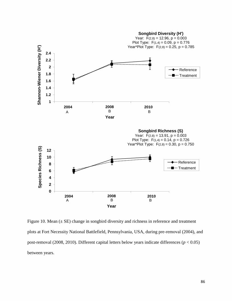
86

Figure 10. Mean (± SE) change in songbird diversity and richness in reference and treatment

plots at Fort Necessity National Battlefield, Pennsylvania, USA, during pre-removal (2004), and

post-removal (2008, 2010). Different capital letters below years indicate differences (p < 0.05)

between years.

1

1.2

1.4

1.6

1.8

2

2.2

2.4

Sh

an

no

n-W

ien

er

Div

ers

ity (

H')

Year

Songbird Diversity (H') Year: F(2,8) = 12.96, p = 0.003

Plot Type: F(1,4) = 0.09, p = 0.776 Year*Plot Type: F(2,8) = 0.25, p = 0.785

Reference

Treatment

2010 2004 2008 B B A

0

2

4

6

8

10

12

Sp

ec

ies

Ric

hn

es

s (

S)

Year

Songbird Richness (S) Year: F(2,8) = 13.91, p = 0.003

Plot Type: F(1,4) = 0.14, p = 0.726 Year*Plot Type: F(2,8) = 0.30, p = 0.750

Reference

Treatment

2010 2004 2008 A B B

87

Figure 11. Nonmetric multidimensional scaling (NMDS) ordination of songbird point count

surveys (Bray–Curtis matrix) from Fort Necessity National Battlefield, Pennsylvania, USA, in 3





0.05. FQI is code of the plant floristic quality index, H is for songbird species diversity, and S is

for songbird species richness.

88

Figure 12. Mean (± SE) change in total relative abundance, meadow jumping mouse, and white-

footed mouse densities, in reference and treatment plots at Fort Necessity National Battlefield,

Pennsylvania, USA, during pre-removal (2004 – 2006), and post-removal (2007 – 2010).

Different lowercase letters indicate differences (p < 0.05) within plot types across years.

Different capital letters indicate differences (p < 0.05) within a year, between plot types.

Different capital letters below years indicate differences (p < 0.05) between years.

0

5

10

15

2004 2005 2006 2007 2008 2009 2010

Ca

ptu

res/1

00

Tra

p

Nig

hts

Year

Sherman Trap Total Relative Abundance Year: F[6,12] = 15.67, p < 0.001


Reference

Treatment

B ACD BE ABCDE ACB C CD

0

1

2

3

2004 2005 2006 2007 2008 2009 2010

Ca

ptu

res/1

00

Tra

p

Nig

hts

Year

Meadow Jumping Mouse Relative Abundance Year: F[6,12] = 8.17, p = 0.001

Plot Type: F[1,4] = 0.67, p = 0.458 Year: F[6,12] = 1.97, p = 0.111

Reference Treatment

A A B B B B B

0

0.5

1

1.5

2

2.5

3

3.5

2004 2005 2006 2007 2008 2009 2010

Ca

ptu

res/1

00

Tra

p N

igh

ts

Year

White-Footed Mouse Relative Abundance Year: F[6,12] = 9.10, p = 0.001


Reference

Treatment

Ab

Aabd

Babcd Bab

Aabcd

Aa

Aabcd

Aabcde

Aad

Aa

Aace Aa

Aabcd

Abd

A A B B B B B

89

Figure 13. Mean (± SE) change in meadow vole densities from Sherman and pitfall traps, in

reference and treatment plots at Fort Necessity National Battlefield, Pennsylvania, USA, during

pre-removal (2004 – 2006), and post-removal (2007 – 2010). Different lowercase letters indicate

differences (p < 0.05) within plot types across years. Different capital letters indicate differences

(p < 0.05) within a year, between plot types. Different capital letters below years indicate

differences (p < 0.05) between years.

0

2

4

6

8

10

12

2004 2005 2006 2007 2008 2009 2010

Ca

ptu

res/1

00

Tra

p N

igh

ts

Year

Meadow Vole Sherman Trap Relative Abundance Year: F[6,12] = 13.23, p < 0.001


Reference

Treatment

Ba

Ab

Aa

Aa

Aa

Aa

Aa

Aa

Aa

Aa

Aa

Aa

Aa

Aa

0

5

10

15

20

25

30

35

40

45

2004 2005 2006 2007 2008 2009 2010

Ca

ptu

res/1

00

Tra

p N

igh

ts

Year

Meadow Vole Pitfall Relative Abundance Year: F[6, 24] = 4.63, p = 0.003

Plot Type: F[1, 4] = 19.60, p = 0.011 Year*Plot Type: F[6, 24] = 1.77, p = 0.147

Reference

Treatment

A A A B AB AB AB

90

Figure 14. Nonmetric multidimensional scaling (NMDS) ordination of small mammal Sherman

trapping (Bray–Curtis matrix) from Fort Necessity National Battlefield, Pennsylvania, USA, in 3




in years 2008 and 2010.Stress = 2.7 in the 3-dimensional solution. Vectors are significant at p ≤

0.05. Code is as follows: CPUE = captures/100 trap nights, C = plant coefficient of conservatism,

H = small mammal species diversity, J = small mammal species evenness.

91

Figure 15. Nonmetric multidimensional scaling (NMDS) ordination of small mammal pitfall

arrays (Bray–Curtis matrix) from Fort Necessity National Battlefield, Pennsylvania, USA, in 3




in years 2008 and 2010. Stress = 6.2 in the 3-dimensional solution. All vectors shown are

significant at p = 0.05. Code is as follows: FQI = plant floristic quality index.

92

CHAPTER 3

James T. Anderson

West Virginia University

Environmental Research Center

P O Box 6125

Morgantown, WV 26506 - 6123

304-293-3825; E-mail [email protected]

RH: Mammal use of exotic honeysuckle fruits

White-footed mouse (Peromyscus leucopus) selection of invasive bush honeysuckle fruits in

the Northeastern United States

Charneé L. Rose, Philip J. Turk, Stephen M. Selego, and James T. Anderson*

Division of Forestry and Natural Resources, Wildlife and Fisheries Resources Program,

West Virginia University, PO Box 6125, Percival Hall, Morgantown, WV 26506 (CLR, SMS,

JTA)

Department of Statistics, West Virginia University, PO Box 6330, Agricultural Sciences

Building, Morgantown, WV 26506 (PJT)

White-footed mice (Peromyscus leucopus) are influential in the consumption and

distribution of seeds and fruit of native plants; however, little is known about their interactions

with exotic shrubs. Depending on foraging activity, this species could represent an essential

element of resistance against exotic plants, contribute to their spread, or have no impact. Use of

invasive Morrow‟s honeysuckle (Lonicera morrowii) and 5 native soft mast species was studied

across 3 cover types (forest, field, and edge) and 2 survey rounds (October – November 2009 and

July – early August 2010) in southwestern Pennsylvania, USA. Feeding stations, containing

equal quantities of each species, were randomly placed in each of the 3 cover types (n = 20).

Honeysuckle was always present, but native species differed based on availability. In addition,

----------------

*Correspondent: [email protected]

This manuscript written in the style of the Journal of Mammalogy

93

nutrient composition, total energy, seed number, mass, and handling time were measured. Fruit

consumption was non-random based on compositional analysis (P < 0.05). Honeysuckle was

consumed over native staghorn sumac (Rhus typhina) in July – early August. Otherwise, it was

consumed less than all natives. Honeysuckle fruits had significantly less protein (0.66%) and

lipids (0.67%) than all natives (P < 0.05). Total energy was important in distinguishing the

highest selected fruits: black cherry (Prunus serotina) (0.45 kcal), and common dewberry (Rubus

flagellaris) (0.36). Use of fruits beyond the first chosen was inconsistent and varied based on

moisture, protein, lipids and carbohydrates. Average seeds and mass per fruit, and handling time

had no influence on use. White-footed mice show plasticity in their diets with the ability to

optimize trade-offs in nutrient content across seasons. Natives in the invaded landscape appear to

experience higher consumption pressures on their fruits, and we conclude that Morrow‟s

honeysuckle creates a monoculture of a lesser-used, and likely a lesser-preferred, food item.

Key words: compositional analysis, diet selection, foraging preference, invasive species, soft

mast

---------------------------------------------------------------------------------------------------------------

Widespread attention has been paid to global trade and travel as potential pathways of

invasive species spread (Hulme 2009). However, ecological pathways of persistence (such as

wildlife spread of exotic plant seeds) are rarely studied (Edalgo et al. 2009; Shahid et al. 2009;

Williams et al. 1992). Generalist granivore species, Peromyscus, are widely distributed across

the United States (Hall 1980; Kantak 1983). Small mammals, including white-footed mice

(Peromyscus leucopus) are the dominant consumers of fruit and seeds in both forests (Schnurr et

al. 2002) and fields (Bowers and Dooley 1993; Manson et al. 1999; Ostfeld et al. 1997). Schnurr

et al. (2004) and Ostfeld et al. (1997) found that Peromyscus influence the spread and survival of

seedlings into a number of habitats. The diet of white-footed mice in northern latitudes is heavily

94

dominated by fruits and seeds, especially during colder months (Wang et al. 2009). During

autumn months, Peromyscus cache fruits in a manner that increases germination potential

(Vander Wall et al. 2001). It is possible, given dietary needs and preference, that Peromyscus

could assist in the spread of invasive plants or contribute little to their population dynamics.

Since being introduced from Japan as an ornamental (Luken and Thieret 1995; Rehder

1940), Morrow‟s honeysuckle (Lonicera morrowii) has become a persistent invasive shrub in the

northeastern United States. Morrow‟s honeysuckle occupies a wide range of cover types

including riparian areas, early successional fields (McClain and Anderson 1990), forest interiors

(Woods 1993), edges, and corridors. This shrub also occupies areas of disturbed land including

roadsides, railroads (Barnes and Cottam 1974), and abandoned agricultural land (Hauser 1966).

A variety of studies have examined the impacts of invasive plants on native ecosystems.

Although studies are lacking that examine the effect of exotic plants on small mammal

populations, Edalgo et al. (2009) conducted a study on the effects of Morrow‟s honeysuckle on

small mammal microhabitat selection. This study found that white-footed mice selected areas

with shrub cover, including that from Morrow‟s honeysuckle, when compared to random trails.

If white-footed mice are selecting areas with Morrow‟s honeysuckle cover, then this could

equate to foraging activity in these areas, and potentially indicate consumption of this invasive

species. It is important to determine consumption rates (compared to native species as

references) as they could be a factor in the pervasive spread of this invasive species. Also,

because Morrow‟s honeysuckle is known to outcompete both native herbaceous and shrub

species (Batcher and Stiles 2000) it is critical to determine if it is used as a replacement food

source or if it creates vast monocultures of a less consumed food source. The objectives of our

study were to: 1) determine the rate of consumption of Morrow‟s honeysuckle when compared to

95

that of available native species; 2) assess the magnitude of selection across cover types; 3) and

identify fruit characteristics (nutritional content, seed number, mass, and handling time) which

may affect use.

MATERIALS AND METHODS

Study site. – Research was conducted at Fort Necessity National Battlefield (FONE),

located in Fayette County in southwestern Pennsylvania, U.S.A. (39º48‟43” N, 84º 41‟50” W).

FONE is situated in the Laurel Highlands portion of the Allegheny Mountains subregion of the

Appalachian Plateau. Elevations throughout the 390 ha park range from 535 – 710 m. The

average annual temperature is 9º C, the mean winter temperature is -3º C, and the mean summer

temperature is 22º C. The average precipitation level is 119 cm (National Park Service 1991).

Deep, poor to moderately drained soils (Philo silt loams) characterize the low laying areas within

the park. Moderately deep, moderate to well drained soils (Brinkerton and Armagh silt loams,

Cavode silt loams, and Gilpin channery silt loams) characterize the upland sites within the park

(Kopas 1973).

The FONE landscape has undergone a variety of alterations. The park was once

dominated by an oak-hardwood forest in the mid-1700s. The land was cleared for livestock

grazing prior to the establishment of FONE in 1933. After acquisition of the area the National

Park Service actively managed by mowing until the mid-1980s. It was believed that if mowing

ceased it would allow the pasture to return to forested conditions. However, with passive

management, the area became dominated by a dense cover of Morrow‟s honeysuckle and other

exotic species (National Park Service 1991). During a survey of FONE fields, mean percent

frequency of 93 plant species was calculated from 225 1 x 1 m vegetation samples and showed

that Morrow‟s honeysuckle occurred at 92% of the sites (Love 2006). This frequency was greater

than any native or invasive plant species known at the study site.

96

Cover types on FONE include field, wet meadow, oak-hardwood forest, coniferous

forest, wetland, ephemeral stream, and natural and induced edge. This study was conducted

across 3 of the dominant cover types: oak-hardwood forest, induced edge, and field. Edges were

forested areas located within 10 m of park roads. The forest interior were forested areas 100 m in

from the woodland edge or from any human-created opening (Laurance et al. 2001). The forest

was comprised of mixed-hardwoods dominated by northern red oak (Quercus rubra) and yellow

poplar (Liriodendron tulipifera). Fields were early successional areas dominated by various grass

species (Dactylis spp., Phleum spp.), sedges (Carex spp.), and goldenrods (Solidago spp.).

Foraging stations. – We used cafeteria-style food boxes (36 x 21 x 21 cm), constructed

from 1.5 cm thick plywood and 1.5 cm aperture wire mesh to allow for camera monitoring of

feeding activity (Fig. 1). Each box had a single 5 x 5 cm square hole at ground level to provide

access to small mammals (Shahid et al. 2009). Small mammal movements were not confined

during feeding trials; individuals could visit multiple stations or forage freely outside of the

stations. Four weigh boat dishes (4.6 x 4.6 cm) (Avogadro's Lab Supply Inc., Miller Place, New

York) were housed in each box. All foraging stations were staked to the ground with 15 cm lawn

staples and metal connecting plates to avoid disturbance by raccoons (Procyon lotor) or other

non-target species. Sixty stations were randomly placed based on cover type (strata) with 20 in

each. Each station was spaced ≥ 100 m apart to ensure statistical independence (Fig. 2) (Pearson

et al. 2001; Williams 2002).

Fruit selection. – This study took place during 2 rounds: October 20 – November 14,

2009 at a time when soft mast natives were abundant in the environment (Round 1), and July 12

– August 6, 2010 when native soft mast was limited (Round 2). Natives were chosen at random

from 9 species during Round 1, and from 3 species during Round 2, using a random number

97

generator in Microsoft Excel (Appendix Ib). When a fruit species could not be located in

sufficient numbers another species was randomly selected as a substitute. During the early

summer sampling period the native fruit mast available was limited. Therefore, there were only 2

native species available for use: northern dewberry (Rubus flagellaris), and staghorn sumac

(Rhus typhina). During the fall sampling period the native fruit mast consisted of black cherry

(Prunus serotina), southern arrowwood (Viburnum dentatum), and winter grape (Vitis cinerea).

Fruits were picked when ripened, from at least 3 plants, and within a 3-day period of the first

pick. Fruit samples were frozen at -20º C at the FONE Natural Resources Research Station (until

food trials), and at West Virginia University (until processed for nutrient composition).

Consumption monitoring. – Each of the fruit selection rounds in the study lasted a total of

20 days, excluding a 5-day pre-baiting period when rolled oats and peanut butter were placed in

each box (Shahid et al. 2009) to encourage small mammal visitation. We placed the fruits (n = 7

per species) in separate dishes in a random order nightly. Cafeteria boxes were checked every 24

h. The number and condition of fruits and seeds remaining were recorded, cleared from the site

and replenished. All berries were replaced regardless of non-consumption or condition. This was

done to eliminate bias of selection based on the time individual fruits had been placed in the box.

Nutrient composition and metrics. – For each fruit species we measured percent moisture,

ash, fat, crude protein (CP), neutral detergent fiber (NDF) (cellulose, hemicelluloses, and lignin),

and nonfiber carbohydrates (NFC) (starches, sugars, fructans, and pectins). Each of the following

procedures was performed in 3 rounds consisting of subsamples taken from a larger 10 – 20 g

sample depending on moisture content (n = 30 – 600 fruits per sample). Percent moisture was

determined from weights before and after drying a 10 – 20 g sample. Fat content was directly

measured using a 0.50 g sample of each fruit placed in 26 x 60 mm Whatman® Cellulose

98

Extraction Thimbles (Whatman Incorporated, Piscataway, New Jersey) and refluxed with

petroleum ether in a TecatorTM

Soxtec Apparatus (Rose Scientific, Alberta, Canada) (Dobush et

al. 1985). Nitrogen content was measured using a 0.50 g sample of each fruit placed in a

digestion tube (250 ml) in a TecatorTM

Digestion System (Rose Scientific, Alberta, Canada),

followed by a Kjeldahl Auto 1030 Analyzer (Foss Tecator, Hoganas, Sweden) with automatic

distillation and titration. We then estimated crude protein content as: [% nitrogen x 4.4] (Smith et

al. 2007; Witmer 1998). Neutral detergent fiber was directly measured using a 0.25 g sample for

each fruit following the Ankom Analyzer procedure, using an Ankom200

Fiber Analyzer

(ANKOM Technology, Fairport, New York) (Getachew et al. 2004). Total nonfiber carbohydrate

(TNC) was calculated as: [100% - (% fat + % ash + % CP + % NDF)] (Smith et al. 2007).

Calculating NDF allowed us to distinguish between structural and nonstructural carbohydrates.

Samples were then placed in a 600º C furnace for 2 h to oxidize all organic matter, allowing us to

weigh the resulting inorganic residue to determine ash. Total energy (kcal) was calculated for

each species as: [((% NFC x 4) + (% CP x 4) + (% fat x 9)) x fruit mass] (Atwater and Bryant

1900).

We dissected 100 fruits of each species to determine the average seed number per fruit

(Williams et al. 1992). Using a Scout ProTM

SP202 portable bench scale (capacity 200 x 0.01 g)

(Totalcomp Scales & Balances, Fair Lawn, New Jersey) we weighed 100 samples of fruits to the

nearest gram to establish the wet mass of each fruit species. To reduce scale error, all species

were weighed in subsamples of 25 (except staghorn sumac, n = 50) due to the low mass of

individual fruits.

Small mammal surveys. – Collapsible Sherman live traps (Large Folding Galvanized

(LFG), 7.5 x 8.9 x 23 cm), were used to determine small mammal species composition. Trapping

99

began after the final day of the selection study, and spanned over 4 consecutive days. Rolled oats

and peanut butter were placed in each trap (Shahid et al. 2009), along with cotton to minimize

exposure to weather extremes. Traps were opened daily at 1600 h, and checked and closed at

0600 h, to allow for detection of both diurnal (e.g., eastern chipmunks, Tamias striatus) (Aschoff

1966) and nocturnal species while minimizing mortality and stress (Sikes et al. 2011). Every

mouse and vole received a #1005-1 model ear tag (National Band and Tag Company, Newport,

Kentucky 41072-0430). Shrews were toe clipped. Animals were released at the trap station

where they were caught.

Sherman traps were associated with each of the 60 foraging stations; 1 trap placed

directly at the box, 1 trap spaced 33 m and another 66 m away from each box. This trap spacing

makes the second trap spaced 66 m away from the first box, but only 33 m away from the next

box (if present), keeping the trap spacing consistent (n = 60/per cover type). This system was

employed to determine if the boxes were separated through the captures of individual mammals.

Camera monitoring units were used to confirm live trapping results, as well as to survey

the foraging times and preferences of soft mast. A camouflaged camera with articulating arm,

and a 12-volt deep-cycle marine battery were used in each cover type, nightly, randomly

assigned to 1 of the 20 cafeteria box positions. The units consisted of a video camera connected

to a recorder in a weatherproof case (Fuhrman Diversified, Seabrook, Texas) by a 20 m cable.

The system used infrared light to allow filming during nocturnal foraging bouts without

disrupting the animals‟ natural behaviors.

The articulating arm was used to position the cameras on the ground, 20 cm from the

wire-mesh wall of the box, in clear view of the seed dishes and to allow for adequate lighting.

Where possible, the video recorder and battery were placed behind habitat structures (logs, trees,

100

rocks, etc.) and up to 10-15 m away from the box. We changed the videotape daily and replaced

the battery every 24 – 48 h. Monitoring was started between 1800 – 2000 h, at the beginning of

an active foraging period for the white-footed mouse (Williams et al. 1992). Monitoring

extended until 0200 to 0400 h as tapes have an 8 h maximum recording capacity. Although other

studies have had success with using time-lapse recording to extend their taping efforts a full 24 h

(Stake et al. 2004; Thompson and Burhans 2003), we did not alter the standard recording frames

in order to get a reliable calculation for handing time of each fruit species. Handling time was

calculated for all fruits through visual monitoring of foraging activity, and was defined as the

time it look a small mammal to completely consume a chosen fruit. The video footage obtained

from the camera monitoring was viewed for the following information: 1) species identification,

2) time the individual entered, 3) type and number of each fruit selected, 4) handling time for

each fruit, and 5) time individual exited the station.

The opening of the cafeteria boxes were saturated in fluorescent tracking powder (Edalgo

et al. 2009). The pigment saturated the fur of the animals (2-4 μm; Radiant Color, Inc), and

allowed us to return with an ultraviolet 6 Watt Long-Wave Lamp (Edalgo et al. 2009) to identify

species‟ tracks. This allowed us to fine-tune the analysis and exclude any trial nights for a

particular station that had been used by a non-target species (any mammal larger than 120 g,

songbirds, etc.).

Research was conducted under the National Park Service (NPS) research permit FONE-

2009-SCI-0002. Animal handing followed protocols approved by the Animal Care and Use

Committee at West Virginia University, protocol number 09-0905. This study met guidelines of

the American Society of Mammalogists (Sikes et al. 2011) for proper handling of study species.

101

Diet analysis. – We used compositional analysis (CA) and multivariate techniques to

determine if the small mammal species surveyed were using mast resources more frequently than

would be expected by chance given their relative availability. We used α = 0.05 for all tests

unless otherwise noted. We calculated the proportions of use for each fruit species, and a

category of unconsumed fruits (UNCON), for each of the 60 boxes, after pooling the data from

all trial days. Because all fruits were available in equal proportions in the study, selection

probability was standardized across all species, and the UNCON category (100/number of

foraging categories). The UNCON category was necessary to examine consumption differences

among habitats. For a given study box, the consumption of the various foraging categories are

not considered independent since if the consumption of one fruit increases, the consumption of

another decreases (Aitchison 1986; Pendleton et al. 1998). Therefore, the analysis converted the

proportions to log-ratios, and in instances when proportions equaled zero a small constant was

added (0.01) (Aebischer et al. 1993). Our analysis compared use and availability of each fruit

species to an arbitrary reference class by differencing log-transformed ratios of species

proportions for each foraging box (Aitchison 1986; Aitchison 1994), following the methods

described in Dickson and Beier (2002). A matrix ranking foraging categories was constructed

when mast use was found to be nonrandom, and t-tests were performed to compare use between

foraging categories.

Morrow‟s honeysuckle and UNCON were used as reference categories during

multivariate analysis of variance (MANOVA) testing. The MANOVA was used to test if mean

numbers of fruits consumed were consistent across cover types. When a significant MANOVA

was observed, a series of univariate analysis of variance (ANOVA) tests were performed.

102

When the ANOVA F-test was significant, pairwise comparisons of cover types were examined

through Tukey‟s multiple comparisons procedure. Residual diagnostics were performed to

assess the validity of the model assumptions. In some instances, permutation tests were used to

confirm previous results when a departure from the normality assumption was noted.

Nutrient and mammal community composition analysis. – We used MANOVA to

determine if there were significant differences in nutrient composition, seed number, and mass

among the various fruit species. This same method was used to determine if there were

differences between total relative abundance, measured as captures/100 trap nights (CPUE), and

the relative abundance of the 2 most dominant small mammals captured across cover types. We

deducted 0.5 trap nights for each trap tripped without a capture and each with a non-target

species (Beauvais and Buskirk 1999; Edalgo and Anderson 2007).

Following a significant MANOVA result, we performed a series of ANOVA tests. When

the ANOVA F-test was significant, pairwise comparisons were examined through Tukey‟s

multiple comparisons procedure. Percent moisture, fat, and crude protein composition of fruits

and relative abundance of meadow voles (Microtus pennsylvanicus) (during all study rounds)

were found to be in violation of parametric assumptions and were square root transformed.

Based on the camera monitoring we calculated the following descriptive statistics: total

species abundances, total of each fruit species selected, average time foraging began, and

average time foraging ended. Additionally, we calculated average handling time for fruit species

by individual small mammal species. When the same individual was seen consuming multiples

of a species we averaged the times for that individual. Due to low and unequal sample sizes, we

used a Kruskal-Wallis one-way analysis of variance test to determine differences in handling

time for each fruit species. Handling time was only analyzed for white-footed mice due to few

103

observations of other species at foraging stations. Given a significant result, pairwise

comparisons were examined through a series of Bonferroni corrected (α = 0.002) Mann-Whitney

U tests.

RESULTS

Small mammal community composition. – When pooling all trapping efforts between

rounds there were a total of 1,330 trap nights after deductions, with 289 total captures. Out of

211 unique individuals, 187 were white-footed mice (88.63%). Other species captured included:

meadow vole (n = 11 captures, 5.21%), northern short-tailed shrew (Blarina brevicauda, n = 5,

2.37%), woodland vole (Microtus pinetorum, n = 4, 1.90%), meadow jumping mouse (Zapus

hudsonius, n = 2, 0.95%), masked shrew (Sorex cinereus, n = 1, 0.47%), and southern bog

lemming (Synaptomys cooperi, n = 1, 0.47%). White-footed mice were also the dominant species

observed during camera monitoring (Table 1). White-footed mice comprised 77% of the camera

observations in Round 1, and 84% in Round 2. The average length of a visit to a foraging station

by a white-footed mouse was 1.67 min. ± 0.19 in Round 1, and 2.22 ± 0.51 in Round 2. The

eastern chipmunk (n = 3) was the only species observed with cameras that was not captured

through Sherman live trapping. We never identified songbird species in the fluorescent powders,

and we did not capture any on camera footage. Although, raccoons were captured on film, they

were not seen disturbing the foraging boxes, so no trial nights for any station needed to be

excluded.

Capture rates varied among cover types in Round 1 (Wilks‟ λ2 = 0.13, F6,14 = 4.20, P =

0.013) and Round 2 (λ2 = 0.07, F6,14 = 6.42, P = 0.002) (Table 2). There were no differences in

total captures across cover types in Round 1 (F2,9 = 1.29, P = 0.321) or in Round 2 (F2,9 = 1.94,

P = 0.199). There was no difference in white-footed mouse relative abundance across cover

104

types in Round 1 (F2,9 = 0.55, P = 0.596); however, in Round 2 fewer mice were captured in

fields when compared to edges (F2,9 = 5.47, P = 0.028). In Round 1 meadow voles had higher

relative abundance in fields when compared to all other cover types (F2,9 = 9.00, P = 0.007); the

same relationship was seen in Round 2 (F2,9 = 21.14, P < 0.001).

Fruit use. – Fruit use was non-random based on a global test of selection during Round 1

(Wilks‟ λ4 = 0.12, P < 0.001), and Round 2 (λ3 = 0.19, P < 0.001); foraging categories were

ranked in order of preference for both rounds (Table 3):

Round1: Unconsumed > Cherry > Arrowwood > Grape > Honeysuckle; and

Round 2: Unconsumed > Dewberry > Honeysuckle > Sumac.

These same patterns of use were also seen, for each round, through camera monitoring at the

foraging stations (Table 1). In Round 1, black cherry comprised 51% of the observed

consumption, southern arrowwood 35%, winter grape 14% and Morrow‟s honeysuckle < 0.5%.

In Round 2, northern dewberry comprised 56% of the observed consumption, Morrow‟s

honeysuckle 29%, and staghorn sumac 15%.

Although the pattern of use did not differ across cover types during any round,

consumption within a species (compared to total unconsumed fruits) and the magnitude of use

(i.e., the difference between the mean numbers of fruits consumed compared to honeysuckle) for

species varied across cover types in Round 2 (Wilks‟ λ2 = 0.60, F6,110 = 5.26, P < 0.001 for both

tests due to functional dependency) (Table 4). Less honeysuckle was consumed in the field than

in edge or forest boxes (F2,57 = 10.15, P < 0.001), with no difference between edge and forest.

Northern dewberry experienced less consumption in the field compared to other cover types

(F2,57 = 5.31, P = 0.008). Staghorn sumac also experienced less consumption in the field when

compared only to edge boxes (F2,57 = 4.96, P = 0.010), with no differences between edge and

forest, and field and forest. The use of Morrow‟s honeysuckle over staghorn sumac was

105

increased in the forest when compared to both edge and field (F2,57 = 7.95, P < 0.001), with no

difference between edge and field. There was no variation in the magnitude of use between

northern dewberry and Morrow‟s honeysuckle across cover types (F2,57 = 1.86, P = 0.165).

There was no variation in consumption within a species or magnitude of use between a native

and honeysuckle across cover types in Round 1 (λ2 = 0.76, F8,108 = 1.99, P = 0.055) (Table 4).

Fruit species characteristics. – There was variation (λ5 ≈ 0.00, P < 0.001) in the

nutritional composition (F35,28 = 397.61, P < 0.001), seed number and mass (F10,1186 = 7699.20, P

< 0.001). Among fruit species there were differences in all characteristics measured: fat (F5,12 =

650.05, P < 0.001), moisture (F5,12 = 674.19, P < 0.001), NDF (F5,12 = 193.88, P < 0.001), ash

(F5,12 = 8.77, P = 0.001), crude protein (F5,12 = 208.43, P < 0.001), NFC (F5,12 = 58.43, P <

0.001), total energy (kcal) (F5,12 = 1042.20, P < 0.001), seeds per fruit (F5,594 = 10675, P <

0.001), mass per fruit (F5,594 = 23769, P < 0.001), and handling time (χ2

5 = 27.19, P < 0.001)

(Table 5). During Round 1, black cherry was consumed highest; it had the highest kcal, protein,

and non-fiber carbohydrates. Morrow‟s honeysuckle, used least often, had the highest moisture

content, seed count, and mass, but the lowest fat, protein, and kcal. Handling time was not

different between species. During Round 2, northern dewberry was consumed highest; it had the

highest kcal, handling time, seed number and mass. The most utilized items, dewberry and

honeysuckle, had statistically identical moisture content, which was higher than the least

consumed fruit (staghorn sumac). Sumac had the highest protein, but the lowest kcal and

handling time.

106

DISCUSSION

Characteristics affecting use. – We determined that the fruits of Morrow‟s honeysuckle

were generally least consumed when compared to native species; although, it is as important to

understand the characteristics about the fruits (other than invasiveness) that may have

contributed to use. Our study verified that white-footed mice did not forage randomly, but

individuals still consumed portions of all fruits available. Vickery et al. (1994) found a similar

result and concluded that deer mice (Peromyscus maniculatus) appeared to sample a variety of

foods on a daily basis to determine which had the greatest nutritional value. Although white-

footed mice may exhibit similar behavior when foraging, certain fruit characteristics did stand

out during the study. The highest consumed fruit from each round was always a native species,

and had the highest total energy content available. Energy gained from consuming fat, protein,

and carbohydrates is used for thermoregulation, growth, movement, and reproduction (Bryant

and Tatner 1991). Lewis et al. (2001) found that white-footed mice used the highest-energy

foods regardless of the amount of protein found in them. This result was seen in our study, with

the addition that the amount of lipids and carbohydrates also appeared to be secondary to total

energy.

High use also seemed to coincide with a need for water resources. Many animals rely on

water in food because drinking water may be scarce and drinking may increase other risks to

survival such as depredation (Maloney and Dawson 1998; Withers 1992). Our study was

conducted within the breeding season for white-footed mice, which occurs from March until

November (Wolff 1985). Breeding peaks in this species appear to correspond to instances where

water intake and dietary protein were important; water and protein losses occur during lactation

when water is lost during milk production (Barboza et al. 2009).

107

Temporal variation in characteristics. – White-footed mouse diets during the summer

may be predominantly arthropod-based (high-protein foods), and during this season consumption

of fruits and green vegetation (high-water foods) are considerably higher than during autumn

when hard-mast consumption is increased (Wolff et al. 1985). Protein catabolism produces the

solute urea, which increases urinary water loss in attempts to remove this toxic byproduct

(Barboza et al. 2009), increasing the need for water during the summer. Although the most

protein-rich fruit was not highly used during Round 2 (summer), high protein ingestion from the

environment may explain the consumption of fruits such as dewberry and honeysuckle, which

were high in water content.

Variation in the environment can change the availability and demand of both water and

nutrients (Barboza et al. 2009). Although the pattern of use did not indicate that they were

choosing fruits based solely on individual amounts of protein, fat, carbohydrates, etc., these

nutrients appear to be important during specific rounds. Protein, fat, and carbohydrates seemed

particularly important in Round 1 (autumn), while moisture content was more prominent in

Round 2. This indicates that during the autumn, when high foraging activity was taking place in

preparing for winter, easily digested sugars (quick energy) were important, and during breeding

peaks lipids containing more energy and protein providing nitrogen for antibodies were

important (Barboza et al. 2009).

Characteristics with low influence on use. – There were a number of characteristics that

seemed to provide no influence on use. Average seeds and mass per fruit lacked importance in

the study with the exception of the highest consumed species, dewberry, in Round 2. The use of

this species is likely most attributed to it being highest in total energy (Lewis et al. 2001), and its

high seed count is a potential side-effect. Likewise, Morrow‟s honeysuckle was second in mass

108

and seeds only to dewberry and it experienced the lowest consumption when compared to all

other fruits, except staghorn sumac. In an effort to consider the trade-off between energy

expended during consumption and nutrients obtained we calculated the handling time for each

species. However, any discernible pattern of use seemed to have little to do with this variable.

Additionally we looked at patterns between total energy per gram of fruit, and total energy when

compared to energy expenditure, and no additional information was revealed. Previous studies

have also found no correlation between the diet of white-footed mice and the seed size, number,

mass or hardness (Ivan and Swihart 2000; Kaufman and Kaufman 1989; Shahid et al. 2009), and

when a highly used food item was removed individuals increased use of non-utilized food items.

This ability to use a previously lower consumed food source could explain the use of

honeysuckle in Round 2. There were fewer natives in the environment during this time (early

summer), and this corresponds to what appears to be the highest consumption of this invasive

species.

Additional factors affecting foraging. – All of the species used in the study were available

in the environment outside of the foraging boxes. Due to aggressive spread, Morrow‟s

honeysuckle was the most common study species in field habitats. We don‟t think that

honeysuckle saturation in particular cover types confounded the results, leading to greater use of

less-common natives. The consumption pattern of native fruits over honeysuckle fruits was

consistent between the 3 cover types, including the forest where honeysuckle was nearly absent.

Fruits and seeds can constitute a large proportion of small mammal diets (Martin et al.

1961). Therefore, the number of fruits left unconsumed in the study boxes throughout the rounds

was surprising. With closer inspection of the data, we found that there were instances when

specific foraging boxes were rarely (≤ 2) or never visited by small mammals. The ability to

109

forage may change due to weather conditions or threat of depredation (Barboza et al. 2009; Dutra

et al. 2011). In addition, animals need to care for offspring, rest, and interact with other

components of their environment (Caro 2005). Time for feeding activity could have been

restrained and have affected the unconsumed totals depending on favorable environmental

conditions. Along with the study species, there was a variety of alternative food sources available

outside of the study boxes. It is therefore likely that study stations were in competition with other

surrounding food sources in the environment. This directly relates to field boxes experiencing

lower consumption rates during Round 2, as many were inundated with grass seed. It is likely

that the saturation of grass seed is responsible for low consumption rates, due to a competing

food source. Since predation risk is often regarded as one of the most pervasive factors affecting

foraging activity of small mammals (Ebersole and Wilson 1980; Manson and Stiles 1998), it may

be of interest to study the environmental variables that contribute to high visitation success to

foraging stations.

Morrow’s honeysuckle fruit characteristics. – Although honeysuckle is classified as a

low quality browse food (White and Stiles 1992), Morrow‟s honeysuckle was in the mid-range

of values for non-fiber carbohydrates and total energy available, while having one of the highest

moisture contents of study fruits. Its moisture content appears to be important in its use by white-

footed mice, a result not previously documented due to the availability of only dried seeds in

prior feeding trials. Otherwise, the fruits are lower in fat and protein than any other species used

in the study, results consistent with Witmer and Van Soest (1998). This means they are lacking

key nutrition for survival and reproduction. The fruits of Morrow‟s honeysuckle contain

compounds, such as iridoid glucosides (Ikeshiro et al. 1992), which can deter grazing herbivores.

Although our study has already identified a number of factors that both favor and deter selection

110

of honeysuckle, it is likely that defensive compounds play a role in avoidance of this species, and

should be further evaluated.

Dominant species and monitoring techniques. – Through multiple sampling techniques

we determined that the dominant small mammal species was the white-footed mouse. Evidence

does not support that consumption of fruit was confounded by the community composition of

small mammals due to the low abundances of other species and the generally consistent relative

abundance of white-footed mice across cover types. While there was a decrease observed in the

captures of white-footed mice during Round 2 in fields when compared to other cover types; this

also coincided with a general decrease in consumption rates in that cover type. Therefore, we are

confident in attributing fruit consumption to this species. They are habitat generalists (Adler and

Wilson 1987; Dueser and Shugart 1978) known to have a greater dietary breadth than many

granivores, which explains the ready consumption of all fruit species in the study (Lackey et al.

1985). We used foraging stations that would likely not alter mammal behavior or impede their

movements to attain a more accurate picture of consumption (Connors et al. 2005). Our spacing

of ≥ 100 m between boxes generally sufficed for independence; although some individuals were

captured at more than 1 box, or closer than 33 m to a neighboring box. In the few instances

where cameras captured other species foraging (specifically eastern chipmunks and meadow

voles), their consumption of honeysuckle appeared to match those of white-footed mice. Other

species captured on the monitoring units did not consume fruits from the foraging boxes. In

nearly all instances seen on film, small mammals consumed the whole fruit (not just the seeds)

while in the box; few were carried outside of the box. This confirmed our decision to use whole

fruits at the stations, and to conduct nutritional analysis on the entire fruit.

111

Nutrition and energy expenditure. – The relation between food abundance and

consumption can determine an animal‟s energy intake; the more abundant a food source is, the

more likely it is to be discovered during foraging activity (Barboza et al. 2009). Animals with

high metabolic rates, such as small mammals, may be unable to sustain prolonged searches for

food, especially if the food source has low abundance or is of low quality (Barboza et al. 2009).

This appears to be the case with invasive Morrow‟s honeysuckle, as it is low in vital nutrients,

and creates vast monocultures reducing natives from the environment, which are the higher

consumed food sources. This in turn may force small mammals, like white-footed mice, to

forage for longer periods of time, or travel further distances and increase their risk of

depredation. While white-footed mice showed plasticity in their diets with the ability to optimize

(utilize the fruits with the highest total energy) between trade-offs in nutrient content across

seasons, it is likely that this species is pressured by large energy expenditures to find suitable

food sources. Natives in the invaded landscape experience higher consumption rates on their

fruits, and although this shrub provides cover for small mammals (Dutra et al. 2011; Edalgo et al.

2009), we conclude that Morrow‟s honeysuckle creates a monoculture of a less nutritious and

less used food item.

ACKNOWLEDGMENTS

Funding was provided by the NPS, and the WVU Environmental Research Center. For assistance

in the field, we thank J. M. Holmes, J. De La Cruz, F. Klinger, and W. Riley. We thank G.

Merovich for statistical guidance and consultation. We thank T. Webster from the WVU Rumen

Fermentation Profiling Lab for nutritional analysis of the fruit species. The foraging stations used

for monitoring were kindly produced by P. Ludrosky. Grateful acknowledgement is made to the

staff at FONE, particularly C. Ranson for her logistical support and encouragement. This is

112

scientific article number xxxx of the West Virginia University Agricultural and Forestry

Experiment Station.

LITERATURE CITED

ADLER, G. H., AND M. L. WILSON. 1987. Demography of a habitat generalist the white-footed

mouse, in a heterogeneous environment. Ecology 68:1785–1796.

AEBISCHER, N. J., P. A. ROBERTSON, AND R. E. KENWARD. 1993. Compositional analysis of

habitat use animal radio-tracking data. Ecology 74:1313–1325.

AITCHISON, J. 1986. The statistical analysis of compositional data. Chapman and Hall, London,

England, 416 pp.

AITCHISON, J. 1994. Principles of compositional data analysis. Multivariate Analysis and Its

Applications 24:73–81.

ASCHOFF, J. 1966. Circadian activity pattern with two peaks. Ecology 47:657–662.

ATWATER, A. O., AND A. P. BRYANT. 1900. Availability and fuel values of food materials.

Connecticut Agricultural Experimental Research Station Annual Report 12:73–100.

BARBOZA, P. S., K. L. PARKER, AND I. D. HUME. 2009. Integrative wildlife nutrition. Springer,

Heidelberg.

BARNES, W. J., AND G. COTTAM. 1974. Some autoecological studies of the Lonicera × bella

complex. Ecology 55:40–50.

BATCHER, M. S., AND S. A. STILES. 2000. Element stewardship abstract for Lonicera maackii



(Bell‟s honeysuckle). The Nature Conservancy, Arlington, Virginia. Available from

113

http://www.imapinvasives.org/GIST/ESA/esapages/documnts/loni_sp.pdf (accessed

September 2009).

BEAUVAIS, G. P., AND S. W. BUSKIRK. 1999. Modifying estimates of sampling effort to account

for sprung traps. Wildlife Society Bulletin 27:39-43.

BRYANT, D. M., AND P. TATNER. 1991. Intraspecies variation in avian energy expenditure:

correlates and constraints. Ibis 133:236–245.

BOWERS, M. A. AND J. R. DOOLEY, JR. 1993. Predation hazard and seed removal by small

mammals: microhabitat versus patch scale effects. Oecologia 94:247–254.

CARO, T. 2005. Antipredator defenses in birds and mammals. University of Chicago Press,

Chicago, Illinois.

CONNORS, M. J., E. M. SCHAUBER, A. FORBES, C. G. JONES, B. J. GOODWIN, AND R. S.

OSTFELD. 2005. Use of track plates to quantify predation risk at small spatial scales.

Journal of Mammalogy 86:991–996.

DICKSON, B. G., AND P. BEIER. 2002. Home-range and habitat selection by adult cougars in

Southern California. The Journal of Wildlife Management 66:1235–1245.

DOBUSH, G. R., C. D. ANKNEY, AND D. G. KREMENTZ. 1985. The effect of apparatus, extraction

time, and solvent type on lipid extractions of snow geese. Canadian Journal of Zoology

63:1917–1920.

DUESER, R. D., AND H. H. SHUGART. 1978. Microhabitats in a forest-floor small mammal fauna.

Ecology 59: 89–98.

DUTRA, H. P., K. BARNETT, J. R. REINHARDT, R. J. MARQUIS, AND J. L. ORROCK. 2011. Invasive

plant species alters consumer behavior by providing refuge from predation. Oecologia

165:1–9.

114

EBERSOLE, J. P., AND J. C. WILSON. 1980. Optimal foraging: the responses of Peromyscus

leucopus to experimental changes in processing time and hunger. Oecologia 46:80–85.

EDALGO, J. A., AND J. T. ANDERSON. 2007. Effects of prebaiting on small mammal trapping

success in a Morrow‟s honeysuckle-dominated area. Journal of Wildlife Management

71:246–250.

EDALGO, J. A., H. M. MCCHESNEY, J. P. LOVE, AND J. T. ANDERSON. 2009. Microhabitat use by

white-footed mice Peromyscus leucopus in forested and old-field habitats occupied by


GETACHEW, G., P. H. ROBINSON, E. J. DEPETERS, AND S. J. TAYLOR. 2004. Relationships

between chemical composition, dry matter degradation and in vitro gas production of

several ruminant feeds. Animal Feed Science and Technology 111:57–71.

HAUSER, E. J. P. 1966. The natural occurrence of a hybrid honeysuckle (Lonicera × bella) in

Ohio and Michigan. Michigan Botanist 5:211–217.

HALL, E. R. 1980. The mammals of North America. 2nd edition. John Wiley and Sons, New

York, New York.

HULME, P. E. 2009. Trade, transport and trouble: managing invasive species pathways in an era

of globalization. Journal of Applied Ecology 46:10–18.

IKESHIRO, Y., Y. TODO, I. MASE, Y. TOMITA, S. TANAKA, AND W. H. HERATH. 1992. Iridoid

glucosides from the fruits of Lonicera morrowii. Planta Medica 58:109.

IVAN, J.S., AND R. K. SWIHART. 2000. Selection of mast by granivorous rodents of the central

hardwood forest region. Journal of Mammalogy 81:549–562.

KANTAK, G. E. 1983. Behavioral seed preference and habitat selection experiments with two

sympatric Peromyscus species. American Midland Naturalist 109:246–252.

115

KAUFMAN, D. W., AND G. A. KAUFMAN. 1989. Population biology. Pages 233-270 in G. L.

Kirkland, Jr., and J. N. Layne, editors. Advances in the study of Peromyscus (Rodentia).

Texas Tech University Press, Lubbock, Texas.

KOPAS, F. A. 1973. Soil survey of Fayette County, Pennsylvania. U.S. Department of


D.C.

LACKEY, J. A., D. G. HUCKABY, AND B. G. ORMISTON. 1985. Peromyscus leucopus. Mammalian

Species 247: 1–10.

LAURANCE, W. F., D. PEREZ, P. DELAMONICA, P. M. FEARNSIDE, S. AGRA, A. JEROZOLINSKI, L.

POHL, AND T. E. LOVEJOY. 2001. Rain forest fragmentation and the structure of

Amazonian liana communities. Ecology 82:105–116.

LEWIS, C. E., T. W. CLARK, T. L., AND DERTING. 2001. Food selection by the white-footed

mouse (Peromyscus leucopus) on the basis of energy and protein contents. Canadian

Journal of Zoology 79:562–568.

LOVE, J. P. 2006. Effects of Morrow‟s honeysuckle control and the impact of the shrub on

invertebrates at Fort Necessity National Battlefield, Pennsylvania. M.S. Thesis, West

Virginia University, Morgantown, West Virginia.

LUKEN, J. O., AND J. W. THIERET. 1995. Amur honeysuckle (Lonicera maackii, Caprifoliaceae):

its ascent, decline, and fall. Sida 16:479–503.

MALONEY, S. K., AND T. J. DAWSON. 1998. Changes in pattern of heat loss at high ambient

temperature caused by water deprivation in a large flightless bird, the emu. Physiological

Zoology 71:713–719.

116

MANSON, R. H., AND E. W. STILES. 1998. Links between microhabitat preferences and seed

predation by small mammals in old fields. Oikos 82:37–50.

MANSON, R. H., R. S. OSTFELD, AND C. D. CANHAM. 1999. Responses of a small mammal

community to heterogeneity along forest-old-field edges. Landscape Ecology 14:355–

367.

MARTIN, A. C., H. S. ZIM, AND A. L. NEALSON. 1961. American wildlife and plants a guide to

wildlife food habits. Dover Publications, New York, New York.

MCCLAIN, W. E. AND E. A. ANDERSON. 1990. Loss of hill prairie through woody plant invasion

at Pere Marquette State Park, Jersey County, Illinois. Natural Areas Journal 10:69–75.

NATIONAL PARK SERVICE. 1991. General management plan/development concept plan/

interpretive prospectus: Fort Necessity National Battlefield. U.S. Department of the

Interior, Denver Service Center, Denver, Colorado.

OSTFELD, R. S., R. H. MANSON, AND C. D. CANHAM. 1997. Effects of rodents on tree invasion of

old fields. Ecology 78:1531–1542.

PEARSON, D. E., Y. K. ORTEGA, K. S. MCKELVEY, AND L. F. RUGGIERO. 2001. Small mammal

communities and habitat selection in northern Rocky Mountain bunchgrass: implications

for exotic plant invasions. Northwest Science 75:107–117.

PENDLETON, G. W., K. TITUS, E. DEGAYNER, G. J. FLATTEN, AND R. E. LOWELL. 1998.

Compositional analysis and GIS for study of habitat selection by goshawks in Southeast

Alaska. Journal of Agricultural, Biological, and Environmental Statistics 3:280–295.

REHDER, A. 1903. Synopsis of the genus Lonicera. Missouri Botanical Garden Annual Report

1903:27–232.

REHDER, A. 1940. A manual of cultivated trees and shrubs. 2nd edition. MacMillan Publishing

117

Company, New York, New York.

SCHNURR, J. L., R. S. OSTFELD, AND C. D. CANHAM. 2002. Direct and indirect effects of masting

on rodent populations and tree seed survival. Oikos 96:402–410.

SCHNURR, J. L., C. D. CANHAM, R. S. OSTFELD, AND R. S. INOUYE. 2004. Neighborhood analyses

of small-mammal dynamics: impacts on seed predation and seedling establishment.

Ecology 85:741–755.

SHAHID, A., D. E. GARNEAU, AND T. S. MCCAY. 2009. Selection of seeds of common native and

non-native plants by granivorous rodents in the northeastern United States. American


SIKES, R. S., W. L. GANNON, AND THE ANIMAL CARE AND USE COMMITTEE OF THE AMERICAN

SOCIETY OF MAMMALOGISTS. 2011. Guidelines of the American Society of

Mammalogists for the use of wild mammals in research. Journal of Mammalogy 92:

235–253.

SMITH, S. B., K. H. MCPHERSON, J. M. BACKER, B. J. PIERCE, D. W. PODLESAK, AND S. R.

MCWILLIAMS. 2007. Fruit quality and consumption by songbirds during autumn

migration. Wilson Journal of Ornithology 119:419–428.

STAKE, M. M., J. FAABORG, AND F. R. THOMPSON III. 2004. Video identification of predators at

golden-cheeked warbler nests. Journal of Field Ornithology 75:337–344.

THOMPSON, F. R., AND D. E. BURHANS. 2003. Predation of songbird nests differs by predator and

between field and forest habitats. Journal of Wildlife Management 67:408–416.

VANDER Wall, S. B., T. C. THAYER, J. S. HODGE, M. J. BECK, AND J. K. ROTH. 2001. Scatter-

hoarding behavior of deer mice (Peromyscus maniculatus). Western North American


118

VICKERY, W. L., J. DAOUST, A. WARTITI, AND J. PELTIER. 1994. The effect of energy and

protein content on food choice by deer mice, Peromyscus maniculatus (Rodentia).

Animal Behavior 47:55–64.

WANG, G., J. O. WOLFF, S. H. VESSEY, N. A. SLADE, J. W. WITHAM, J. F. MERRITT, M. L.

HUNTER JR, AND S. P. ELIAS. 2009. Comparative population dynamics of Peromyscus

leucopus in North America: influences of climate, food, and density dependence.

Population Ecology 51:133–142.

WHITE, D. W., AND E. W. STILES. 1992. Bird dispersal of fruits of species introduced into

eastern North America. Canadian Journal of Botany 70:1689–1696.

WILLIAMS, C. E., J. J. RALLEY, AND D. H. TAYLOR. 1992. Consumption of seeds of the invasive

Amur honeysuckle, Lonicera maackii (Rupr.) Maxim., by small mammals. Natural Areas

Journal 12:86–89.

WILLIAMS, S. E. 2002. Spatial scale, species diversity, and habitat structure: small mammals in

Australian tropical rain forest. Ecology 83:1317–1329.

WITHERS, P. C. 1992. Comparative animal physiology. Saunders College Publishing, Fort

Worth, TX

WITMER, M. C. 1998. Ecological and evolutionary implications of energy and protein

requirements of avian frugivores eating sugary diets. Physiological Zoology 71:599–610.

WITMER, M. C., AND P. J. VAN SOEST. 1998. Contrasting digestive strategies of fruit-eating

birds. Functional Ecology 12:728–741.

WOLFF, J. O. 1985. Comparative population ecology of Peromyscus leucopus and Peromyscus

maniculatus. Canadian Journal of Zoology 63:1548–1555.

119

WOLFF, J. O., R. D. DUESER, AND K. S. BERRY. 1985. Food habits of sympatric Peromyscus

leucopus and Peromyscus maniculatus. Journal of Mammalogy 66:795–798.

WOODS, K. D. 1993. Effects of invasion by Lonicera tatarica L. on herbs and tree seedlings in

four New England forests. American Midland Naturalist 130:62–74.

120

Table 1. Small mammal species identified, time observed, and fruit consumed during camera trials at Fort Necessity National

Battlefield, Pennsylvania, USA, October 2009 – August 2010. The standard error (SE) for time is reported in minutes. Successful

nights were determined for each cover type out of 20 trials. Success was defined as a night when at least one small mammal was

observed.

Round Number Observed

Time Entering Time Leaving

Species Edge Field Forest SE SE

Round 1

White-footed mouse 9 9 9

21:25 28 00:30 30

Meadow vole 1 0 0

03:30 0 03:36 0

N. short-tailed shrew 2 0 0

01:11 11 01:12 10

Meadow jumping mouse 1 0 0

20:30 0 02:30 0

Masked shrew 2 1 1

22:06 38 22:07 37

Morrow's honeysuckle 0 0 1

Black cherry 52 46 46

Southern arrowwood 40 31 28

Winter grape 7 16 16

Successful nights 15 (75%) 10 (50%) 10 (50%)

Round 2

White-footed mouse 13 5 8

21:31 16 23:17 20

Meadow vole 0 2 0

19:44 34 20:23 5

Eastern chipmunk 2 0 1

18:47 35 19:11 27

Morrow's honeysuckle 14 5 10

Northern dewberry 25 11 21

Staghorn sumac 6 2 7

Successful Nights 12 (60%) 7 (35%) 8 (40%)

121

Table 2. Captures per 100 trap nights (CPUE) by small mammal species and total at Fort

Necessity National Battlefield, Pennsylvania, USA, during October 2009 – August 2010,

using Sherman live traps. Means in a row with different uppercase letters are significantly

different at P < 0.05, based on Tukey‟s multiple comparisons. Only CPUE, white-footed mouse

and meadow vole abundances were tested statistically due to low number of captures for other

species.

Round Edge Field Forest

Species SE SE SE

Round 1 (Oct. – Nov. 2009)

White-footed mouse 10.00 A 2.97

14.17 A 3.76

13.33 A 1.92

Meadow vole 0.00 B 0.00

1.25 A 0.42

0.00 B 0.00

Woodland vole 0.00 0.00

0.00 0.00

0.83 0.83

N. short-tailed shrew 0.83 0.83

0.42 0.42

0.00 0.00

Meadow jumping mouse 0.00 0.00

0.42 0.42

0.00 0.00

Total 10.83 A 2.20

16.25 A 3.15

14.17 A 1.60

Round 2 (July – Aug. 2010)

White-footed mouse 23.82 A 3.67

6.44 B 1.13

18.21 AB 5.33

Meadow vole 0.00 B 0.45

3.55 A 1.64

0.00 B 0.00

Woodland vole 0.00 0.00

0.00 0.00

0.92 0.53


0.93 0.54

0.00 0.00


0.42 0.42

0.00 0.00

Southern bog lemming 0.00 0.00

0.48 0.48

0.00 0.00

Masked shrew 0.00 0.00

0.51 0.51

0.00 0.00

Total 23.82 A 3.67

12.33 A 3.13

19.13 A 5.33

122

Table 3. Simplified ranking matrix of foraging boxes based on comparing foraging categories during each round at Fort Necessity

National Battlefield, Pennsylvania, USA, from October 2009 – August 2010. Matrices of log-ratio differences were constructed for

each box based on pooled observations. A species in a row was used significantly (P < 0.05) more (+ + +) or less (- - -) compared to

the column headings. Single signs (+ or -) indicate a numerical, but not significant, difference. The number of positive values

correspond to the rank for each foraging category, with the highest ranked item being the most consumed.

Round

Species

Round 1 (Oct. – Nov. 2009) Honeysuckle Cherry Arrowwood Grape Rank

Morrow's honeysuckle 0 --- --- --- 0

Black cherry +++ 0 +++ +++ 3

Southern arrowwood +++ --- 0 +++ 2

Winter grape +++ --- --- 0 1

Unconsumed +++ +++ +++ +++ 4

Round 2 (July – Aug. 2010) Honeysuckle Dewberry Sumac

Morrow's honeysuckle 0 --- +++

1

Northern dewberry +++ 0 +++

2

Staghorn sumac --- --- 0

0

Unconsumed +++ +++ +++

3

123

Table 4. Mean (± SE) number of fruits consumed per box by cover type and overall average at Fort Necessity National Battlefield,

Pennsylvania, USA. Original data are provided for ease of interpretation, while significances (P < 0.05) are based on log-ratio

differences in statistical tests. Different uppercase letters in the column “Overall” indicate differences among species in a round.

Different uppercase letters behind means of native species under a cover type represent a significant change in the magnitude of use

(i.e., the difference between the mean numbers of fruits consumed) for a native species compared to honeysuckle across cover types

within a round. Different lower case letters indicate a significant difference in consumption of a fruit across cover types within a

round. Differences are based on Tukey‟s multiple comparisons.

Round Edge Field Forest Overall

Species SE SE SE SE

Round 1 (Oct. – Nov. 2009)

Morrow‟s honeysuckle 0.10 a 0.03

0.39 a 0.08

0.33 a 0.06

0.27 E 0.03

Black Cherry 1.71 Aa 0.16

3.53 Aa 0.20

3.06 Aa 0.18

2.77 B 0.11

Southern arrowwood 1.65 Aa 0.16

2.97 Aa 0.19

2.21 Aa 0.17

2.28 C 0.10

Winter grape 0.57 Aa 0.09

1.55 Aa 0.14

0.99 Aa 0.11

1.04 D 0.07

Unconsumed 23.96 0.36

19.57 0.51

21.42 0.43

21.65 A 0.26

Round 2 (July – Aug. 2010)

Morrow‟s honeysuckle 1.94 a 0.16

0.94 b 0.12

2.55 a 0.17

1.81 C 0.09

Northern dewberry 2.86 Aa 0.18

1.36 Ab 0.14

2.79 Aa 0.18

2.33 B 0.10

Staghorn sumac 0.82 Aa 0.09

0.44 Ab 0.07

0.43 Bab 0.06

0.56 D 0.04

Unconsumed 15.38 0.34

18.26 0.28

15.24 0.32

16.29 A 0.19

124

Table 5. Nutrient composition and physical characteristics of all fruit species used during foraging trials from October 2009 –

August 2010 at Fort Necessity National Battlefield, Pennsylvania, USA. Means in a column with different uppercase letters are

significantly different at P < 0.05, based on Tukey‟s multiple comparisons, except for handling time, which is significant at P < 0.002,

based on Bonferroni corrected Mann – Whitney U tests.

Seeds (no.)

Mass (g)

Moisture (%)

NDF (%)

Ash (%)

Species SE SE SE SE SE

Morrow's honeysuckle 4.59 B 0.12

0.32 B 0.00

81.61 A 0.46

1.73 E 0.16

0.64 BCD 0.01

Southern arrowwood 1.00 C 0.00

0.12 E 0.00

54.90 C 0.20

10.97 C 0.67

1.52 ABC 0.02

Black cherry 1.00 C 0.00

0.30 C 0.00

48.14 D 0.61

19.33 A 0.59

1.92 A 0.29

Northern dewberry 44.03 A 0.39

0.66 A 0.00

81.54 A 0.25

6.35 D 0.22

0.82 BC 0.09

Staghorn sumac 1.00 C 0.00

0.04 F 0.00

62.14 B 0.92

18.78 A 0.19

1.38 ABCD 0.26

Winter grape 1.40 C 0.07

0.23 D 0.00

61.60 B 0.21

13.22 B 0.76

1.62 A 0.05

Fat (%)

Protein (%)

NFC (%)

kcal/fruit

Handling Time (sec.)

SE SE SE SE SE

Morrow's honeysuckle 0.67 E 0.06

0.66 D 0.02

14.69 C 0.32

0.216 D 0.006

41.91 B 4.62

Southern arrowwood 16.01 A 0.25

1.78 B 0.02

14.83 C 0.85

0.253 C 0.003

57.11 AB 3.73

Black cherry 5.45 B 0.15

3.83 A 0.20

21.33 A 0.59

0.449 A 0.002

55.04 AB 3.76

Northern dewberry 1.84 D 0.14

0.96 C 0.04

8.49 D 0.23

0.359 B 0.005

111.45 A 23.47

Staghorn sumac 1.51 D 0.16

1.62 B 0.02

14.57 C 0.72

0.031 E 0.001

16.09 C 1.94

Winter grape 3.89 C 0.15 1.94 B 0.10 17.73 B 0.32 0.262 C 0.007 50.98 ABC 9.38

125

Figure 1. Foraging boxes that were placed throughout Fort Necessity National Battlefield,

Pennsylvania, USA, from October 2009 – August 2010.

126

Figure 2. Foraging box locations throughout the 390 ha boundary of Fort Necessity National

Battlefield, Pennsylvania, USA, October 2009 – August 2010, with emphasis on the 100 m

separation between boxes.

127

CHAPTER 4

Habitat Characteristics that Affect White-footed Mouse (Peromyscus leucopus) Visitation Rate

to Foraging Stations

CHARNEÉ LEE ROSE

Division of Forestry and Natural Resources, Wildlife and Fisheries Resources Program, West

Virginia University, PO Box 6125, Percival Hall, Morgantown 26506

AND

JAMES T. ANDERSON*

Division of Forestry and Natural Resources, Wildlife and Fisheries Resources Program, and

Environmental Research Center, West Virginia University, PO Box 6125, Percival Hall,

Morgantown 26506

ABSTRACT. – Habitat use by white-footed mice (Peromyscus leucopus) is well

documented, but no studies found have modeled the environmental characteristics that contribute

to increasing visitation rate to foraging stations that don‟t impede natural movements.

Quantifying these variables would allow greater detection in future trapping or foraging studies.

Likewise, the patterns of seed consumption and dispersal may be predictable, based on the

habitat structure preferences exhibited by this species. Visitation rate (no. days foraging

occurred/no. days monitored) of white-footed mice to 60 foraging stations was recorded during

fall (October – November) 2009 and summer (July – August) 2010, across three cover types

(field, forest, edge) in southern Pennsylvania. In addition, environmental variables were

collected at two spatial scales (100 m2 and 400 m

2) to determine the relative importance of these

factors and their interactions in explaining increasing visitation rate. The response variable,

visitation rate, was modeled by season, cover type, and scale using general linear models.

Seasons showed larger differences in key variables than scales within a cover type. We found

-----------------

Corresponding author: e-mail: [email protected]

This chapter written in the style of the American Midland Naturalist

128

that edge and forest were most similar in the variables that predicted increasing visitation rate.

These two cover types required areas of high structural complexity (increased canopy cover,

logs, and shrubs). In contrast, fields experienced low levels of visitation in areas of high

structural complexity. Variables of importance included increased rocks around foraging

stations, with decreased amounts of forb, grass, and shrub coverage. Given these results, it is

likely that the field cover type is the most vulnerable of the three to invasions from exotic plant

species as the open space could be ideal for seed germination. These areas could be at risk from

both forgotten seed caches and post-gut viability of invasive seeds. Variables that were favored

appeared to reduce energy expenditure and foraging time, while providing refuge from

associated predators in particular cover types (aerial in forest and edge, and terrestrial in fields).

These identified areas are likely well-traveled and have higher rates of foraging activity and seed

dispersal. Therefore, study stations in these areas are likely to have increased visitation rate that

could lead to successful detection of species, and potentially the increased consumption of one

food source over another.

INTRODUCTION

White-footed mice are key consumers of plant materials and pest insects (Smith and

Campbell, 1978; Elkinton et al., 1996). Additionally, they provide a valuable prey base for

mammalian, avian, and herpetofaunal predators (Klimstra, 1959; Hockman and Chapman, 1983;

Livezey, 2007). The distribution of white-footed mice is greatly affected by habitat availability

(Cummings and Vessey, 1994), and this species has been the subject of numerous research

efforts centered on habitat selection and response to anthropogenic disturbances (McComb and

Rumsey, 1982; Clark et al., 1987; Planz and Kirkland, 1992; Cummings and Vessey, 1994;

Dooley and Bowers, 1996; Nupp and Swihart, 1998; Wolf and Batzli, 2002; Jorgensen, 2004).

129

The conclusion drawn is that this species is a habitat generalist (Kaufman et al., 1983; Lackey et

al. 1985). Since white-footed mice are widely distributed, habitat use has been documented

across a variety of cover types (Kaufman et al., 1983), and due to variation between patches

(Bowman et al., 2001) environmental variables have been studied at different spatial scales

(Nupp and Swihart, 1996).

Seed consumption and dispersal patterns (Drickamer, 1970; De Steven, 1991; Myster and

Pickett, 1993; Manson and Stiles, 1998; Shahid et al., 2009) have also been documented for this

species, which has been found to be the dominant consumer of seeds in old fields of eastern

North America (Bowers and Dooley, 1993; Ostfeld et al., 1997; Manson et al., 1999). White-

footed mice, together with other granivores, may strongly influence the seed survival and

distribution of both native and invasive trees and shrubs into field cover types (Gill and Marks,

1991; Ostfeld et al., 1997). White-footed mice adjust their diets seasonally in response to food

availability and dietary needs (Hamilton, 1941; Rose, 2011: Chapter 3), and studies have

examined the effects of seed species, edge distance, and patch fragmentation on visitation rate to

feeding or track stations. Some have even correlated white-footed mouse visitation rate to the

feces of other species, such as raccoons (Procyon lotor) (Page et al., 1998).

While no studies found have modeled the environmental characteristics that contribute to

increasing visitation rate to foraging stations, similar modeling has been done at Sherman traps

(Silva et al., 2005). Since our stations don‟t impede movement by trapping the animal, and don‟t

deter revisitation (Anthony et al., 2005), it is important to study the variables that could lead to

higher foraging activity to these stations, particularly by white-footed mice. Quantifying these

variables could allow greater detection in both trapping and foraging studies, since both rely on

feeding activity at trap stations. Increased trap visitation could influence the accuracy of mark-

130

recapture studies (Tull and Sears, 2007). Low trap success (defined as poor visitation rate), could

cause studies to inadequately represent the diversity of a small mammal community, or their

foraging preferences due to lack of time, field assistance or funds (Tull and Sears, 2007). Lastly,

patterns of small mammal consumption and seed dispersal may be predictable based on observed

habitat preferences.

The objectives of this study were to determine the relation between habitat variables and

visitation rates at foraging stations. We also wanted to assess if the key variables remained

consistent among cover types, and if not, which cover types were more closely related through

habitat selection. Likewise, we evaluated if these variables differed between two spatial scales

(100 m2 and 400 m

2), and two seasons (summer and fall).

MATERIALS AND METHODS

STUDY SITE

This study was conducted in October 2009 and July 2010 at the National Park Service‟s

Fort Necessity National Battlefield (FONE), located in Fayette County in southwestern

Pennsylvania, U.S.A. (39º48‟43” N, 84º 41‟50” W). The average annual temperature is 9º C, the

mean summer temperature is 22º C and the mean winter temperature is -3º C. Elevations range

from 535 to 710 m with an average precipitation level of 119 cm (National Park Service, 1991).

There are a variety of cover types present, including: field, wet meadow, oak-hardwood, conifer,

wetland, and intermittently-flowing stream. Philo silt loams (deep, poor to moderately drained

soils) characterize the low laying areas within the park. Brinkerton and Armagh silt loams,

Cavode silt loams, and Gilpin channery silt loams (moderately deep, moderate to well drained

soils) characterize the upland sites within the park (Kopas, 1973).

131

This study was conducted across three of the dominant cover types: forest interior, edge,

and field. Interior forests were at least 100 m from any natural or made-made opening (Laurance

2001). The forest was comprised of mixed-hardwoods, and included species such as northern red

oak (Quercus rubra), yellow poplar (Liriodendron tulipifera), and black cherry (Prunus

serotina); with a ground covering of greenbrier (Smilax spp.), club-moss (Lycopodium spp.), and

winter grape (Vitis cinerea). Edges were forested areas within 10 m of a park road, and again

dominated by red oak, poplar, and cherry, often with an understory of eastern white pine (Pinus

strobus) and Norway spruce (Picea abies). Ground cover consisted of greenbrier and shrub

species, including Japanese barberry (Berberis thunbergii) and Morrow‟s honeysuckle (Lonicera

morrowii). Fields were primarily early-successional areas, dominated by grasses (Dactylis spp.,

Phleum spp.), goldenrods (Solidago spp.), and shrub species, including Morrow‟s honeysuckle,

Southern arrowwood (Viburnum dentatum), and sweet crabapple (Malus coronaria).

VISITATION RATE

In a companion study, we compared the selection for Morrow‟s honeysuckle fruits to the

fruits of five native soft mast species across three cover types (forest, field, and edge), and two

fruiting rounds at FONE (Rose, 2011: Chapter 3). Seven of each fruit species (the species used

during each round varied based on availability in the environment) were placed in a random

order within each of 60 wooden boxes (foraging stations), 20 in each cover type. Each day,

stations were visited and the numbers of berries consumed were counted. All unconsumed fruits

were removed, and fresh fruits of each species were added. Foraging occurrence was confirmed

when possible by camera monitoring units and fluorescent tracking powder at the stations (Rose,

2011: Chapter 3). Although we had a sample size of 60, not all foraging stations yielded optimal

132

data due to low visitation rate by mice. We calculated the visitation rate as the proportion of

study days that foraging took place (number out of 14 days).

HABITAT SURVEYS

To help explain visitation rate we conducted a habitat survey at each station. Habitat

variables were measured in four 10 x 10 m quadrats, centered around each station, forming a 400

m2

survey area. Secondarily, habitat variables were measured in four 5 x 5 m quadrats nested

within the larger plots, forming a 100 m2 survey area (Fig. 1). These two spatial scales were used

as the smaller represents nightly movements, and the larger represents potential home range

movements (Wolff, 1985). Individual quadrats were used to facilitate accuracy, and values were

averaged. We estimated the proportion (to the nearest 5%) of each quadrat‟s area covered by the

following variables: grass (GS), sedge (SE), forb (FB) (broad-leaved herbaceous), fern (FN),

moss (MS), shrub (SB), tree (TE), green (GN) (living plant material, composed of variables

listed above), leaf litter (LF), log (LG), rock (RK), water (WR), road (RD) and dead plant

material (DPM). Due to various strata, these proportions are overlapping, and therefore can sum

to values over 100%. Logs were defined as being woody, non-rooted, horizontal, and having a

diameter ≥ 7.5 cm (Tinker and Knight, 2001). Shrubs were defined as woody vegetation having a

height of < 5 m, and multiple stems. Shrubs were also defined functionally; that is, when a thick,

continuous patch of vine with a minimum height of 0.5 m (Holway, 1991) was observed it was

considered a shrub (Roth, 1976). Only rocks at least 15 cm wide and 10 cm high were

considered in quadrat proportions. To determine visual obstruction of vegetation, we obtained

two robel pole measurements (Robel et al., 1970) at 0, 1, 5 and 10 m from the box in each

cardinal direction: tallest vegetation touching the pole (tallest sight, TS) and first visible interval

on the pole (first sight, FS). All measurements were recorded at 4 m from the pole and at a

133

vertical height of 1 m. To estimate the total overhead canopy cover (CC) we used a spherical

densiometer to take measurements at 0, 1, 5 and 10 m from the box in each cardinal direction.

Slope (SL) of the ground was determined in each cardinal direction, at 5 m from each station,

using a percent scale clinometer (Forestry Suppliers, Inc., Jackson, MS). Soil moisture (SM) was

measured, at 5 m, on a scale of 0 (dry) to 10 (saturated) with a Soil Moisture Meter (Lincoln

Irrigation, Inc., Lincoln, NE). The species of shrub located closest to the box was identified, and

its distance from the box (SD), stem number (SN), height and width and perpendicular width

were measured. The latter three variables were used to calculate conical shrub volume (SV)

(Jiménez-Lobato and Valverde, 2006). The species of tree located closest to the box was

identified, and its distance from the box (TD), diameter at breast height (DBH), height (TH), and

crown width (CW) were measured. Variables that were measured once per station (SL, SM, SD,

SN, SV, TD, DBH, TH, and CW) and applied to both spatial scales were included in candidate

sets to determine their relative influence at each scale. The mean ± SE, with minimum and

maximum ranges can be found for all variables measured in Appendix Ic.

DATA ANALYSIS

We used general linear modeling in Program R (version 2.11.1), with visitation rate as

the response variable and a variety of predictor variables to create candidate models (Guisan and

Zimmermann, 2000; Armstrong and Ewen, 2002; McKenzie et al., 2007), based on

Chamberlin‟s multiple working hypothesis approach (Chamberlin, 1931). This method avoids

assumptions and biases of traditional stepping model selection procedures (Anderson et al.,

1994). We used the Gaussian family and identity link function due to normally distributed

model errors, and calculated an adjusted Pearson‟s correlation coefficient (unbiased R2) for each

model.

134

Visitation rate was considered separately for each cover type sampled, without including

cover type as a categorical variable in the model. We were interested in determining influential

environmental variables within a cover type and less concerned with the effect of cover type on

overall visitation rate. Additionally, each cover type had 10 a priori models, which were

generally unique to that specific cover type. A priori models were based on peer-reviewed

literature for each cover type and factors we believed would influence white-footed mouse

foraging behavior. In instances where too few papers addressing environmental variables were

found for white-footed mice, papers based on deer mice (Peromyscus maniculatus) were used

instead. Variable correlation was checked visually using a scatterplot matrix and statistically

with a Pearson‟s correlation test, and one of the correlated pair was removed if | r | > 0.75.

Percent plot coverage by shrubs, and percent green were highly correlated in forest plots (0.79);

since shrub was a common variable in literature models percent green was removed. Percent plot

coverage by brush, and visual obscurity (first sight) were highly correlated in edge plots (0.83);

since visual obscurity was a common variable in literature models percent brush was removed.

The following models for visitation rate (Y) were considered for edge cover types, at

both spatial scales and each season:

1. Y = FS + SB + TE + TS, suggested by Manson et al. (1999) for white-footed mice;

2. Y = CC + FB + SB, suggested by Van Deusen and Kaufman (1977) for white-footed

mice;

3. Y = CC + FB + FN + GS + SB, suggested by Manson and Stiles (1998) for white-

footed mice;

4. Y = CC + FS + TS, suggested by Stancampiano and Schnell (2004) for white-footed

mice;

135

5. Y = LF + LG + SB + TD;

6. Y = FS + SD + TD + TS;

7. Y = FN + MS + SB + SM;

8. Y = CC + LF;

9. Y = FS + RD + RK + SL; and

10. Y = SV + SN + DBH + TH + CW.

The following models were considered for field cover types, at both spatial scales and each

season:

11. Y = FS + GS + RK + TS, suggested by Pearson et al. (2001), for deer mice;

12. Y = FS + FB + GS + SB + TS, suggested by Manson and Stiles (1998) for white-

footed mice;

13. Y = FB + GS, suggested by Dooley and Bowers (1996) for white-footed mice;

14. Y = DPM + FS + GN + TS, suggested by Morris (1979) and Kantak (1996) for white-

footed mice;

15. Y = FB + GS + SB;

16. Y = GN + SL + SM;

17. Y = FB + RK + SM;

18. Y = FS + SD + TS + TD;

19. Y = FB + GS + RK; and

20. Y = SV + SN + DBH + TH + CW.

The following models were considered for forest cover types, at both spatial scales and each

season:

136

21. Y = FB + LG + SB, suggested by Bellows et al. (2001) for generalist species

including white-footed mice;

22. Y = CC + RK + SB, suggested by Johnston and Anthony (2008) and Coppeto et al.

(2006) for deer mice;

23. Y = FN + FB + GS + SB + TE, suggested by Yahner (1986) for white-footed mice;

24. Y = LF + RK + TS, suggested by Kaminski et al. (2007) for white-footed mice and

deer mice;

25. Y = DPM + LG + RK + SL;

26. Y = LF + LG + SB + TD;

27. Y = FN + LG + MS + SM;

28. Y = SD + TS + TD;

29. Y = FN + LG + TE; and

30. Y = SV + SN + DBH + TH + CW.

We selected models based on Akaike‟s Information Criterion, corrected for small sample

bias and overfitting (AICc) (Burnham and Anderson, 2002). The best model is that with the

lowest AICc value indicating the model with the least information lost. We calculated delta AICc

(Δi = AICc lowest - AICci) and Akaike weights (wi) for each model. To determine the best

candidate model given the data, we used Akaike weights, and the relative support for other

models is indicated by their delta AICc (Burnham and Anderson, 1998). We considered

alternative models to have tentative support if their delta AICc was < 2. Therefore, all models

with Δi < 2 were averaged (with coefficients weighted based on wi) to generate a final

approximating model (Burnham and Anderson, 2002).

137

RESULTS

The mean values of the most influential variables, those with substantial support for

predicting visitation rate to foraging stations, varied widely among cover types, seasons, and

scales (Table 1). Visitation rate was best predicted at edge foraging stations using percent canopy

cover and leaf cover as variables at both spatial scales in the summer (Table 2). These variables

were seen at both scales in the fall (Table 2); however, the final model for 400 m2 was based on

two models with substantial support, and had first sight and tallest sight as added variables of

importance. Therefore, model averaging was applied to obtain the following final model for 400

m2

(Table 3):

Yedge (400m2, fall) = 0.094 + 0.008(CC) - 0.230(LF) + 0.028(FS) + 0.002(TS).

Visitation rate was best predicted at field foraging stations using percent forb, grass, rock,

and soil moisture as variables at both spatial scales in the summer (Table 2). Two models were

averaged to obtain both of the final models (Table 3):

Yfield (100m2, summer) = 0.150 - 0.118(FB) + 0.032(GS) + 7.349(RK) + 0.020(SM);

Yfield (400m2, summer) = 0.170 - 0.188(FB) + 0.047(GS) + 6.066(RK) + 0.058(SM).

For field foraging stations in the fall, visitation rate was best predicted by percent forb, grass,

rock and shrub at 100 m2 (Table 2). These same variables were found in the final model for 400

m2, as well as first sight and tallest sight. Three models were averaged to obtain each of the final

models (Table 3):

Yfield (100m2, fall) = 1.013 - 0.442(FB) - 0.475(GS) + 0.931(RK) - 0.087(SB);

Yfield (400m2, fall) = 0.885 - 0.287(FB) - 0.484(GS) + 2.314(RK) - 0.075(SB) -

0.001(FS) - 0.0002(TS).

138

For foraging stations in the forest during the summer, visitation rate was best predicted

by percent forb, log, and shrub at 100 m2 (Table 2). These same variables were found in the final

model for 400 m2, as well as fern and tree. Two models were averaged to obtain a final model for

400 m2 (Table 3). The final model is as follows:

Yforest (400m2, summer) = 0.451 - 1.805(FB) + 6.000(LG) + 0.060(SB) + 0.570(FN) + 0.156(TE).

Visitation rate was best predicted at forest foraging stations using percent log, shrub, fern, tree,

leaf and distance to the closest tree as variables at both spatial scales in the fall (Table 2). Both of

the final models were averaged from two models with substantial support (Table 3):

Yforest (100m2, fall) = 0.580 + 4.920(LG) + 0.102(SB) + 1.185(FN) + 0.382(TE) -

0.220(LF) - 0.031(TD);

Yforest (400m2, fall) = 0.358 + 4.558(LG) + 0.062(SB) + 2.437(FN) + 0.857(TE) -

0.062(LF) - 0.013(TD).

DISCUSSION

SEASONAL, INFLUENTIAL ENVIRONMENTAL VARIABLES

The model variables that were best at predicting visitation rate to foraging stations likely

reflect an overall need to reduce time spent foraging, and risk of predation from respective

predators in the different cover types. A number of factors influence foraging behavior in small

mammals; however, optimal foraging and predation risk are often cited (Ebersole and Wilson,

1980; Manson and Stiles, 1998). Increasing visitation rate at edge stations, across both scales and

seasons, was best predicted by an increase in canopy cover and a decrease in leaf cover. When

leaf cover is reduced, it is likely that white-footed mice are more effective at preying on insects

or locating fallen fruits and seeds (Pearson et al., 2001). Additionally, nocturnal predators of

small mammals often hunt using sound, and mice traveling through paths heavily dominated by

139

leaf-litter could be more easily detected (Roche et al., 1999). The edge cover type had a dense

understory of deciduous saplings, which contributed to the canopy cover measurements. Avian

predators such as barred owls (Strix varia), common in forests and edge cover types (Nicholls

and Warner, 1972), also use vision-based cues when hunting (Conrader and Conrader, 1965).

According to model variables, white-footed mice navigated habitat with high canopy cover to

reach foraging stations, which was largely composed of saplings that provided visual obscurity

without providing proper perches for owls.

Many of these conclusions can be drawn for the forest models as well. The lack of the

canopy cover parameter in forest models may be attributed to the lack of a sapling understory

due to differing light regimes. Increasing visitation rate to foraging stations, across both scales

and seasons, was best predicted by an increase in log plot coverage and shrub plot coverage.

Multiple studies have cited these variables as important to habitat selection in this species

(Kaufman et al., 1983; Manson et al., 1999). Ferns and trees (percent cover and distance to

nearest tree), among the only persistent cover-providing vegetation during colder seasons, were

more important in fall than summer models. Forbs within the forest were rarely large enough to

provide cover from predators, and instead may have negatively influence foraging time (Pearson

et al. 2001). As in the edge, navigation through leaf cover would increase risk of predation by

owls. The noise caused by leaves was reduced in the summer due to decomposition and

increased precipitation, likely leading to the absence of the leaf parameter in summer models and

its presence in fall models (when leaves had freshly fallen).

Increasing visitation rate to field foraging stations, across both scales and seasons, was

best predicted by an increase in rock plot coverage and a decrease in forb coverage (as seen in

the forest). A number of studies have found that Peromyscus spp. tend to select open sites in

140

fields (Korpimaki et al., 1996; Elliott et al., 1997; Pearson et al., 2001). The use of open areas

could indicate that predation risk from mammalian predators such as weasels (Korpimaki et al.

1996) or snakes such as black racers (Coluber constrictor) (Klimstra, 1959), all of which favor

heavy ground cover, exceeds that from avian predators. Since structural elements such as logs

were lacking in the fields, rocks provided escape cover in an otherwise herbaceous dominated

cover type. These rocks were small enough to conceal small mammals without hiding predators.

Percent coverage of grass was seen in all field models across seasons and scales. Grass

was positively associated with visitation rate in the summer, likely due to providing grass seed as

a source of food. However, in the fall grass was negatively associated with visitation rate, likely

because it provided cover for predators without providing a food source. This is an important

change in a habitat characteristic to note, which could affect visitation rate, depending on the

time frame of a research project. As forbs and grasses decreased in the fall, shrubs appeared to

be more important to predators as cover, which would explain why this parameter is only

important in fall models.

SHRUB SPECIES IMPACT ON VISITATION

Shrub species had a notable impact on visitation rate. Visitation rate was negatively

associated with shrub coverage in the field stations, but positively associated in forest stations.

The most common shrub species in the field was exotic Morrow‟s honeysuckle, which was

found to be the closest shrub 85% of the time. Honeysuckle has an open understory, due to its

branch architecture, which is navigable by larger predators (Schmidt and Whelan, 1999). In

contrast, native common greenbrier (Smilax rotundifolia) was the closest shrub 95% of the time.

Greenbrier was classified as a shrub based on a functional interpretation, as it occurred in large

thickets. Unlike honeysuckle, this species provides a dense cover of protective thorns.

141

Additionally, because honeysuckle was found to be less nutritious and a lesser preferred food

item when compared to native species at FONE (Rose, 2011: Chapter 3), marginal value theorem

(Charnov, 1976) could also explain lower visitation rate to stations near this shrub in the field.

Low food abundance and nutritional content may reduce the energy an animal gains, and

therefore increase foraging time (Charnov, 1976). Given that an animal loses its profit if it

continues to feed in such an area, it is likely it will not forage near dense areas of honeysuckle.

This may be a more plausible explanation than predator avoidance as other studies have found

that white-footed mice did not always avoid areas of high honeysuckle cover (Edalgo et al.,

2009; Dutra et al., 2011).

SPATIAL INFLUENCE ON VISITATION

Although studies that only consider one spatial scale may overlook important aspects of

the habitat (Dueser and Shugart, 1978), there is large discrepancy in what is considered

microhabitat, macrohabitat, and landscape scales (Stapp, 1997; Bellows et al., 2001; Silva et al.,

2005; Trainor et al., 2007). There is also discrepancy in what is considered a microhabitat verses

a macrohabitat feature. Typically, studies define microhabitat and macrohabitat scales, and then

examine different variables within those defined limits. Silva et al. (2005) defined microhabitat

by examining 1 x 1 m plots and recording percent ground cover. Likewise, macrohabitat was

examined at 5 x 5 m plots and variables included tree height and diameter at breast height. We

attempted to measure variables (whether they be considered micro- or macrohabitat) consistently

at both 100 m2

and 400 m2 and determine which variables were most important at predicting

increasing visitation rate at these two scales.

Models for 400 m2 surveys generally contained more variables than 100 m

2 surveys. As

we believe visitation rate is largely related to predation pressure, the 400 m2 models should

142

contain variables linked to vulnerability approaching and leaving the foraging stations. In the

forest and edge stations, high structural complexity around the box would provide protection

from aerial, vision-based predators. The foraging stations themselves may provide cover, and

therefore structural complexity variables are less likely to manifest at ≤ 5 m from the stations. In

forest and edge models, variables such as fern and tallest sight are positively related to visitation

rate at distances of ≤ 10 m. In field stations, where scent-based predators such as snakes

predominate, structural complexity in the vicinity of the stations may obscure the presence of

such predators. Variables such as first sight and tallest sight were negatively related to visitation

rate in the fall at 400 m2.

CONCLUSIONS

Although white-footed mice may be considered habitat generalists, this does not mean

that they don‟t specialize in particular habitat features of a certain cover type; especially when

travel routes are important, such as to and from a known foraging site. When comparing cover

types, we found that edge and forest were most similar in the variables that predicted increasing

visitation rate. These two cover types required areas of high structural complexity. In contrast,

the field cover type experienced low levels of visitation in areas of high structural complexity.

Given these results, it is likely that the field cover type is the most vulnerable of the three to

invasions from exotic plant species. The highly used stations were characterized by large

amounts of open area, which could be ideal for seed germination. These areas could be at risk

from both forgotten cached invasive seeds (Abbot and Quink, 1970) or even post-gut viability of

invasive seeds (Williams et al., 2000). Spatial scales within a season were nearly identical, other

than 400 m2 often requiring model averaging to include more variables. This difference at the

large scale was attributed to the addition of, or decrease in structural variables that could affect

143

predator risk to and from stations. When comparing differences across measured spatial scales or

seasons, seasons showed the largest differences within a cover type in regards to the best model

based on the data. This difference is especially important to note as white-footed mice are known

to change their diets seasonally and we found that they also changed their habitat use based on

season. By following these seasonal differences, as well as other microsites documented here, it

may be possible to increase detection of foraging preference to foraging stations based on

facilitating increasing visitation rate.

Acknowledgments. – For assistance in the field, we thank J. M. Holmes and S. M. Selego. For

statistical guidance, we thank G. Merovich. P. Ludrosky kindly produced the foraging stations

used for monitoring. We extend our appreciation to staff at FONE, and to C. Ranson for her

insight and support. Research was conducted under the National Park Service (NPS) research

permit FONE-2009-SCI-0002, and the West Virginia University (WVU) Animal Care and Use

Committee protocol number 09-0905. Funding was provided by the NPS, National Oceanic and

Atmospheric Administration (NOAA), and the WVU Environmental Research Center. This is

scientific article number xxxx of the West Virginia University Agricultural and Forestry

Experiment Station.

LITERATURE CITED

ABBOT, H. G. AND T. F. QUINK. 1970. Ecology of eastern white pine seed caches made by small

forest mammals. Ecology, 51:271–278.

ANDERSON, D. R., K. P. BURNHAM AND G. C. WHITE. 1994. AIC model selection in

overdispersed capture-recapture data. Ecology, 75:1780–1793.

144

ANTHONY, N. M., C. A. RIBIC, R. BAUTZ, and T. GARLAND JR. 2005. Comparative effectiveness

of Longworth and Sherman live traps. Wildl. Soc. Bull., 33:1018-1026.

ARMSTRONG, D. P. AND J. G. EWEN. 2002. Dynamics and viability of a New Zealand robin

population reintroduced to regenerating fragmented habitat. Conserv. Biol., 16:

1074–1085.

BELLOWS, A. S., J. F. PAGELS AND J. C. MITCHELL. 2001. Macrohabitat and microhabitat

affinities of small mammals in a fragmented landscape on the upper coastal plain of

Virginia. Am. Midl. Nat., 146:345–360.

BOWERS, M. A. AND J. R. DOOLEY, JR. 1993. Predation hazard and seed removal by small

mammals: microhabitat versus patch scale effects. Oecologia, 94:247–254.

BOWMAN, J. C., G. J. FORBES AND T. G. DILWORTH. 2001. The spatial component of variation in

small-mammal abundance measured at three scales. Can. J. Zool., 79:137–144.

BURNHAM, K. P. AND D. R. ANDERSON. 1998. Model selection and inference. Springer-Verlag,

New York.

BURNHAM, K. P. AND D. R. ANDERSON. 2002. Model selection and multimodel inference: a

practical information-theoretical approach. Springer, New York.

CHAMBERLIN, T.C. 1931. The method of multiple working hypotheses. J. Geol., 39:155–165.

CHARNOV, E. L. 1976. Optimal foraging: the marginal value theorem. Theor. Popul.

Biol., 9:129–136.

CLARK, B. K., D. W. KAUFMAN, G. A. KAUFMAN AND E. J. FINCK. 1987. Use of tallgrass prairie

by Peromyscus leucopus. J. Mammal., 68:158–160.

CONRADER, J. AND C. CONRADER. 1965. Owls. Wisconsin Tales and Trails, 6:26–29.

145

COPPETO, S. A., D. A. KELT, D. H. VAN VUREN, J. A. WILSON AND S. BIGELOW. 2006. Habitat

associations of small mammals at two spatial scales in the northern Sierra Nevada. J.

Mammal., 87:402–413.

CUMMINGS, J. R. AND S. H. VESSEY. 1994. Agricultural influences on movement patterns of

white-footed mice (Peromyscus leucopus). Am. Mid. Nat., 132:209–218.

DE STEVEN, D. 1991. Experiments on mechanisms of tree establishment in old-field succession:

seedling emergence. Ecology, 72:1066–1075.

DOOLEY, J. L. AND M. A. BOWERS. 1996. Influence of patch size and microhabitat on the

demography of two old-field rodents. Oikos, 75:453–462.

DRICKAMER, L. C. 1970. Seed preferences in wild caught Peromyscus maniculatus bairdii and

Peromyscus leucopus noveboracensis. J. Mammal., 51:191–194.

DUESER, R. D. AND H. H. SHUGART. 1978. Microhabitats in a forest-floor small mammal fauna.

Ecology, 59: 89–98.

DUTRA, H. P., K. BARNETT, J. R. REINHARDT, R. J. MARQUIS AND J. L. ORROCK. 2011. Invasive

plant species alters consumer behavior by providing refuge from predation. Oecologia,

165:1–9.

EBERSOLE, J. P. AND J. C. WILSON. 1980. Optimal foraging: the responses of Peromyscus

leucopus to experimental changes in processing time and hunger. Oecologia, 46:80–85.

EDALGO, J. A., H. M. MCCHESNEY, J. P. LOVE AND J. T. ANDERSON. 2009. Microhabitat use by

White-footed mice Peromyscus leucopus in forested and old-field habitats occupied by

Morrow‟s honeysuckle Lonicera morrowii. Curr. Zool., 55:111–122.

146

ELKINTON, J. S., W. M. HEALY, J. P. BUONACCORSI, G. H. BOETTNER, A. M. HAZZARD, H. R.

SMITH AND A. M. LIEBHOLD. 1996. Interactions among gypsy moths, white-footed mice,

and acorns. Ecology, 77:2332–2342.

ELLIOT, A. G., S. H. ANDERSON AND W. A. HUBERT. 1997. Mammal use of shortgrass prairie

and associated riparian habitat in Wyoming. Intermountain J. Sci., 3:117–123.

GILL, D. S. AND P. L. MARKS. 1991. Tree and shrub seedling colonization of old-fields in central

New York. Ecol. Monogr., 61:183–205.

GUISAN, A. AND N. E. ZIMMERMANN. 2000. Predictive habitat distribution models in ecology.

Ecol. Model., 135:147–186.

HAMILTON, W. J., JR. 1941. The food of small forest mammals in the eastern United

States. J. Mammal., 22: 250–263.

HOCKMAN, G. J. AND J. A. CHAPMAN. 1983. Comparative feeding habits of red fox (Vulpes

vulpes) and gray fox (Urocyon cinereoargenteus) in Maryland. Am. Mid. Nat., 110:

276–285.

HOLWAY, D. A. 1991. Nest-site selection and the importance of nest concealment in the black-

throated blue warbler. Condor, 93:575–581.

JIMÉNEZ-LOBATO, V. AND T. VALVERDE. 2006. Population dynamics of the shrub Acacia

bilimekii in a semi-desert region in central Mexico. J. Arid Environ., 65:29–45.

JOHNSTON, A. N. AND R. G. ANTHONY. 2008. Small-mammal microhabitat associations and

response to grazing in Oregon. J. Wildlife Manage., 72:1736–1746.

JORGENSEN, E. E. 2004. Small mammal use of microhabitat reviewed. J. Mammal., 85:531–539.

KAMINSKI, J. A., M. L. DAVIS AND M. KELLY. 2007. Disturbance effects on small mammal

species in a managed Appalachian forest. Am. Mid. Nat., 157:385–397.

147

KANTAK, G. E. 1996. Microhabitats of two Peromyscus (deer and white-footed mice) species in

old fields and prairies in Wisconsin. Can. Field Nat., 110:322–325.

KAUFMAN, D. W., S. K. PETERSON, R. FRISTIK AND G. A. KAUFMAN. 1983. Effect of

microhabitat features on habitat use of Peromyscus leucopus. Am. Mid. Nat., 110:

177–185.

KLIMSTRA, W. D. 1959. Foods of the racer, Coluber constrictor, in southern Illinois. Copeia,

1959:210–214.

KOPAS, F. A. 1973. Soil survey of Fayette County, Pennsylvania. U.S. Department of


D.C.

KORPIMAKI, E., V. KOIVUNEN AND H. HAKKARAINEN. 1996. Microhabitat use and behavior of

voles under weasel and raptor predation risk: predator facilitation? Behav. Ecol., 7:30.

LACKEY, J. A., D. G. HUCKABY AND B. G. ORMISTON. 1985. Peromyscus leucopus. Mamm.

Species, 247:1–10.

LAURANCE, W. F., D. PEREZ, P. DELAMONICA, P. M. FEARNSIDE, S. AGRA, A. JEROZOLINSKI, L.

POHL AND T. E. LOVEJOY. 2001. Rain forest fragmentation and the structure of

Amazonian liana communities. Ecology, 82:105–116.

LIVEZEY, K. B. 2007. Barred owl habitat and prey: a review and synthesis of the literature. J.

Raptor Res., 41:177–201.

MANSON, R. H. AND E. W. STILES. 1998. Links between microhabitat preferences and seed

predation by small mammals in old fields. Oikos, 82:37–50.

MANSON, R. H., R. S. OSTFELD AND C. D. CANHAM. 1999. Responses of a small mammal

community to heterogeneity along forest-old-field edges. Landscape Ecol., 14:355–367.

148

MCCOMB, W. C. AND R. L. RUMSEY. 1982. Response of small mammals to forest floor clearings

created by herbicides in the central Appalachians. Brimleyana, 8:121–134.

MCKENZIE, N. L., A. A. BURBIDGE, A. BAYNES, R. N. BRERETON, C. R. DICKMAN, G. GORDON,

L. A. GIBSON, P. W. MENKHORST, A. C. ROBINSON, M. R. WILLIAMS AND J. C. Z.

WOINARSKI. 2007. Analysis of factors implicated in the recent decline of Australia‟s

mammal fauna. J. Biogeogr., 34:597–611.

MORRIS, D. W. 1979. Microhabitat utilization and species distribution of sympatric small

mammals in southwestern Ontario. Am. Mid. Nat., 101:373–384.

MYSTER, R. W. AND S. T. A. PICKETT. 1993. Effects of litter, distance and vegetation patch type

on postdispersal tree seed predation in old fields. Oikos, 66:381–388.

NATIONAL PARK SERVICE. 1991. General management plan/development concept plan/

interpretive prospectus: Fort Necessity National Battlefield. U.S. Department of the

Interior, Denver Service Center, Denver, Colorado.

NICHOLLS, T. H. AND D. W. WARNER. 1972. Barred owl habitat use as determined by

radiotelemetry. J. Wildlife Manage., 36:213–224.

NUPP, T. E. AND R. K. SWIHART. 1996. Effect of forest patch area on population attributes of

white-footed mice (Peromyscus leucopus) in fragmented landscapes. Can. J. Zool.,

74:467–472.

NUPP, T. E. AND R. K. SWIHART. 1998. Effects of forest fragmentation on population attributes

of white-footed mice and eastern chipmunks. J. Mammal., 79:1234–1243.

OSTFELD, R. S., R. H. MANSON AND C. D. CANHAM. 1997. Effects of rodents on tree invasion of

old fields. Ecology, 78:1531–1542.

149

PAGE, L. K., R. K. SWIHART AND K. R. KAZACOS. 1998. Raccoon latrine structure and its

potential role in transmission of Baylisascaris procyonis to small vertebrates. Am. Mid.

Nat., 140:180–185.

PEARSON, D. E., Y. K. ORTEGA, K. S. MCKELVEY AND L. F. RUGGIERO. 2001. Small mammal

communities and habitat selection in northern Rocky Mountain bunchgrass: implications

for exotic plant invasion. Northwest Sci., 75:107–117.

PLANZ, J. V. AND G. L. KIRKLAND. 1992. Use of woody ground litter for travel by the white-

footed mouse, Peromyscus leucopus. Can. Field-Nat., 106:118–121.

ROBEL, R. J., J. N. BRIGGS, A. D. DAYTON AND L. C. HULBERT. 1970. Relationship between

visual obstruction measurements and weight of grassland vegetation. J. Range Manage.,

23:295-298.

ROCHE, B. E., A. I. SCHULTE-HOSTEDDE AND R. J. BROOKS. 1999. Route choice by deer mice

(Peromyscus maniculatus): reducing the risk of auditory detection by predators. Am. Mid.

Nat., 142:194–197.

ROSE, C. L. 2011. Control and evaluation of invasive Morrow‟s honeysuckle on vertebrate and

vegetation assemblages, and small mammal foraging ecology at Fort Necessity National

Battlefield. M.S. Thesis, West Virginia University, Morgantown, West Virginia.

ROTH, R. R. 1976. Spatial heterogeneity and bird species diversity. Ecology, 57:773–782.

SCHMIDT, K. A. AND C. J. WHELAN. 1999. Effects of exotic Lonicera and Rhamnus on songbird

nest predation. Conserv. Biol., 13:1502–1506.

SHAHID, A., D. E. GARNEAU AND T. S. MCCAY. 2009. Selection of seeds of common native and

non-native plants by granivorous rodents in the northeastern United States. Am. Mid.

Nat., 162:207–212.

150

SILVA, M., L. HARTLING AND S. B. OPPS. 2005. Small mammals in agricultural landscapes of

Prince Edward Island (Canada): effects of habitat characteristics at three different spatial

scales. Biol. Conserv., 126:556–568.

SMITH, H., R., AND R. W. CAMPBELL. 1978. Woodland mammals and the gypsy moth. Am.

Forester, 84:22–26.

STANCAMPIANO, A. J. AND G. D. SCHNELL. 2004. Microhabitat affinities of small mammals in

southwestern Oklahoma. J. Mammal., 85:948–958.

STAPP, P. 1997. Habitat selection by an insectivorous rodent: patterns and mechanism across

multiple scales. J. Mammal., 78:1128–1143.

TINKER, D. B. AND D. H. KNIGHT. 2001. Temporal and spatial dynamics of coarse woody debris

in harvested and unharvested lodgepole pine forests. Ecol. Model., 141:125–149.

TRAINOR, A. M, T. M SHENK AND K. R. WILSON. 2007. Microhabitat characteristics of Preble‟s

meadow jumping mouse high-use areas. J. Wildlife Manage., 71:469–477.

TULL, J. C. AND M. W. SEARS. 2007. Moistened seeds increase rodent trap success. West N. Am.

Naturalist., 67:520–523.

VAN DEUSEN, M. AND D. W. KAUFMAN. 1977. Habitat distribution of Peromyscus leucopus

within prairie woods. T. Kan. Acad. Sci., 80:151–154.

WILLIAMS, P. A., B. J. KARL, P. BANNISTER AND W. G. LEE. 2000. Small mammals as potential

seed dispersers in New Zealand. Aust. J Ecol., 25:523–532.

WOLF, M. AND G. O. BATZLI. 2002. Effects of forest edge on populations of white-footed mice

Peromyscus leucopus. Ecography, 25:193–199.

WOLFF, J. O. 1985. The effects of density, food and interspecific interference on home range size

in Peromyscus leucopus and Peromyscus maniculatus. Can. J. Zoolog., 63:2657–2662.

151

YAHNER, R. H. 1986. Spatial distribution of white-footed mice (Peromyscus leucopus) in

fragmented forest stands. Proc. Penn. Acad. Sci., 60:165–166.

152

Table 1. Mean (± SE) for the environmental variables found in the best models for predicting visitation rate to foraging stations at Fort

Necessity National Battlefield, Pennsylvania, USA in October – November 2009 (Fall) and July – August 2010 (Summer). All values

were averaged over 20 stations within each cover type (total N = 60).

Edge Field

Summer

Fall

Summer

100 400

100 400

100 400

Variables SE SE SE SE SE SE

Canopy cover (%) 79.93 3.22 79.11 3.29

31.73 2.91 32.04 2.97

0.25 0.25 1.06 0.68

Fern cover (%) 7.84 2.76 9.15 2.73

4.35 2.17 6.44 2.55

0.00 0.00 0.00 0.00

First sight (cm) 5.99 0.48 6.90 1.03

6.31 0.45 6.56 0.50

23.88 5.14 31.19 7.13

Forb cover (%) 17.41 4.00 15.70 3.28

8.55 4.36 9.21 4.28

70.81 6.35 69.77 6.26

Grass cover (%) 19.32 3.53 18.73 3.27

10.57 5.66 10.29 5.37

61.08 7.52 60.50 7.37

Green cover (%) 47.04 6.42 43.38 5.71

19.79 3.72 21.54 3.58

94.19 0.91 93.25 1.33

Leaf cover (%) 28.93 4.15 29.11 4.11

72.00 7.04 70.31 6.83

3.88 1.35 3.56 1.26

Log cover (%) 2.27 0.37 1.88 0.28

4.43 1.56 4.51 1.39

0.04 0.04 0.00 0.00

Rock cover (%) 1.36 0.18 1.40 0.19

1.28 0.18 1.26 0.18

3.00 0.62 3.24 0.60

Shrub cover (%) 9.29 2.48 8.01 1.88

11.77 2.26 15.20 2.99

17.34 6.09 20.30 5.61

Soil moisture (%) 1.31 0.24 1.31 0.24

1.36 0.27 1.36 0.27

1.90 0.21 1.90 0.21

Tallest sight (cm) 22.12 3.00 25.69 3.83

16.81 4.59 19.31 6.24

76.25 2.90 95.31 4.43

Tree cover (%) 3.48 0.20 3.37 0.26

3.72 1.17 3.94 1.12

0.15 0.08 0.54 0.21

Tree distance (closest) (m) 0.94 0.21 0.94 0.21 1.49 0.61 1.49 0.61 15.19 2.79 15.19 2.79

153

Table 1. Continued

Field Forest

Fall

Summer

Fall

100 400

100 400

100 400

Variables SE SE SE SE SE SE

Canopy cover (%) 1.00 1.00 2.35 1.62

81.31 2.96 81.25 1.80

31.87 4.53 29.43 2.83

Fern cover (%) 0.11 0.08 0.20 0.16

3.57 0.79 3.59 0.70

1.79 0.46 2.10 0.49

First sight (cm) 7.69 5.74 10.74 9.11

5.00 0.00 5.00 0.00

6.25 0.36 6.25 0.36

Forb cover (%) 46.02 5.61 44.85 5.26

2.67 0.57 2.61 0.53

0.67 0.24 0.67 0.24

Grass cover (%) 47.63 5.71 47.54 5.58

11.45 0.34 11.63 0.38

1.05 0.31 1.04 0.30

Green cover (%) 28.61 3.22 27.51 3.22

37.87 5.36 39.06 5.27

21.41 4.70 22.61 5.02

Leaf cover (%) 3.96 1.44 5.00 1.32

51.00 3.17 50.88 3.13

84.86 3.09 84.36 3.13

Log cover (%) 0.00 0.00 0.09 0.09

4.52 0.76 4.28 0.68

4.62 0.71 4.89 0.78

Rock cover (%) 5.39 0.87 5.95 0.87

3.86 0.72 3.67 0.53

1.98 0.25 1.99 0.24

Shrub cover (%) 21.76 6.78 28.98 7.00

26.21 4.50 26.56 4.43

16.54 3.56 16.62 3.63

Soil moisture (%) 1.90 0.21 1.90 0.21

0.29 0.11 0.29 0.11

23.25 0.06 23.25 0.06

Tallest sight (cm) 42.81 0.68 70.00 1.92

13.43 2.45 30.62 4.21

17.43 3.39 20.00 2.87

Tree cover (%) 0.23 0.16 0.65 0.30

2.49 0.29 2.81 0.19

4.66 0.16 4.61 0.15

Tree distance (closest) (m) 15.19 2.83 15.19 2.83 1.71 0.35 1.71 0.35 2.61 0.58 2.61 0.58

154

Table 2. A priori models for visitation rate to foraging stations in edges, fields, and forests at Fort Necessity National Battlefield,

Pennsylvania, USA in October – November 2009 (Fall) and July – August 2010 (Summer) at 100 m2 and 400 m

2 scales. The best

model is chosen by Akaike‟s Information Criterion for small sample sizes (AICc), with small values indicating a better model fit.

Model variables include: percent plot coverage of living plants (GN), grass (GS), forb (FB), fern (FN), moss (MS), shrub (SB), tree

(TE), leaf (LF), log (LG), rock (RK), road (RD) and dead plants (DPM); visual obscurity measurements (tallest sight, TS and first

sight, FS), canopy cover (CC); ground slope (SL), soil moisture (SM); closest shrub (SD) and tree (TD) distances to box, closest

shrub stems (SN) and volume (SV); closest tree height (TH), diameter at breast height (DBH), and crown width (CW).

Model Cover Type (Scale, Season) Model No. K a AICc Δi

b wi

c Adj. R

2 d

Model Structure

Yedge (100m2, summer)

Y = 0.659 - 1.029(LF) + 0.455(CC) 8 4 -1.550 0.000 0.974 0.5240

Y = 1.066 + 0.362(SB) - 0.055(TD) + 0.157(LG) - 1.131(LF) 5 6 6.362 7.912 0.019 0.4573

Y = 0.566 - 0.021(SD) - 0.117(TD) + 0.045(FS) + 0.004(TS) 6 6 9.124 10.674 0.005 0.3769

Y = -0.167 + 0.809(CC) + 0.005(FS) + 0.009(TS) 4 5 10.548 12.098 0.002 0.2271

Y = 0.728 + 0.109(SM) + 0.846(SB) - 7.356(MS) + 0.127(FN) 7 6 14.406 15.956 0.000 0.1886

Y = 0.159 + 0.042(SB) + 0.247(FB) + 0.649(CC) 2 5 15.912 17.462 0.000 -0.0106

Y = 0.700 + 2.060(RD) - 7.172(RK) - 0.014(SL) + 0.062(FS) 9 6 17.246 18.796 0.000 0.0649

Y = 0.362 + 0.372(SB) + 1.885(TE) + 0.007(TS) + 0.174(FS) 1 6 18.304 19.854 0.000 0.0140

Y = -0.133 + 0.882(CC) + 0.008(SB) + 0.251(FB) + 0.224(GS) + 0.827(FN) 3 7 20.743 22.293 0.000 0.0646

Y = 1.419 + 0.001(SN) - 0.119(SV) + 0.001(DBH) - 0.032(TH) - 0.037(CW) 10 7 20.875 22.425 0.000 0.0584

Yedge (400m2, summer)

Y = 0.726 - 1.055(LF) + 0.387(CC) 8 4 -0.753 0.000 0.936 0.5046

Y = 1.077 + 0.562(SB) - 0.063(TD) - 0.378(LG) - 1.138(LF) 5 6 5.772 6.524 0.036 0.4731

Y = -0.017 + 0.625(CC) - 0.001(FS) + 0.001(TS) 4 5 7.536 8.289 0.015 0.3352

155

Table 2. Continued


b wi

c Adj. R

2 d

Model Structure

Y = 0.661 - 0.018(SD) - 0.034(TD) - 0.002(FS) + 0.007(TS) 6 6 9.335 10.088 0.006 0.3703

Y = 0.814 + 0.074(SM) + 1.983(SB) - 11.372(MS) + 0.066(FN) 7 6 9.985 10.738 0.004 0.3495

Y = 0.644 + 1.749(RD) - 5.848(RK) - 0.014(SL) + 0.018(FS) 9 6 11.897 12.650 0.002 0.2843

Y = 0.374 + 0.590(SB) + 2.076(TE) + 0.001(TS) - 0.001(FS) 1 6 13.580 14.333 0.001 0.2214

Y = 0.308 + 0.327(SB) + 0.175(FB) + 0.460(CC) 2 5 16.960 17.712 0.000 -0.0649

Y = 1.419 + 0.001(SN) - 0.119(SV) + 0.001(DBH) - 0.032(TH) - 0.037(CW) 10 7 20.875 21.628 0.000 0.0584

Y = 0.239 + 0.458(CC) + 0.194(SB) - 0.018(FB) + 0.506(GS) + 0.178(FN) 3 7 24.301 25.054 0.000 -0.1175

Yedge (100m2, fall)

Y = 0.662 - 0.575(LF) + 0.005(CC) 8 4 1.585 0.000 0.927 0.4947

Y = 1.018 + 0.162(SB) - 0.032(TD) + 0.697(LG) - 0.836(LF) 5 6 7.008 5.422 0.062 0.4914

Y = 0.159 + 0.008(CC) - 0.016(FS) + 0.006(TS) 4 5 12.305 10.720 0.004 0.2343

Y = -0.053 + 0.745(SB) + 0.341(FB) + 0.011(CC) 2 5 12.635 11.050 0.004 0.2216

Y = 0.246 + 0.171(SM) - 0.721(SB) + 0.476(MS) + 0.099(FN) 7 6 13.853 12.268 0.002 0.2838

Y = 0.088 + 0.007(CC) + 0.136(SB) - 0.147(FB) + 0.698(GS) + 0.928(FN) 3 7 14.897 13.311 0.001 0.3663

Y = 0.473 + 0.001(SD) + 0.022(TD) - 0.035(FS) + 0.008(TS) 6 6 18.710 17.124 0.000 0.0870

Y = 0.460 + 0.163(SB) - 0.137(TE) + 0.008(TS) - 0.029(FS) 1 6 19.666 18.080 0.000 0.0423

Y = 0.270 - 0.041(RD) + 3.820(RK) + 0.006(SL) + 0.007(FS) 9 6 24.912 23.326 0.000 -0.2449

Y = 0.219 - 0.008(SN) + 0.045(SV) + 0.001(DBH) - 0.015(TH) + 0.050(CW) 10 7 25.933 24.348 0.000 -0.1003

Yedge (400m2, fall)

Y = 0.621 - 0.567(LF) + 0.006(CC) 8 4 1.585 0.000 0.490 0.4947

Y = -0.268 + 0.009(CC) + 0.048(FS) + 0.004(TS) 4 5 1.658 0.073 0.472 0.5504

Y = 1.009 + 0.241(SB) - 0.034(TD) + 0.243(LG) - 0.836(LF) 5 6 8.791 7.206 0.013 0.4440

Y = 0.149 - 0.695(SB) - 1.025(TE) + 0.007(TS) + 0.043(FS) 1 6 8.947 7.363 0.012 0.4396

Y = -0.100 + 0.751(SB) + 0.303(FB) + 0.012(CC) 2 5 10.158 8.573 0.007 0.3123

Y = 0.024 + 0.004(SD) + 0.015(TD) + 0.038(FS) + 0.006(TS) 6 6 11.040 9.455 0.004 0.3778

156

Table 2. Continued


b wi

c Adj. R

2 d

Model Structure

Y = 0.237 + 0.174(SM) - 0.399(SB) + 0.159(MS) - 0.047(FN) 7 6 14.904 13.319 0.001 0.2452

Y = -0.017 + 0.008(CC) + 0.421(SB) + 0.014(FB) + 0.515(GS) + 0.691(FN) 3 7 15.128 13.544 0.001 0.3590

Y = 0.082 - 0.889(RD) - 0.040(RK) - 0.001(SL) + 0.062(FS) 9 6 19.748 18.163 0.000 0.0383

Y = 0.219 - 0.008(SN) + 0.045(SV) + 0.001(DBH) - 0.015(TH) + 0.050(CW) 10 7 25.933 24.349 0.000 -0.1003

Yfield (100m2, summer)

Y = 0.112 + 7.535(RK) - 0.086(FB) + 0.035(SM) 17 5 -10.431 0.000 0.546 0.7104

Y = 0.199 + 7.105(RK) + 0.073(GS) - 0.159(FB) 19 5 -9.926 0.505 0.424 0.7030

Y = 0.098 + 7.796(RK) + 0.001(FS) - 0.001(TS) + 0.068(GS) 11 6 -4.494 5.937 0.028 0.6626

Y = 0.535 + 0.340(GS) - 0.519(FB) 13 4 1.708 12.140 0.001 0.4007

Y = 0.578 + 0.326(GS) - 0.552(FB) - 0.063(SB) 15 5 5.236 15.667 0.000 0.3661

Y = -0.813 + 0.046(SL) + 0.156(SM) + 0.823(GN) 16 5 10.995 21.427 0.000 0.1546

Y = -3.152 + 5.48(DPM) + 4.301(GN) - 0.010(FS) - 0.005(TS) 14 6 11.012 21.443 0.000 0.2675

Y = 0.297 - 0.035(SB) + 0.580(GS) - 0.486(FB) - 0.002(TS) + 0.009(FS) 12 7 11.783 22.214 0.000 0.3607

Y = 1.015 - 0.028(SD) + 0.004(TD) - 0.001(FS) - 0.007(TS) 18 6 13.872 24.303 0.000 0.1549

Y = 0.515 - 0.025(SN) + 0.001(SV) - 0.008(DBH) + 0.011(TH) + 0.023(CW) 20 7 21.143 31.575 0.000 -0.0411

Yfield (400m2, summer)

Y = 0.108 + 6.533(RK) - 0.138(FB) + 0.081(SM) 17 5 -3.994 0.000 0.642 0.5966

Y = 0.338 + 4.797(RK) + 0.176(GS) - 0.321(FB) 19 5 -1.993 1.999 0.236 0.5541

Y = 0.529 + 0.364(GS) - 0.536(FB) 13 4 0.150 4.144 0.081 0.4402

Y = 0.314 + 3.862(RK) + 0.003(FS) - 0.004(TS) + 0.314(GS) 11 6 2.995 6.989 0.019 0.5047

Y = 0.531 + 0.364(GS) - 0.537(FB) - 0.002(SB) 15 5 3.769 7.763 0.013 0.4053

Y = 0.635 - 0.096(SB) + 0.463(GS) - 0.305(FB) - 0.004(TS) + 0.002(FS) 12 7 4.877 8.871 0.008 0.5430

Y = 0.283 + 0.044(SL) - 0.166(SM) - 0.360(GN) 16 5 10.986 14.980 0.000 0.1537

Y = 0.861 - 0.007(SD) + 0.001(TD) - 0.002(FS) - 0.004(TS) 18 6 12.908 16.901 0.000 0.1869

Y = 0.442 + 0.013(DPM) + 0.441(GN) - 0.003(FS) - 0.004(TS) 14 6 13.299 17.292 0.000 0.1799

Y = 0.515 - 0.025(SN) + 0.001(SV) - 0.008(DBH) + 0.011(TH) + 0.023(CW) 20 7 21.143 25.137 0.000 -0.0411

157

Table 2. Continued


b wi

c Adj. R

2 d

Model Structure

Yfield (100m2, fall)

Y = 1.063 - 0.460(GS) - 0.498(FB) 13 4 -3.008 0.000 0.342 0.5073

Y = 0.812 + 2.361(RK) - 0.400(GS) - 0.292(FB) 19 5 -2.924 0.084 0.328 0.5614

Y = 1.210 - 0.576(GS) - 0.575(FB) - 0.260(SB) 15 5 -2.589 0.419 0.278 0.5539

Y = 0.675 + 3.448(RK) - 0.323(FB) - 0.051(SM) 17 5 1.612 4.620 0.034 0.4497

Y = 0.621 + 3.435(RK) + 0.001(FS) + 0.001(TS) - 0.432(GS) 11 6 3.570 6.578 0.013 0.4746

Y = 1.085 - 0.277(SB) - 0.517(GS) - 0.617(FB) + 0.001(TS) + 0.011(FS) 12 7 5.435 8.443 0.005 0.5157

Y = 0.178 + 0.015(SN) - 0.009(SV) + 0.002(DBH) + 0.044(TH) - 0.022(CW) 20 7 12.034 15.042 0.000 0.3263

Y = 0.621 + 0.022(SL) + 0.017(SM) - 0.335(GN) 16 5 15.207 18.215 0.000 -0.0860

Y = 0.125 + 0.026(SD) + 0.009(TD) + 0.034(FS) + 0.001(TS) 18 6 16.915 19.923 0.000 -0.0239

Y = 0.707 - 0.084(DPM) - 0.472(GN) + 0.014(FS) - 0.001(TS) 14 6 19.385 22.393 0.000 -0.1585

Yfield (400m2, fall)

Y = 0.715 + 3.108(RK) - 0.382(GS) - 0.232(FB) 19 5 -6.795 0.000 0.395 0.6385

Y = 1.278 - 0.629(GS) - 0.633(FB) - 0.279(SB) 15 5 -5.558 1.237 0.213 0.6155

Y = 0.793 + 3.308(RK) - 0.004(FS) - 0.001(TS) - 0.534(GS) 11 6 -5.219 1.576 0.180 0.6441

Y = 1.094 - 0.502(GS) - 0.537(FB) 13 4 -4.733 2.062 0.141 0.5491

Y = 0.533 + 4.678(RK) - 0.188(FB) - 0.059(SM) 17 5 -3.154 3.641 0.064 0.5664

Y = 1.352 - 0.162(SB) - 0.721(GS) - 0.512(FB) - 0.002(TS) - 0.001(FS) 12 7 1.326 8.121 0.007 0.6056

Y = 0.178 + 0.015(SN) - 0.009(SV) + 0.002(DBH) + 0.044(TH) - 0.022(CW) 20 7 12.034 18.830 0.000 0.3263

Y = 0.552 + 0.025(SL) + 0.011(SM) - 0.076(GN) 16 5 15.826 22.621 0.000 -0.1201

Y = 0.640 - 0.006(SD) + 0.007(TD) - 0.002(FS) - 0.001(TS) 18 6 18.588 25.383 0.000 -0.1133

Y = 0.936 - 0.196(DPM) - 0.366(GN) - 0.005(FS) - 0.001(TS) 14 6 19.345 26.140 0.000 -0.1562

Yforest (100m2, summer)

Y = 0.464 + 0.026(SB) - 2.041(FB) + 5.711(LG) 21 5 -28.740 0.000 0.615 0.8110

Y = 0.360 + 4.488(LG) + 1.138(FN) + 2.301(TE) 29 5 -26.644 2.096 0.216 0.7901

Y = 0.379 - 0.004(SL) + 5.178(LG) + 0.600(DPM) + 1.455(RK) 25 6 -24.427 4.313 0.071 0.8069

Y = 0.743 + 0.304(SB) - 0.025(TD) + 5.122(LG) - 0.375(LF) 26 6 -24.315 4.425 0.067 0.8058

158

Table 2. Continued


b wi

c Adj. R

2 d

Model Structure

Y = 0.448 - 0.016(SM) + 4.333(LG) - 0.368(MS) + 1.186(FN) 27 6 -22.743 5.997 0.031 0.7792

Y = -0.029 + 0.122(SB) + 5.963(TE) - 0.871(FB) + 3.170(FN) + 3.661(GS) 23 7 1.093 29.833 0.000 0.3893

Y = 0.749 + 2.051(RK) - 0.005(TS) - 0.195(LF) 24 5 2.127 30.867 0.000 0.1154

Y = 0.359 + 0.256(CC) + 2.812(RK) + 0.057(SB) 22 5 2.394 31.134 0.000 0.1035

Y = 0.880 - 0.053(SD) - 0.044(TD) - 0.007(TS) 28 5 2.810 31.550 0.000 0.0847

Y = 0.432 - 0.011(SN) + 0.451(SV) + 0.001(DBH) + 0.007(TH) + 0.009(CW) 30 7 12.161 40.901 0.000 -0.1936

Yforest (400m2, summer)

Y = 0.473 + 0.082(SB) - 2.482(FB) + 6.413(LG) 21 5 -27.833 0.000 0.546 0.8034

Y = 0.392 + 4.897(LG) + 2.089(FN) + 0.571(TE) 29 5 -26.852 0.981 0.335 0.7832

Y = 0.427 - 0.025(SM) + 4.400(LG) - 0.342(MS) + 1.997(FN) 27 6 -23.730 4.103 0.070 0.7898

Y = 0.314 - 0.001(SL) + 5.711(LG) + 1.252(DPM) + 1.523(RK) 25 6 -21.997 5.836 0.030 0.7708

Y = 0.725 + 0.342(SB) - 0.019(TD) + 5.796(LG) - 0.370(LF) 26 6 -21.131 6.702 0.019 0.7606

Y = -0.150 + 0.768(CC) + 4.521(RK) + 0.081(SB) 22 5 -1.643 26.190 0.000 0.2674

Y = 0.499 + 4.970(RK) - 0.001(TS) + 0.014(LF) 24 5 0.073 27.906 0.000 0.2018

Y = 0.262 + 0.128(SB) + 3.690(TE) - 0.700(FB) + 4.816(FN) + 0.921(GS) 23 7 2.652 30.485 0.000 0.3398

Y = 0.795 - 0.027(SD) - 0.040(TD) - 0.001(TS) 28 5 5.510 33.343 0.000 -0.0476

Y = 0.432 - 0.011(SN) + 0.451(SV) + 0.001(DBH) + 0.007(TH) + 0.009(CW) 30 7 12.161 39.994 0.000 -0.1936

Yforest (100m2, fall)

Y = 0.725 + 0.147(SB) - 0.044(TD) + 5.004(LG) - 0.317(LF) 26 6 3.528 0.000 0.391 0.4707

Y = 0.251 + 4.731(LG) + 3.862(FN) + 1.246(TE) 29 5 4.247 0.720 0.273 0.3662

Y = 0.799 - 0.026(SD) - 0.050(TD) - 0.001(TS) 28 5 5.690 2.162 0.133 0.3520

Y = 0.335 + 0.205(SB) - 2.140(FB) + 5.233(LG) 21 5 6.447 2.919 0.091 0.2925

Y = 0.126 + 0.016(SL) + 4.293(LG) + 0.094(DPM) + 3.721(RK) 25 6 7.065 3.537 0.067 0.3683

Y = 0.270 + 0.033(SM) + 4.974(LG) + 0.149(MS) + 4.246(FN) 27 6 7.951 4.423 0.043 0.3397

Y = 0.613 + 7.616(RK) + 0.003(TS) - 0.263(LF) 24 5 14.402 10.874 0.002 -0.0531

Y = 0.489 - 0.183(CC) + 6.113(RK) + 0.270(SB) 22 5 14.494 10.966 0.002 -0.0579

159

Table 2. Continued


b wi

c Adj. R

2 d

Model Structure

Y = 0.254 + 0.148(SB) + 6.271(TE) - 1.734(FB) + 5.937(FN) - 1.907(GS) 23 7 21.471 17.944 0.000 -0.1013

Y = 0.604 + 0.030(SN) - 0.051(SV) - 0.001(DBH) + 0.001(TH) - 0.003(CW) 30 7 24.106 20.579 0.000 -0.2695

Yforest (400m2, fall)

Y = 0.244 + 4.474(LG) + 3.596(FN) + 1.265(TE) 29 5 3.454 0.000 0.372 0.3908

Y = 0.598 + 0.196(SB) - 0.039(TD) + 4.734(LG) - 0.193(LF) 26 6 4.328 0.874 0.240 0.4491

Y = 0.815 - 0.026(SD) - 0.049(TD) - 0.001(TS) 28 5 5.599 2.145 0.127 0.3549

Y = 0.328 + 0.216(SB) - 1.411(FB) + 4.951(LG) 21 5 5.798 2.344 0.115 0.3151

Y = 0.119 + 0.015(SL) + 3.710(LG) + 0.071(DPM) + 5.904(RK) 25 6 6.507 3.053 0.081 0.3857

Y = 0.258 + 0.024(SM) + 4.757(LG) + 0.159(MS) + 3.973(FN) 27 6 7.070 3.615 0.061 0.3682

Y = 0.349 + 0.122(CC) + 8.809(RK) + 0.216(SB) 22 5 14.089 10.635 0.002 -0.0368

Y = 0.418 + 8.867(RK) + 0.003(TS) - 0.065(LF) 24 5 14.112 10.657 0.002 -0.0379

Y = 0.310 + 0.049(SB) + 4.459(TE) + 0.407(FB) + 5.332(FN) - 2.518(GS) 23 7 19.175 15.720 0.000 -0.1266

Y = 0.604 + 0.030(SN) - 0.051(SV) - 0.001(DBH) + 0.001(TH) - 0.003(CW) 30 7 24.106 20.652 0.000 -0.2695

a. K = Estimable parameters

b. Δi = |AICc lowest - AICci| for the ith model in comparison

c. wi = Akaike weights

d. Adj. R2

= Unbiased Pearson‟s correlation coefficient

160

Table 3. Parameter estimates (± SE) for models with substantial support for predicting visitation rate at edge, field and forest foraging

stations at Fort Necessity National Battlefield, Pennsylvania, USA in October – November 2009 (Fall) and July – August 2010

(Summer) at 100 m2 and 400 m

2 scales. Model variables included: percent plot coverage of grass (GS), forb (FB), fern (FN), shrub

(SB), tree (TE), leaf (LF), log (LG), rock (RK); visual obscurity measurements (tallest sight, TS and first sight, FS), canopy cover

(CC); soil moisture (SM) and closest tree (TD) distance to box.

Scale, Season No. Model (Parameter Estimate ± SE)

Yedge (100m2, summer) 8 Y = (0.659±0.274) - (1.029±0.243)LF + (0.455±0.313)CC

Yedge (400m2, summer) 8 Y = (0.726±0.268) - (1.055±0.249)LF + (0.387±0.310)CC

Yedge (100m2, fall) 8 Y = (0.662±0.210) - (0.575±0.165)LF + (0.005±0.004)CC

Yedge (400m2, fall) 8 Y = (0.621±0.210) - (0.567±0.171)LF + (0.006±0.004)CC

4 Y = (-0.268±0.211) + (0.009±0.004)CC + (0.048±0.0023)FS + (0.004±0.002)TS

Yfield (100m2, summer) 19 Y = (0.199±0.134) - (0.159±0.146)FB + (0.073±0.119)GS + (7.105±1.661)RK

17 Y = (0.112±0.168) - (0.086±0.145)FB + (0.035±0.039)SM + (7.535±1.399)RK

Yfield (400m2, summer) 17 Y = (0.108±0.204) - (0.138±0.172)FB + (0.081±0.045)SM + (6.533±1.672)RK

19 Y = (0.338±0.157) - (0.321±0.174)FB + (0.176±0.149)GS + (4.797±2.076)RK

Yfield (100m2, fall) 13 Y = (1.063±0.105) - (0.498±0.182)FB - (0.460±0.178)GS

15 Y = (1.210±0.133) - (0.575±0.179)FB - (0.576±0.183)GS - (0.260±0.156)SB

19 Y = (0.812±0.174) - (0.292±0.208)FB - (0.400±0.172)GS + (2.361±1.342)RK

Yfield (400m2, fall) 19 Y = (0.715±0.190) - (0.232±0.213)FB - (0.382±0.164)GS + (3.108±1.362)RK

15 Y = (1.278±0.133) - (0.633±0.177)FB - (0.629±0.173)GS - (0.279±0.141)SB

11 Y = (0.793±0.216) - (0.004±0.005)FS - (0.534±0.209)GS + (3.308±1.212)RK - (0.001±0.001)TS

Yforest (100m2, summer) 21 Y = (0.464±0.045) + (2.041±0.855)FB + (5.711±0.627)LG + (0.026±0.109)SB

Yforest (400m2, summer) 21 Y = (0.473±0.047) - (2.482±0.945)FB + (6.414±0.724)LG + (0.082±0.113)SB

29 Y = (0.392±0.086) + (2.089±0.893)FN + (4.897±0.928)LG + (0.571±2.820)TE

161

Table 3. Continued

Scale, Season No. Model (Parameter Estimate ± SE)

Yforest (100m2, fall) 26 Y = (0.725±0.318) - (0.317±0.331)LF + (5.004±1.388)LG + (0.147±0.283)SB - (0.044±0.017)TD

29 Y = (0.251±0.327) + (3.862±2.362)FN + (4.731±1.580)LG + (1.246±7.168)TE

Yforest (400m2, fall) 29 Y = (0.244±0.324) + (3.596±2.169)FN + (4.474±1.393)LG + (1.265±6.962)TE

26 Y = (0.598±0.301) - (0.193±0.328)LF + (4.734±1.313)LG + (0.196±0.280)SB - (0.039±0.018)TD

162

Figure 1. Foraging station locations throughout the 390 ha boundary of Fort Necessity National

Battlefield, Pennsylvania, USA, from 2009-2010 with emphasis on the habitat survey spatial

scales.

163

CHAPTER 5

REVIEW ARTICLE

Review of Conclusions and Management Implications for Fort Necessity National Battlefield,

Farmington, Pennsylvania, in Relation to the Control of Morrow‟s Honeysuckle (Lonicera

morrowii)

Charneé Lee Rose1,2

Introduction

Invasive plant species alter ecosystem services, negatively impact the diversity of native

species, and cause considerable financial losses (DiTomaso 2000; Levine et al. 2003; Dukes &

Mooney 2004; D‟Antonio & Hobbie 2005). Restoration ecology has been practiced as a means

of offsetting the deterioration of ecological systems caused by human population growth and

exotic species (Ludwig et al. 1993; Chew 2001). Understanding the spread and establishment of

invasive plant species, as well as the outcomes of control and management activities, is

necessary to manage exotics. Continued research in the field of invasive species ecology is

important for determining what habitat features support invasive species establishment, for

detailing which characteristics identify potential invasive species, and for developing models to

predict the invasion process (Hunter & Mattice 2002; Hartman & McCarthy 2004). By

conducting restoration initiatives, we can gain valuable knowledge of how to reestablish

ecosystem processes, and remove exotic species in a cost-effective manner while maintaining the

integrity of the native community (Hartman & McCarthy 2004).

------------------ 1

Division of Forestry and Natural Resources, Wildlife and Fisheries Resources Program,


Address correspondence to C. L. Rose, email: [email protected]


164

In the mid-1980s Fort Necessity National Battlefield (FONE), located in Fayette County

Pennsylvania, was invaded by an aggressive exotic shrub species, Morrow‟s honeysuckle

(Lonicera morrowii). Bush honeysuckle invasion has been tied to a variety of negative

ecosystem and wildlife impacts. Lonicera spp. suppress native vegetation (Pysek & Pysek 1995;

Daehler 2003), increase the nest predation of songbirds (Schmidt & Whelan 1999), greatly

reduce the body mass of herpetofaunal species (McEvoy & Durtsche 2004), and alter the habitat

use of small mammals (Edalgo et al. 2009). Studies measuring the community-level effects of

exotic plants are rare (Tickner et al. 2001; Hejda et al. 2009), and no studies found have

examined the response of vertebrate and vegetation communities to the removal of Morrow‟s

honeysuckle, or the small mammal foraging preference of Morrow‟s fruits when compared to

native species. To better understand the effects of an aggressive invader, Morrow‟s honeysuckle,

we conducted a 7-year study evaluating the presence of honeysuckle and the effects of the

control methods used to remove the species on the biotic communities sampled. Additionally, we

conducted a study on the consumption of honeysuckle fruits by small mammals, and the

associated habitat characteristics that affected visitation rate to study stations.

Objectives

The restoration study examining the effects of Morrow‟s honeysuckle and its removal

was conducted across 13.6 ha of FONE from May 2004 to August 2010 (Rose 2011: Chapters 1

& 2). The study objectives and hypothesis are listed below:

1) To determine the species composition of shrub and herbaceous communities prior to, and

following restoration procedures.

H0: There is no difference in species composition of shrub and herbaceous species

in the study plots prior to, and following restoration.

165

Ha: There is a difference in composition of shrub and herbaceous species, with

restoration plots showing higher species diversity.

2) To assess the relative abundance and location of American woodcock (Scolopax minor)

prior to, and following restoration techniques.

H0: American woodcock will use the study area indiscriminately prior to and

following restoration.

Ha: American woodcock abundance will be greater in the reclaimed plots.

3) To determine the relative abundance and richness of herpetofauna prior to and following

restoration.

H0: Herpetofauna species will use the study area indiscriminately.

Ha: Herpetofauna abundance/richness will be greater in the reclaimed plots.

4) To measure the relative abundance and richness of songbirds within the study area prior

to and following management activities.

H0: Songbird species will use the study area indiscriminately.

Ha: Songbird abundance/richness will be greater in the reclaimed plots.

5) To assess the relative abundance and richness of small mammals prior to and following

restoration procedures.

H0: Small mammal species will use the study area indiscriminately.

Ha: Small mammal abundance/richness will be greater in the reclaimed plots.

The small mammal foraging and habitat use study was conducted across edge, field, and

forest cover types throughout FONE from October 2009 to September 2010 (Rose 2011: Chapter

3 & 4). The study objectives and hypothesis are listed below:

1) To assess the species of small mammals that actively consume Morrow‟s honeysuckle

fruits.

H0: All granivorous species present consume honeysuckle fruits.

Ha: Not all granivorous species present consume honeysuckle fruits.

2) To investigate if small mammals use Morrow‟s honeysuckle in their diet in the same

quantities as native soft mast fruits.

166

H0: Small mammals utilize honeysuckle and natives indiscriminately in their

diets.

Ha: Small mammals show distinct foraging preferences between Morrow‟s and

native fruits, with native soft mast fruits showing higher consumption rates.

3) To determine if the magnitude of Morrow‟s fruit consumption remains consistent across

cover types, and throughout seasonal changes of Morrow‟s fruiting period.

H0: Small mammal consumption of honeysuckle fruit remains consistent across

cover types and the rate of consumption does not change throughout tested

seasons.

Ha: Small mammals consume honeysuckle fruits differently depending on cover

type and season tested, with foraging pressures highest in edge plots and the

July study phase.

4) To assess the habitat characteristics that contribute to high small mammal visitation rate

across cover types and between two seasons;

H0: Small mammal visitation rate to study boxes is independent of environmental

variables, and there is no difference in visitation rates.

Ha: Small mammal visitation rate to study boxes is increased with % shrub, %

overhead canopy, % log and increased height of vertical vegetation depending

on cover type observed and season.

Results

Impacts of Honeysuckle and Restoration Procedures

Vegetation. – We found that a combination of yearly mowing and applications of broad-

spectrum herbicides were highly effective at reducing Morrow‟s honeysuckle in treatment areas

(Rose 2011: Chapter 2). The percent cover of Morrow‟s honeysuckle declined significantly (p <

0.05) from 2005 (pre-removal) to 2010 (post-removal), despite treatment areas experiencing

resprouting in 2008 due to root and stem sprouts. Previous studies (Webster et al. 2007; Love &

Anderson 2009) examining the effectiveness of honeysuckle removal methods also experienced

vigorous resprouting during control efforts. Our restoration procedures were able to reduce the

plot coverage of Morrow‟s honeysuckle without negatively affecting either the native shrub

cover or the shrub species richness. Additionally, there seemed to be little negative impact on the

167

herbaceous vegetation with respect to diversity, richness or evenness. Any negative variation

seen in this assemblage was due to significant (p < 0.05) yearly variation, and perhaps

discrepancies in observer detectability.

While an early-successional community of grasses and herbaceous species now

characterizes the treatment area, the mean coefficients of conservatism (C) and the floristic

quality indices (FQI) showed no significant differences between the post-removal reference and

treatment plots. The two indices are used to quantify both restoration success and the relative

health of study sites based on their species composition (Northern Great Plains Floristic Quality

Assessment Panel 2001; Rentch & Anderson 2006). The values of C ranged only from 2.4 to 4.4

across study plots and years. This range of values indicates that the study site generally

supported species that were wide spread or were associated with degraded habitat (Rentch &

Anderson 2006). Since the treatment area is still recovering from management practices, and a

monoculture of honeysuckle still persists in the reference, it is not surprising that low values are

represented in both plot types.

As the treatment area continues to recover from restoration procedures it is likely that the

vegetation community will change as new species establish. Colonization of native species is

likely to be hastened in the treatment plots due to the planting of meadow species and shrubs

designed to enhance native establishment, scheduled for spring 2011 by the National Park

Service. We believe with continued management and establishment of native species, the

treatment area will be successfully maintained as quality early-successional habitat.

American Woodcock. – The overall study site serves as an important singing area for

American woodcock, and removal procedures did not negatively affect this species. While there

were no statistical significances (p > 0.05) between reference and treatment plots, numerically

168

the treatment had the highest number of males throughout study years. There is likely not a

greater discrepancy in use due to the habitat that is adjacent to the singing grounds. Sepik and

Derleth (1993) found that the vegetation cover of singing grounds had less effect on use than the

availability of nearby habitat for nesting. Across FONE, both the reference and treatment areas

were surrounded by adequate brood-rearing habitat and this could have influenced the

distribution. Singing males were most often located along mowed trails, and close to nearby

wooded areas; these locations had open space for displaying and had protective herbaceous and

forested cover nearby. In order to maintain the treatment area for American woodcock, dense

plantings should be avoided (Dessecker & McAuley 2001). Additionally, we recommend that the

forested areas (young to mixed-aged corridors) surrounding the study plots be left intact to

complete necessary habitat needed for this species throughout the breeding cycle (Mendall &

Aldous 1943).

Songbirds. – Morrow‟s honeysuckle removal procedures revealed no short-term adverse

impact on songbird species composition, diversity or richness. When looking at individual

species abundances and examining the songbird community as a whole there were no detectable

differences between pre- or post-removal plot types, only significant yearly variation (p < 0.05).

These results are consistent with the finding of McCusker et al. (2010), who found no differences

in avian community structure when comparing areas with and without Lonicera species.

Songbirds are generally better indicators of habitat conditions at the landscape scale than at

smaller localized sites (Carignan & Villard 2001). Also, the life history of songbirds makes

them a less than ideal assemblage to use for determining either quality of habitat or preference.

These species are territorial (Brown 1969) and when habitat is limited, they can establish

territories in non-preferred habitat (Van Horne 1983). This may explain their presence in the

169

reference plots characterized by dense thicket of Morrow‟s honeysuckle when Lonicera spp. are

known to cause higher rates of predation for songbird nests (Schmidt & Whelan 1999). At 77-

92%, early-successional species made up the majority of songbird observations. We believe as

the treatment area is maintained and native herbaceous and shrub species continue to be planted

the treatment area will produce critical habitat for these species.

Small Mammals. – Like the other assemblages monitored, small mammal species

appeared to experience no direct, negative impacts from honeysuckle removal procedures. This

corresponds to previous research by Sullivan (1990), which showed that treatment of Lonicera

spp. with a glyphosate herbicide had little or no effect on recruitment of various small mammal

species. There were only significant differences (p < 0.05) in total relative abundance due to

natural, yearly population fluctuation (MacCracken et al. 1985). While the ability to recolonize

an area is unknown for many small mammal species (McShea et al. 2003), meadow voles

(Microtus pennsylvanicus) recolonized the post-removal treatment plots in higher numbers than

any other small mammal species. Restoration procedures produced treatment plots that provided

critical habitat for this early-successional species (Manson et al. 1999). It is from this result that

we discover potential indirect effects of restoration on the small mammal community. Meadow

voles are competitive and can decrease the abundances of species like white-footed mice

(Peromyscus leucopus) (Boonstra & Hoyle 1986) and meadow jumping mice (Zapus hudsonius)

(Anthony et al. 1981). Our results are consistent with these studies: as meadow voles increased

in the post-removal treatment plots we saw a decrease in white-footed mice and an absence of

meadow jumping mice.

The capture rate of small mammals can often be maximized in early-successional habitats

that have high structural complexity, such as dense shrubs and protective vine cover (Healy and

170

Brooks 1988). White-footed mice were the most frequently encountered small mammals in our

study area, although they were captured at the lowest quantities in the post-removal treatment

plots. Although this is partly due to an increase in competition by meadow voles, it is also likely

attributed to the lack of shrub cover, as the treatment area is currently characterized by native

grasses and forbs. As native shrub cover is established in the treatment area, we expect this

species‟ population to increase. Likewise, improvements in shrub cover should help retain

moisture and facilitate the recruitment of shrew species (McCay & Storm 1997). There should be

a continued persistence of the meadow vole population, and likely an increase in the meadow

jumping mouse population once voles reach their cyclical decline (Boonstra & Hoyle 1986).

Herpetofauna. – We did not capture herpetofaunal species in large enough numbers for

statistical analysis. Among the amphibian species captured, redback salamanders (Plethodon

cinereus) were the most common. Additionally, we caught five snake species in the pitfall and

cover board arrays. The management plan for FONE suggests that portions of the treatment area

will be maintained as early-successional habitat, while other areas will be reforested (National

Park Service 1991). This management strategy should benefit the variety of herpetofaunal

species captured. Forested conditions will facilitate moisture retention and the creation of both

woody debris and leaf litter for terrestrial salamanders (Ash 1995; Petranka 1998) and associated

predators such as the ring-necked snake (Diadophis punctatus edwardsii). The habitat

requirements for the remaining snake species observed should be adequately represented in the

areas that will remain as early-successional habitat (Conant & Collins 1998; Hulse et al. 2001).

Small Mammal Foraging Study

Fruit Use. – The consumption of invasive Morrow‟s honeysuckle and five native soft

mast species was studied across three cover types (forest, field, and edge) and two fruiting

171

rounds (October – November 2009 and July – early August 2010) at FONE (Rose 2011; Chapter

3). Diet use was determined to be non-random during both study rounds (p < 0.05). Morrow‟s

honeysuckle was chosen last over all native species used, except for one trial. Honeysuckle fruits

experienced higher rates of consumption over native staghorn sumac (Rhus typhina) during

Round 2 (July- early August), which coincided with what appeared to be the highest point of

honeysuckle fruit use throughout both rounds. This round was also the only instance where the

magnitude of use differed across cover types, as field plots generally experienced the lowest total

consumption versus all other cover types. This is likely due to the high availability of grass seed

in the field study plots during this round.

Nutritional analysis revealed that honeysuckle fruits had significantly less protein

(0.66%) and lipids (0.67%) than all natives (p < 0.05). This result is consistent with Witmer and

Van Soest (1998), and leads to its classification as a low quality food for birds (White & Stiles

1992). Nevertheless, Morrow‟s honeysuckle was found to be in the mid-range of values for non-

fiber carbohydrates (quick energy sugars) and total energy (kcal) available per fruit, while having

one of the highest moisture contents of study fruits. We believe its moisture content appears to

be important in the use of its fruits, a result not previously documented due to the use of only

dried seeds in prior feeding trials (Shahid et al. 2009). In the only instance that honeysuckle was

consumed more than a native species, that species (sumac) had significantly lower moisture,

while having higher fat and protein content.

Despite high moisture content, Morrow‟s fruits are still lacking key nutrition (protein and

lipids) for survival and reproduction, likely leading to its overall low use. Total energy was

important in distinguishing the highest selected fruits: black cherry (Prunus serotina) (0.45 kcal),

and common dewberry (Rubus flagellaris) (0.36). Consumption of fruits beyond the first chosen

was inconsistent and varied based on moisture, protein, lipids and carbohydrates. Other variables

172

measured, such as average seeds, mass, and handling time (time a small mammal took to

consume a whole fruit) had no influence on use.

Effects on White-footed Mice. – Based on a variety of monitoring techniques, white-

footed mice made up the majority of small mammals captured during study rounds (88% based

on Sherman live trapping). Due to low abundances of all other species captured, we attributed

the results of fruit use to this species. The relation between food abundance and consumption can

determine an animal‟s energy intake; the more abundant a food source is, the more likely it is to

be discovered during foraging activity (Barboza et al. 2009). Animals with high metabolic rates,

such as small mammals, may be unable to sustain prolonged searches for food, especially if the

food source has low abundance or is of low quality (Barboza et al. 2009). This is a concern with

Morrow‟s honeysuckle, as it is low in vital nutrients, and creates monocultures out competing

natives from the environment, which are the more nutritious and used food source. This in turn

may force small mammals, like the white-footed mouse, to forage for longer periods of time, or

travel further distances and increase their risk of predation. Although Morrow‟s honeysuckle

provides cover for small mammals (Dutra et al. 2011; Edalgo et al. 2009), we conclude that

Morrow‟s honeysuckle creates a monoculture of a less nutritious and less used food item.

Although white-footed mice showed plasticity in their diets with the ability to optimize

between trade-offs in nutrient content across seasons, it is likely that this species is pressured by

large energy expenditures to find suitable food sources at FONE. We recommend the continued

removal of bush honeysuckle from the study site, and that resource managers promote the highly

consumed native species documented in this research.

Small Mammal Habitat Use

Variables Affecting Visitation. – We compared white-footed mouse consumption of

Morrow‟s honeysuckle to five native soft mast species (Rose, 2011: Chapter 3). Although we

173

had a sample size of 60, not all foraging stations yielded optimal data due to low visitation rate

by mice. Therefore, we calculated the visitation rate (the proportion of study days that foraging

took place out of 14 days), and used habitat measurements to model visitation rate across seasons

(fall, October-November 2009 and summer, July-August 2010), cover types (field, forest, and

edge) and scales (100 m2 and 400 m

2) (Rose, 2011: Chapter 4).

Although white-footed mice may be considered habitat generalist (Adler & Wilson 1987;

Dueser & Shugart 1978), they may still specialize in particular habitat features of a certain cover

type; especially when travel routes are important, such as to and from a known foraging site.

When comparing cover types, we found that edge and forest were most similar in the variables

that predicted high visitation rate. These two cover types required areas of high structural

complexity. Variables of importance included increased overhead canopy cover, and percent

logs, shrubs and ferns. In contrast, the field cover type experienced low levels of visitation rate in

areas of high structural complexity. Variables of importance included increased rocks around

foraging stations, with decreased cover of forbs, grass, and shrubs. Given these results, it is likely

that the field cover type is the most vulnerable of the three to invasions from exotic plant species.

The highly used stations in the field were characterized by large amounts of open space and

could be ideal areas for seed germination. These areas could be at risk from both forgotten

cached invasive seeds (Abbot & Quink 1970) or even post-gut viability of invasive seeds

(Williams et al. 2000).

Shrub Species Impact. – High visitation rate was negatively associated with shrub

coverage in the field stations, but positively associated in forest stations. The most common

shrub species in the field was invasive Morrow‟s honeysuckle, accounting for a large percentage

of shrub cover, and found to be the closest shrub 85% of the time. Honeysuckle has an open

174

understory, due to its branch architecture, which is navigable by larger predators (Schmidt &

Whelan 1999). In contrast, native common greenbrier (Smilax rotundifolia) was the most

common shrub at forest stations, found to be the closest shrub 95% of the time. Unlike

honeysuckle, this species provides a dense cover of protective thorns. Additionally, since

honeysuckle was found to be less nutritious and a lesser preferred food item when compared to

native species at FONE (Rose, 2011: Chapter 3), marginal value theorem could also explain

lower visitation rate to stations near this shrub in the field. Low food abundance and nutritional

content may reduce the energy an animal gains, and therefore increase foraging time (Charnov,

1976). Given that an animal loses its profit if it continues to feed in such an area, it is likely it

will not forage near dense areas of honeysuckle.

Spatial and Seasonal Differences. – Spatial scales within a season were nearly identical,

other than 400 m2 often requiring more variables to explain visitation. This difference at the large

scale was attributed to the addition of or decrease in structural variables that could affect

predator risk when traveling to and from stations. When comparing differences across measured

spatial scales or seasons, seasons showed the largest differences within a cover type in regards to

the best model based on the data. Ferns and trees, among the only persistent cover-providing

vegetation during colder seasons, were more important in fall than summer models for the forest.

Additionally, percent grass in the field was positively associated with visitation rate in the

summer, likely due to providing grass seed as a source of food. However, in the fall grass was

negatively associated with visitation rate, likely because it provided cover for predators without

providing a food source. As forbs and grasses decreased in the fall, shrubs appeared to be more

important to predators as cover, which would explain why this parameter is only important in fall

models at helping to predict visitation rate. These differences are especially important to note as

175

Peromyscus change their diets seasonally and we found that important habitat variables (those

strongly affecting visitation rate) also differed based on season. We recommend following these

seasonal differences, as well as other microsites documented here, as it may be possible to

increase detection of species, and foraging preferences to study stations based on facilitating high

visitation rate.

Management Implications

This study illustrates the importance of monitoring ecological communities over the long-

term, while choosing appropriate study organisms. It is difficult to fully understand the effects of

alterations to a habitat without continued monitoring. We surveyed the biotic communities in our

study for seven years; although studies even of this limited length are not common in restoration

research (Falk et al. 2006), due to lack of study funds. Had we not continued with several

consecutive years of data collection we may have attributed population fluctuations in several of

the study species to the restoration procedures, when in fact they were likely due to yearly

variation. Additionally, we found that, at the scale of our restoration initiative, certain species

assemblages (such as songbirds) were poor indicators of habitat quality. Future studies noting

this result could conserve valuable resources (funding and field personnel) by monitoring

different organisms or expanding the project to an appropriate scale.

As the spread of invasive species is accelerated due to human population growth,

developments in global travel and international trade (Mack and Erneberg 2002), so must our

understanding of the invasion process accelerate to keep ahead of the potential threats. Our

results demonstrate the wide-ranging effects of invasive Morrow‟s honeysuckle, while providing

protocols for removing and managing this aggressive exotic species. Resource managers looking

to promote early-successional habitat for declining species such as the American woodcock, or

176

pivotal seed dispersers such as the white-footed mouse, could follow our removal procedures to

achieve effective Morrow‟s honeysuckle control.

LITERATURE CITED

Abbot, H. G., and T. F. Quink. 1970. Ecology of eastern white pine seed caches made by small

forest mammals. Ecology 51:271–278.

Adler, G. H., and M. L. Wilson. 1987. Demography of a habitat generalist the white-footed

mouse, in a heterogeneous environment. Ecology 68:1785–1796.

Anthony, R. G., L. J. Niles, and J. D. Spring. 1981. Small-mammal associations in forested and

old-field habitats-a quantitative comparison. Ecology 62:955–963.

Ash, A. N. 1995. Effects of clear-cutting on litter parameters in the southern Blue Ridge

Mountains. Castanea 60:89–97.

Barboza, P. S., K. L. Parker, and I. D. Hume. 2009. Integrative wildlife nutrition. Springer,

Heidelberg.

Boonstra, R., and J. A. Hoyle. 1986. Rarity and coexistence of a small hibernator, Zapus

hudsonius, with fluctuating populations of Microtus pennsylvanicus in the grasslands of

southern Ontario. Journal of Animal Ecology 55:773–784.

Brown, J. L. 1969. Territorial behavior and population regulation in birds: a review and re-

evaluation. Wilson Bulletin 81:293–329.

Carignan, V., and M. A. Villard. 2001. Selecting indicator species to monitor ecological

integrity: a review. Environmental Monitoring and Assessment 78:45–61.

Charnov, E. L. 1976. Optimal foraging: the marginal value theorem. Theoretical Population

Biology 9:129–136.

177

Chew, S. 2001. World ecological degradation: accumulation, urbanization, and deforestation

3000 b.c.–a.d. 2000. AltaMira Press, Walnut Creek, California.

Conant, R., and J. T. Collins. 1998. A field guide to reptiles and amphibians of eastern and

central North America. Houghton Mifflin Company, New York.

Daehler, C. C. 2003. Performance‟s comparisons of co-occurring native and alien invasive

plants: Implications for conservation and restoration. Annual Review of Ecology and

Systematics 34:183–211.

D‟Antonio, C. M., and S. E. Hobbie. 2005. Plant species effects on ecosystem processes. Pages

65-84 in D. F., Stachowicz, and J. J., Gaines SD, editors. Species invasions: insights from

ecology, evolution and biogeography. Sinauer Associates, Sunderland, Massachusetts.

Dessecker, D. R., and D. G. McAuley. 2001. Importance of early successional habitat to ruffed

grouse and American woodcock. Wildlife Society Bulletin 29:456–465.

DiTomaso, J. M. 2000. Invasive weeds in rangelands: species, impacts, and management. Weed

Science 48:255–265.

Dueser, R. D., and H. H. Shugart. 1978. Microhabitats in a forest-floor small mammal fauna.

Ecology 59:89–98.

Dukes, J. S., and H. A. Mooney. 2004. Disruption of ecosystem processes in western North

America by invasive species. Revista Chilena de Historia Natural 77:411–437.

Dutra, H. P., K. Barnett, J. R. Reinhardt, R. J. Marquis, and J. L. Orrock. 2011. Invasive plant

species alters consumer behavior by providing refuge from predation. Oecologia 165:

1–9.

178

Edalgo, J.A., H.M. McChesney, J.P. Love, and J. T. Anderson. 2009. Microhabitat use by white-

footed mice Peromyscus leucopus in forested and old-field habitats occupied by


Falk, D. A., M. A. Palmer, and J. B. Zedler. 2006. Foundation of restoration ecology. Island

Press, Washington, D.C.



12:154–165.

Healy, W. M., and R. T. Brooks. 1988. Small mammal abundance in northern hardwood stands

in West Virginia. Journal of Wildlife Management 52:491–498.


diversity and composition of invaded communities. Journal of Ecology 97:393–403.

Hulse, A. C., C. J. McCoy, and E. Censky. 2001. Amphibians and reptiles of Pennsylvania and

the Northeast. Cornell University Press, Ithaca, New York.

Hunter, J. C., and J. A. Mattice. 2002. The spread of woody exotics into the forests of a

northeastern landscape, 1938–1999. Journal of the Torrey Botanical Society 129:

220–227.

Levine, J. M., M. Vila, C. M. D‟Antonio, J. S. Dukes, K. Grigulis, and S. Lavorel. 2003.

Mechanisms underlying the impacts of exotic plant invasions. Proceedings of the Royal

Society of London, Series B. Biological Sciences 270:775–781.


Morrow‟s honeysuckle (Lonicera morrowii) and initial responses of understory plants in

a Southwestern Pennsylvania old field. Restoration Ecology 17:549–559.

179

Ludwig, D., R. Hilborn, and C. J. Walters. 1993. Uncertainty, resource exploitation, and

conservation: lessons from history. Science 260:17–36.

MacCracken, J. G., D. W. Uresk, and R. M. Hansen. 1985. Rodent-vegetation relationships in

southwestern Montana. Northwest Science 59:272–278.

Mack, R. N., and M. Erneberg. 2002. The United States naturalized flora: largely the product of

deliberate introductions. Annals of the Missouri Botanical Gardens 89:176–189.

Manson, R. H., R. S. Ostfeld, and C. D. Canham. 1999. Responses of a small mammal

community to heterogeneity along forest-old-field edges. Landscape Ecology 14:

355–367.

McCay, T. S., and G. L. Storm. 1997. Masked shrew (Sorex cinereus) abundance, diet, and prey

selection in an irrigated forest. American Midland Naturalist 138:268–275.

McCusker, C. E., M. P. Ward, and J. D. Brawn. 2010. Seasonal responses of avian communities

to invasive bush honeysuckles (Lonicera spp.). Biological Invasions 12:2459–2470.



Kentucky Academy of Science 65:27–32.

McShea, W. J., J. Pagels, J. Orrock, E. Harper, and K. Koy. 2003. Mesic deciduous forest as

patches of small-mammal richness within an Appalachian mountain forest. Journal of

Mammalogy 84:627–643.

Mendall, H. L., and C. M. Aldous. 1943. The ecology and management of the American

woodcock. Maine Cooperative Wildlife Research Unit. Orono, Maine.


180



Northern Great Plains Floristic Quality Assessment Panel. 2001. Floristic quality assessment for

plant communities of North Dakota, South Dakota (excluding the Black Hills), and

adjacent grasslands. Northern Prairie Wildlife Research Center, Jamestown, North

Dakota.

Petranka, J. W. 1998. Salamanders of the United States and Canada. Smithsonian Institution

Press, Washington D.C.

Pysek, P., and A. Pysek. 1995. Invasion by Heracleum mantegazzianum in different habitats in

the Czech Republic. Journal of Vegetation Science 6:711–718.

Rentch, J. S., and J. T. Anderson. 2006. A wetland floristic quality index for West Virginia. West

Virginia Agricultural and Forestry Experiment Station Bulletin 2967, Morgantown, West

Virginia.

Rose, C. L. 2011. Control and evaluation of invasive Morrow‟s honeysuckle on vertebrate and

vegetation assemblages, and small mammal foraging ecology at Fort Necessity National

Battlefield. M.S. Thesis, West Virginia University, Morgantown, West Virginia.


nest predation. Conservation Biology 13:1502–1506.

Sepik, G. E., and E. L. Derleth. 1993. Habitat use, home range size and patterns of moves of the

American woodcock in Maine. American Woodcock Symposium 8:41–49.

Shahid, A., D.E. Garneau, and T.S. McCay. 2009. Selection of seeds of common native and non-

native plants by granivorous rodents in the northeastern United States. American Midland


181

Sullivan, T. P. 1990. Influence of forest herbicide on deer mouse and Oregon vole population

dynamics. Journal of Wildlife Management 54:566–576.

Tickner, D. P., P. G. Angold, A. M. Gurnell, and J. O. Mountford. 2001. Riparian plant

invasions: hydrogeomorphological control and ecological impacts. Progress in Physical

Geography 25:22–52.

Van Horne, B. 1983. Density as a misleading indicator of habitat quality. Journal of Wildlife

Management 47:893–901.

Webster, C. R., M. A. Jenkins, and S. Jose. 2007. Invasion biology and control of invasive

woody plants in eastern forests. Native Plants Journal 8:97–106.

White, D. W., and E. W. Stiles. 1992. Bird dispersal of fruits of species introduced into eastern

North America. Canadian Journal of Botany 70:1689–1696.

Williams, P. A., B. J. Karl, P. Bannister, and W. G. Lee. 2000. Small mammals as potential seed

dispersers in New Zealand. Australian Journal of Ecology 25:523–532.

Witmer, M. C., and P. J. Van Soest. 1998. Contrasting digestive strategies of fruit-eating birds.

Functional Ecology 12:728–741.

182

Appendix Ia: Location of the Outer Meadow and Inner Meadow trails in the treatment and

reference plots at Fort Necessity National Battlefield, Pennsylvania, USA. American woodcock

were often observed using these specific mowed paths in the park from 2004-2010.

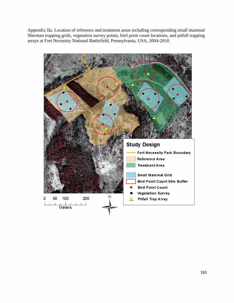
183

Appendix IIa. Location of reference and treatment areas including corresponding small mammal

Sherman trapping grids, vegetation survey points, bird point count locations, and pitfall trapping

arrays at Fort Necessity National Battlefield, Pennsylvania, USA, 2004-2010.

184

Appendix IIIa. Each pitfall array consisted of four 20 litter buckets placed in a triad and

connected with a 3-m long, 50-cm high silt fence. Six pitfall trap arrays, and 36 cover boards

were placed throughout the study area at Fort Necessity National Battlefield, Pennsylvania,

USA, 2004-2010.

185

Appendix IVa. Biotic community variables with non-significant F-tests, based on data collected

from Fort Necessity National Battlefield, Pennsylvania, USA, 2004-2010.

Pitfall Variables Year (df = 6,24) Plot Type (df = 1,4) Interaction (df = 6,24)

F-value p-value F-value p-value F-value p-value

White-footed mouse 1.22 0.332

0.29 0.621

1.22 0.332


2.95 0.161

0.42 0.858

Smoky shrew 2.12 0.009

1.09 0.356

0.26 0.948


4.00 0.116

0.94 0.487


0.67 0.458

1.97 0.111

Bog lemming 3.23 0.018

0.00 1.000

0.16 0.985

Species diversity (H‟) 3.49 0.013

0.00 0.973

1.09 0.399


0.33 0.597

1.07 0.408


0.11 0.760

1.17 0.357

Total relative abundance 2.39 0.059 1.58 0.278 0.42 0.860

Sherman Variables Year (df = 6,12) Plot Type (df = 1,2) Interaction (df = 6,12)



2.68 0.243

1.69 0.206


2.04 0.289

1.22 0.360

Woodland jumping mouse 3.52 0.030

0.20 0.698

0.42 0.850

Species diversity (H‟) 4.76 0.011

161.71 0.006

0.92 0.514


2.69 0.243

0.65 0.690

Species evenness (J) 3.02 0.049 20.47 0.046 0.90 0.524

Point-count Variables Year (df = 2,8) Plot Type (df = 1,4) Interaction (df = 2,8)


Early successional species 1.61 0.258

0.47 0.531

0.24 0.795

Generalist species 1.67 0.248

0.47 0.531

0.12 0.887


0.07 0.807

0.54 0.604

Eastern towhee 4.28 0.054

0.23 0.655

0.21 0.812

Field sparrow 2.47 0.147 1.45 0.295 1.96 0.203

Vegetation Variables Year (df = 2,19) Plot Type (df = 1,10) Interaction (df = 2,19)


Species Diversity (H‟) 4.47 0.026

9.50 0.012

2.26 0.131

Exotic species richness 5.79 0.011 8.20 0.017 1.50 0.248

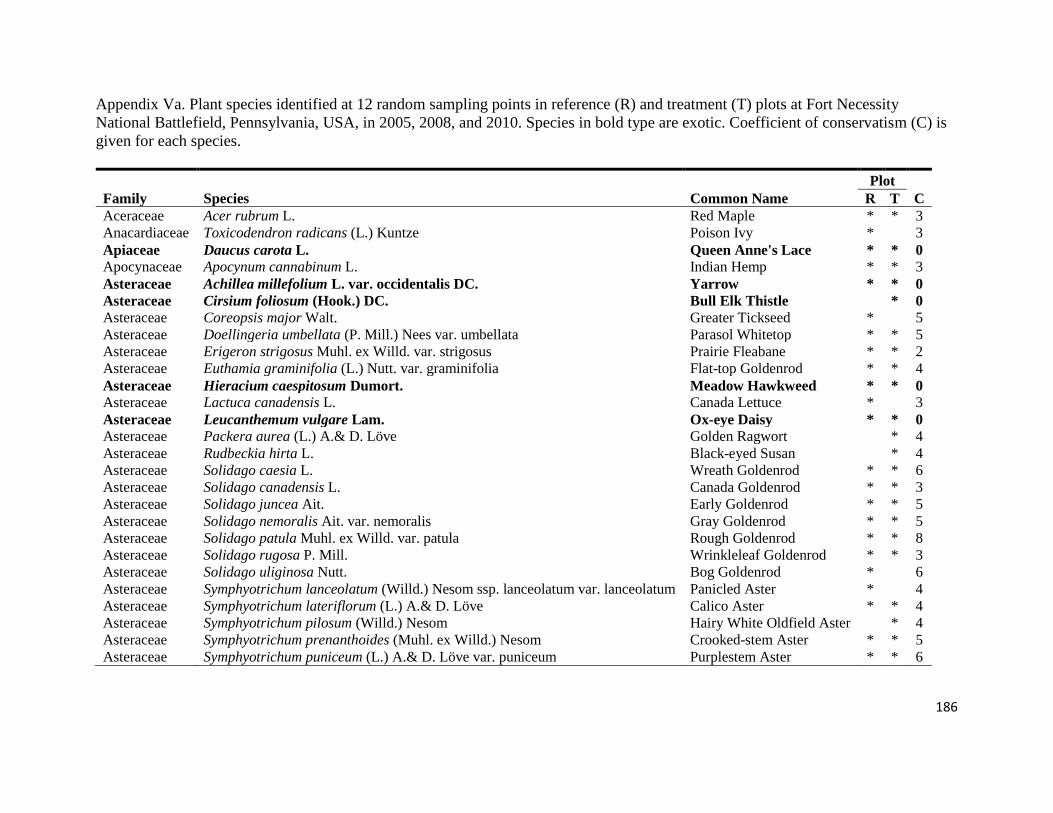
186

Appendix Va. Plant species identified at 12 random sampling points in reference (R) and treatment (T) plots at Fort Necessity

National Battlefield, Pennsylvania, USA, in 2005, 2008, and 2010. Species in bold type are exotic. Coefficient of conservatism (C) is

given for each species.

Plot

Family Species Common Name R T C

Aceraceae Acer rubrum L. Red Maple * * 3

Anacardiaceae Toxicodendron radicans (L.) Kuntze Poison Ivy *

3

Apiaceae Daucus carota L. Queen Anne's Lace * * 0

Apocynaceae Apocynum cannabinum L. Indian Hemp * * 3

Asteraceae Achillea millefolium L. var. occidentalis DC. Yarrow * * 0

Asteraceae Cirsium foliosum (Hook.) DC. Bull Elk Thistle

* 0

Asteraceae Coreopsis major Walt. Greater Tickseed *

5

Asteraceae Doellingeria umbellata (P. Mill.) Nees var. umbellata Parasol Whitetop * * 5

Asteraceae Erigeron strigosus Muhl. ex Willd. var. strigosus Prairie Fleabane * * 2

Asteraceae Euthamia graminifolia (L.) Nutt. var. graminifolia Flat-top Goldenrod * * 4

Asteraceae Hieracium caespitosum Dumort. Meadow Hawkweed * * 0

Asteraceae Lactuca canadensis L. Canada Lettuce *

3

Asteraceae Leucanthemum vulgare Lam. Ox-eye Daisy * * 0

Asteraceae Packera aurea (L.) A.& D. Löve Golden Ragwort

* 4

Asteraceae Rudbeckia hirta L. Black-eyed Susan

* 4

Asteraceae Solidago caesia L. Wreath Goldenrod * * 6

Asteraceae Solidago canadensis L. Canada Goldenrod * * 3

Asteraceae Solidago juncea Ait. Early Goldenrod * * 5

Asteraceae Solidago nemoralis Ait. var. nemoralis Gray Goldenrod * * 5

Asteraceae Solidago patula Muhl. ex Willd. var. patula Rough Goldenrod * * 8

Asteraceae Solidago rugosa P. Mill. Wrinkleleaf Goldenrod * * 3

Asteraceae Solidago uliginosa Nutt. Bog Goldenrod *

6

Asteraceae Symphyotrichum lanceolatum (Willd.) Nesom ssp. lanceolatum var. lanceolatum Panicled Aster *

4

Asteraceae Symphyotrichum lateriflorum (L.) A.& D. Löve Calico Aster * * 4

Asteraceae Symphyotrichum pilosum (Willd.) Nesom Hairy White Oldfield Aster

* 4

Asteraceae Symphyotrichum prenanthoides (Muhl. ex Willd.) Nesom Crooked-stem Aster * * 5

Asteraceae Symphyotrichum puniceum (L.) A.& D. Löve var. puniceum Purplestem Aster * * 6

187

Appendix Va. Continued

Asteraceae Taraxacum officinale G.H. Weber ex Wiggers ssp. officinale Common Dandelion

* 0

Asteraceae Vernonia gigantea (Walt.) Trel. ssp. gigantea Giant Ironweed * * 3

Campanulaceae Lobelia inflata L. Indian Tobacco

* 3

Caprifoliaceae Lonicera morrowii Gray Morrow's Honeysuckle * * 0

Caprifoliaceae Viburnum recognitum Fern. Southern Arrowwood * * 6

Caryophyllaceae Cerastium fontanum Baumg. ssp. vulgare (Hartman) Greuter & Burdet Common Mouse-ear Chickweed * * 0

Caryophyllaceae Cerastium nutans Raf. var. nutans Powderhorn Chickweed

* 4

Caryophyllaceae Dianthus armeria L. Deptford Pink

* 0

Caryophyllaceae Stellaria longifolia Muhl. ex Willd. var. longifolia Longleaf Starwort * * 6

Clusiaceae Hypericum perforatum L. Common St. John's Wort

* 0

Clusiaceae Hypericum punctatum Lam. Spotted St. John's Wort *

4

Convolvulaceae Calystegia sepium (L.) R. Br. ssp. sepium Hedge False Bindweed

* 0

Cornaceae Cornus racemosa Lam. Gray Dogwood

* 6

Cyperaceae Carex digitalis Willd. Slender Woodland Sedge

* 4

Cyperaceae Carex hirsutella Mackenzie Fuzzy Wuzzy Sedge * * 4

Cyperaceae Carex virescens Muhl. ex Willd. Ribbed Sedge *

6

Dryopteridaceae Dryopteris carthusiana (Vill.) H.P. Fuchs Spinulose Woodfern

* 6

Eleagnaceae Eleagnus umbellata Thunb. Var. parvifolia (Royle) Schneid. Autumn olive

* 0

Euphorbiaceae Euphorbia corollata L. Flowering Spurge *

5

Fabaceae Amphicarpaea bracteata (L.) Fern. Hog Peanut

* 4

Fabaceae Coronilla varia L. Crown Vetch *

0

Fabaceae Melilotus officinalis (L.) Lam. Yellow Sweet Clover

* 0

Fabaceae Robinia pseudoacacia L. Black Locust

* 2

Fabaceae Trifolium aureum Pollich Golden Clover * * 0

Fabaceae Trifolium pratense L. Red Clover

* 0

Fabaceae Trifolium repens L. Sweet White Clover * * 0

Fabaceae Trifolium spp. Clover spp.

* 0

Fagaceae Quercus rubra L. Red Oak * * 5

Fagaceae Quercus spp. Oak spp. *

0

Iridaceae Sisyrinchium angustifolium P. Mill. Narrowleaf Blue-eyed Grass * 4

188


Lamiaceae Clinopodium vulgare L. Wild Basil * * 2

Lamiaceae Lycopus virginicus L. Bugleweed * * 4

Lamiaceae Prunella vulgaris L. Common Self-heal * * 1

Lamiaceae Pycnanthemum incanum (L.) Michx. Hoary Mountain Mint * * 6

Liliaceae Medeola virginiana L. Indian Cucumber *

6

Lycopodiaceae Lycopodium digitatum Dill. ex A. Braun Fan Clubmoss * * 4

Magnoliaceae Liriodendron tulipifera L. Tulip Poplar *

5

Magnoliaceae Magnolia acuminata (L.) L. Cucumber Magnolia *

6

Oleaceae Fraxinus americana L. White Ash * * 6

Onagraceae Oenothera perennis L. Little Evening Primrose

* 5

Ophioglossaceae Botrychium dissectum Spreng. Cutleaf Grapefern * * 4

Orchidaceae Liparis liliifolia (L.) Rich. ex Ker Gawl. Brown Widelip Orchid

* 5

Oxalidaceae Oxalis stricta L. Yellow Woodsorrel * * 2

Pinaceae Pinus strobus L. White Pine

* 5

Plantaginaceae Plantago lanceolata L. Narrowleaf Plantain * * 0

Plantaginaceae Plantago major L. Wide Leaf Plantain

* 0

Poaceae Agrostis gigantea Roth Redtop Grass * * 0

Poaceae Agrostis perennans (Walt.) Tuckerman Upland Bentgrass * * 4

Poaceae Andropogon virginicus L. var. virginicus Broomsedge Bluestem * * 3

Poaceae Anthoxanthum odoratum L. ssp. odoratum Sweet Vernal Grass * * 0

Poaceae Arrhenatherum elatius (L.) Beauv. Ex J.& K. Presl Tall Oat Grass * * 0

Poaceae Bromus inermis Leyss. ssp. inermis var. inermis Smooth Brome

* 0

Poaceae Dactylis glomerata L. ssp. glomerata Orchard Grass * * 0

Poaceae Danthonia compressa Austin ex Peck Flattened Oatgrass * * 6

Poaceae Danthonia spicata (L.) Beauv. ex Roemer & J.A. Schultes Poverty Grass * * 5

Poaceae Dichanthelium clandestinum (L.) Gould Deer-tongue Grass * * 3

Poaceae Dichanthelium scabriusculum (Elliot) Gould & C.A. Clark Wooly Rosette Grass * * 9

Poaceae Dichanthelium sphaerocarpon (Ell.) Gould Roundseed Panicgrass

* 4

Poaceae Dichanthelium spp. Panic Grass * * 0

Poaceae Elyleymus spp. Wild Rye *

0

Poaceae Holcus lanatus L. Velvet Grass * * 0

Poaceae Lolium arundinaceum (Schreb.) S.J. Darbyshire Tall Fescue

* 0

Poaceae Lolium perenne L. ssp. perenne Perennial Ryegrass * 0

189


Poaceae Danthonia spp. Oat Grass * * 0

Poaceae Phleum pratense L. Timothy Grass

* 0

Poaceae Poa trivialis L. Rough Bluegrass * * 0

Polygonaceae Rumex acetosella L. Sheep Sorrel * * 0

Primulaceae Lysimachia lanceolata Walt. Lance-leafed Loostrife * * 6

Ranunculaceae Ranunculus spp. Ranunculus spp. * * 0

Rosaceae Amelanchier arborea (Michx. f.) Fern. var. arborea Common Serviceberry * * 5

Rosaceae Crataegus pruinosa (Wendl. f.) K. Koch Waxyfruit Hawthorne * * 5

Rosaceae Fragaria virginiana Duchesne ssp. virginiana Wild Strawberry * * 3

Rosaceae Malus coronaria (L.) P. Mill. var. coronaria Sweet Crabapple * * 3

Rosaceae Potentilla simplex Michx. Common Cinquefoil * * 4

Rosaceae Prunus serotina Ehrh. var. serotina Black Cherry * * 4

Rosaceae Rosa multiflora Thunb. ex Murr. Multiflora Rose

* 0

Rosaceae Rubus flagellaris Willd. Northern Dewberry * * 5

Rosaceae Rubus hispidus L. Bristly Dewberry * * 5

Rosaceae Rubus spp. Rubus * * 0

Rubiaceae Galium circaezans Michx. Licorice Bedstraw *

6

Scrophulariaceae Veronica officinalis L. Common Gypsyweed * * 0

Scrophulariaceae Veronica serpyllifolia L. ssp. serpyllifolia Thymeleaf Speedwell * * 0

Smilacaceae Smilax glauca Walt. Cat Greenbrier *

5

Smilacaceae Smilax rotundifolia L. Common Greenbriar

* 4

Solanaceae Solanum carolinense L. var. carolinense Carolina Horsenettle * * 3

Violaceae Viola blanda Willd. Sweet White Violet *

5

Violaceae Viola sororia Willd. Common Blue Violet * * 4

Violaceae Viola spp Viola spp. * * 0

Vitaceae Parthenocissus quinquefolia (L.) Planch. Virginia Creeper *

4

Vitaceae Vitis aestivalis Michx. Summer Grape * 5

190

Appendix VIa. The most common shrub species identified, based on percent plot coverage, across Fort Necessity National Battlefield,

Pennsylvania, USA, from 2005, 2008, and 2010 averaged. Any species with a total cover of 5% and greater were included in the table.

Species in bold are exotic.

Family Scientific name Common name Total cover Reference Treatment

Caprifoliaceae Lonicera morrowii Gray Morrow's honeysuckle 56.46 74.53 38.38

Rosaceae Malus coronaria (L.) P. Mill. var. coronaria Sweet crabapple 11.41 12.50 10.31

Rosaceae Prunus serotina Ehrh. var. serotina Black cherry 8.33 14.17 2.50

Magnoliaceae Magnolia acuminata (L.) L. Cucumber magnolia 7.50 15.00 0.00

Fabaceae Robinia pseudoacacia L. Black locust 7.08 0.00 14.17

Caprifoliaceae Viburnum dentatum L. var. dentatum Southern arrowwood 5.83 2.50 9.17

191

Appendix VIIa. Mean ( ) and SE of floristic metrics measured at reference and treatment plots at Fort Necessity National Battlefield,

Pennsylvania, USA, during 2005, 2008, and 2010. *Post-removal surveys took place following removal procedures.

Lonicera

morrowii Percent

cover

Native Shrub

Percent Cover

Shrub Species

Richness

Exotic Species

Richness

Shannon-Wiener

Diversity Index

(H') - Herbs &

Shrubs

n SE SE SE SE SE

Reference

2005 6 63.75 13.05

0.42 0.42

1.17 0.17

4.50 0.76

2.25 0.21

2008 5 68.50 18.28

17.50 5.97

4.80 0.37

4.40 0.40

2.41 0.15

2010 6 65.83 11.12

12.92 6.72

3.00 0.58

3.33 0.33

1.94 0.09

Overall 17 65.88 7.56

9.85 3.20

2.88 0.43

4.06 0.33

2.18 0.10

Treatment

2005 6 69.58 7.84

19.17 7.60

2.50 0.43

6.50 0.61

2.65 0.09

*2008 6 30.83 10.01

9.59 4.63

3.33 0.88

4.67 0.33

2.68 0.08

*2010 6 8.33 3.00

10.83 5.73

2.67 0.99

4.33 0.21

2.60 0.11

Overall 17 36.25 7.37 13.19 3.47 2.83 0.44 5.17 0.33 2.64 0.05

192

Appendix VIIa. Continued

Species Richness

(S) Herbs &

Shrubs

Species

Evenness (J) -

Herbs &

Shrubs

Mean Coefficient

of Conservatism

(C)

Mean Floristic

Quality Index

(FQI)

n SE SE SE SE

Reference

2005 6 23.33 1.69

0.71 0.05

3.84 0.09

10.59 0.57

2008 5 24.40 2.32

0.76 0.04

2.74 0.19

6.92 0.63

2010 6 19.50 1.02

0.65 0.02

4.36 0.14

9.85 0.46

Overall 17 22.29 1.05

0.70 0.02

3.70 0.18

9.25 0.48

Treatment

2005 6 32.67 1.94

0.76 0.02

3.80 0.14

11.30 0.86

*2008 6 24.33 1.74

0.84 0.02

2.44 0.14

5.46 0.51

*2010 6 19.33 1.87

0.88 0.02

3.40 0.30

6.99 1.05

Overall 17 25.44 1.67 0.83 0.02 3.21 0.18 7.90 0.75

193

Appendix VIIIa. The most common herbaceous species identified, based on percent plot coverage, across Fort Necessity National

Battlefield, Pennsylvania, USA, from 2005, 2008, and 2010 averaged. Any species with a total cover of 5% and greater were included

in the table. Species in bold are exotic.

Family Scientific name Common name Total cover Reference Treatment

Poaceae Agrostis gigantea Roth Redtop grass 11.53 12.68 10.39

Poaceae Danthonia compressa Austin ex Peck Flattened oatgrass 11.46 2.50 20.42

Asteraceae Solidago rugosa P. Mill. Wrinkle-leaf goldenrod 11.45 13.87 9.04

Asteraceae Solidago juncea Ait. Early goldenrod 9.64 12.10 7.19

Asteraceae Vernonia gigantea (Walt.) Trel. ssp. gigantea Giant ironweed 8.75 2.50 15.00

Asteraceae Solidago patula Muhl. ex Willd. var. patula Rough-leaved goldenrod 8.44 7.71 9.17

Convolvulaceae Calystegia sepium (L.) R. Br. ssp. sepium Hedge false bindweed 7.50 0.00 15.00

Lycopodiaceae Lycopodium digitatum Dill. ex A. Braun Fan clubmoss 7.25 5.00 9.50

Rosaceae Rubus flagellaris Willd. Northern dewberry 7.03 7.40 6.67

Poaceae Dactylis glomerata L. ssp. glomerata Orchard grass 6.48 4.29 8.68

Asteraceae Solidago canadensis L. Canada goldenrod 6.43 7.86 5.00

Poaceae Anthoxanthum odoratum L. ssp. odoratum Sweet vernal grass 6.06 4.84 7.28

Asteraceae Achillea millefolium L. var. occidentalis DC. Yarrow 5.71 4.20 7.22

Poaceae Holcus lanatus L. Common velvet grass 5.51 3.04 7.98

Asteraceae Leucanthemum vulgare Lam. Ox-eye daisy 5.27 2.50 8.03

Lamiaceae Clinopodium vulgare L. Wild basil 5.21 4.35 6.07

194

Appendix IXa: Overall mean ( ) and SE of male American woodcock for the overall reference

and treatment areas at Fort Necessity National Battlefield, Pennsylvania, USA. We performed

singing ground surveys from 2004 throughout 2010 during the winter and spring breeding

months (February – May). *Post-removal surveys took place following the implementation of

management procedures designed to remove Morrow‟s honeysuckle.

Total No. Males Highest No. of Males Overall No. Males Heard Calling

n Heard Calling/Year Heard Calling/Survey SE

Reference

2004 8 6 2 0.75 0.25

2005 8 10 3 1.26 0.45

2006 6 1 1 0.18 0.17

2007 9 14 6 1.56 0.78

2008 8 7 3 0.87 0.40

2009 7 9 4 1.29 0.61

2010 15 30 5 2.01 0.40

Overall 61 77 6 1.27 0.15

Treatment

2004 8 14 3 1.76 0.31

2005 8 14 3 1.76 0.41

2006 6 16 7 2.66 1.02

*2007 9 30 7 3.32 0.94

*2008 8 18 5 2.26 0.49

*2009 7 5 2 0.72 0.29

*2010 15 45 5 3.00 0.26

Overall 61 142 7 2.33 0.19

195

Appendix Xa: Mean ( ) and SE of male American woodcock for individual reference and

treatment plots at Fort Necessity National Battlefield. We performed singing ground surveys

from 2004 throughout 2010 during the winter and spring breeding months (February – May).

*Post-removal surveys took place following the implementation of management procedures

designed to remove Morrow‟s honeysuckle.

No. Males Heard Calling/Sample Plot

n SE

Reference

2004 24 0.25 0.11

2005 24 0.42 0.12

2006 18 0.06 0.06

2007 27 0.52 0.17

2008 24 0.29 0.13

2009 21 0.43 0.15

2010 45 0.67 0.13

Overall 183 0.42 0.05

Treatment

2004 16 0.88 0.18

2005 16 0.88 0.18

2006 12 1.33 0.40

*2007 18 1.66 0.36

*2008 16 1.13 0.20

*2009 14 0.36 0.13

*2010 30 1.50 0.14

Overall 122 1.17 0.09

196

Appendix XIa: Mapped locations of male American woodcock heard calling in reference and




of males/survey day.

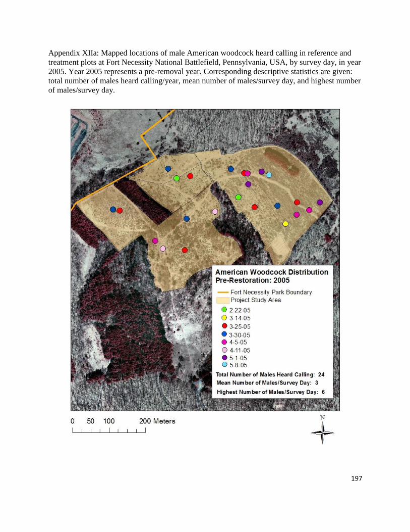
197

Appendix XIIa: Mapped locations of male American woodcock heard calling in reference and





198

Appendix XIIIa: Mapped locations of male American woodcock heard calling in reference and





199

Appendix XIVa: Mapped locations of male American woodcock heard calling in reference and





200

Appendix XVa: Mapped locations of male American woodcock heard calling in reference and





201

Appendix XVIa: Mapped locations of male American woodcock heard calling in reference and





202

Appendix XVIIa: Mapped locations of male American woodcock heard calling in reference and





203

Appendix XVIIIa: Species of songbirds and their associated habitat guilds observed at Fort

Necessity National Battlefield, Pennsylvania, USA, during 2004, 2008, and 2010 point counts

surveys.

Family Scientific Name Species Code Species

Early-Successional Habitat Guild

Cardinalidae Cardinalis cardinalis Northern Cardinal NOCA

Cardinalidae Passerina cyanea Indigo Bunting INBU

Emberizidae Melospiza melodia Song Sparrow SOSP

Emberizidae Pipilo erythrophthalmus Eastern Towhee ETOW

Emberizidae Spizella pusilla Field Sparrow FISP

Fringillidae Carduelis tristis American Goldfinch AMGO

Hirundinidae Hirundo rustica Barn Swallow BARS

Icteridae Quiscalus quiscula Common Grackle COGR

Mimidae Dumetella carolinensis Grey Catbird GRCA

Mimidae Mimus polyglottos Northern Mockingbird NOMO

Mimidae Toxostoma rufum Brown Thrasher BRTH

Parulidae Dendroica discolor Prairie Warbler PRAW

Parulidae Dendroica pensylvanica Chestnut-sided Warbler CSWA

Parulidae Geothlypis trichas Common Yellowthroat COYE

Parulidae Vermivora chrysoptera Golden-winged Warbler GWWA

Tyrannidae Sayornis phoebe Eastern Phoebe EAPH

Vireonidae Vireo griseus White-eyed Vireo WEVI

Generalist Habitat Guild

Bombycillidae Bombycilla cedrorum Cedar Waxwing CEDW

Cardinalidae Pheucticus ludovicianus Rose-breasted Grosbeak RBGR

Corvidae Corvus brachyrhynchos American Crow AMCR

Corvidae Corvus corax Common Raven CORA

Cuculidae Coccyzus americanus Yellow-billed Cuckoo YBCU

Emberizidae Spizella passerina Chipping Sparrow CHSP

204

Appendix XVIIIa. Continued

Family Scientific Name Species Code Species

Generalist Habitat Guild

Paridae Baeolophus bicolor Tufted Titmouse ETTI

Paridae Poecile atricapilla Black-capped Chickadee BCCH

Parulidae Parula americana Northern Parula NOPA

Parulidae Wilsonia citrina Hooded Warbler HOWA

Picidae Colaptes auratus Northern Flicker NOFL

Picidae Picoides pubescens Downy Woodpecker DOWO

Trochilidae Archilochus colubris Ruby-throated Hummingbird RTHU

Vireonidae Vireo olivaceus Red-eyed Vireo REVI

Late-Successional Habitat Guild

Cardinalidae Piranga olivacea Scarlet Tananger SCTA

Parulidae Dendroica virens Black-throated Green Warbler BTGW

Picidae Dryocopus pileatus Pileated Woodpecker PIWO

205

Appendix XIXa: Total songbird species observations during point count surveys at Fort Necessity National Battlefield, Pennsylvania,

USA, during 2004, 2008, and 2010. Observations are categorized based on plot type and timing of restoration (Pre-T, Post-T, Pre-R,

Post-R). Code is as follows: T=treatment, R=Reference, Pre = 2004, Post = 2008, 2010.

0

5

10

15

20

25

30

Ced

ar W

axw

ing

North

ern

Card

ina

l

Ind

igo

Bu

ntin

g

Rose

-Bre

aste

d G

rosb

ea

k

Sca

rlet T

an

age

r

Am

eric

an

Cro

w

Com

mo

n R

ave

n

Ye

llow

-Bille

d C

ucko

o

So

ng S

pa

rrow

Ea

ste

rn T

ow

he

e

Chip

pin

g S

pa

rrow

Fie

ld S

pa

rrow

Am

eric

an

Go

ldfin

ch

Ba

rn S

wa

llow

Com

mo

n G

rackle

Gra

y C

atb

ird

North

ern

Mo

ckin

gb

ird

Bro

wn

Th

rash

er

Tu

fted

Titm

ou

se

Bla

ck-C

ap

pe

d C

hic

ka

de

e

Pra

irie W

arb

ler

Che

stn

ut-S

ide

d W

arb

ler

Bla

ck-T

hro

ate

d G

ree

n

Com

mo

n Y

ello

wth

roa

t

North

ern

Pa

rula

Go

lde

n-W

inge

d W

arb

ler

Hoo

de

d W

arb

ler

North

ern

Flic

ke

r

Pile

ate

d W

oo

dpe

cke

r

Dow

ny W

ood

pecke

r

Rub

y-T

hro

ate

d …

Ea

ste

rn P

ho

eb

e

Wh

ite-E

ye

d V

ireo

Red

-Eye

d V

ireo

N

um

be

r o

f O

bse

rva

tio

n

Pre-Treatment

Post-Treatment

Pre-Reference

Post-Reference

Fort Necessity Restoration Project Pre/Post Treatment Songbird Point Count Observations

35 Species Recorded 388 Identified Individuals

206

Appendix XXa: Mean ( ) and SE of songbird metrics measured at reference and treatment point count locations at Fort Necessity

National Battlefield, Pennsylvania, USA. We performed point count surveys during the 2004, 2008, and 2010 breeding period.

Numbers of observations of the 2 most common species captured are listed using the following species codes: Eastern towhee

(EATO), and Field sparrow (FISP). *Post removal surveys took place following the implementation of management procedures

designed to remove Morrow‟s honeysuckle.

Proportion of

Early

Successional

species

Proportion

of

Generalist

Species

Shannon-

Wiener

Diversity

Index (H')

Species

Richness (S)

Species

Evenness

(J)

EATO

Observations

(per 5 minute

count)

FISP

Observations

(per 5 minute

count)

n SE SE SE SE SE SE SE

Reference

2004 6 0.92 0.04

0.08 0.04

1.62 0.07

5.67 0.49

0.94 0.13

1.33 0.61

1.17 0.54

2008 3 0.80 0.10

0.20 0.20

2.11 0.07

9.33 0.88

0.95 0.01

2.33 0.88

1.00 0.00

2010 6 0.78 0.06

0.21 0.05

2.18 0.08

10.00 0.73

0.95 0.01

2.17 0.54

1.33 0.56

Overall 15 0.84 0.04

0.16 0.03

1.94 0.08

8.13 0.65

0.95 0.01

1.87 0.36

1.20 0.30

Treatment

2004 6 0.83 0.09

0.15 0.10

1.65 0.14

6.17 0.87

0.94 0.02

0.67 0.33

0.83 0.31

*2008 3 0.77 0.02

0.23 0.02

2.08 0.09

8.67 0.88

0.97 0.01

2.33 0.33

2.33 0.33

*2010 6 0.77 0.04

0.22 0.03

2.07 0.14

9.50 0.85

0.92 0.04

1.83 0.48

3.33 1.17

Overall 15 0.79 0.04 0.20 0.04 1.90 0.10 8.00 0.63 0.94 0.02 1.47 0.29 2.13 0.55

207

Appendix XXIa: Total small mammal species captures during Sherman trapping at Fort Necessity National Battlefield, Pennsylvania,

USA, from 2004 – 2010. Observations are categorized based on plot type and timing of restoration (Pre-T, Post-T, Pre-R, Post-R).

Code is as follows: T=treatment, R=Reference, Pre = 2005, Post = 2008, 2010.

0

25

50

75

100

125

150

175

200

225

250

275

300

325

Woo

dla

nd

Ju

mp

ing

Mo

use

Me

ad

ow

Ju

mp

ing M

ou

se

Me

ad

ow

Vo

le

Wh

ite-F

oote

d M

ou

se

Dee

r Mo

use

S. B

og L

em

min

g

S. F

lyin

g S

qu

irrel

E. C

hip

mu

nk

N. S

ho

rt-Ta

iled

Sh

rew

Ma

ske

d S

hre

w

Sm

oky S

hre

w

Nu

mb

er

of

Ca

ptu

res

Pre-Treatment

Pre-Reference

Post-Treatment

Post-Reference

Total Pre/Post Fort Necessity Restoration Project Small Mammal Sherman Trap Captures

38,827 Trap Nights 11 Species Recorded

1,445 Distinct Captures

208

Appendix XXIIa: List of mammal species and their associated observation method at Fort Necessity National Battlefield,

Pennsylvania, USA, 2004 – 2010.

Family Scientific Name Species Species Code Observation Method

Canidae Red Fox Vulpes vulpes VUVU Observation In Study Plot

Didelphidae Virginia Opossum Didelphis virginianus DIVI Pitfall/Tomahawk

Dipodidae Meadow Jumping Mouse Zapus hudsonius ZAHU Pitfall/Sherman

Dipodidae Woodland Jumping Mouse Napaeozapus insignis NAIN Pitfall/Sherman

Muridae Deer Mouse Peromyscus maniculatus PEME Pitfall/Sherman

Muridae Meadow Vole Microtus pennsylvanicus MIPE Pitfall/Sherman

Muridae Pine Vole Microtus pinetorum MIPI Sherman

Muridae Southern Bog Lemming Synaptomys cooperi SYCO Pitfall/Sherman

Muridae White-footed Mouse Peromyscus leucopus PELE Pitfall/Sherman

Procyonidae Raccoon Procyon lotor PRLO Tomahawk

Sciuridae Eastern Chipmonk Tamias striatus TAST Sherman

Sciuridae Southern Flying Squirrel Glaucomys volans GLVO Sherman

Soricidae Masked Shrew Sorex cinereus SOCI Pitfall/Sherman

Soricidae Short-tailed Shrew Blarina brevicauda BLBR Pitfall/Sherman

Soricidae Smoky Shrew Sorex fumeus SOFU Pitfall/Sherman

Talpidae Hairy-tail Mole Parascalops breweri PABR Observation In Study Plot

Talpidae Star-nosed Mole Condylura cristata COCR Observation In Study Plot

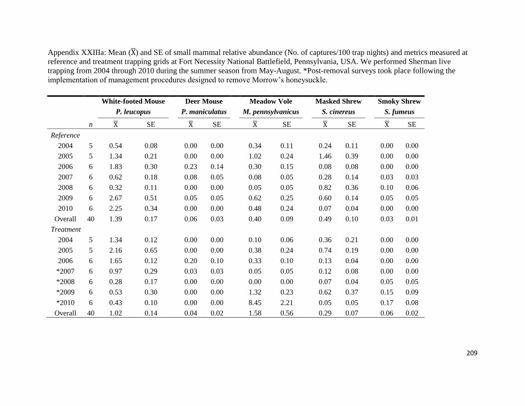
209

Appendix XXIIIa: Mean ( ) and SE of small mammal relative abundance (No. of captures/100 trap nights) and metrics measured at

reference and treatment trapping grids at Fort Necessity National Battlefield, Pennsylvania, USA. We performed Sherman live

trapping from 2004 through 2010 during the summer season from May-August. *Post-removal surveys took place following the

implementation of management procedures designed to remove Morrow‟s honeysuckle.

White-footed Mouse Deer Mouse Meadow Vole Masked Shrew Smoky Shrew

P. leucopus P. maniculatus M. pennsylvanicus S. cinereus S. fumeus

n SE SE SE SE SE

Reference

2004 5 0.54 0.08

0.00 0.00

0.34 0.11

0.24 0.11

0.00 0.00

2005 5 1.34 0.21

0.00 0.00

1.02 0.24

1.46 0.39

0.00 0.00

2006 6 1.83 0.30

0.23 0.14

0.30 0.15

0.08 0.08

0.00 0.00

2007 6 0.62 0.18

0.08 0.05

0.08 0.05

0.28 0.14

0.03 0.03

2008 6 0.32 0.11

0.00 0.00

0.05 0.05

0.82 0.36

0.10 0.06

2009 6 2.67 0.51

0.05 0.05

0.62 0.25

0.60 0.14

0.05 0.05

2010 6 2.25 0.34

0.00 0.00

0.48 0.24

0.07 0.04

0.00 0.00

Overall 40 1.39 0.17

0.06 0.03

0.40 0.09

0.49 0.10

0.03 0.01

Treatment

2004 5 1.34 0.12

0.00 0.00

0.10 0.06

0.36 0.21

0.00 0.00

2005 5 2.16 0.65

0.00 0.00

0.38 0.24

0.74 0.19

0.00 0.00

2006 6 1.65 0.12

0.20 0.10

0.33 0.10

0.13 0.04

0.00 0.00

*2007 6 0.97 0.29

0.03 0.03

0.05 0.05

0.12 0.08

0.00 0.00

*2008 6 0.28 0.17

0.00 0.00

0.00 0.00

0.07 0.04

0.05 0.05

*2009 6 0.53 0.30

0.00 0.00

1.32 0.23

0.62 0.37

0.15 0.09

*2010 6 0.43 0.10

0.00 0.00

8.45 2.21

0.05 0.05

0.17 0.08

Overall 40 1.02 0.14 0.04 0.02 1.58 0.56 0.29 0.07 0.06 0.02

210

Appendix XXIIIa. Continued

Short-tailed Shrew Meadow Jumping Mouse

Woodland Jumping Mouse

Eastern Chipmunk

B. brevicauda Z. hudsonius

N. insignis

T. striatus

n SE SE SE SE

Reference

2004 5 0.62 0.28

1.64 0.83

0.00 0.00

0.00 0.00

2005 5 0.38 0.24

1.02 0.29

0.30 0.18

0.13 0.08

2006 6 0.28 0.10

0.08 0.05

0.00 0.00

0.00 0.00

2007 6 0.18 0.09

0.05 0.05

0.00 0.00

0.15 0.10

2008 6 0.93 0.33

0.05 0.05

0.00 0.00

0.03 0.03

2009 6 0.88 0.39

0.22 0.22

0.20 0.16

0.00 0.00

2010 6 0.53 0.14

0.03 0.03

0.17 0.11

0.03 0.03

Overall 40 0.55 0.10

0.40 0.14

0.09 0.04

0.05 0.02

Treatment

2004 5 0.54 0.23

0.70 0.36

0.00 0.00

0.00 0.00

2005 5 0.78 0.30

1.12 0.20

0.34 0.21

0.00 0.00

2006 6 0.60 0.28

0.08 0.05

0.00 0.00

0.00 0.00

*2007 6 0.07 0.04

0.20 0.09

0.03 0.03

0.00 0.00

*2008 6 0.37 0.22

0.03 0.03

0.00 0.00

0.04 0.04

*2009 6 0.43 0.16

0.03 0.03

0.08 0.08

0.00 0.00

*2010 6 0.33 0.16

0.15 0.07

0.00 0.00

0.00 0.00

Overall 40 0.44 0.08 0.30 0.08 0.06 0.03 0.01 0.01

211


Southern Flying Squirrel

Southern Bog Lemming

Shannon-Wiener Index

Species Richness

G. volans

S. cooperi

H'

S

n SE SE SE SE

Reference

2004 5 0.00 0.00

0.00 0.00

1.05 0.12

3.50 0.65

2005 5 0.00 0.00

0.04 0.04

1.52 0.12

5.25 0.75

2006 6 0.00 0.00

0.00 0.00

0.86 0.07

3.20 0.37

2007 6 0.00 0.00

0.00 0.00

0.98 0.10

3.20 0.31

2008 6 0.00 0.00

0.00 0.00

0.84 0.20

0.20 0.63

2009 6 0.00 0.00

0.00 0.00

1.08 0.17

4.33 0.84

2010 6 0.00 0.00

0.00 0.00

0.91 0.17

3.67 0.42

Overall 40 0.00 0.00

0.01 0.01

1.02 0.06

3.75 0.23

Treatment

2004 5 0.00 0.00

0.00 0.00

1.00 0.23

2.67 0.67

2005 5 0.00 0.00

0.00 0.00

1.35 0.08

5.33 0.33

2006 6 0.10 0.10

0.00 0.00

1.08 0.12

4.00 0.71

*2007 6 0.00 0.00

0.00 0.00

0.75 0.22

3.00 0.58

*2008 6 0.00 0.00

0.00 0.00

0.47 0.17

2.20 0.37

*2009 6 0.00 0.00

0.03 0.03

1.07 0.16

4.00 0.68

*2010 6 0.00 0.00

0.00 0.00

0.54 0.13

3.40 0.60

Overall 40 0.01 0.01 0.01 0.01 0.88 0.07 3.58 0.23

212


Species Evenness

Total Relative

J

Abundance

n SE SE

Reference

2004 5 0.85 0.07

3.44 0.99

2005 5 0.91 0.02

5.76 0.93

2006 6 0.78 0.04

2.80 0.41

2007 6 0.87 0.03

1.47 0.22

2008 6 0.74 0.15

2.20 0.71

2009 6 0.78 0.03

5.27 1.05

2010 6 0.69 0.07

3.57 0.18

Overall 40 0.80 0.03

3.45 0.33

Treatment

2004 5 0.80 0.08

3.06 0.84

2005 5 0.84 0.02

5.64 0.88

2006 6 0.77 0.04

3.12 0.39

*2007 6 0.66 0.16

1.43 0.27

*2008 6 0.52 0.18

0.85 0.27

*2009 6 0.81 0.03

3.20 0.92

*2010 6 0.41 0.07

9.65 2.12

Overall 40 0.68 0.04 3.83 0.57

213

Appendix XXIVa: Total small mammal species captures during pitfall arrays at Fort Necessity National Battlefield, Pennsylvania,

USA, from 2004 – 2010. Observations are categorized based on plot type and timing of restoration (Pre-T, Post-T, Pre-R, Post-R).

Code is as follows: T=treatment, R=Reference, Pre = 2005, Post = 2008, 2010.

0

10

20

30

40

50

60

Virg

inia

Op

ossu

m

Me

ad

ow

Ju

mp

ing

Mo

use

Woo

dla

nd

Ju

mp

ing

Mo

use

Me

ad

ow

Vo

le

Wh

ite-F

oote

d M

ou

se

Dee

r Mo

use

S. B

og L

em

min

g

N. S

ho

rt-Ta

iled

S

hre

w

Ma

ske

d S

hre

w

Sm

oky S

hre

w

Nu

mb

er

of

Ca

ptu

res

Pre-Treatment

Pre-Reference

Post-Treatment

Post-Reference

Small Mammal Pitfall Trap Captures

504 Trap Nights 10 Species Recorded 349 Distinct Captures

214

Appendix XXVa: Mean ( ) and SE of small mammal relative abundance (No. of captures/100 trap nights) and metrics measured at

reference and treatment pitfall arrays at Fort Necessity National Battlefield, Pennsylvania, USA. We trapped using the pitfall arrays

from 2004 through 2010 during the summer season from May-August. *Post-removal surveys took place following the

implementation of management procedures designed to remove Morrow‟s honeysuckle.

White-footed Mouse

Deer Mouse

Meadow Vole

Masked Shrew

Smoky Shrew

P. leucopus

P. maniculatus

M. pennsylvanicus

S. cinereus

S. fumeus

n SE SE SE SE SE

Reference

2004 9 0.00 0.00

0.00 0.00

2.78 2.78

50.00 12.50

2.78 2.78

2005 9 0.00 0.00

0.00 0.00

2.78 2.78

27.78 10.58

11.11 6.05

2006 9 2.78 2.78

2.78 2.78

0.00 0.00

16.67 7.22

0.00 0.00

2007 9 0.00 0.00

0.00 0.00

0.00 0.00

25.00 11.78

11.11 6.05

2008 9 5.56 5.56

0.00 0.00

2.78 2.78

36.11 14.50

11.11 11.11

2009 9 2.78 2.78

0.00 0.00

11.11 8.45

63.89 26.72

27.78 12.11

2010 9 2.78 2.78

0.00 0.00

5.56 3.67

8.33 5.89

8.33 8.33

Overall 63 1.98 1.03

0.40 0.40

3.57 1.48

32.54 5.60

10.32 2.97

Treatment

2004 9 0.00 0.00

0.00 0.00

0.00 0.00

47.22 15.28

2.78 2.78

2005 9 0.00 0.00

0.00 0.00

2.78 2.78

41.67 21.25

2.78 2.78

2006 9 0.00 0.00

0.00 0.00

2.78 2.78

63.89 13.89

0.00 0.00

*2007 9 8.33 4.17

0.00 0.00

5.56 3.67

38.89 11.87

2.78 2.78

*2008 9 2.78 2.78

0.00 0.00

0.00 0.00

61.11 27.67

11.11 8.45

*2009 9 0.00 0.00

0.00 0.00

25.00 9.32

72.22 26.82

16.67 11.02

*2010 9 8.33 5.89

0.00 0.00

27.78 10.58

27.78 13.47

8.33 5.89

Overall 63 2.78 1.15 0.00 0.00 9.13 2.49 50.40 7.28 6.35 2.26

215

Appendix XXVa. Continued

Short-tailed Shrew

Meadow Jumping Mouse

Woodland Jumping Mouse

Southern Bog Lemming

B. brevicauda

Z. hudsonius

N. insignis

S.cooperi

n SE SE SE SE

Reference

2004 9 2.78 2.78

2.78 2.78

0.00 0.00

0.00 0.00

2005 9 13.89 7.35

2.78 2.78

0.00 0.00

0.00 0.00

2006 9 2.78 2.78

0.00 0.00

0.00 0.00

0.00 0.00

2007 9 0.00 0.00

0.00 0.00

0.00 0.00

0.00 0.00

2008 9 8.33 5.89

5.56 3.67

0.00 0.00

2.78 2.78

2009 9 0.00 0.00

11.11 7.35

2.78 2.78

8.33 5.89

2010 9 11.11 8.45

0.00 0.00

0.00 0.00

0.00 0.00

Overall 63 5.56 1.91

3.17 1.33

0.40 0.40

1.59 0.96

Treatment

2004 9 2.78 2.78

13.89 11.11

0.00 0.00

0.00 0.00

2005 9 8.33 4.17

2.78 2.78

0.00 0.00

0.00 0.00

2006 9 0.00 0.00

0.00 0.00

0.00 0.00

0.00 0.00

*2007 9 2.78 2.78

0.00 0.00

0.00 0.00

0.00 0.00

*2008 9 0.00 0.00

0.00 0.00

0.00 0.00

0.00 0.00

*2009 9 2.78 2.78

0.00 0.00

0.00 0.00

11.11 8.45

*2010 9 0.00 0.00

27.78 19.30

0.00 0.00

0.00 0.00

Overall 63 2.38 0.93 6.35 3.30 0.00 0.00 1.59 1.24

216

Appendix XXVa. Continued

Virginia Opossum Shannon-Wiener Index Species Richness Species Evenness

Total Relative

D. virginiana

H'

S

J

Abundance

n SE SE SE SE SE

Reference

2004 9 0.00 0.00

0.20 0.10

1.22 0.22

0.29 0.15

58.33 13.18

2005 9 0.00 0.00

0.45 0.15

1.44 0.41

0.53 0.17

47.22 19.30

2006 9 0.00 0.00

0.08 0.08

0.78 0.22

0.11 0.11

25.00 7.22

2007 9 0.00 0.00

0.15 0.10

0.78 0.28

0.21 0.14

36.11 12.58

2008 9 0.00 0.00

0.28 0.15

1.44 0.38

0.31 0.16

72.22 25.83

2009 9 0.00 0.00

0.60 0.20

2.11 0.65

0.49 0.16

127.78 49.90

2010 9 0.00 0.00

0.22 0.14

0.89 0.42

0.20 0.13

36.11 19.59

Overall 63 0.00 0.00

0.28 0.05

1.24 0.15

0.31 0.06

57.54 9.79

Treatment

2004 9 0.00 0.00

0.15 0.10

1.11 0.20

0.21 0.14

66.66 22.44

2005 9 0.00 0.00

0.24 0.12

1.22 0.43

0.28 0.14

58.33 28.87

2006 9 0.00 0.00

0.00 0.00

0.89 0.11

0.00 0.00

66.66 12.50

*2007 9 2.78 2.78

0.31 0.13

1.56 0.24

0.39 0.16

61.11 12.58

*2008 9 0.00 0.00

0.20 0.10

1.22 0.22

0.29 0.15

75.00 27.32

*2009 9 0.00 0.00

0.53 0.15

1.78 0.49

0.57 0.14

127.00 42.58

*2010 9 0.00 0.00

0.56 0.16

1.89 0.45

0.60 0.15

100.00 30.33

Overall 63 0.40 0.40 0.29 0.05 1.38 0.13 0.33 0.05 79.37 10.17

217

Appendix XXVIa: List of Amphibian and Reptile species and their associated observation method at Fort Necessity National

Battlefield, Pennsylvania, USA, from 2004 – 2010.

Family Scientific Name Species Species Code Observation Method

Amphibians

Ambystomatidae Ambystoma jeffersonianum Jefferson Salamander AMJE FONE Forest

Ambystomatidae Ambystoma opacum Marbled Salamander AMOP FONE Forest

Bufonidae Anaxyrus americanus American Toad ANAM Pitfall Array

Bufonidae Anaxyrus fowleri Fowler's Toad ANFO Pitfall Array

Hylidae Acris crepitans Northern Cricket Frog ACCR FONE Visitor's Center

Hylidae Pseudacris brachyphona Mountain Chorus Frog PSBR Pitfall Array

Plethodontidae Gyrinophilus p. porphyriticus Northern Spring Salamander GYPO Pitfall Array

Plethodontidae Hemidactylium scutatum Four-toed Salamander HESC Cover Board

Plethodontidae Plethodon cinereus Redback salamander PLCI Cover Board/Pitfall Array

Plethodontidae Plethodon glutinosus Northern Slimy Salamander PLGL Cover Board Array/Pitfall Array

Ranidae Lithobates clamitans melanotus Green Frog LICL Pitfall Array

Ranidae Lithobates sylvaticus Wood Frog LISY Pitfall Array

Salamandridae Notophthalmus v. viridescens Red-spotted Newt NOVI Cover Board/Pitfall Array

Reptiles

Colubridae Coluber constrictor Northern Black Racer COCO Cover Board

Colubridae Diadophis punctatus edwardsii Northern Ringneck Snake DIPU Cover Board/Pitfall Array

Colubridae Opheodrys vernalis Smooth Greensnake OPVE Cover Board

Colubridae Scotophis alleghaniensis Black Ratsnake SCAL Cover Board

Colubridae Thamnophis s. sirtalis Eastern Gartersnake THIS Cover Board/Pitfall Array

218

Appendix XXVIIa: Total herpetofauna species captures during pitfall arrays at Fort Necessity National Battlefield from 2004 – 2010.

Observations are categorized based on plot type and timing of restoration (Pre-T, Post-T, Pre-R, Post-R). Code is as follows:

T=treatment, R=Reference, Pre = 2005, Post = 2008, 2010.

0

2

4

6

8

10

12

Am

eric

an

To

ad

Fow

ler's

To

ad

Mo

un

tain

Cho

rus F

rog

Sp

ring S

ala

ma

nd

er

Red

-Ba

cke

d

Sa

lam

an

de

r

Slim

y S

ala

ma

nd

er

Gre

en

Fro

g

Woo

d F

rog

Re

d-S

po

tted

Ne

wt

Rin

g-N

ecke

d S

na

ke

E. G

arte

r Sn

ake

Nu

mb

er

of

Ca

ptu

res

Pre-Treatment

Pre-Reference

Post-Treatment

Post-Reference

9 Species of amphibians 2 species of Reptile 54 Distinct Captures

Total Pre/Post Fort Necessity Restoration Project Herpetofauna Pitfall Captures

219

Appendix XXVIIIa: Total herpetofauna species captures during cover board flips at Fort Necessity National Battlefield from 2004 –

2010. Observations are categorized based on plot type and timing of restoration (Pre-T, Post-T, Pre-R, Post-R). T=treatment,

R=Reference, Pre = 2005, Post = 2008, 2010.

0

2

4

6

8

10

12

14

16

18

20

Fou

r-To

ed

S

ala

ma

nd

er

Red

-Ba

cke

d

Sa

lam

an

de

r

Slim

y S

ala

ma

nd

er

Red

-Sp

otte

d N

ew

t

Bla

ck R

ace

r

Rin

g-N

ecke

d S

na

ke

Sm

oo

th G

ree

n S

na

ke

Bla

ck R

ats

na

ke

E. G

arte

r Sn

ake

Nu

mb

er

of

Ca

ptu

res

Pre-Treatment

Pre-Reference

Post-Treatment

Post-Reference

Total Pre/Post Fort Necessity Restoration Project Herpetofauna Cover Board Captures

4 Species of amphibans 5 Species of reptiles 74 Distinct Captures

220

Appendix XXIXa: Mean ( ) and SE of herpetofauna relative abundance (No. of captures/100 trap nights) at reference and treatment

pitfall arrays at Fort Necessity National Battlefield, Pennsylvania, USA. We trapped using the pitfall arrays from 2004 through 2010

during the summer season from May-August. *Post-removal surveys took place following the implementation of management

procedures designed to remove Morrow‟s honeysuckle.

American Toad

Fowler's Toad

Green Frog

Mountain Chorus Frog

A.americanus

A. fowleri

L. c. melanotus

P. brachyphona

n SE SE SE SE

Pre-removal Reference 27 6.48 3.62

4.63 3.7

0.00 0.00

1.85 1.85

Pre-removal Treatment 27 6.48 4.56

9.26 6.72

0.00 0.00

0.00 0.00

Post-removal Reference 36 2.08 1.09

0.00 0.00

1.39 0.94

0.00 0.00

Post-removal Treatment 36 2.08 1.09

0.00 0.00

0.69 0.69

0.00 0.00

Overall Reference 63 1.07 0.53

0.58 0.45

0.17 0.17

0.23 0.23

Overall Treatment 63 1.07 0.50 1.16 0.82 0.87 0.87 0.00 0.00

N. Slimy Salamander

N. Spring Salamander

Red eft

Redback salamander

P. glutinosus

G. p. porphyriticus

N. v. viridescens

P. cinereus

n SE SE SE SE


0.93 0.93

0.93 0.93

1.85 1.22


0.00 0.00

0.00 0.00

0.93 0.93


0.00 0.00

0.69 0.69

0.69 0.69


0.00 0.00

0.00 0.00

1.39 0.94


0.12 0.12

0.2 0.13

0.32 0.23


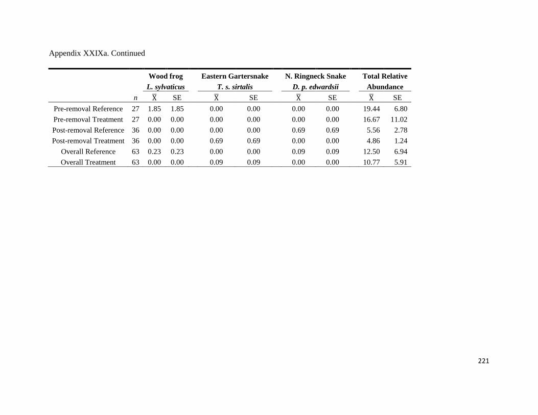
221

Appendix XXIXa. Continued

Wood frog Eastern Gartersnake N. Ringneck Snake Total Relative

L. sylvaticus

T. s. sirtalis

D. p. edwardsii

Abundance

n SE SE SE SE


0.00 0.00

0.00 0.00

19.44 6.80


0.00 0.00

0.00 0.00

16.67 11.02


0.00 0.00

0.69 0.69

5.56 2.78


0.69 0.69

0.00 0.00

4.86 1.24


0.00 0.00

0.09 0.09

12.50 6.94


222

Appendix XXXa: Mean ( ) and SE of herpetofauna relative abundance (No. of captures/100 trap nights) at reference and treatment

cover board arrays at Fort Necessity National Battlefield, Pennsylvania, USA. We trapped using the cover board arrays from 2004

through 2010 during the summer season from May-August. *Post-removal surveys took place following the implementation of

management procedures designed to remove Morrow‟s honeysuckle.

Four-toed Salamander

Northern Slimy Salamander

Red eft

Redback salamander

H. scutatum

P. glutinosus

N. v. viridescens

P. cinereus

n SE SE SE SE


0.00 0.00

3.70 2.45

27.78 7.35


0.00 0.00

0.00 0.00

35.19 6.48


1.39 1.39

4.17 2.18

8.33 2.51


0.00 0.00

2.78 1.87

2.78 1.87


0.70 0.70

3.94 1.36

18.06 5.87


Eastern Gartersnake Eastern Ratsnake

Northern Black Racer

Northern Ringneck Snake

T. s. sirtalis

S. alleghaniensis

C. c. constrictor

D. p. edwardsii

n SE SE SE SE


0.00 0.00

0.00 0.00

0.00 0.00


1.85 1.85

0.00 0.00

0.00 0.00


1.39 1.39

1.39 1.39

2.78 2.78


0.00 0.00

0.00 0.00

0.00 0.00


0.69 0.69

0.69 0.69

1.39 1.39


223

Appendix XXXa. Continued

Smooth Greensnake Total Relative

O. vernalis

Abundance

n SE SE


33.33 6.21


38.89 6.80


27.78 9.48


20.83 11.26


30.56 2.78

Overall Treatment 63 6.25 5.46 29.86 9.03

224

Appendix Ib. Fruit species located during three study arounds at Fort Necessity National

Battlefield, Pennsylvania, USA, from October 2009 – August 2010. Study species were chosen

using a random number generator. When species could not be located in sufficient quantities,

another species was chosen at random to replace it.

Round 1

Round 2

Oct. 20 – Nov. 14, 2009 July 12 – Aug. 6, 2010

Common greenbrier

Staghorn sumac

Smilax rotundifolia

Rhus typhina

Winter grape

Northern dewberry

Vitis cinerea

Rubus flagellaris

Southern arrowwood

Common Serviceberry*

Viburnum dentatum

Amelanchier arborea

Black cherry

Prunus serotina

Flowering dogwood

Cornus florida

Waxy-fruit Hawthorne*

Crataegus pruinosa

Staghorn sumac

Rhus typhina

Poison Ivy*

Toxicodendron radicans

Black gum*

Nyssa sylvatica

*Species present without quantities sufficient for the study

225

Appendix Ic. Values for the environmental variables measured at each foraging station at Fort

Necessity National Battlefield, Pennsylvania, USA, in October – November 2009 (fall) and July

– August 2010 (summer). All values were averaged over 20 stations within each cover type (total

N=60). Averaged values (Mean), standard errors (SE), minimum values (Min) and maximum

values (Max) are reported.

Edge 100 m2 - Summer

Edge 400 m2 - Summer

Variable S.E. Min Max S.E. Min Max

Brush cover (%)

4.25 0.63 1.20 15.00

3.97 0.81 0.00 18.75

Canopy cover (%)

79.93 3.22 46.25 97.50

79.11 3.29 46.25 98.35

Fern cover (%)

7.84 2.76 0.00 45.00

9.15 2.73 0.00 38.75

First sight (cm)

5.99 0.48 5.00 12.50

6.90 1.03 3.00 21.25

Forb cover (%)

17.41 4.00 2.00 63.75

15.70 3.28 5.00 52.50

Grass cover (%)

19.32 3.53 10.00 68.75

18.73 3.27 10.00 62.50

Green cover (%)

47.04 6.42 6.25 97.50

43.38 5.71 8.00 91.25

Leaf cover (%)

28.93 4.15 3.51 67.50

29.11 4.11 4.00 67.50

Log cover (%)

2.27 0.37 1.00 6.25

1.88 0.28 1.00 0.40

Moss cover (%)

3.25 0.33 0.00 7.75

3.10 0.39 0.00 9.50

Road cover (%)

2.38 0.89 1.00 15.00

9.52 1.69 1.00 25.00

Rock cover (%)

1.36 0.18 0.75 5.00

1.40 0.19 0.75 4.25

Shrub cover (%)

9.29 2.48 0.11 46.25

8.01 1.88 5.00 33.75

Shrub distance (m)

4.14 1.61 0.35 25.00

4.14 1.61 0.35 25.00

Shrub stem number

2.05 0.49 1.00 10.00

2.05 0.49 1.00 10.00

Shrub volume (m3)

0.43 0.16 0.02 2.89

0.43 0.16 0.01 2.89

Slope (°)

8.99 1.07 3.25 19.25

8.99 1.07 3.25 19.25

Soil moisture

1.31 0.24 0.13 3.50

1.31 0.24 0.13 3.50

Tallest sight (cm)

22.12 3.00 5.00 47.50

25.69 3.83 5.00 57.50

Tree cover (%)

3.48 0.20 1.51 5.05

3.37 0.26 1.50 6.25

Tree crown (m)

7.96 0.64 2.30 13.20

7.96 0.64 2.30 13.20

Tree DBH (cm)

41.96 6.13 11.15 133.76

41.96 6.13 11.15 133.76

Tree distance (m)

0.94 0.21 0.05 3.30

0.94 0.21 0.05 3.30

Tree height (m)

11.59 0.51 7.00 14.75

11.59 0.51 7.00 14.75

Visitation rate (%)

72.50 6.27 14.29 100.00

72.50 6.27 14.29 100.00

Water (%) 0.00 0.00 0.00 0.00 0.00 0.00 0.00 0.00

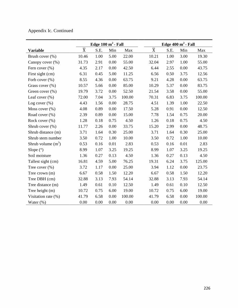
226

Appendix Ic. Continued

Edge 100 m2 - Fall

Edge 400 m2 - Fall


Brush cover (%)

10.46 1.00 5.00 22.00

10.21 1.00 3.00 19.30

Canopy cover (%)

31.73 2.91 0.00 55.00

32.04 2.97 1.00 55.00

Fern cover (%)

4.35 2.17 0.00 42.50

6.44 2.55 0.00 43.75

First sight (cm)

6.31 0.45 5.00 11.25

6.56 0.50 3.75 12.56

Forb cover (%)

8.55 4.36 0.00 63.75

9.21 4.28 0.00 63.75

Grass cover (%)

10.57 5.66 0.00 85.00

10.29 5.37 0.00 83.75

Green cover (%)

19.79 3.72 0.00 52.50

21.54 3.58 0.00 55.00

Leaf cover (%)

72.00 7.04 3.75 100.00

70.31 6.83 3.75 100.00

Log cover (%)

4.43 1.56 0.00 28.75

4.51 1.39 1.00 22.50

Moss cover (%)

4.08 0.89 0.00 17.50

5.28 0.91 0.00 12.50

Road cover (%)

2.39 0.89 0.00 15.00

7.78 1.54 0.75 20.00

Rock cover (%)

1.28 0.18 0.75 4.50

1.26 0.18 0.75 4.50

Shrub cover (%)

11.77 2.26 0.00 33.75

15.20 2.99 0.00 48.75

Shrub distance (m)

3.71 1.64 0.30 25.00

3.71 1.64 0.30 25.00

Shrub stem number

3.50 0.72 1.00 10.00

3.50 0.72 1.00 10.00

Shrub volume (m3)

0.53 0.16 0.01 2.83

0.53 0.16 0.01 2.83

Slope (°)

8.99 1.07 3.25 19.25

8.99 1.07 3.25 19.25

Soil moisture

1.36 0.27 0.13 4.50

1.36 0.27 0.13 4.50

Tallest sight (cm)

16.81 4.59 5.00 76.25

19.31 6.24 3.75 125.00

Tree cover (%)

3.72 1.17 0.00 25.00

3.94 1.12 0.00 23.75

Tree crown (m)

6.67 0.58 1.50 12.20

6.67 0.58 1.50 12.20

Tree DBH (cm)

32.88 3.13 7.93 54.14

32.88 3.13 7.93 54.14

Tree distance (m)

1.49 0.61 0.10 12.50

1.49 0.61 0.10 12.50

Tree height (m)

10.72 0.75 6.00 19.00

10.72 0.75 6.00 19.00

Visitation rate (%)

41.79 6.58 0.00 100.00

41.79 6.58 0.00 100.00

Water (%) 0.00 0.00 0.00 0.00 0.00 0.00 0.00 0.00

227


Field 100 m2 - Summer

Field 400 m2 - Summer


Brush cover (%)

1.20 0.34 0.00 5.00

2.40 0.63 0.00 10.00

Canopy cover (%)

0.25 0.25 0.00 5.00

1.06 0.68 0.00 12.50

Fern cover (%)

0.00 0.00 0.00 0.00

0.00 0.00 0.00 0.00

First sight (cm)

23.88 5.14 6.25 50.00

31.19 7.13 6.25 73.75

Forb cover (%)

70.81 6.35 11.25 100.00

69.77 6.26 11.25 100.00

Grass cover (%)

61.08 7.52 30.00 100.00

60.50 7.37 31.75 100.00

Green cover (%)

94.19 0.91 85.00 100.00

93.25 1.33 75.00 100.00

Leaf cover (%)

3.88 1.35 0.00 27.50

3.56 1.26 0.00 25.00

Log cover (%)

0.04 0.04 0.00 0.75

0.00 0.00 0.00 0.00

Moss cover (%)

0.40 0.28 0.00 5.00

0.40 0.28 0.00 5.00

Road cover (%)

0.00 0.00 0.00 0.00

0.00 0.00 0.00 0.00

Rock cover (%)

3.00 0.62 0.00 10.00

3.24 0.60 0.00 9.50

Shrub cover (%)

17.34 6.09 0.00 90.00

20.30 5.61 0.00 78.75

Shrub distance (m)

3.97 0.84 0.20 13.40

3.97 0.84 0.20 13.40

Shrub stem number

8.05 1.10 2.00 20.00

8.05 1.10 2.00 20.00

Shrub volume (m3)

3.27 1.22 0.16 25.07

3.27 1.22 0.16 25.07

Slope (°)

2.56 0.58 0.25 8.85

2.56 0.57 0.25 8.85

Soil moisture

1.90 0.21 0.25 3.88

1.90 0.21 0.25 3.88

Tallest sight (cm)

76.25 2.90 18.75 121.25

95.31 4.43 40.00 145.00

Tree cover (%)

0.15 0.08 0.00 1.25

0.54 0.21 0.00 2.75

Tree crown (m)

7.16 0.73 2.50 14.00

7.16 0.73 2.50 14.00

Tree DBH (cm)

23.57 2.95 4.78 57.32

23.57 2.95 4.78 57.32

Tree distance (m)

15.19 2.79 0.40 45.00

15.19 2.79 0.40 45.00

Tree height (m)

8.07 0.73 2.50 13.60

8.07 0.73 2.50 13.60

Visitation rate (%)

37.60 6.06 0.00 92.86

37.60 6.06 0.00 92.86

Water (%) 0.00 0.00 0.00 0.00 0.00 0.00 0.00 0.00

228


Field 100 m2 - Fall

Field 400 m

2 - Fall


Brush cover (%)

55.19 5.16 0.00 92.50

56.88 5.26 0.00 88.75

Canopy cover (%)

1.00 1.00 0.00 20.00

2.35 1.62 0.00 25.00

Fern cover (%)

0.11 0.08 0.00 1.50

0.20 0.16 0.00 3.25

First sight (cm)

7.69 5.74 5.00 15.00

10.74 9.11 5.00 41.25

Forb cover (%)

46.02 5.61 3.00 80.00

44.85 5.26 3.75 80.00

Grass cover (%)

47.63 5.71 5.00 95.00

47.54 5.58 7.00 90.00

Green cover (%)

28.61 3.22 0.00 47.50

27.51 3.22 0.00 51.25

Leaf cover (%)

3.96 1.44 0.00 17.25

5.00 1.32 0.00 15.00

Log cover (%)

0.00 0.00 0.00 0.00

0.09 0.09 0.00 1.75

Moss cover (%)

0.54 0.26 0.00 4.00

0.88 0.34 0.00 4.50

Road cover (%)

0.00 0.00 0.00 0.00

0.00 0.00 0.00 0.00

Rock cover (%)

5.39 0.87 0.00 11.00

5.95 0.87 0.00 11.50

Shrub cover (%)

21.76 6.78 0.00 95.00

28.98 7.00 5.00 90.00

Shrub distance (m)

3.05 0.57 0.20 11.00

3.05 0.57 0.20 11.00

Shrub stem number

10.45 2.15 1.00 43.00

10.45 2.15 1.00 43.00

Shrub volume (m3)

5.99 2.22 0.02 35.78

5.99 2.22 0.02 35.78

Slope (°)

2.53 0.58 0.00 8.75

2.53 0.58 0.00 8.75

Soil moisture

1.90 0.21 0.25 3.88

1.90 0.21 0.25 3.88

Tallest sight (cm)

42.81 0.68 7.50 93.75

70.00 1.92 15.00 155.00

Tree cover (%)

0.23 0.16 0.00 3.00

0.65 0.30 0.00 5.50

Tree crown (m)

7.43 0.70 2.50 14.00

7.43 0.70 2.50 14.00

Tree DBH (cm)

32.22 4.15 4.78 73.25

32.22 4.15 4.78 73.25

Tree distance (m)

15.19 2.83 0.40 45.00

15.19 2.83 0.40 45.00

Tree height (m)

10.14 0.95 5.00 21.00

10.14 0.95 5.00 21.00

Visitation rate (%)

61.43 5.94 14.29 100.00

61.43 5.94 14.29 100.00

Water (%) 0.00 0.00 0.00 0.00 0.00 0.00 0.00 0.00

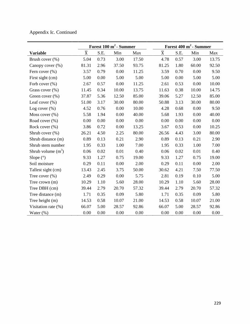
229


Forest 100 m2 - Summer

Forest 400 m

2 - Summer


Brush cover (%)

5.04 0.73 3.00 17.50

4.78 0.57 3.00 13.75

Canopy cover (%)

81.31 2.96 37.50 93.75

81.25 1.80 60.00 92.50

Fern cover (%)

3.57 0.79 0.00 11.25

3.59 0.70 0.00 9.50

First sight (cm)

5.00 0.00 5.00 5.00

5.00 0.00 5.00 5.00

Forb cover (%)

2.67 0.57 0.00 11.25

2.61 0.53 0.00 10.00

Grass cover (%)

11.45 0.34 10.00 13.75

11.63 0.38 10.00 14.75

Green cover (%)

37.87 5.36 12.50 85.00

39.06 5.27 12.50 85.00

Leaf cover (%)

51.00 3.17 30.00 80.00

50.88 3.13 30.00 80.00

Log cover (%)

4.52 0.76 0.00 10.00

4.28 0.68 0.00 9.50

Moss cover (%)

5.58 1.94 0.00 40.00

5.68 1.93 0.00 40.00

Road cover (%)

0.00 0.00 0.00 0.00

0.00 0.00 0.00 0.00

Rock cover (%)

3.86 0.72 0.00 13.25

3.67 0.53 0.00 10.25

Shrub cover (%)

26.21 4.50 2.25 80.00

26.56 4.43 3.00 80.00

Shrub distance (m)

0.89 0.13 0.21 2.90

0.89 0.13 0.21 2.90

Shrub stem number

1.95 0.33 1.00 7.00

1.95 0.33 1.00 7.00

Shrub volume (m3)

0.06 0.02 0.01 0.40

0.06 0.02 0.01 0.40

Slope (°)

9.33 1.27 0.75 19.00

9.33 1.27 0.75 19.00

Soil moisture

0.29 0.11 0.00 2.00

0.29 0.11 0.00 2.00

Tallest sight (cm)

13.43 2.45 3.75 50.00

30.62 4.21 7.50 77.50

Tree cover (%)

2.49 0.29 0.00 5.75

2.81 0.19 0.10 5.00

Tree crown (m)

10.29 1.10 5.60 28.00

10.29 1.10 5.60 28.00

Tree DBH (cm)

39.44 2.79 20.70 57.32

39.44 2.79 20.70 57.32

Tree distance (m)

1.71 0.35 0.09 5.80

1.71 0.35 0.09 5.80

Tree height (m)

14.53 0.58 10.07 21.00

14.53 0.58 10.07 21.00

Visitation rate (%)

66.07 5.00 28.57 92.86

66.07 5.00 28.57 92.86

Water (%) 0.00 0.00 0.00 0.00 0.00 0.00 0.00 0.00

230


Forest 100 m

2 - Fall

Forest 400 m

2 - Fall


Brush cover (%)

53.71 8.56 3.50 95.00

53.90 8.58 3.50 95.00

Canopy cover (%)

31.87 4.53 6.25 85.00

29.43 2.83 16.25 63.75

Fern cover (%)

1.79 0.46 0.00 6.50

2.10 0.49 7.00 0.00

First sight (cm)

6.25 0.36 5.00 10.00

6.25 0.36 5.00 10.00

Forb cover (%)

0.67 0.24 0.00 3.00

0.67 0.24 3.00 0.00

Grass cover (%)

1.05 0.31 0.00 4.00

1.04 0.30 0.00 3.25

Green cover (%)

21.41 4.70 3.00 87.50

22.61 5.02 3.00 90.00

Leaf cover (%)

84.86 3.09 36.25 100.00

84.36 3.13 36.25 95.00

Log cover (%)

4.62 0.71 0.00 11.25

4.89 0.78 0.00 11.25

Moss cover (%)

9.14 4.45 1.50 87.50

9.73 4.59 1.50 90.00

Road cover (%)

0.00 0.00 0.00 0.00

0.00 0.00 0.00 0.00

Rock cover (%)

1.98 0.25 0.00 5.00

1.99 0.24 1.00 5.00

Shrub cover (%)

16.54 3.56 0.00 65.00

16.62 3.63 0.00 58.75

Shrub distance (m)

2.48 1.23 0.10 25.00

2.48 1.23 0.10 25.00

Shrub stem number

2.00 0.42 1.00 9.00

2.00 0.42 1.00 9.00

Shrub volume (m3)

0.56 0.32 0.01 6.08

0.56 0.32 0.01 6.08

Slope (°)

9.33 1.27 0.75 19.00

9.33 1.27 0.75 19.00

Soil moisture

23.25 0.06 0.00 1.13

23.25 0.06 0.00 1.13

Tallest sight (cm)

17.43 3.39 5.00 55.00

20.00 2.87 5.00 43.75

Tree cover (%)

4.66 0.16 3.50 5.75

4.61 0.15 3.50 5.75

Tree crown (m)

13.38 2.20 3.20 36.30

13.38 2.20 3.20 36.30

Tree DBH (cm)

57.10 9.76 14.01 187.90

57.10 9.76 14.01 187.90

Tree distance (m)

2.61 0.58 0.30 9.10

2.61 0.58 0.30 9.10

Tree height (m)

18.75 1.15 7.00 28.00

18.75 1.15 7.00 28.00

Visitation rate (%)

59.65 5.91 0.00 85.71

59.65 5.91 0.00 85.71

Water (%) 0.00 0.00 0.00 0.00 0.00 0.00 0.00 0.00

evaluating the effects of morrow's honeysuckle control on

Documents