evaluation of a deterministic boltzmann solver for radiation therapy

Evaluation of a deterministic Boltzmann solver for radiation therapy dose

calculations involving high-density hip prostheses

by

Samantha AM Lloyd

BSc, Thompson Rivers University, 2009

A Thesis Submitted in Partial Fulfillment of the

Requirements for the Degree of

MASTER OF SCIENCE

in the Department of Physics and Astronomy

c© Samantha AM Lloyd, 2011

University of Victoria

All rights reserved. This thesis may not be reproduced in whole or in part, by

photocopying or other means, without the permission of the author.

ii

Evaluation of a deterministic Boltzmann solver for radiation therapy dose

calculations involving high-density hip prostheses

by

Samantha AM Lloyd

BSc, Thompson Rivers University, 2009

Supervisory Committee

Dr. W. Ansbacher, Co-supervisor

(Department of Physics and Astronomy)

(British Columbia Cancer Agency - Vancouver Island Centre)

Dr. A. Jirasek, Co-supervisor


Dr. P. Basran, Member



iii

Supervisory Committee

Dr. W. Ansbacher, Co-supervisor



Dr. A. Jirasek, Co-supervisor


Dr. P. Basran, Member



ABSTRACT

Acuros R© External Beam (Acuros XB) is a new radiation dose calculation algo-

rithm available as part of Varian Medical Systems’ radiotherapy treatment planning

system, ECLIPSETM. Acuros XB calculates dose distributions by finding the de-

terministic solution to the linear Boltzmann transport equation which governs the

transport of particles or radiation through matter. Among other things, Acuros XB

claims an ability to accurately model dose perturbations due to increased photon and

electron scatter within a high-density volume, such as a hip prosthesis. Until now, the

only way to accurately model high-density scatter was with a Monte Carlo simulation

which gives the stochastic solution to the same transport equation, but is time and

computationally expensive. In contrast, Acuros XB solves the transport equation at

time scales appropriate for clinical use.

An evaluation of Acuros XB for radiation dose calculations involving high-density

objects was undertaken using EGSnrc based Monte Carlo as the benchmark. Calcula-

tions were performed for geometrically ideal virtual phantoms, water tank phantoms

containing cylindrical steel rods and hip prostheses, and for a clinical prostate treat-

ment plan involving a unilateral prosthetic hip. The anisotropic analytical algorithm

iv

(AAA), a convolution-superposition algorithm used for treatment planning at the

British Columbia Cancer Agency’s Vancouver Island Center, was also used to illus-

trate the limitations of current radiotherapy planning tools. In addition, to verify

the qualitative properties of dose perturbations due to high-density volumes, film

measurements were taken and compared to Monte Carlo, Acuros XB and AAA data.

Dose distributions calculated with Acuros XB agree very well with distributions

calculated with Monte Carlo. γ-analyses performed at 2% and 2 mm using Monte

Carlo as the reference dose were within tolerance for 92–99% of voxels considered.

AAA, on the other hand, was within tolerance for 61–97% of voxels considered under

the same γ-constraints. For the clinical prostate plan, AAA produced localized dose

underestimates that were absent when calculated by Acuros XB. As well, both Monte

Carlo and Acuros XB showed very good agreement with the film measurements,

while AAA showed large discrepancies at and beyond the location of measured dose

perturbations.

Acuros XB has been shown to handle does perturbations due to high-density

volumes as well as Monte Carlo, at clinically appropriate time scales, and better than

the current algorithm used for treatment planning at the Vancouver Island Center.

v

Contents

Supervisory Committee ii

Abstract iii

Table of Contents v

List of Tables vii

List of Figures viii

Acknowledgements xi

1 Introduction 1

1.1 Radiation Therapy . . . . . . . . . . . . . . . . . . . . . . . . . . . . 1

1.1.1 Radiation Therapy Treatment Planning . . . . . . . . . . . . . 3

1.1.2 Dose Calculation Algorithms . . . . . . . . . . . . . . . . . . . 5

1.2 High Density Implants . . . . . . . . . . . . . . . . . . . . . . . . . . 6

1.3 Thesis Scope . . . . . . . . . . . . . . . . . . . . . . . . . . . . . . . . 8

2 Theory 10

2.1 Particle Interactions . . . . . . . . . . . . . . . . . . . . . . . . . . . 10

2.1.1 Photon Interactions . . . . . . . . . . . . . . . . . . . . . . . . 10

2.1.2 Electron Interactions . . . . . . . . . . . . . . . . . . . . . . . 13

2.2 Dose Calculation Algorithms . . . . . . . . . . . . . . . . . . . . . . . 15

2.2.1 Convolution-Superposition Algorithms . . . . . . . . . . . . . 15

2.2.2 Linear Boltzmann Transport Equation . . . . . . . . . . . . . 16

2.3 Imaging and Contouring . . . . . . . . . . . . . . . . . . . . . . . . . 19

2.3.1 Computed Tomography & Hounsfield Unit Saturation . . . . . 19

2.3.2 Pixelation . . . . . . . . . . . . . . . . . . . . . . . . . . . . . 20

2.3.3 Contouring . . . . . . . . . . . . . . . . . . . . . . . . . . . . 21

vi

2.4 Radio-chromic Film . . . . . . . . . . . . . . . . . . . . . . . . . . . . 21

2.5 Summary . . . . . . . . . . . . . . . . . . . . . . . . . . . . . . . . . 22

3 Methods & Materials 23

3.1 Modeling Environments & Parameters . . . . . . . . . . . . . . . . . 23

3.1.1 Introduction . . . . . . . . . . . . . . . . . . . . . . . . . . . . 23

3.1.2 Source Model . . . . . . . . . . . . . . . . . . . . . . . . . . . 24

3.1.3 Material Data . . . . . . . . . . . . . . . . . . . . . . . . . . . 25

3.1.4 Interactions & Approximations . . . . . . . . . . . . . . . . . 27

3.2 Experimental Measurements . . . . . . . . . . . . . . . . . . . . . . . 29

3.3 Experimental Calculations . . . . . . . . . . . . . . . . . . . . . . . . 32

3.3.1 Virtual Phantoms . . . . . . . . . . . . . . . . . . . . . . . . . 32

3.3.2 Water Tank Phantoms . . . . . . . . . . . . . . . . . . . . . . 33

3.3.3 Clinical Patient Data Set . . . . . . . . . . . . . . . . . . . . . 36

3.4 Reporting Methods . . . . . . . . . . . . . . . . . . . . . . . . . . . . 37

3.4.1 Profile & Depth Doses . . . . . . . . . . . . . . . . . . . . . . 37

3.4.2 γ Evaluations . . . . . . . . . . . . . . . . . . . . . . . . . . . 37

4 Results 39

4.1 Film Measurements . . . . . . . . . . . . . . . . . . . . . . . . . . . . 39

4.2 Virtual Phantoms . . . . . . . . . . . . . . . . . . . . . . . . . . . . . 40

4.3 Water Phantoms . . . . . . . . . . . . . . . . . . . . . . . . . . . . . 54

4.4 Patient Case . . . . . . . . . . . . . . . . . . . . . . . . . . . . . . . . 60

4.5 Computation time . . . . . . . . . . . . . . . . . . . . . . . . . . . . 63

5 Discussion of Results 64

5.1 Virtual Phantoms . . . . . . . . . . . . . . . . . . . . . . . . . . . . . 65

5.2 Water Phantoms . . . . . . . . . . . . . . . . . . . . . . . . . . . . . 66

5.3 Patient Case . . . . . . . . . . . . . . . . . . . . . . . . . . . . . . . . 67

5.4 Summary . . . . . . . . . . . . . . . . . . . . . . . . . . . . . . . . . 68

6 Conclusions & Considerations 69

A Material Information 72

Bibliography 75

vii

List of Tables

Table 3.1 Material properties for muscle, titanium, stainless steel and Co-

Cr-Mo. . . . . . . . . . . . . . . . . . . . . . . . . . . . . . . . . 26

Table 3.2 Materials and corresponding density ranges for Eclipse and EGSnrc

Monte Carlo. . . . . . . . . . . . . . . . . . . . . . . . . . . . . 27

Table 4.1 γ-analysis results for 20x20x20 cm3 virtual phantoms at 2% and

2 mm as calculated by Acuros XB and AAA referenced against

Monte Carlo. . . . . . . . . . . . . . . . . . . . . . . . . . . . . 51

Table 4.2 Characterization of back-scatter and lateral-scatter peaks due to

stainless steel and titanium alloy inhomogeneities. . . . . . . . . 51

Table 4.3 γ-analyses results for water phantoms at 2% and 2 mm as calcu-

lated by Acuros XB and AAA referenced against Monte Carlo. . 54

Table 4.4 Computation times for Monte Carlo, AAA and Acuros XB . . . 63

Table A.1 Material compositions for EGSnrc and Acuros XB. . . . . . . . 72

viii

List of Figures

Figure 1.1 Varian Clinac 21EX linear accelerator. . . . . . . . . . . . . . . 2

Figure 1.2 Slice of a CT image used for radiotherapy planning. . . . . . . . 4

Figure 1.3 Example of a radiation therapy treatment plan and calculated

dose distribution overlaid on a CT image. . . . . . . . . . . . . 4

Figure 1.4 Photograph and radiograph of typical hip prostheses. . . . . . . 6

Figure 1.5 Example of a dose distribution perturbed by the presence of a

high-density object. . . . . . . . . . . . . . . . . . . . . . . . . 7

Figure 2.1 Schematic of a Compton scattering event. . . . . . . . . . . . . 11

Figure 2.2 Schematic of an electron soft interaction. . . . . . . . . . . . . . 14

Figure 2.3 Spatial interpretation of a 2-D data set. . . . . . . . . . . . . . 20

Figure 3.1 HU to mass- and electron-density conversion curves for Eclipse

and EGSnrc Monte Carlo. . . . . . . . . . . . . . . . . . . . . . 26

Figure 3.2 Depth dose perturbation data included in AAPM TG Report 63.

Reproduced with permission. . . . . . . . . . . . . . . . . . . . 29

Figure 3.3 Illustration of the experimental setup used to measure high-

density forward scatter due to a 10x10 cm2 field of 18 MV pho-

tons steel. . . . . . . . . . . . . . . . . . . . . . . . . . . . . . . 30

Figure 3.4 Calibration curve for Gafchromic R© EBT2 radio-chromic dosi-

metric film. . . . . . . . . . . . . . . . . . . . . . . . . . . . . . 31

Figure 3.5 A 20x20x20 cm3 virtual skeletal muscle phantom containing a

stainless steel rod centre. . . . . . . . . . . . . . . . . . . . . . 32

Figure 3.6 Steel rod and hip prostheses imaged for calculation comparisons. 33

Figure 3.7 Eclipse generated structure set for a plexiglass water tank con-

taining cylindrical stainless steel rods. . . . . . . . . . . . . . . 34

Figure 3.8 Plexiglass water tank containing hip prostheses and correspond-

ing Eclipse generated structure set. . . . . . . . . . . . . . . . . 35

ix

Figure 3.9 Contoured planning CT for an anonymized prostate patient with

a unilateral hip prosthesis. . . . . . . . . . . . . . . . . . . . . . 36

Figure 4.1 Film measurements and Acuros XB, AAA and EGSnrc Monte

Carlo data for the high-density inhomogeneity outlined in Figure

3.2 . . . . . . . . . . . . . . . . . . . . . . . . . . . . . . . . . . 40

Figure 4.2 Depth dose plot for 18 MV photons through a 20x20x20 cm3

skeletal muscle phantom containing stainless steel. . . . . . . . 41

Figure 4.3 Dose profile plot for 18 MV photons through a 20x20x20 cm3


Figure 4.4 Depth dose plot for 6 MV photons through a 20x20x20 cm3 skele-

tal muscle phantom containing stainless steel. . . . . . . . . . . 44



Figure 4.6 Profile and depth dose for 18 MV photons with a 10 gantry rota-

tion through a 20x20x20 cm3 skeletal muscle phantom containing

stainless steel. . . . . . . . . . . . . . . . . . . . . . . . . . . . . 46

Figure 4.7 Depth dose plot for 18 MV photons through a 20x20x20 cm3

skeletal muscle phantom containing titanium alloy. . . . . . . . 47



Figure 4.9 Depth dose plot for 6 MV photons through a 20x20x20 cm3 skele-

tal muscle phantom containing titanium alloy. . . . . . . . . . . 49

Figure 4.10Dose profile plot for 6 MV photons through a 20x20x20 cm3


Figure 4.11Profile and depth dose for 18MV photons through a 10x10x10

cm3 skeletal muscle phantom containing stainless steel. . . . . . 53

Figure 4.12Percent dose difference and γ-factor distribution for 18 MV pho-

tons through a stainless steel rod as calculated by Acuros XB

compared with Monte Carlo. . . . . . . . . . . . . . . . . . . . 55


tons through a stainless steel rod as calculated by AAA compared

with Monte Carlo. . . . . . . . . . . . . . . . . . . . . . . . . . 56

x


tons through a steel alloy hip prosthesis as calculated by Acuros

XB compared with Monte Carlo. . . . . . . . . . . . . . . . . . 57


tons through a titanium alloy hip prosthesis as calculated by

Acuros XB compared with Monte Carlo. . . . . . . . . . . . . . 58

Figure 4.16γ-factor distributions for 18 MV photons through steel and tita-

nium alloy hip prostheses as calculated by AAA compared with

Monte Carlo. . . . . . . . . . . . . . . . . . . . . . . . . . . . . 59

Figure 4.17Treatment plan field arrangement for prostate patient with uni-

lateral hip prosthesis. . . . . . . . . . . . . . . . . . . . . . . . 60

Figure 4.18Percent dose difference and γ-factor distribution for a prostate

treatment plan as calculated by AAA and Monte Carlo. . . . . 61

Figure 4.19Percent dose difference and γ-factor distribution for a prostate

treatment plan as calculated by Acuros XB and Monte Carlo. . 62

xi

Acknowledgments

My sincerest thanks go to my supervisory committee for all their feedback and

support. This work would have been impossible without the guidance and infinite

patience of Will Ansbacher and Karl Bush. Thanks to Sergei Zavgorodni for the

Monte Carlo help and the hard questions, and to everyone else at the BC Cancer

Agency’s Vancouver Island Centre - physicists, students and support staff - for setting

examples of passion, dedication and excellence. You’ve all given me a lot to live up

to.

Additional thanks to Dr. Reft and the AAPM for allowing me to use a figure from

their Task Group Report, and to Varian Medical Systems for providing Eclipse and

Acuros XB. This work has been supported, in part, by an Alexander Graham Bell

Canada Graduate Scholarship from the Natural Sciences and Engineering Research

Council of Canada.

Chapter 1

Introduction

Approximately half of the 45% of Canadian men and 40% of Canadian women who

develop cancer during their lifetime will receive radiation therapy as part of their

treatment [1, 2]. Medical physicists and radiotherapy treatment planners use sophis-

ticated dose calculation algorithms to simulate the distribution of radiation dose for

a treatment plan to ensure treatment efficacy and patient safety. Acuros R© External

Beam (Acuros XB) is a novel dose calculation algorithm available from the commer-

cial vendor, Varian Medical Systems [3]. Among other things, Acuros XB should

be an improvement over current clinical algorithms for calculations involving high-

density implants. Until now, there has been no reliable, clinically appropriate method

of accurately modeling the dose perturbations that arise due to increased photon and

electron scatter in high-density materials.

The aim of this work is to evaluate the accuracy of Acuros XB for dose calculations

involving high-density objects, specifically hip prostheses, by comparison with Monte

Carlo. The following chapter provides a brief overview of radiation therapy physics,

hip prostheses and their impact on radiotherapy planning, and a summary of the

thesis scope.

1.1 Radiation Therapy

Radiation therapy, or radiotherapy, is the targeted delivery of highly energetic photons

or particles to a specific patient volume with the purpose of destroying cancerous cells

within healthy tissue. It can be an internal or an external treatment, making use of

radioactive isotopes that emit energetic photons or particles as they decay, or by

2

producing and delivering energetic photons or particles with a medical accelerator.

Used alone, radiation therapy is capable of curing many cancers and can be safely

used in concert with other therapies such as surgery and pharmaceuticals. In addition,

palliative radiotherapy can greatly reduce the pain associated with tumour growth in

late stages of the disease, significantly improving quality-of-life for patients receiving

end-of-life care.

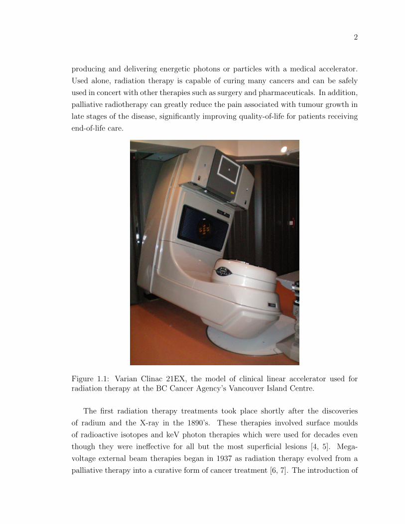
Figure 1.1: Varian Clinac 21EX, the model of clinical linear accelerator used forradiation therapy at the BC Cancer Agency’s Vancouver Island Centre.

The first radiation therapy treatments took place shortly after the discoveries

of radium and the X-ray in the 1890’s. These therapies involved surface moulds

of radioactive isotopes and keV photon therapies which were used for decades even

though they were ineffective for all but the most superficial lesions [4, 5]. Mega-

voltage external beam therapies began in 1937 as radiation therapy evolved from a

palliative therapy into a curative form of cancer treatment [6, 7]. The introduction of

3

the first cobalt-60 therapy units in Saskatchewan and Ontario in 1951 followed by the

first clinical linear accelerator used in London in 1953 set the stage for the external

beam mega-voltage therapies that are not only still in use, but are the dominant

technique for therapeutic radiation delivery [6, 8, 9]. Consequently, external-beam,

mega-voltage radiation therapy is the focus of this work. An example of a medical

linear accelerator used at the BC Cancer Agency’s Vancouver Island Centre (VIC) is

shown in Figure 1.1.

Today, spectral 6 MV and 18 MV photon beams are delivered with millimetre

precision at escalating prescribed doses and in more complex geometries than ever

before. The precision and quality of these treatments are limited by the daily repro-

ducibility of patient position in the radiation field, the ability to locate and delineate

the tumour volume on a planning image and the accuracy with which planners can

predict the resulting dose distribution within a patient. Accurate treatment planning

is a critical precursor to ensuring maximum tumour coverage while mitigating the

severity of side effects and probability of secondary cancers caused by normal tissue

exposure. What follows are descriptions of the treatment planning process and the

algorithms used to simulate radiotherapy delivery.

1.1.1 Radiation Therapy Treatment Planning

Radiotherapy planning is done, for the most part, using sophisticated image rendering

and dose calculation software packages called treatment planning systems. The pro-

cess begins with a medical image, usually an x-ray computed tomography (CT) image

such as that in Figure 1.2, on which a team of radiation oncologists and radiotherapy

planners, or dosimetrists, delineate the volumes to be treated and critical organs to

be spared. Based on these contours, the dosimetrist uses the planning system to set

the positions and properties of external photon beams and employs a dose calcula-

tion algorithm to model the resulting dose distribution. An example of a treatment

plan and dose distribution is shown in Figure 1.3. The planning team may evaluate

the quality of the plan based on the simulated dose distribution and make necessary

modifications until a satisfactory distribution is produced. Acceptance criteria for

a treatment plan depend on the delivery technique used but often include a homo-

geneous target dose as well as upper dose limits for proportional volumes of at-risk

organs, for example, no more than 20% of a particular organ may receive more than

30 Gy. Once an acceptable treatment plan has been approved by the radiation on-

4

Figure 1.2: Slice of a CT image used for radiotherapy planning.

cologist and, if necessary, a medical physicist, it is transfered to the linear accelerator

control console for delivery.

The radiation therapy plan that a patient ultimately receives is dependent on the

modeling algorithm’s representation of the resulting dose distribution. Consequently,

the quality and efficacy of a radiotherapy plan hinges on the ability of a dose calcu-

lation algorithm to accurately model dose deposition. Naturally, medical physicists

are constantly improving existing algorithms and employing new techniques to bridge

the gap between radiotherapy models and reality.

Figure 1.3: Example of a radiation therapy treatment plan and calculated dose dis-tribution overlaid on a CT image.

5

1.1.2 Dose Calculation Algorithms

Modern dose calculation algorithms generally fall into two categories: convolution-

superposition or Boltzmann-solvers. Both types of algorithm base their calculations

on the material properties contained in the planning image and the physical interac-

tions that govern the transport of radiation through media, though some algorithms

are better at modeling these interactions than others. The dominant particle interac-

tions in radiotherapy include the photoelectric effect, where a photon interacts with

an electron, imparting all of its energy to the secondary electron; Compton scattering,

where a photon interacts with an electron imparting some energy to the secondary

electron while retaining part of its initial energy; pair production, where a photon in-

teracts with an atomic nucleus to produce and electron-positron pair; bremsstrahlung

radiation, where an electron interacts with an atomic nucleus to produce a photon;

and electron scattering. These interactions are discussed in greater detail in Chapter

2. [8, 10]

Convolution-superposition algorithms model the attenuation of primary photons

through a volume of interest before using one or more measurement or Monte Carlo

generated scatter kernels to determine the resulting dose deposition [5]. Because

much of the calculation or measurement is done beforehand, convolution algorithms

are characteristically fast and well-suited to clinical environments. The solutions

they provide are based on acceptable approximations for most patient volumes and

treatment techniques.

Boltzmann-solvers are algorithms that directly solve the Linear Boltzmann Trans-

port Equation (LBTE), a set of partial differential equations that govern the transport

of particles or radiation through matter. Monte Carlo is the best known Boltzmann-

solver, providing a stochastic solution to LBTE. A random number generator is used

to sample the properties and interactions of particles as they are transported explicitly

through a volume of interest. Monte Carlo simulations are generally accepted as the

most accurate model of particle transport and dose deposition, however, because the

history of each primary and secondary particle is modeled explicitly, calculations are

characteristically slow and usually reserved for research applications. Acuros XB is

the newest commercial, medical purpose Boltzmann-solver, providing a deterministic

solution to the LBTE. Chapter 2 provides a detailed discussion of the Boltzmann-

solvers and of convolution-superposition algorithms. [3]

6

1.2 High Density Implants

Dental fillings, metal plates, portacaths and pacemakers are just a few examples of

high-density implants that may be found in the human body. The presence of a high-

density object in a radiation field causes significant perturbations to the resulting

dose distribution, so high-density implants are a matter of concern in radiotherapy

treatment planning. Due to their size and inevitable involvement in pelvic irradiation,

hip prostheses are of particular interest to planners and physicists.

Figure 1.4: Photograph (top) and radiograph (bottom) of typical hip prostheses.

Hip prostheses have three parts: a femoral stem, head and acetabular cup. Some

patients have only the stem while others have all three parts. The head is typically

made of a polyethylene core with a metal shell of titanium alloy, steel or Co-Cr-

Mo. The stem and head are typically made of titanium alloy, steel or Co-Cr-Mo

and may be solid or hollow. [11] A typical hip prosthesis and radiograph of an

implanted prothesis are displayed in Figure 1.4. CT images of high-density objects

are notoriously corrupted by streaking and shadowing artifacts that result from the

7

complete attenuation of imaging x-rays by the high-density material, as demonstrated

in Figure 1.2.

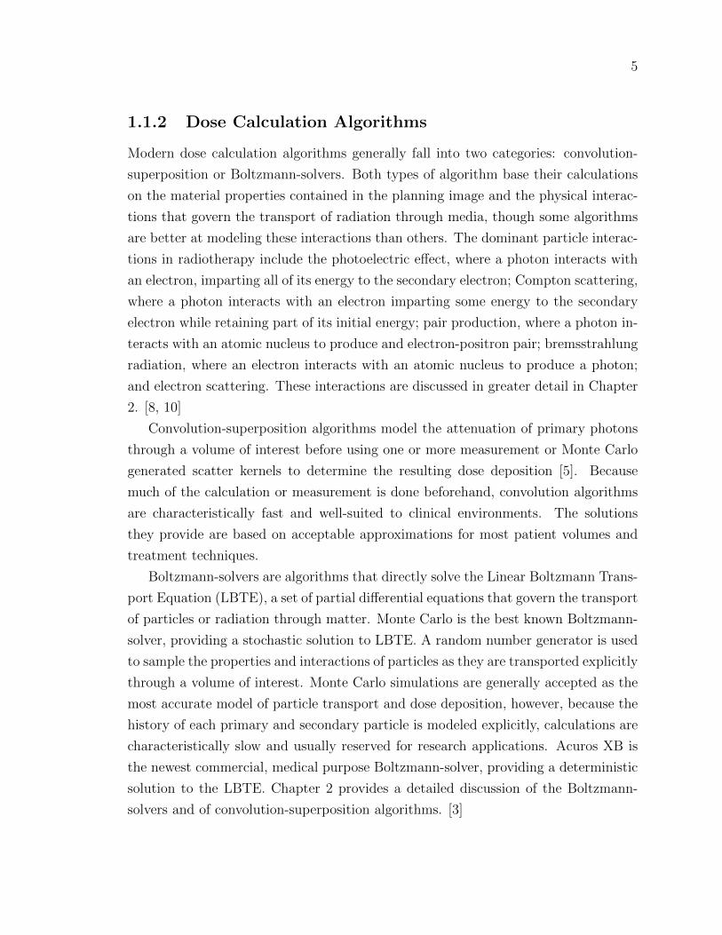
Figure 1.5: Example of a depth dose (top) and dose profile (bottom) perturbed bythe presence of a high-density object. Both data sets were generated using EGSnrcbased Monte Carlo.

Figure 1.5 displays the depth dose (top) and dose profile (bottom) plots for a

square 18 MV field through a phantom generated by Monte Carlo simulations. The

8

black curves are data for a homogeneous phantom while the green curves show the

perturbations that result from a square high-density inhomogeneity, contained within

the vertical black lines. The presence of the inhomogeneity causes an increase in

photon attenuation, increasing the number of secondary photons and electrons which,

in turn, interact more frequently within the high-density object. This has a number of

effects: the equilibrium of forward-backward and right-left scattered electrons breaks

down at the material interfaces producing dose build-down and build-up effects, the

increased number and scattering of electrons in the implant means an increase in the

number of electrons leaving the high-density object causing dramatic dose peaks on

the top and lateral surfaces of the inhomogeneity, and the increased attenuation of

primary photons results in lower dose beyond the high-density region.

Monte Carlo systems are known to model high-density scatter very accurately

[11]. Unfortunately, Monte Carlo calculations are too computationally expensive

for clinical use. The convolution-superposition algorithms used in clinics for daily

treatment planning are capable of correcting for some inhomogeneities, but these

corrections are insufficient when dealing with very high-density materials such as

titanium alloy or steel and grossly underestimate the resulting dose perturbations.

Pelvic patients who have had one or both hips replaced with prostheses often receive

an optimal treatment technique that has been coarsely adapted to avoid treating

through the prosthesis and corrected, approximately, to account for dose shadowing

and increased interface doses.

1.3 Thesis Scope

In November 2010, Varian Medical Systems received clearance from the US Food and

Drug Administration to market their new dose calculation algorithm, Acuros XB.

Based on the general purpose radiation transport modeling system, Attila R©, first

developed at Los Alamos National Laboratory in Los Alamos, New Mexico, Acuros

XB has been modified and optimized for radiation therapy planning calculations

[3, 12].

Four teams of physicists world-wide, including a team at VIC, were selected to

perform the pre-release verification of Acuros XB version 11.0 as implemented in

ECLIPSETM, Varian’s treatment planning system. These evaluations have been un-

derway for just over a year and are producing extremely encouraging results [13, 14].

As part of this investigation, and as the objective of this thesis, the ability of Acuros

9

XB to accurately model dose perturbations due to the presence of a high-density ob-

ject is evaluated. This evaluation is done, principally, against EGSnrc-based Monte

Carlo using single, open fields incident on tissue volumes containing high-density

geometries of varying complexity. In addition, a set of radio-chromic film measure-

ments are included to qualitatively verify the shape of the high-density perturbation

with depth. To illustrate the impact of high-density perturbations on clinical work,

an anonymized prostate treatment plan is re-calculated with Acuros XB and Monte

Carlo and evaluated.

The current dose calculation algorithm used for treatment planning at VIC is the

anisotropic analytical algorithm (AAA), one of the leading convolution-superposition

calculation techniques available. AAA has been extensively evaluated and has per-

formed very well for most clinical cases [15, 16]. The inclusion of AAA data in this

work is to highlight current algorithm limitations and the advantages of a clinical

algorithm designed to handle high-density perturbations.

Chapter 2 will discuss, in detail, the photon and particle interactions that take

place during radiation therapy and the ways in which the dose calculation algorithms

attempt to model them. As well, image acquisition and modification for treatment

planning and radio-chromic film dosimetry will be covered.

Chapter 3 outlines the implementations of Acuros XB, Monte Carlo and AAA and

their associated user-defined settings. As well, Chapter 3 includes descriptions of all

the experimental set ups, from film measurement calibrations to prostate contours,

concluding with an explanation of the γ-analysis which will be used in Chapter 4.

Chapter 4 presents all of the measured and calculated experimental data, as well as

analyses, while Chapter 5 is a discussion of the results and their significance. Chapter

6 will conclude with an overall assessment of Acuros XB and its performance, as well

as remaining concerns and considerations.

10

Chapter 2

Theory

This chapter will provide the necessary theoretical background to proceed with the

experimental details of this research. The physics of therapeutic photon and elec-

tron interactions and the principles behind the dose modeling algorithms Acuros XB,

Monte Carlo and AAA are presented, followed by an introduction to CT imaging,

pixelation effects and radiotherapy planning contouring. Finally, the basics of radio-

chromic dosimetry, used for measurements in later chapters, are covered.

2.1 Particle Interactions

To facilitate a thorough discussion of high-density perturbations on dose distribution,

the physical interactions that lead to radiation dose deposition are presented here.

Because therapeutic photons generally have a maximum energy of 21 MeV, only

those photon and particle interactions that take place at energies less than 21 MeV

are discussed. As well, exotic beams involving protons or heavier particles have been

omitted.

2.1.1 Photon Interactions

Photoelectric Effect

The photoelectric effect is the process by which a photon with energy hν is absorbed

by an atom which, as a result, emits an electron with energy hν − EB where EB

is the binding energy of the ejected electron. This process leaves the atom in an

excited state and it relaxes by emitting a characteristic x-ray or subsequent Auger

11

electron. The photoelectric effect is most likely to occur when the photon’s energy is

slightly greater than the electron’s binding energy and low energy interactions tend

to produce photo-electrons ejected at right angles while higher energy interactions

will eject photo-electrons in a forward direction.

The mass attenuation coefficient for photoelectric interactions varies as Z3 for

high-Z media and as Z3.8 for low-Z media. For low-Z materials the photoelectric

effect is dominant at energies below 200 keV and varies approximately with energy

as 1/(hν)3. [8]

Coherent and Incoherent Scattering

The most common photon interaction at therapeutic energies is scattering by elec-

trons. There are two types of photon scatter: coherent and incoherent. Coherent, or

Rayleigh scattering, involves the deflection of a photon off atomic electrons during

which none of the photon’s energy is converted to electron kinetic energy. Atomic

electrons, subject to the electric field of an incident photon, are set into vibrational

motion and the oscillations of each electron emit a particular wavelength of radia-

tion that combine to form the wave of the incident photon, but traveling in a new

direction. Rayleigh scattering is primarily forward directed and has little impact on

photons with energy greater than 100 keV.

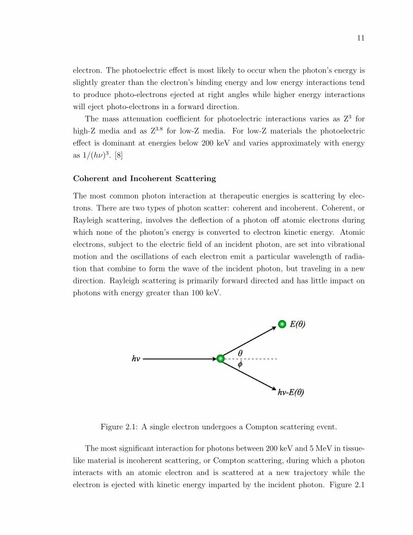
Figure 2.1: A single electron undergoes a Compton scattering event.

The most significant interaction for photons between 200 keV and 5 MeV in tissue-

like material is incoherent scattering, or Compton scattering, during which a photon

interacts with an atomic electron and is scattered at a new trajectory while the

electron is ejected with kinetic energy imparted by the incident photon. Figure 2.1

12

shows a schematic of a Compton scattering event. The photon has initial energy hν

before colliding with the electron. Because the electron’s binding energy is greatly

exceeded by the energy of the incident photon, it is treated as a free electron. The

electron is ejected from its orbit at some angle θ with energy E(θ) while the photon

is scattered at a corresponding angle φ with energy hν − E(θ).

The Klein-Nishina formula is used by EGSnrc Monte Carlo, discussed in Section

3.1, to determine the Compton cross section and is given per unit solid angle:

dσ

dΩ=r202

(1 + cos2 θ

) 1

1 + α(1− cos θ)

21 +

α2(1− cos θ)2

[1 + α(1− cos θ)](1 + cos2 θ)

(2.1)

where α = hν/m0c2, and m0c

2 is the rest mass of an electron. [8]

If the scattered electron is emitted in the direction of the incident photon, the

scattered photon will be emitted at 180 and the electron will have the maximum

energy possible for a Compton electron. Conversely, a scattered electron will receive

the least possible energy if the incident photon grazes by and continues nearly straight

forward, emitting the scattered electron at nearly 90. Compton interactions are

nearly independent of atomic number and decrease with increasing energy. [8]

Pair Production

Pair production is the conversion of energy to mass that results when a photon is

subject to the strong field of an atomic nucleus and becomes an electron-positron

pair. The photon must have energy of at least 1.022 MeV to comprise the rest masses

of the charged particles. Any additional energy held by the photon is distributed

between the electron and positron as kinetic energy. Because the atomic nucleus plays

a part in this interaction it receives a very small portion of the photon’s momentum;

consequently, the momentum of the electron does not uniquely predict the momentum

of the positron and vice-versa. If the incident photon has an energy of at least 2.04

MeV, it may interact in the field of an orbital electron to the same end, with the

addition of an ejected atomic electron. This less common process is called triplet

production as it produces a total of three charged particles.

A positron will propagate through and ionize matter in the same manner as an

electron until it slows enough to annihilate with a free electron and produce two 0.511

MeV photons which are ejected at 180 from one another. If the positron has some

13

remaining kinetic energy when it annihilates, the angle will be nearly 180.

The incidence of pair-production interactions increases rapidly with increasing

energy once the 1.022 MeV threshold has been met and the mass attenuation coeffi-

cient increases approximately with atomic number. Pair production is the dominant

photon interaction at energies in excess of 5 MeV. [8]

Characteristic x-rays & Auger Electrons

Characteristic x-rays, or fluorescence x-rays, are the photons emitted when an atomic

orbital vacancy is filled by an electron from a higher orbital shell. The energy of a

characteristic x-ray is equal to the difference in binding energies between the orbital

levels and is unique to atomic number. If a characteristic x-ray is absorbed by an

outer orbit electron, that electron is ejected with the energy of the characteristic x-ray

less the binding energy of the electron and is called an Auger electron. [8]

2.1.2 Electron Interactions

The dose perturbations of interest in this work are due, primarily, to the increase in

number and scattering of secondary electrons [17]. Electron interactions, including

radiative scattering, are covered here.

Soft & Hard Collisions

By convention, when an electron interacts with another electron it is assumed that the

electron that emerges with the greatest energy is the original electron: the maximum

energy transfer between electrons is half the incident energy. An electron-electron

interaction is depicted in Figure 2.2. As a free electron approaches a bound electron

their fields interact causing the bound electron to become excited or even ejected,

ionizing the atom [10].

The impact parameter, b, determines the magnitude of energy transfer from the

free electron to the bound electron. While b is greater than the atomic radius, r, the

transfer of energy is typically small and is inversely proportional to b2; this interaction

is called a soft collision [8]. When b is approximately r, however, large energy transfers

occur as the electrons collide and the binding energy of the atomic electron is negligible

[18]. These high energy interactions are called hard collisions and their resulting

secondary electrons are referred to as delta rays [10].

14

Figure 2.2: Schematic depiction of a soft electron interaction with another electron.

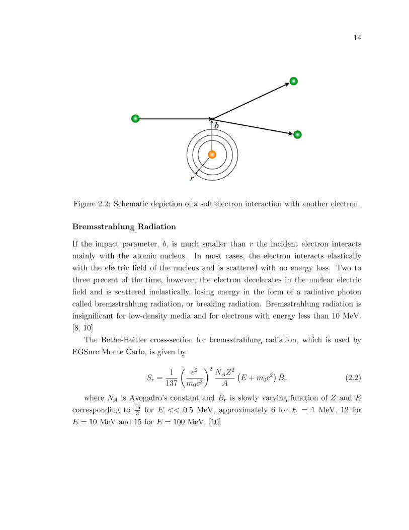
Bremsstrahlung Radiation

If the impact parameter, b, is much smaller than r the incident electron interacts

mainly with the atomic nucleus. In most cases, the electron interacts elastically

with the electric field of the nucleus and is scattered with no energy loss. Two to

three precent of the time, however, the electron decelerates in the nuclear electric

field and is scattered inelastically, losing energy in the form of a radiative photon

called bremsstrahlung radiation, or breaking radiation. Bremsstrahlung radiation is

insignificant for low-density media and for electrons with energy less than 10 MeV.

[8, 10]

The Bethe-Heitler cross-section for bremsstrahlung radiation, which is used by

EGSnrc Monte Carlo, is given by

Sr =1

137

(e2

m0c2

)2NAZ

2

A

(E +m0c

2)Br (2.2)

where NA is Avogadro’s constant and Br is slowly varying function of Z and E

corresponding to 163

for E << 0.5 MeV, approximately 6 for E = 1 MeV, 12 for

E = 10 MeV and 15 for E = 100 MeV. [10]

15

2.2 Dose Calculation Algorithms

Historically, dose computation algorithms have been either correction-based or model-

based. Correction-based algorithms start with the distribution of dose delivered to

a phantom and require corrections for contour irregularities, media inhomogeneities,

beam modifiers and variations in the distance from the beam source [5]. These cal-

culations can be done largely by hand, and while they are useful for making ballpark

estimates of dose distributions, they are no longer used for clinical treatment planning

if model-based algorithms are available.

Model-based algorithms simulate dose deposition based on the actual volume of

interest, usually a patient CT [5]. Having potential for greater accuracy and expedi-

ency resulting from the use of a computer, model-based algorithms are the standard

technique for performing treatment planning calculations. The algorithms of conse-

quence to this work can be subdivided into convolution-superposition algorithms and

Boltzmann-solvers, described below.

2.2.1 Convolution-Superposition Algorithms

Convolution algorithms model dose deposition in a two step process. In the first step,

primary photons are transported to their first interaction site where TERMA, or total

energy released per unit mass, is assigned. TERMA is the product of the primary

energy fluence and the mass attenuation coefficient for the material of interest. In

the second step, a convolution kernel is applied to model the dose scatter that results

from secondary photon and electron intereactions. The resulting dose, D (~r), is a

convolution of the TERMA, T , and a dose kernel, A,

D(~r) = T ∗ A. (2.3)

A dose kernel is a matrix that represents dose deposition by scattered photons

and electrons generated by the initial interactions of primary photons. The kernel

can be generated by measurement or by a modeling system such as Monte Carlo. A

convolution-superposition employs a number of dose kernels that have been measured

for various materials or modified for radiological path length using an electron-density

specific scaling factor. A linear combination of each dose kernel convolution makes

up the final result. Because the propagation of secondary photons and electrons

is measured or modeled ahead of time, convolution and convolution-superposition

16

algorithms are characteristically fast. [5, 19]

AAA

The anisotropic analytical algorithm, or AAA, is the convolution-superposition al-

gorithm currently used at VIC for modeling most radiotherapy plans. It uses linear

combinations of mono-energetic dose spread kernels, generated by EGSnrc Monte

Carlo, to separately model lateral and depth scatter for primary photons, extra-focal

photons and contaminant electrons before summing their contributions. Electron-

density scaling factors are used to account for inhomogeneities in the lateral direction

while a one-dimensional scatter kernel is employed along the depth axis to account

for material interfaces. AAA has shown improved accuracy over its predecessors and

good performance for most clinical applications. [15, 20]

2.2.2 Linear Boltzmann Transport Equation

The Linear Boltzmann Transport Equation is a differential equation or set of partial

differential equations that govern the evolution of spatial and energy distributions of a

population of particles [21]. For radiation therapy planning purposes the distribution

of ionizing particles is of interest, so the LBTE takes the form of the partial differential

equations

Ω · ~∇Φγ + σγt Φγ = qγγ + qeγ + qγ, (2.4)

Ω · ~∇Φe + σetΦe − ∂

∂E(SRΦe) = qee + qγe + qe. (2.5)

Equation 2.4 describes photon (γ) transport while equation 2.5 describes electron

(e) transport. Φγ(~r, E, Ω) and Φe(~r, E, Ω) are the photon and electron angular fluence,

respectively, ~r is a position vector, E is energy of the particle and Ω is the unit

direction vector. σγt (r, E) and σet (~r, E) are total photon and electron cross sections,

respectively, and SR (~r, E) is the restricted collisional and radiative stopping power,

representing the continuous slowing down operator. The terms on the right hand

side of equations (2.4) and (2.5) are primary and scatter source terms. qγ and qe

are primary photon and electron source terms, respectively, qγγ represents scattered

photons due to photon interactions, qee represents scattered electrons due to electron

interactions, qeγ represents scattered photons due to electron interactions and qγe

17

represents the reverse. [3]

Once Equations 2.4 and 2.5 are solved for electron fluence, the dose deposited at

any given point can be found as the product of the local electron fluence and material

specific stopping power:

D =

∫ ∞0

ΦeSRdE. (2.6)

Monte Carlo provides a stochastic solution to the LBTE while Acuros XB solves

these equations deterministically using an iterative approach. Both approaches are

summarized below.

Monte Carlo

Monte Carlo simulations are stochastic solutions to the LBTE. A random number

generator is used to sample the properties and interactions of single particles. These

properties and interactions are stored in particle histories and accumulated over mil-

lions of particles to obtain a single solution; the more particles simulated, the less

noise or variance present in the solution [5]. Particle interactions are modeled using

fundamental physics principles and so, Monte Carlo solution accuracy is limited by

the finite number of particles simulated and by uncertainty in user input rather than

approximation of the physics [3].

The computation time required to simulate millions or billions of individual par-

ticles is appreciable: on the order of hours to days. For example, an open 18 MV

field incident on an average patient sized phantom can take as long as 39 hours on

a cluster of 36 1.8 GHz CPUs. To improve calculation efficiency, a number of stan-

dard approximations are made which contribute as little as possible to the overall

systematic uncertainty. One such approximation is multiple scattering, a process by

which many electron interactions, both elastic and inelastic, are treated as a single

cumulative interaction or condensed history. This is done by sampling predetermined

scatter or energy-loss distributions, and results in more efficient electron transport

[22]. Other approximations vary by platform or by user preference and will be dealt

with in Chapter 3.

18

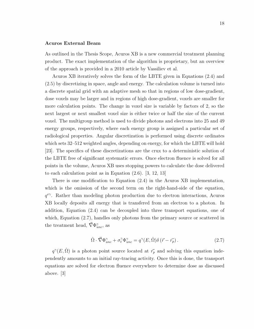
Acuros External Beam

As outlined in the Thesis Scope, Acuros XB is a new commercial treatment planning

product. The exact implementation of the algorithm is proprietary, but an overview

of the approach is provided in a 2010 article by Vassiliev et al.

Acuros XB iteratively solves the form of the LBTE given in Equations (2.4) and

(2.5) by discretizing in space, angle and energy. The calculation volume is turned into

a discrete spatial grid with an adaptive mesh so that in regions of low dose-gradient,

dose voxels may be larger and in regions of high dose-gradient, voxels are smaller for

more calculation points. The change in voxel size is variable by factors of 2, so the

next largest or next smallest voxel size is either twice or half the size of the current

voxel. The multigroup method is used to divide photons and electrons into 25 and 49

energy groups, respectively, where each energy group is assigned a particular set of

radiological properties. Angular discretization is performed using discrete ordinates

which sets 32–512 weighted angles, depending on energy, for which the LBTE will hold

[23]. The specifics of these discretizations are the crux to a deterministic solution of

the LBTE free of significant systematic errors. Once electron fluence is solved for all

points in the volume, Acuros XB uses stopping powers to calculate the dose delivered

to each calculation point as in Equation (2.6). [3, 12, 13]

There is one modification to Equation (2.4) in the Acuros XB implementation,

which is the omission of the second term on the right-hand-side of the equation,

qeγ. Rather than modeling photon production due to electron interactions, Acuros

XB locally deposits all energy that is transfered from an electron to a photon. In

addition, Equation (2.4) can be decoupled into three transport equations, one of

which, Equation (2.7), handles only photons from the primary source or scattered in

the treatment head, ~∇Φγunc, as

Ω · ~∇Φγunc + σγt Φγ

unc = qγ(E, Ω)δ (~r − ~rp) . (2.7)

qγ(E, Ω) is a photon point source located at ~rp and solving this equation inde-

pendently amounts to an initial ray-tracing activity. Once this is done, the transport

equations are solved for electron fluence everywhere to determine dose as discussed

above. [3]

19

2.3 Imaging and Contouring

Both medical images and radiation dose distributions are reported in a medical image

format called DICOM. DICOM stands for Digital Imaging and Communications in

Medicine and provides a standard format for the storage and transfer of clinical data

such as diagnostic or planning images [24]. When dealing with image or dose files in

this work, the files are in DICOM format.

2.3.1 Computed Tomography & Hounsfield Unit Saturation

Computed tomography, or CT, is the imaging modality used most often for radiation

therapy treatment planning. An x-ray source mounted on a rotating gantry opposite a

series of detectors moves around a patient taking a series of images at regular angular

intervals. The attenuation of the x-ray beam measured at each angle is backprojected

and processed to reproduce an attenuation map. As the patient is moved through the

gantry, attenuation is measured along the length of the body, producing a 3D image.

[24]

Each pixel of a CT image is represented by an integer called a Hounsfield Unit

(HU). Hounsfield Units correspond to the linear attenuation of photons with an av-

erage energy of 75 keV by a material, compared to the attenuation of water [24]. For

a voxel (x, y, z),

HU(x, y, z) = 1000µ(x, y, z)− µwater

µwater. (2.8)

Each CT imager has a fixed range of possible HU values and a unique linear

piecewise conversion curve between HU and density, so a single treatment planning

system may contain CT conversion data for multiple imagers. CT-saturation occurs

when the imaging unit attempts to scan an object with density exceeding the scanner’s

range. These regions are assigned the highest available HU value, and so, density-

specific information is lost. In addition, the presence of high density materials may

result in total attenuation of the x-ray beam which is not processed normally by the

backprojection algorithm and produces streaking, shadowing and blurring artifacts.

In-house artifact suppression algorithms and complementary megavolt imaging have

been explored as techniques for reducing high-density generated artifacts [25, 26].

Presently, however, these techniques are not widely used or easily integrated into the

workflow of a busy clinic, and they are not immediately available at VIC.

20

2.3.2 Pixelation

Picture and volume elements, pixels and voxels, respectively, have a finite minimum

size that determines the resolution of an image or dose distribution. This means that

data that exist or events that occur over distances smaller than the pixel or voxel

size may be lost through averaging necessitated by assigning one set of data to each

image or dose element.

As well, depending on the display system interpreting the DICOM, the location

of a pixel or voxel may be offset by up to a whole pixel or voxel width. For example,

in a 2-D case, suppose one system interprets the image or dose information assigned

to a pixel to correspond spatially to the top left corner of the pixel while another

interprets the data to correspond to the center of the pixel. The result is two in-

terpretations of the same data with a half pixel offset in the x- and y-directions as

shown in Figure 2.3. Variations in spatial interpretation must be considered, along

with volume averaging effects, when interpreting DICOM results.

x= 0 1

y=

0

1

x= 0 1

y=

0

1

Figure 2.3: A single 2-D data set can be interpreted in a number of ways. Top:Spatial information is assigned to the top left corner of the pixel. Bottom: Spatialinformation is assigned to the centre of the pixel.

21

2.3.3 Contouring

In planning radiation therapy treatments, dosimetrists, oncologists and physicists

evaluate the dose delivered to specific volumes such as the tumour mass and critical

organs. To facilitate this, treatment planning systems provide tools to delineate each

of these volumes with a structure called a contour. Contours can be either hand

drawn or automatically created by the treatment planning system, and are not only

useful for evaluation purposes, but also for optimization algorithms where a conformal

dose to some volume can be weighted against the sparing of another. In the case of

erroneous HU assignment, contouring can be used to reassign appropriate material

properties, including properties for materials beyond the HU range of the CT scanner.

This is a useful tool when assigning material properties to high-density implants, but

CT saturation is usually accompanied by an increase in image artifacts, as well as

blurring of the object’s dimensions, which are not as easily corrected.

Contouring has some important limitations, the foremost being the pixelation ef-

fects discussed in the previous section. In addition, some treatment planning systems,

such as Eclipse, use vector based contours and there is uncertainty as to how pixels

along the contour-boundary are assigned. In this research it has been observed that

vector contours are not ideal for handling sharp angles and that synthetic volumes

with sharp angles are not contoured accurately. Overall, it should be emphasized

that contours are virtual structures superimposed onto CT density maps as tools

with associated uncertainties.

2.4 Radio-chromic Film

A set of experimental measurements to be introduced in Chapter 3 were performed

using radio-chromic film, a radiation-sensitive film used in relative dosimetry. Its

properties are closer to tissue than silver-based films, and unlike the dedicated wet

labs required for chemical processing of silver-based films, radio-chromic film is self-

developing. In addition, radio-chromic film is insensitive to visible light, making it

easy to handle. Because of these advantages and its continuing improvements in

performance, radio-chromic film is gradually replacing silver-based film in dosimetric

and diagnostic applications.

Generally, radio-chromic film consists of an active layer of photomonomer molecules

mounted on a polyester base. When exposed to radiation, the photomonomer molecules

22

are excited by photons, electrons, or other energetic molecules, and this produces a

chemical change resulting in a colour change. The film requires only a few milliseconds

to develop, but may require up to an hour to become chemically stable, so reading

usually takes place after some time period as recommended by the manufacturer. [27]

As a relative dosimeter, radio-chromic film must be calibrated before it can be

used for measurements. This can be done by delivering a known range of doses to

film from the batch to be used in the measurements, taking care to keep a sample

unirradiated for a 0 Gy fog and base reading. These calibration measurements can

be used to create an optical density (OD) to dose conversion curve. Optical density

is a measure of light transmission and is given by

OD = log10

(I0I

)(2.9)

where I0 is the initial light intensity and I is the transmitted light intensity. A

densitometer is used to measure OD by directly measuring transmitted light through

a sample and comparing with the known intensity of the light source. Because radio-

chromic film has some directional dependance, film orientation should be noted and

consistent through the calibration, measurement and readout process. Once the cal-

ibration curve is established, additional films can be irradiated and their measured

OD converted to dose. [24]

2.5 Summary

Chapter 2 has covered photon and electron interactions at therapeutic energies, radio-

therapy modeling techniques, CT imaging and processing for radiotherapy planning,

and the properties and use of radio-chromic film for relative dosimetry. In Chapter

3, these ideas are applied to experimental measurements and calculations to enable

an evaluation of Acuros XB as applied to radiotherapy planning around high-density

implants.

23

Chapter 3

Methods & Materials

In order to evaluate Acuros XB for dose calculations involving high-density pertur-

bations using Monte Carlo as the reference, the parameters of the dose calculation

algorithms must be understood and matched as closely as possible. Chapter 3 summa-

rizes the modeling parameters used and approximations made by Acuros XB, EGSnrc

Monte Carlo and AAA. The experimental measurements and calculations performed

are also outlined, as well as some of the evaluation techniques used to analyze the

results.

3.1 Modeling Environments & Parameters

3.1.1 Introduction

Monte Carlo

All of the Monte Carlo modeling in this work was done using BEAMnrc and DOSXYZnrc

which are built on the EGSnrc code system [28]. BEAMnrc models beam production,

shaping and transport through the linear accelerator while DOSXYZnrc transports

the resulting particle histories through a patient or phantom geometry in order to

score dose deposition [29, 30]. The patient or phantom geometry is generated by a

program called ctcreate which reads a set of CT DICOM files and converts the data

into a file containing spatial, material and density information that is useable by the

EGSnrc system. The conversion from HU to material and density values is user de-

fined and will be discussed further in Section 3.1.3. Thirty-six 1.8 GHz CPUs housed

in three computer nodes comprise the Beowulf cluster that runs Monte Carlo calcula-

24

tions at VIC. The cluster was set up and is run on a front end node by Rocks Cluster

Distribution from National Partnership for Advanced Computational Infrastructure

while the workload is managed by Condor. User input is done through a web-based

application networked through the front end node.

The BEAMnrc and DOSXYZnrc code systems are widely used and trusted for

benchmarking, and the VIC implementation is no exception [3, 13, 14, 15, 31]. For this

reason, Monte Carlo solutions will be used as the reference in calculation comparisons

throughout this work.

Eclipse

Eclipse is the commercial treatment planning software package distributed by Varian

Medical Systems that is used at VIC and in this work. Eclipse provides a single user

interface for a number of calculation algorithms including pencil beam convolutions,

AAA and most recently, Acuros XB. The system provides a graphical user interface for

contouring structures and planning treatment fields on a 3D planning image, usually

a CT DICOM set. As well, the program provides an environment for comparing

plans and dose distributions. Some Eclipse features are shared between AAA and

Acuros XB while others are specific to each algorithm. In the following discussion of

modeling parameters, when a feature applies to both algorithms it will be discussed

under the heading Eclipse, otherwise, it will be discussed under the headings AAA

and Acuros XB.

3.1.2 Source Model

Monte Carlo

The radiation source model generated by BEAMnrc has been tuned to match the out-

put of the Varian Clinac R© 21EX linear accelerators used for radiation therapy treat-

ment at VIC. Electrons and photons are transported through the explicitly modeled

internal structure of the linear accelerator head to produce a phase space that defines

the position, direction, energy and charge information of each photon or electron that

crosses a particular spatial plane of the model. At VIC, output models have been

created for 18 and 6 MV spectral photons, both of which are used in the experimental

calculations to follow.

25

Eclipse

Eclipse provides the same radiation source model for Acuros XB and AAA calcula-

tions. The source model has also been tuned to match the output of a Varian Clinac

21EX linear accelerator using a proprietary configuration algorithm that modifies pa-

rameter values until the modeled output matches set of beam measurements provided

by the user, including profiles and depth doses for various field sizes. Again, output

models have been configured for 18 and 6 MV spectral photon beams.

3.1.3 Material Data

For EGSnrc Monte Carlo and Eclipse, material and density assignment is performed

according to a user defined HU to density conversion curve which is specific to the

CT imager used to acquire the planning image. For this research, the curves had to

be artificially extended to include titanium alloy and stainless steel by adding points

to the conversion curve beyond 4000 HU and 4.0 g/cm3. The resulting conversion

curves are shown in Figure 3.1 and the properties of stainless steel and titanium alloy

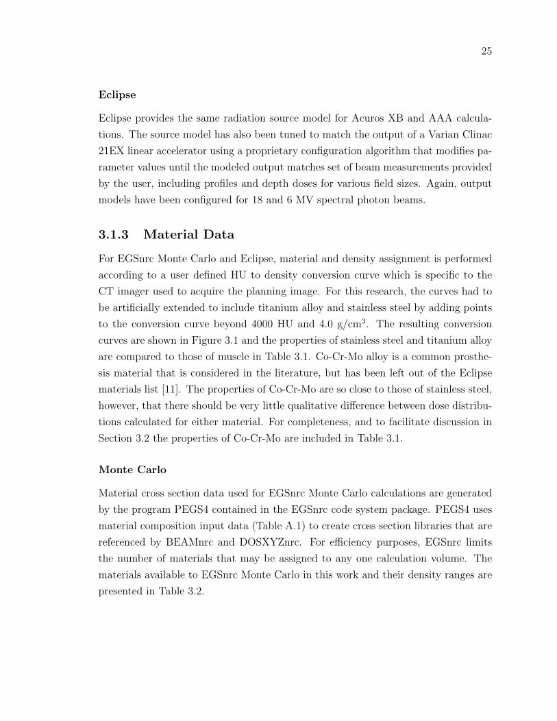
are compared to those of muscle in Table 3.1. Co-Cr-Mo alloy is a common prosthe-

sis material that is considered in the literature, but has been left out of the Eclipse

materials list [11]. The properties of Co-Cr-Mo are so close to those of stainless steel,

however, that there should be very little qualitative difference between dose distribu-

tions calculated for either material. For completeness, and to facilitate discussion in

Section 3.2 the properties of Co-Cr-Mo are included in Table 3.1.

Monte Carlo

Material cross section data used for EGSnrc Monte Carlo calculations are generated

by the program PEGS4 contained in the EGSnrc code system package. PEGS4 uses

material composition input data (Table A.1) to create cross section libraries that are

referenced by BEAMnrc and DOSXYZnrc. For efficiency purposes, EGSnrc limits

the number of materials that may be assigned to any one calculation volume. The

materials available to EGSnrc Monte Carlo in this work and their density ranges are

presented in Table 3.2.

26

Table 3.1: Material properties for muscle, titanium, stainless steel and Co-Cr-Mo[8, 11].

Material Muscle Titanium Stainless Steel Co-Cr-Mo

Mass Density1.04 4.3 8.1 7.9

(g/cm3)Electron Density

3.4× 1023 1.2× 1024 2.3× 1024 2.2× 1024

(e−/cm3)Effective Atomic

7.64 21.4 26.7 27.6Number

Eclipse

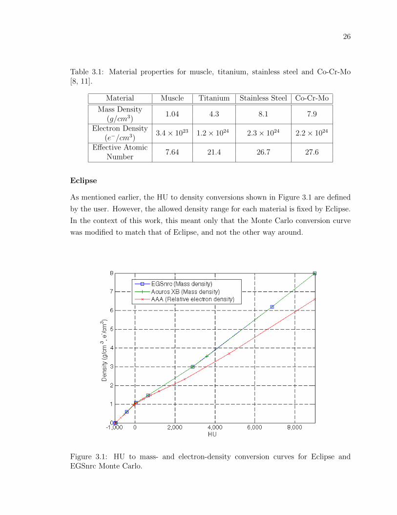
As mentioned earlier, the HU to density conversions shown in Figure 3.1 are defined

by the user. However, the allowed density range for each material is fixed by Eclipse.

In the context of this work, this meant only that the Monte Carlo conversion curve

was modified to match that of Eclipse, and not the other way around.

Figure 3.1: HU to mass- and electron-density conversion curves for Eclipse andEGSnrc Monte Carlo.

27

Acuros XB includes an important high-density material assignment restriction:

any voxel containing an HU value that corresponds to a density greater than 3.0 g/cm3

must be included in a structure and assigned a specific material or the calculation will

be prevented from proceeding. The partial inclusion of high density voxels by vector-

based contours means that contours defining high-density structures often require

an external margin of 0.1 cm, as recommended by Varian, to encompass the entire

object. This artificially inflates the size of the structure, but is necessary to proceed

with the calculation.

Table 3.2: Materials and corresponding density ranges for Eclipse and EGSnrc MonteCarlo.

Eclipse Monte Carlo

MaterialMin ρ Max ρ

MaterialMin ρ Max ρ

(g/cm3) (g/cm3)

Air 0.0010 0.0112 Air 0.0 0.0114Lung 0.0010 0.5896 Lung 0.0114 0.5896

Adipose 0.5907 0.9849Muscle 0.5896 1.0748

Muscle 0.9853 1.0748Cartilage 1.0758 1.4749 Light Bone 1.0748 1.4749

Bone 1.4755 2.9997Bone 1.4749 2.9997

Aluminum 2.2754 3.5600Titanium Alloy 3.5600 6.2096 Titanium Alloy 2.9997 6.2096Stainless Steel 6.2104 8.0 Stainless Steel 6.2096 8.0

3.1.4 Interactions & Approximations

Monte Carlo

In VIC’s implementation of the code, EGSnrc models the photoelectric effect, Comp-

ton scattering, pair-production, positron annihilation and bremsstrahlung radiation.

It takes relativistic spin effects into account for electron transport and multiple scat-

tering is used for more efficient charged particle propagation [22]. For efficiency,

Rayleigh scattering is not modeled and characteristic x-rays are handled only approx-

imately: for a photoelectric interaction, the energy that would be lost to overcome

binding energy and then emitted during atomic relaxation is transferred entirely to

the photoelectron. Bethe-Heitler cross-sections are used for bremsstrahlung radia-

tion, the Klein-Nishina formula determines Compton scattering cross-sections and

28

photoelectrons inherit the direction of incident photons. [29]

The parameter ECUT, electron cutoff energy, defines the energy at which it is

assumed that an electron will not be capable of leaving the current voxel and its

remaining energy deposited locally. The default value of ECUT is 0.7 MeV for a

remainder electron energy of 0.189 MeV after subtracting the electron rest mass,

0.511 MeV. To be sure that this parameter was appropriate for high density-gradient

scenarios, calculations were performed using an ECUT value of 0.521 MeV for a

minimum electron energy of 0.010 MeV. Differences between the results were not

statistically significant, and the lower ECUT value almost doubled calculation time,

so ECUT = 0.7 MeV was used. [29]

Acuros XB

As discussed in Chapter 2, Acuros XB uses ray tracing to transport primary and scat-

tered source photons to the calculation volume, while charged particles are propagated

by solving Equations (2.4) and (2.5) with some physical approximations, listed here.

Both secondary charged particles produced in pair production are modeled as elec-

trons instead of one electron and one positron, and, as mentioned before, photons pro-

duced by electrons are not modeled explicitly. Instead, energy from bremsstrahlung

radiation and characteristic x-rays is deposited locally.

AAA

Chapter 2 discusses how AAA uses dose kernels and electron-density scaling to simu-

late dose scattered laterally from a ray of photons, and one-dimensional dose kernels

to deal with inhomogeneities with depth. As the dose kernels are generated using

EGSnrc Monte Carlo, AAA effectively models all of the interactions that EGSnrc

Monte Carlo models. However, the pre-calculated kernels are calculated for water

and scaled depending on the material of interest in the calculation volume. This

technique is insufficient when dealing with sharp dose perturbations due to a high-

density object . Consequently, throughout the experimental cases presented in the

following chapters AAA is not expected to accurately handle high-density dose per-

turbations. This is not meant to discredit AAA as a clinically useful algorithm, only

to highlight its limitations for one subset of clinical applications.

29

3.2 Experimental Measurements

As discussed in Chapter 2, the presence of a high-density object in a radiation field is

expected to increase secondary photon and electron scattering, resulting in elevated

dose at the entrance and lateral surfaces of the object while shadowing regions beyond

it. These perturbations are presented in Figure 1.5, which shows dose profile and

depth dose plots of EGSnrc Monte Carlo data for 18 MV photons through a phantom

with and without a high-density centre. A variation on this data was presented

in a 2003 Task Group Report of the American Association of Physicists in Medicine

(AAPM) that encompassed recommendations for treatment planning for patients with

hip prostheses. The Monte Carlo data presented in this document, generated by an

unspecified Monte Carlo system, has been reproduced with permission in Figure 3.2

and shows a 30% dose peak at the distal surface of a Co-Cr-Mo centre, allegedly

due to pair-production interactions within the metal [11]. This forward peak was not

seen in the EGSnrc Monte Carlo data used in this work, nor in Acuros XB results.

Consequently, a set of film measurements were performed to ascertain which model

is closest to reality.

Figure 3.2: Depth dose perturbation data included in AAPM TG Report 63 [11].Reproduced with permission from the AAPM.

30

Although the data presented in the Task Group Report was for 18 MV photons

through a Co-Cr-Mo slab, the measurements presented here were performed using

18 MV photons through a slab of steel with the same dimensions. The properties of

steel are close enough to Co-Cr-Mo that there should be no qualitative difference in

the dose distribution. The steel slab was placed between slabs of Solid Water R© with

sections of Gafchromic R© EBT2 radio-chromic film placed at intervals throughout.

Figure 3.3 shows the geometric setup used for the measurements. Arranging the

stack with the upper steel surface at isocenter, labeled with a red x, 5 cm Solid Water

was placed on top of the steel with film placed at 3.5 cm (dmax), 4.5 cm and 5.0 cm

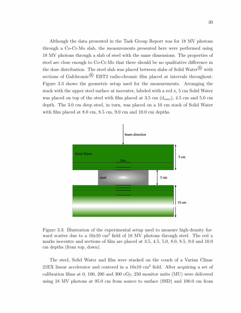
depth. The 3.0 cm deep steel, in turn, was placed on a 10 cm stack of Solid Water

with film placed at 8.0 cm, 8.5 cm, 9.0 cm and 10.0 cm depths.

Figure 3.3: Illustration of the experimental setup used to measure high-density for-ward scatter due to a 10x10 cm2 field of 18 MV photons through steel. The red xmarks isocentre and sections of film are placed at 3.5, 4.5, 5,0, 8.0, 8.5, 9.0 and 10.0cm depths (from top, down).

The steel, Solid Water and film were stacked on the couch of a Varian Clinac

21EX linear accelerator and centered in a 10x10 cm2 field. After acquiring a set of

calibration films at 0, 100, 200 and 300 cGy, 250 monitor units (MU) were delivered

using 18 MV photons at 95.0 cm from source to surface (SSD) and 100.0 cm from

31

Figure 3.4: Calibration curve for Gafchromic R© EBT2 radio-chromic dosimetric film.

source to the isocentre (SAD). The film was placed in an envelope and allowed to

stabilize before a MacBeth Process Measurements TD932 Densitometer was used to

measure the OD of each film. Eight measurements of OD were taken for each film

and used to calculated a mean value and standard deviation. The calibration curve,

fitted with a square root function, is shown in Figure 3.4. Error bars on each data

point are representative of the standard deviation of measured values.

A virtual phantom of the experimental setup was generated in Eclipse by creating

structures in an empty CT image and assigning appropriate material and density

properties. The Solid Water regions were assigned skeletal muscle with 0 HU contents

corresponding to 1.0 g/cm3 while steel was assigned stainless steel with 8999 HU

corresponding to 8.0 g/cm3. Acuros XB, AAA and EGSnrc Monte Carlo were then

used to calculate the depth doses expected from the film measurements. Acuros XB

and AAA data were calculated on a 0.1 cm voxel grid while EGSnrc Monte Carlo data

was calculated on a 0.2 cm voxel grid as 0.2 cm was the finest resolution available for

the size of CT image used.

32

3.3 Experimental Calculations

The primary method used for evaluating the accuracy of Acuros XB is comparison

with EGSnrc Monte Carlo simulations for a number of phantom geometries of varying

complexity. The evaluation starts with a high-density rectangular rod inside a skeletal

muscle cube, continues with a water tank containing high-density cylindrical rods

and prostheses, and concludes with a patient CT and clinical treatment plan. Monte

Carlo simulations were performed to 1-2% standard deviation: approximately 7×109

particles and 5× 109 particles for 18 MV and 6 MV fields respectively, except for the

clinical case where 3.5× 109 particles were simulated.

3.3.1 Virtual Phantoms

In order to reduce potential sources of variation, initial experimental calculations

were performed for virtual phantoms with regular geometries and sharp boundaries.

To construct these phantoms, empty CT DICOM image sets were modified using

Mathworks R© MATLAB R©, Natick, MA, USA, and imported into Eclipse. The re-

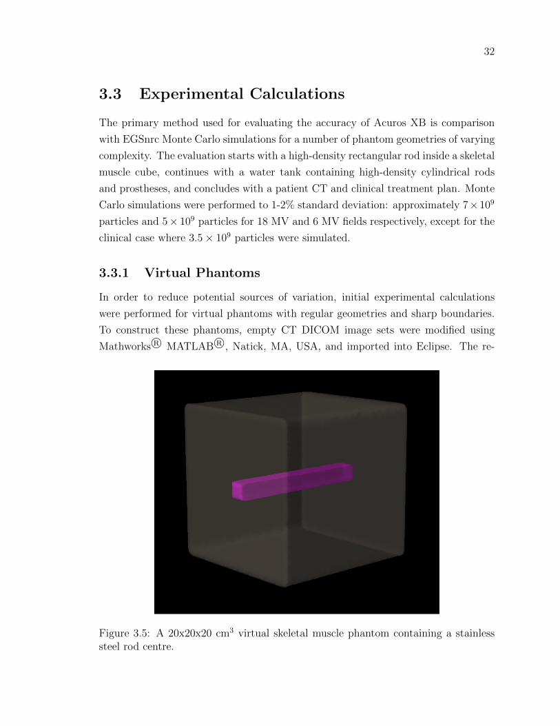
Figure 3.5: A 20x20x20 cm3 virtual skeletal muscle phantom containing a stainlesssteel rod centre.

33

sulting virtual phantoms are 20x20x20 cm3 and 10x10x10 cm3 skeletal muscle cubes,

each containing a stainless steel rod with a 2x2 cm2 square cross-section at its center,

oriented to be longest in the z-direction. Each slice has a resolution of 0.05 cm in

the x- and y-directions with slice thickness of 0.5 cm. A 3-D rendering of the larger

phantom is shown in Figure 3.5.

The high-density rod must be contoured and assigned a material in order for

Acuros XB to run, so it was possible to use the same phantoms for stainless steel,

titanium alloy and skeletal muscle internal structures by changing the material prop-

erties of the rod structure. Plans for these phantoms involved 10x10 cm2 and 5x5

cm2 fields focused on isocenter, both on-axis and at a 10 gantry angle using 18 and

6 MV photons.

3.3.2 Water Tank Phantoms

A water tank containing high density objects was scanned using a clinical CT unit

and loaded into Eclipse for planning and dose modeling. The water tank itself is

30x30x30 cm3 and is shown in Figure 3.8. For the scan, the tank was supported on 5

cm of Solid Water. Two plastic positioning guides were placed on the bottom of the

tank for reproducible setup and the tank was filled with water to the top of the blue

insert that can be seen at the top of Figure 3.8. A foam block, which is not shown in

the figure, was placed on top of the water to minimize motion during the CT scan.

Figure 3.6: Top: Stainless steel rod. Bottom left: Steel alloy hip prosthesis. Bottomright: Titanium alloy hip prosthesis.

34

Stainless Steel Rods

The first water tank geometry consists of two cylindrical stainless steel rods 20.32

cm (8 in) long and 2.54 cm (1 in) in diameter, shown in Figure 3.6 (top). The rods

were oriented on an angle of 10 and centered about 3.65 cm on either side of the

central beam axis. For calculation purposes, these rods were contoured as stainless

steel and subject to 10x10 cm2 fields of 18 MV and 6 MV photons delivered on axis.

The Eclipse-generated structure set for this phantom is shown in Figure 3.7.

Figure 3.7: Eclipse generated structure set for a plexiglass water tank containingcylindrical stainless steel rods.

Hip Prostheses

The second water tank geometry includes two hip prostheses, one a steel alloy and the

other a titanium alloy, both shown in Figure 3.6 (bottom). The exact properties of

the pieces are unknown, however, because their geometries are used only for computa-

tional purposes, throughout this work they are assumed to be solid. For calculations,

the prostheses are contoured as stainless steel and titanium alloy, respectively, and

subject to 10x10 cm2 fields of 18 MV and 6 MV photons. The Eclipse generated

structure set for this phantom geometry is shown in the bottom image of Figure 3.8.

35

Figure 3.8: Top: Water tank used for imaging steel rods and hip prostheses. The hipprostheses are shown in the positioning guides while the foam block is not shown.Bottom: Eclipse generated structure set for the plexiglass water tank containing thehip prostheses.

36

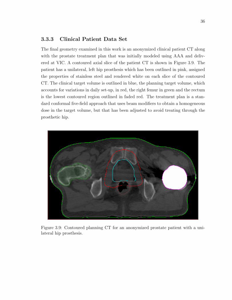
3.3.3 Clinical Patient Data Set

The final geometry examined in this work is an anonymized clinical patient CT along

with the prostate treatment plan that was initially modeled using AAA and deliv-

ered at VIC. A contoured axial slice of the patient CT is shown in Figure 3.9. The

patient has a unilateral, left hip prosthesis which has been outlined in pink, assigned

the properties of stainless steel and rendered white on each slice of the contoured

CT. The clinical target volume is outlined in blue, the planning target volume, which

accounts for variations in daily set-up, in red, the right femur in green and the rectum

is the lowest contoured region outlined in faded red. The treatment plan is a stan-

dard conformal five-field approach that uses beam modifiers to obtain a homogeneous

dose in the target volume, but that has been adjusted to avoid treating through the

prosthetic hip.

Figure 3.9: Contoured planning CT for an anonymized prostate patient with a uni-lateral hip prosthesis.

37

3.4 Reporting Methods

3.4.1 Profile & Depth Doses

In the presentation of data in Chapter 4 the terms dose profile and depth dose will be

used to describe plots. In all cases, a dose profile will refer to an array of data points

taken laterally from a single axial slice, perpendicular to the beam axis. Depth dose

will refer to an array of data points taken from a single axial slice in the direction of

the beam axis.

3.4.2 γ Evaluations

When dealing with large data sets involving high dose- and density-gradients within

complex geometries, such as human anatomy, it is usually impractical to compare dose

calculations voxel to voxel. A distribution with steep dose gradient and a single voxel

offset everywhere may represent the same dose deposition as a reference distribution,

but be evaluated as incorrect because of the offset. To address this, the concept of

distance to agreement has been integrated with percent dose difference to produce

the γ index, a radial measurement of the distance between agreeing dose points in

two distributions [32]. For a reference dose, Dref , at position rref and corresponding

analysis dose, Dc, at position rc, if the dose-difference and distance to agreement

criterion are ∆DM and ∆dM , respectively, the gamma index is defined as

γ(rref ) = min

√r2

∆d2M+

δ2

∆D2M

∀rc (3.1)

where

r = |rc − rref |, (3.2)

δ = Dc(rc)−Dref (rref ). (3.3)

If γ ≤ 1 then the evaluation passes, otherwise, if γ > 1 the evaluation fails. The

advantage of a γ-analysis over a point by point comparison is the allowance for spatial

or dose variations that result from averaging due to pixelation, variation in contour

interpretation and the presence of high dose- or density-gradients. In Chapter 4, γ-

evaluations will be performed to evaluate Acuros XB and AAA data against EGSnrc

Monte Carlo results for each of the calculations described in this chapter. Each 3D

matrix of γ-values will be reported as a percentage of voxels with γ ≤ 1, or within

38

tolerance.

39

Chapter 4

Results

Chapter 3 outlined experimental calculations performed for real and virtual phan-

toms, a prostate treatment plan for a patient with a unilateral hip prosthesis, and

film measurements undertaken to evaluate the distribution of dose on the distal in-

terface of a high-density region with Solid Water. The results of these calculations

and measurements are presented in the following chapter, beginning with film mea-

surement results. These are followed by a summary of the phantom and patient

calculations and a brief description of algorithm calculation times.

4.1 Film Measurements

Figure 4.1 presents the results of the film measurements described in Section 3.2.

Each data point represents the mean of eight OD measurements and the error-bars

represent the corresponding standard deviations. EGSnrc Monte Carlo, Acuros XB

and AAA were used to calculate the expected dose and are compared to the film

measurement data. The shape of the Monte Carlo depth dose data included in the

AAPM Task Group Report on planning for patients with hip prostheses, Figure 3.2,

suggests that there should be a forward scatter peak in excess of 30% on the distal

surface of the high-density inhomogeneity, however, neither the measured data, nor

the modeled data produces such a peak. Both Acuros XB and Monte Carlo outline

a build-up peak on the distal surface of the inhomogeneity due to reestablishment of

electron equilibrium, but this peak is on the order of 5%, much less than the 30% peak

presented in Figure 3.2. The film measurements confirm the absence of a dramatic

forward peak and reaffirm the validity of the data to be presented in the remainder

40

of this chapter, which are void of such a peak. [11]

The percent differences between measured and calculated data are also presented

in Figure 4.1. The large differences at 5.0 and 8.0 cm depths are likely due to uncer-

tainties in high-density boundary definition.

Figure 4.1: Film measurements and Acuros XB, AAA and EGSnrc Monte Carlodata for a 10x10 cm2 field of 18 MV photons through the high-density inhomogeneityoutlined in Figure 3.2. Percent differences between measured and calculated resultsare plotted in the lower portion of the graph. The solid black lines at 5 and 8 cmdepth indicate the steel boundaries.

4.2 Virtual Phantoms

20x20x20 cm3 Cubic Phantom

Figure 4.2 shows depth dose plots for a 10x10 cm2 field of 18 MV photons delivered

normal to the surface of the 20x20x20 cm3 virtual phantom described in Section 3.3.1

as calculated by Acuros XB, AAA and Monte Carlo. The dose grid has a resolution

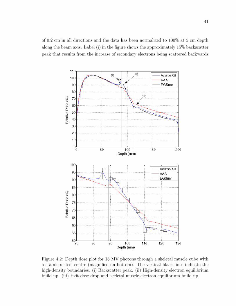
41

of 0.2 cm in all directions and the data has been normalized to 100% at 5 cm depth

along the beam axis. Label (i) in the figure shows the approximately 15% backscatter

peak that results from the increase of secondary electrons being scattered backwards

Figure 4.2: Depth dose plot for 18 MV photons through a skeletal muscle cube witha stainless steel centre (magnified on bottom). The vertical black lines indicate thehigh-density boundaries. (i) Backscatter peak. (ii) High-density electron equilibriumbuild up. (iii) Exit dose drop and skeletal muscle electron equilibrium build up.

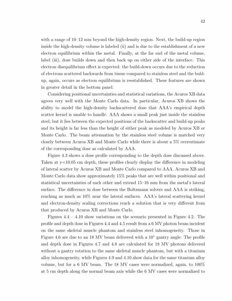
42

with a range of 10–12 mm beyond the high-density region. Next, the build-up region

inside the high-density volume is labeled (ii) and is due to the establishment of a new

electron equilibrium within the metal. Finally, at the far end of the metal volume,

label (iii), dose builds down and then back up on either side of the interface. This

electron disequilibrium effect is expected: the build-down occurs due to the reduction

of electrons scattered backwards from tissue compared to stainless steel and the buld-

up, again, occurs as electron equilibrium is reestablished. These features are shown

in greater detail in the bottom panel.

Considering positional uncertainties and statistical variations, the Acuros XB data

agrees very well with the Monte Carlo data. In particular, Acuros XB shows the

ability to model the high-density backscattered dose that AAA’s empirical depth

scatter kernel is unable to handle. AAA shows a small peak just inside the stainless

steel, but it lies between the expected positions of the backscatter and build-up peaks

and its height is far less than the height of either peak as modeled by Acuros XB or

Monte Carlo. The beam attenuation by the stainless steel volume is matched very

closely between Acuros XB and Monte Carlo while there is about a 5% overestimate

of the corresponding dose as calculated by AAA.

Figure 4.3 shows a dose profile corresponding to the depth dose discussed above.

Taken at y=10.05 cm depth, these profiles clearly display the difference in modeling

of lateral scatter by Acuros XB and Monte Carlo compared to AAA. Acuros XB and

Monte Carlo data show approximately 15% peaks that are well within positional and

statistical uncertainties of each other and extend 15–16 mm from the metal’s lateral

surface. The difference in dose between the Boltzmann solvers and AAA is striking,

reaching as much as 10% near the lateral surfaces. AAA’s lateral scattering kernel

and electron-density scaling corrections reach a solution that is very different from

that produced by Acuros XB and Monte Carlo.

Figures 4.4 – 4.10 show variations on the scenario presented in Figure 4.2. The

profile and depth dose in Figures 4.4 and 4.5 result from a 6 MV photon beam incident

on the same skeletal muscle phantom and stainless steel inhomogeneity. Those in

Figure 4.6 are due to an 18 MV beam delivered with a 10 gantry angle. The profile

and depth dose in Figures 4.7 and 4.8 are calculated for 18 MV photons delivered

without a gantry rotation to the same skeletal muscle phantom, but with a titanium

alloy inhomogeneity, while Figures 4.9 and 4.10 show data for the same titanium alloy

volume, but for a 6 MV beam. The 18 MV cases were normalized, again, to 100%

at 5 cm depth along the normal beam axis while the 6 MV cases were normalized to

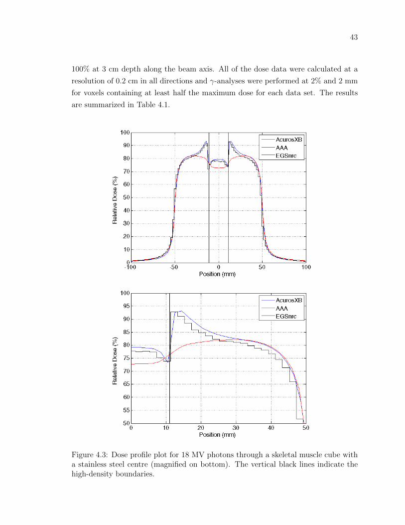
43

100% at 3 cm depth along the beam axis. All of the dose data were calculated at a

resolution of 0.2 cm in all directions and γ-analyses were performed at 2% and 2 mm

for voxels containing at least half the maximum dose for each data set. The results

are summarized in Table 4.1.

Figure 4.3: Dose profile plot for 18 MV photons through a skeletal muscle cube witha stainless steel centre (magnified on bottom). The vertical black lines indicate thehigh-density boundaries.

44

Figure 4.4: Depth dose plot for 6 MV photons through a 20x20x20 cm3 skeletalmuscle cube with a stainless steel centre (magnified on bottom). The vertical blacklines indicate the high-density boundaries.

45

Figure 4.5: Dose profile plot for 6 MV photons through a 20x20x20 cm3 skeletalmuscle cube with a stainless steel centre (magnified on bottom). The vertical blacklines indicate the high-density boundaries.

46

Figure 4.6: Depth dose (top) and dose profile (bottom) for 18 MV photons with a 10

gantry rotation through a 20x20x20 cm3 skeletal muscle cube with a stainless steelcentre. The vertical black lines indicate the high-density boundaries.

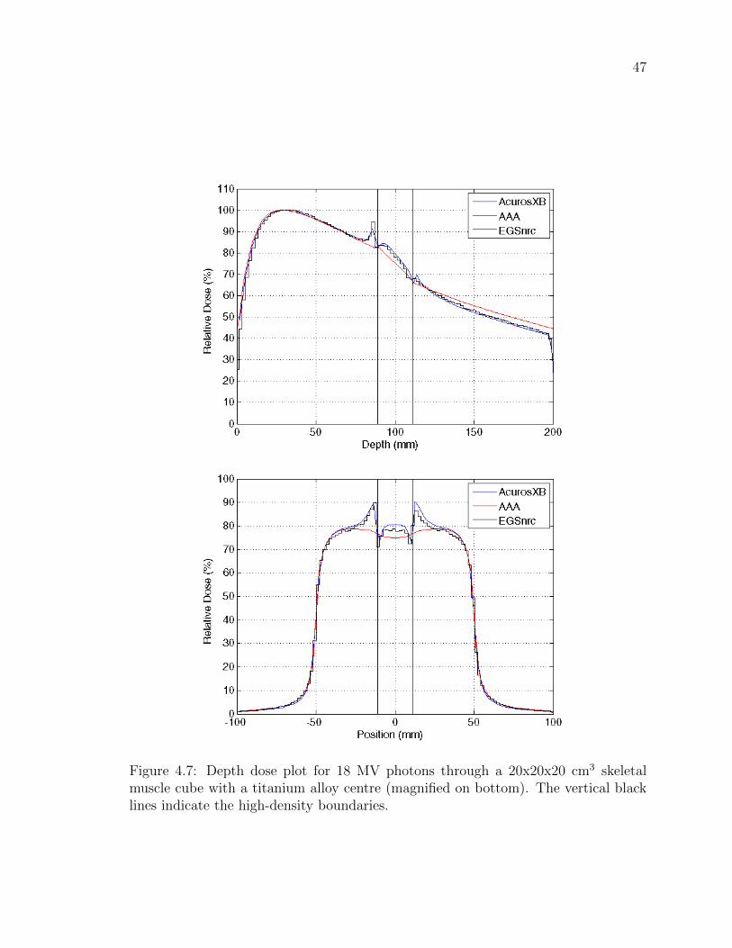
47

Figure 4.7: Depth dose plot for 18 MV photons through a 20x20x20 cm3 skeletalmuscle cube with a titanium alloy centre (magnified on bottom). The vertical blacklines indicate the high-density boundaries.

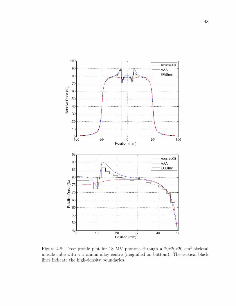
48

Figure 4.8: Dose profile plot for 18 MV photons through a 20x20x20 cm3 skeletalmuscle cube with a titanium alloy centre (magnified on bottom). The vertical blacklines indicate the high-density boundaries.

49

Figure 4.9: Depth dose plot for 6 MV photons through a 20x20x20 cm3 skeletal musclecube with a titanium alloy centre (magnified on bottom). The vertical black linesindicate the high-density boundaries.

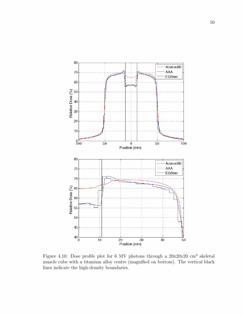
50

Figure 4.10: Dose profile plot for 6 MV photons through a 20x20x20 cm3 skeletalmuscle cube with a titanium alloy centre (magnified on bottom). The vertical blacklines indicate the high-density boundaries.

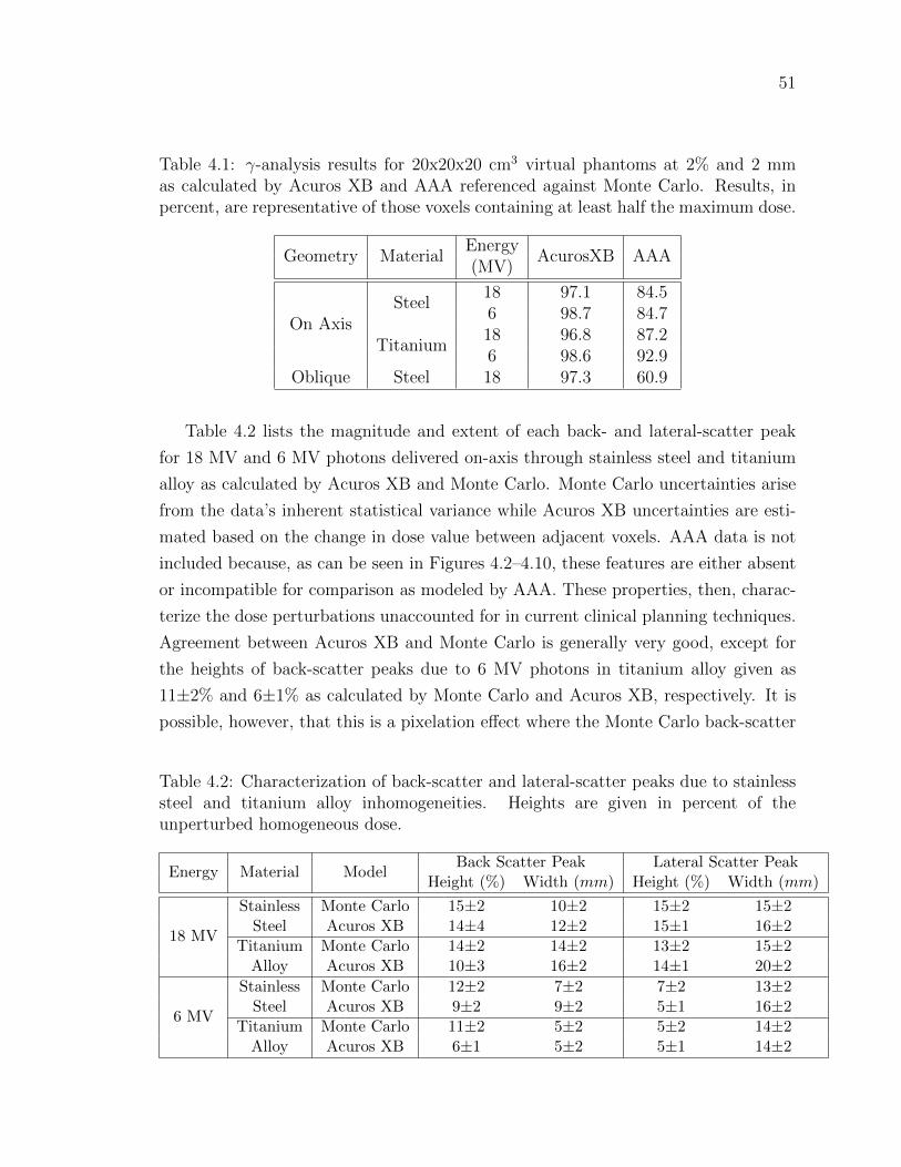
51

Table 4.1: γ-analysis results for 20x20x20 cm3 virtual phantoms at 2% and 2 mmas calculated by Acuros XB and AAA referenced against Monte Carlo. Results, inpercent, are representative of those voxels containing at least half the maximum dose.

Geometry MaterialEnergy

AcurosXB AAA(MV)

On AxisSteel

18 97.1 84.56 98.7 84.7

Titanium18 96.8 87.26 98.6 92.9

Oblique Steel 18 97.3 60.9

Table 4.2 lists the magnitude and extent of each back- and lateral-scatter peak

for 18 MV and 6 MV photons delivered on-axis through stainless steel and titanium

alloy as calculated by Acuros XB and Monte Carlo. Monte Carlo uncertainties arise

from the data’s inherent statistical variance while Acuros XB uncertainties are esti-

mated based on the change in dose value between adjacent voxels. AAA data is not

included because, as can be seen in Figures 4.2–4.10, these features are either absent

or incompatible for comparison as modeled by AAA. These properties, then, charac-

terize the dose perturbations unaccounted for in current clinical planning techniques.

Agreement between Acuros XB and Monte Carlo is generally very good, except for

the heights of back-scatter peaks due to 6 MV photons in titanium alloy given as

11±2% and 6±1% as calculated by Monte Carlo and Acuros XB, respectively. It is

possible, however, that this is a pixelation effect where the Monte Carlo back-scatter

Table 4.2: Characterization of back-scatter and lateral-scatter peaks due to stainlesssteel and titanium alloy inhomogeneities. Heights are given in percent of theunperturbed homogeneous dose.

Energy Material ModelBack Scatter Peak Lateral Scatter Peak

Height (%) Width (mm) Height (%) Width (mm)

18 MV

Stainless Monte Carlo 15±2 10±2 15±2 15±2Steel Acuros XB 14±4 12±2 15±1 16±2

Titanium Monte Carlo 14±2 14±2 13±2 15±2Alloy Acuros XB 10±3 16±2 14±1 20±2

6 MV

Stainless Monte Carlo 12±2 7±2 7±2 13±2Steel Acuros XB 9±2 9±2 5±1 16±2

Titanium Monte Carlo 11±2 5±2 5±2 14±2Alloy Acuros XB 6±1 5±2 5±1 14±2

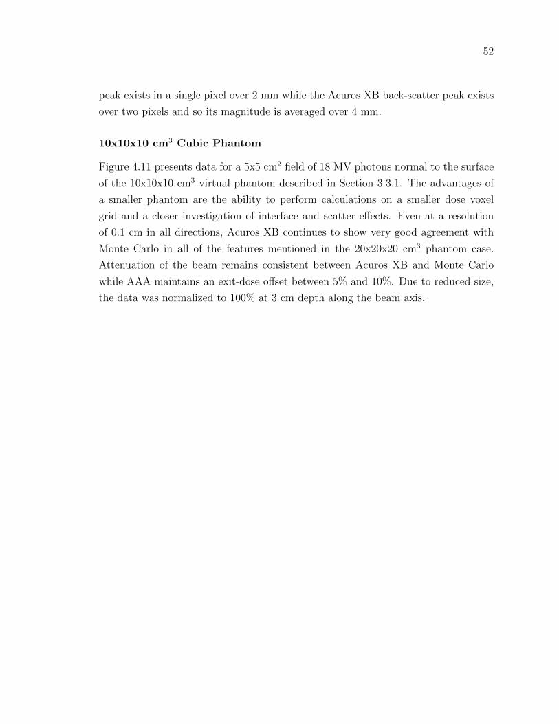
52

peak exists in a single pixel over 2 mm while the Acuros XB back-scatter peak exists

over two pixels and so its magnitude is averaged over 4 mm.

10x10x10 cm3 Cubic Phantom

Figure 4.11 presents data for a 5x5 cm2 field of 18 MV photons normal to the surface

of the 10x10x10 cm3 virtual phantom described in Section 3.3.1. The advantages of

a smaller phantom are the ability to perform calculations on a smaller dose voxel

grid and a closer investigation of interface and scatter effects. Even at a resolution

of 0.1 cm in all directions, Acuros XB continues to show very good agreement with

Monte Carlo in all of the features mentioned in the 20x20x20 cm3 phantom case.

Attenuation of the beam remains consistent between Acuros XB and Monte Carlo

while AAA maintains an exit-dose offset between 5% and 10%. Due to reduced size,

the data was normalized to 100% at 3 cm depth along the beam axis.

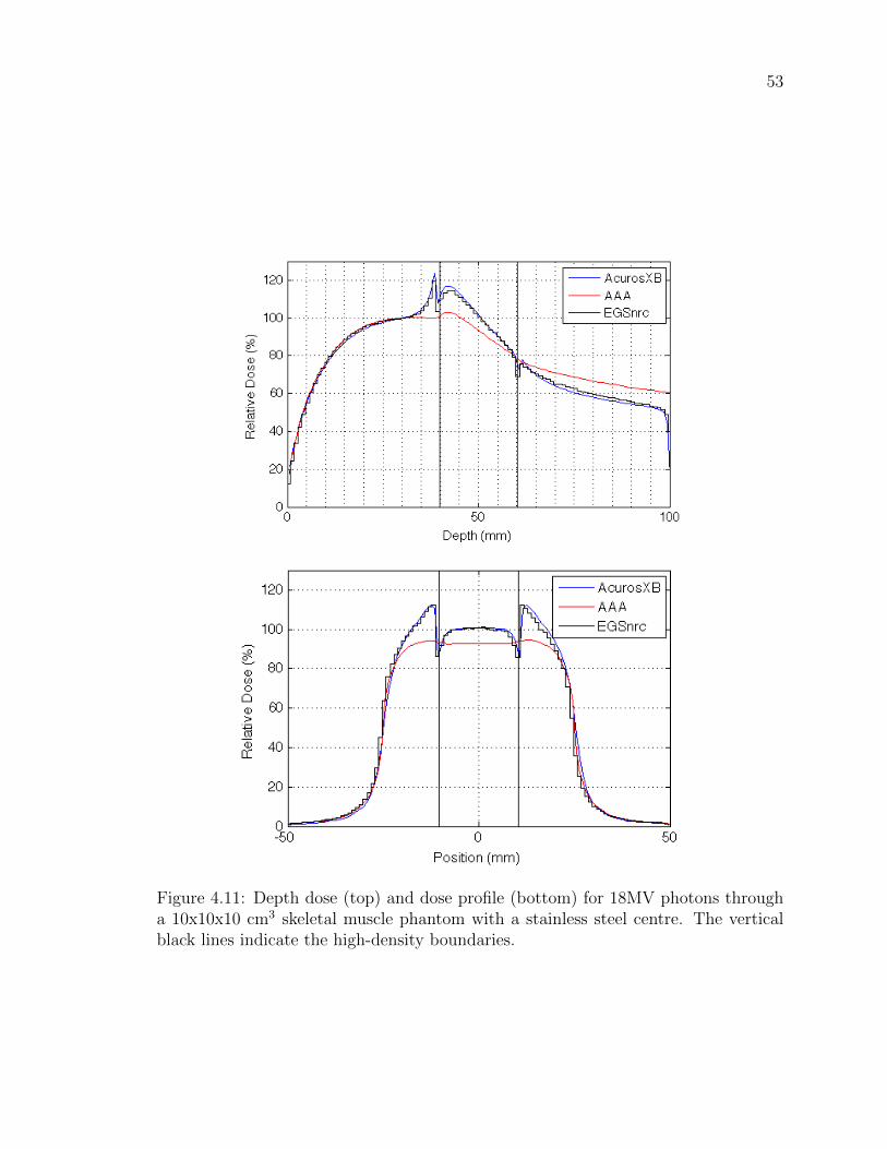
53

Figure 4.11: Depth dose (top) and dose profile (bottom) for 18MV photons througha 10x10x10 cm3 skeletal muscle phantom with a stainless steel centre. The verticalblack lines indicate the high-density boundaries.

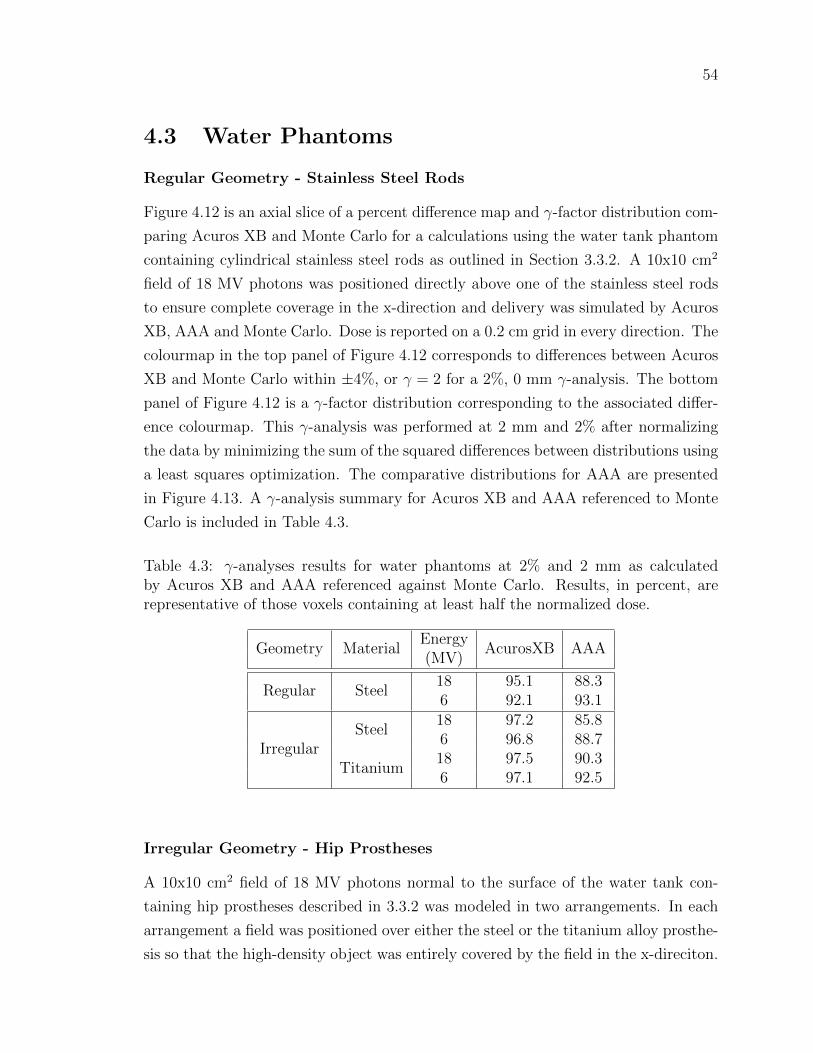
54

4.3 Water Phantoms

Regular Geometry - Stainless Steel Rods

Figure 4.12 is an axial slice of a percent difference map and γ-factor distribution com-

paring Acuros XB and Monte Carlo for a calculations using the water tank phantom

containing cylindrical stainless steel rods as outlined in Section 3.3.2. A 10x10 cm2

field of 18 MV photons was positioned directly above one of the stainless steel rods

to ensure complete coverage in the x-direction and delivery was simulated by Acuros

XB, AAA and Monte Carlo. Dose is reported on a 0.2 cm grid in every direction. The

colourmap in the top panel of Figure 4.12 corresponds to differences between Acuros

XB and Monte Carlo within ±4%, or γ = 2 for a 2%, 0 mm γ-analysis. The bottom

panel of Figure 4.12 is a γ-factor distribution corresponding to the associated differ-

ence colourmap. This γ-analysis was performed at 2 mm and 2% after normalizing

the data by minimizing the sum of the squared differences between distributions using

a least squares optimization. The comparative distributions for AAA are presented

in Figure 4.13. A γ-analysis summary for Acuros XB and AAA referenced to Monte

Carlo is included in Table 4.3.

Table 4.3: γ-analyses results for water phantoms at 2% and 2 mm as calculatedby Acuros XB and AAA referenced against Monte Carlo. Results, in percent, arerepresentative of those voxels containing at least half the normalized dose.

Geometry MaterialEnergy

AcurosXB AAA(MV)

Regular Steel18 95.1 88.36 92.1 93.1

IrregularSteel

18 97.2 85.86 96.8 88.7

Titanium18 97.5 90.36 97.1 92.5

Irregular Geometry - Hip Prostheses

A 10x10 cm2 field of 18 MV photons normal to the surface of the water tank con-

taining hip prostheses described in 3.3.2 was modeled in two arrangements. In each

arrangement a field was positioned over either the steel or the titanium alloy prosthe-

sis so that the high-density object was entirely covered by the field in the x-direciton.

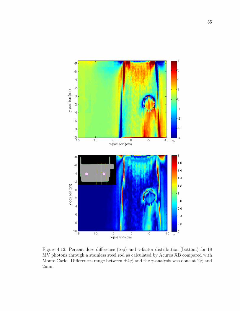
55

Figure 4.12: Percent dose difference (top) and γ-factor distribution (bottom) for 18MV photons through a stainless steel rod as calculated by Acuros XB compared withMonte Carlo. Differences range between ±4% and the γ-analysis was done at 2% and2mm.

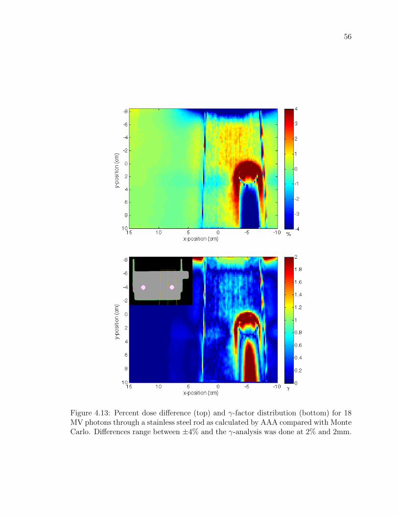
56

Figure 4.13: Percent dose difference (top) and γ-factor distribution (bottom) for 18MV photons through a stainless steel rod as calculated by AAA compared with MonteCarlo. Differences range between ±4% and the γ-analysis was done at 2% and 2mm.

57

Calculations were performed by Acuros XB, AAA and Monte Carlo on a 0.2 cm

dose grid in every direction. Dose distribution differences between Acuros XB and

Monte Carlo for both arrangements are displayed in the top panels of Figures 4.14

Figure 4.14: Percent dose difference (top) and γ-factor distribution (bottom) for 18MV photons through a steel alloy hip prosthesis as calculated by Acuros XB comparedwith Monte Carlo. Differences range between ±4% and the γ-analysis was done at2% and 2 mm.

58

and 4.15. Again, the differences displayed are between ±4%. The bottom panels

of Figures 4.14 and 4.15 are the corresponding γ-factor distributions, evaluated for

2% and 2 mm. Figure 4.16 shows comparative γ-analyses for AAA data referenced

Figure 4.15: Percent dose difference (top) and γ-factor distribution (bottom) for 18MV photons through a titanium alloy hip prosthesis as calculated by Acuros XBcompared with Monte Carlo. Differences range between ±4% and the γ-analysis wasdone at 2 mm and 2%.

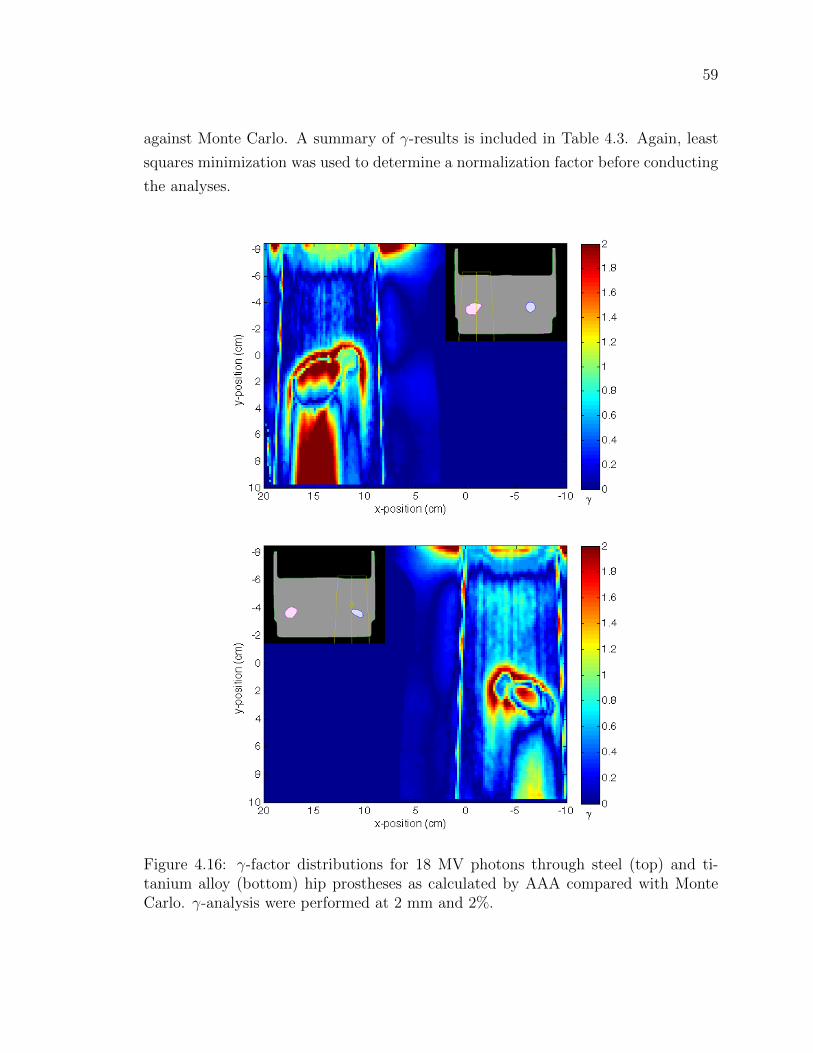
59

against Monte Carlo. A summary of γ-results is included in Table 4.3. Again, least

squares minimization was used to determine a normalization factor before conducting

the analyses.

Figure 4.16: γ-factor distributions for 18 MV photons through steel (top) and ti-tanium alloy (bottom) hip prostheses as calculated by AAA compared with MonteCarlo. γ-analysis were performed at 2 mm and 2%.

60

4.4 Patient Case

Figure 4.17 shows field arrangements for the first stage of a prostate treatment plan

for a patient who received radiation therapy at VIC in February 2011. The plan

was calculated using AAA and approved for delivery. As can be seen on the CT,

the patient has a unilateral left hip prosthesis which necessitated modification of the

Figure 4.17: Treatment plan field arrangement for a prostate patient with a unilateralhip prosthesis.

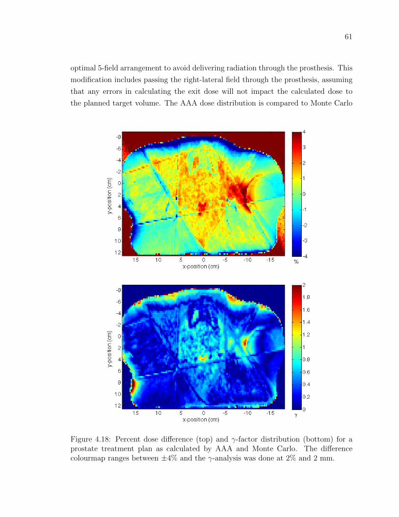
61

optimal 5-field arrangement to avoid delivering radiation through the prosthesis. This

modification includes passing the right-lateral field through the prosthesis, assuming

that any errors in calculating the exit dose will not impact the calculated dose to

the planned target volume. The AAA dose distribution is compared to Monte Carlo

Figure 4.18: Percent dose difference (top) and γ-factor distribution (bottom) for aprostate treatment plan as calculated by AAA and Monte Carlo. The differencecolourmap ranges between ±4% and the γ-analysis was done at 2% and 2 mm.

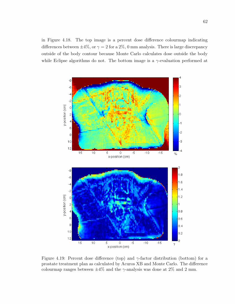
62

in Figure 4.18. The top image is a percent dose difference colourmap indicating

differences between±4%, or γ = 2 for a 2%, 0 mm analysis. There is large discrepancy

outside of the body contour because Monte Carlo calculates dose outside the body

while Eclipse algorithms do not. The bottom image is a γ-evaluation performed at

Figure 4.19: Percent dose difference (top) and γ-factor distribution (bottom) for aprostate treatment plan as calculated by Acuros XB and Monte Carlo. The differencecolourmap ranges between ±4% and the γ-analysis was done at 2% and 2 mm.

63

2% and 2 mm after normalizing the data by a factor determined by least squares

minimization. 97.0% of voxels containing at least 1% of the maximum dose were

within γ-tolerance.

For this research, the treatment plan was recalculated using Acuros XB and com-

pared with Monte Carlo. The resulting percent dose difference and γ-factor map

are shown in Figure 4.19. The evaluations were performed in the same manner as

indicated for the AAA, again subject to a normalization factor determined by least

squares. 98.7% of voxels containing at least 1% of the maximum dose were within

γ-tolerance. Even in this clinical case, where the presence of multiple fields is ex-

pected to minimize errors through averaging, Acuros XB still demonstrates improved

accuracy on the inside surface of the hip prosthesis.

4.5 Computation time

The introduction of an algorithm with a comparable degree of accuracy to Monte

Carlo has little advantage to radiotherapy planners unless it can be used at clinical

time scales. The times required to calculate a selection of dose distributions using

Monte Carlo, AAA and AcurosXB are displayed in Table 4.5. Monte Carlo calcula-

tions were performed on the 36 CPU cluster described in Section 3.1.1 while Acuros

XB and AAA calculations were done with dual quad-core CPUs and 24 GB of 1066

MHz RAM.

Table 4.4: Computation times for Monte Carlo, AAA and Acuros XBCalculation Field Size Resolution Energy Calculation Time

Volume (cm3) (cm2) (cm) (MV ) MC AAA AXB

10x10x10 5x5 0.118 29.6 hrs 8 sec 6.8 min6 13.9 hrs 8 sec 4.9 min

20x20x20 10x10 0.218 38.9 hrs 12 sec 3.0 min6 15.6 hrs 5 sec 2.2 min

64

Chapter 5

Discussion of Results

Results of the film measurements outlined in Section 3.2 were presented and discussed

in Section 4.1. The conclusion of this brief investigation is that the 30% forward-

scatter dose peak presented in Figure 3.2 is not expected in measurements or accurate

model calculations for 18 MV photons through a high-density inhomogeneity [11]. The

focus of Chapter 5, then, shall be an evaluation of the experimental dose distribution

data presented in Chapter 4 and the performance of Acuros XB in dealing with

increased photon and electron scatter due to high-density objects.

A quantitative comparison of 3-D dose distributions can be a somewhat arbitrary

exercise and there is no easy definition of a match as small differences in calculation

results are often impossible to measure dosimetrically. Tools such as γ-analyses can

be useful in providing a quantity that can be easily reported, but the significance of

that value can be easily undermined by biased evaluation conditions: when 90% of

a volume receives 0 Gy it is easy to report that your results have performed within

γ-tolerance with 90% success. In an attempt to avoid such volume effects, the γ-

analysis results tabulated in Chapter 4 include only those voxels containing at least

half the maximum dose for virtual phantom calculations and half the normalized

dose for water phantom calculations where the normalized dose was selected through

a least squares minimization of the total difference between the data to be evaluated

and Monte Carlo. In a patient case, any dose is significant when delivered to healthy

tissue, so a 1% dose threshold was used to remove dose to air from the patient case

analysis.

Substantial efforts were taken to eliminate systematic differences between data

generated by Acuros XB and data generated by Monte Carlo. Material data and

cross sections in Monte Carlo were made to match those used in Eclipse and both

65

systems were configured to model the output of the same clinical linear accelerator

used for treatment at VIC. Despite the best attempts, however, there were some

elements of the input data that could not be made uniform between systems.

As discussed in Section 2.3.2, there can be up to a whole pixel offset in the same

image or dose distribution depending on the spatial interpretation of a pixel’s position

by the software generating or displaying the data. Release notes from Varian Medical

Systems regarding Eclipse algorithms have indicated that the position of a contour

boundary may be incorrect by up to one calculation voxel as interpreted by Acuros

XB. This sort of position offset may result in the corresponding offset of a back- or

lateral-scatter peak, as is evident in the right lateral-peaks in Figures 4.2–4.6 and

4.11, and the left-lateral peaks in Figures 4.7 and 4.9.

The use of an adaptive mesh grid for calculations means that dose reported by

Acuros XB has been interpolated onto a fixed grid which introduces averaging effects

to the solution, and discretization of angle and energy introduces systematic error into

the Acuros XB solution, although Eclipse documentation limits this error at 0.1%. In

a Monte Carlo calculation, the implication of simulating a finite number of particles

is a degree of uncertainty in the final result. The Monte Carlo calculations performed

here have, on average, 1–2% standard deviation in the final dose distributions, pro-

ducing a noisy signal compared to Acuros XB and AAA and further reducing the

significance of a voxel by voxel difference. These, and the limitations listed above

should all be considered throughout the evaluation of Acuros XB that follows.

5.1 Virtual Phantoms

The purpose of investigating a geometrically ideal, virtual phantom is to reduce po-

tential sources of variation and determine if an algorithm is capable of treating the

simplest scenario accurately. Failure at this level might preclude any further inves-

tigation. A preliminary, qualitative overview of the dose distribution data presented

in Figures 4.2 and 4.11 of the 20x20x20 cm3 and 10x10x10 cm3 virtual phantoms,

respectively, indicates that Acuros XB is capable of accurately modeling the increase

in electron scatter due to the presence of a high-density object. Acuros XB data

shows appropriate dose peaks at the entrance and lateral surfaces of the high-density

region as expected, and as predicted by Monte Carlo data.

Continuing qualitatively, consider the oblique field delivery presented in Figure

4.6. This calculation was performed to determine the effect, if any, of non-normal

66

photon incidence on the accuracy of scatter modeling by Acuros XB. From these

depth dose and dose profile samples it appears that interface orientation has very

little, if any impact on the algorithm’s accuracy. The same conclusions can be drawn

for the variant cases presented in Figures 4.4–4.9 which include 6 MV photons and

titanium alloy inhomogeneities.

The quantitative analysis summarized in Table 4.1 presents an interesting picture

of algorithm performance. The γ-analyses parameters used, 2% and 2 mm, were

chosen to be representative of expected uncertainty bounds: 2 mm is the dimension

of a single dose voxel while 2% represents a reasonable bound on Monte Carlo data

variance. In comparison with Monte Carlo, Acuros XB is within γ-tolerance for

greater than 96.5% of voxels considered in all cases. In contrast, the highest γ-

success percentage for AAA is 92.9% while its worst agreement, in the case of the

obliquely delivered field, is 60.9%. Overall, these results suggest Acuros XB to be

better equipped to deal with high-density volumes than AAA.

5.2 Water Phantoms

Generally, agreement between Acuros XB and Monte Carlo is similar for the water

phantom and the virtual phantom calculations. A summary of γ-analysis results is

presented in Table 4.3. Acuros XB γ-tolerances range from 92% of voxels considered

in the case of a 6 MV field through a cylindrical stainless steel rod, to 97.5% of voxels

considered for an 18 MV field through a titanium alloy prosthesis. AAA γ-analysis

results for the same set of calculations range from 85.8% in the case of an 18 MV

field through a steel alloy prosthesis to a maximum of 93.13% in the case of a 6 MV

field through a cylindrical stainless steel rod.

The increase of geometric complexity in the water phantom cases, as well as

the reduction of contour quality with the introduction of image noise suggests an

increased degree of variance between calculation results. The uncertainty in boundary

definition combined with variations in boundary interpretation may very well account

for a majority of discrepancies between Acuros XB and Monte Carlo. Referring to

the difference maps in Figures 4.12, 4.14 and 4.15, regions of disagreement tend to

exist primarily at the phantom surface and at high-density interfaces, all of which are

subject to the listed sources of variation.

67

5.3 Patient Case

Because a clinical treatment plan often contains multiple fields with unique shapes

delivered from various angles, differences in dose distributions between algorithms are

expected to be somewhat washed or averaged out. Attempting to identify a modeling

flaw as the source of a dose discrepancy is better suited to the phantom cases discussed

in preceding sections. The purpose of this clinical case is to illustrate the impact of

modeling shortfalls and strengths in a clinical environment.

Figure 4.18 shows the discrepancies between AAA and Monte Carlo for the treat-

ment fields shown in Figure 4.17. A γ-analysis of these distributions shows a 97.0%

agreement at 2% and 2 mm for those voxels containing at least 1% of the normalized

dose. This is an excellent success rate, however, from an axial slice of the dose-

difference, AAA clearly demonstrates an underestimate of dose on the inside surface

of the prosthesis, represented in the dose difference plot by a region of dark red and a

smaller region of red in the γ-factor plot. This is a region of the metal structure that

likely has contact with bone, and depending on the severity of that underestimate,

this could lead to a radiation induced break or a secondary cancer.

The same difference map for Acuros XB is displayed in Figure 4.19 and there

are no comparable hot or cold spots. The γ-analysis results for the Acuros XB data

show 98.7% of voxels containing at least 1% of the normalized dose to be within

tolerance. This is an improvement over AAA, even if it is a quantitatively slight one.

In terms of target volume coverage and critical volume sparing there is little difference

between Acuros XB and AAA, but the absence of localized over- or under-dosage as

represented by Acuros XB is a significant result for clinical work and an advantageous

improvement for dosimetrists and oncologist planning around hip prostheses.

68

5.4 Summary

Overall, the preceding analyses have shown Acuros XB to be in better agreement with

Monte Carlo than AAA for dose calculations involving high-density volumes. The

magnitudes and extents of back- and lateral-scatter peaks are similar for Acuros XB

and Monte Carlo, and γ-analysis results are better for Acuros XB than for AAA when

evaluated against Monte Carlo. In addition, previously published data suggesting the

existence of a 30% forward-scatter peak has been discredited by film measurement.

In Chapter 6, the final chapter of this thesis, the implications of these findings and

remaining considerations are discussed.

69

Chapter 6

Conclusions & Considerations

The purpose of this research is to determine whether the solutions presented by

Acuros XB hold true to the physical principles governing radiation transport after

the introduction a high-density inhomogeneity to the calculation volume. It is not

within the scope of this project to conclude that Acuros XB is or is not acceptable

for clinical use. The clinical commissioning and implementation of a novel algorithm

is left to the medical physicists guiding and evaluating this work.

The first successful result for Acuros XB was the qualitative match with film mea-

surements taken for 18 MV photons through a high-density slab geometry, featuring

a sharp backscatter peak on the proximal surface of the inhomogeneity and the ab-

sence of a forward scatter peak on its distal surface. Considering the position and

calibration uncertainties associated with the measured data but not accounted for in

the plotted error bars and the boundary definition uncertainty associated with calcu-

lated data, this might also be considered a quantitative success, as the discrepancies

between Acuros XB and measured data are between 0.7 and 3.3% away from the

high-density boundaries. The agreement between measured and Monte Carlo data is

even better, ranging between 0.03 to 1.6% away from the boundaries.

The next positive result was in the modeling of lateral scatter from the high-

density region demonstrated by the virtual phantom calculations. This effect was

not accurately reflected in AAA data and may prove too difficult to be handled by a

convolution-superposition algorithm. Acuros XB was able to consistently match its

lateral peaks and other perturbation features with those modeled by Monte Carlo,

regardless of beam angle, energy or complexity of the high-density contour.

γ-analysis pass statistics, which were in excess of 95% in all but one case when

performed at 2% and 2 mm constraints, strongly suggest an algorithm capable of

70

reflecting the physics of radiation transport as accurately as Monte Carlo. The dif-

ferences that do exist between Acuros XB and Monte Carlo, for the most part, would

be nearly impossible to measure dosimetrically. In fact, when these tiny effects are

added up in a typical treatment plan they nearly vanish, as demonstrated by the

98.7% γ-analysis pass statistic for the prostate plan examined. Not only does Acuros

XB perform with accuracy comparable to Monte Carlo, it does so at time scales en-

tirely appropriate for a clinical planning, making it eligible for clinical consideration.

The implementation of a calculation algorithm such as Acuros XB would not

change the way dosimetrists and oncologist plan treatments for patients with hip

prostheses, rather, it would increase the confidence with which they do so. Regard-

less of the accuracy with which one can predict the dose distribution in and around

a high-density object, the resulting dose shadow means that treating through a pros-

thesis is an ineffective means of dose delivery and will increase the dose required to

treat the target volume to prescription, as well as increase the dose delivered to tissue

adjacent to the prosthesis. If this were not enough, variability in day-to-day position-

ing of the patient on the treatment couch adds the risk of misaligning the prosthesis

and overdosing everything beyond it. Instead, the implementation of an algorithm

like Acuros XB would allow for better informed treatment planning, eliminating the

uncertainty currently associated with planning around high-density regions.

Accuracy in modeling photon and electron scatter due to a high-density object

is only part of the challenge involved in planning for such cases. Considering Figure

1.2 and the discussion of artifacts in Section 2.3.1, there remains a loss of density

information due to the high-density region. CT shadows are often contoured and

assigned appropriate tissue-equivalent properties, but streaks are difficult to negate

and a contoured CT is still an approximation of reality. Techniques to correct high-

density artifacts, such as CT post-processing and multimodal imaging, are still in

development stage, and until they have been sufficiently validated for wide spread use,

a degree of approximation will remain in pelvic treatment planning around prostheses.

71

Overall, Acuros XB has been shown to perform as well as Monte Carlo for mod-

eling a dose distribution subject to increased photon and electron scatter due to the

presence of a high-density object. Until now, there has not been a clinically ap-

propriate algorithm available for such calculations. AAA, while acceptable for most

radiotherapy planning cases, has shown deficiencies in its ability to accurately re-

flect the full extent of the dose perturbations that result from increased photon and

electron scatter within a high-density volume. Once properly approved and commis-

sioned for clinical use, Acuros XB will be an important tool for planners dealing with

high-density implants.

72

Appendix A

Material Information

Table A.1: Material compositions for EGSnrc and Acuros

XB.

Material ElementWeight Fraction

EGSnrc AcurosXB

Air

C 0.000124

N 0.7552 0.755268

O 0.2318 0.231781

Ar 0.01283 0.012827

Lung

H 0.1030 0.101278

C 0.105 0.102310

N 0.031 0.028650

O 0.749 0.757072

Na 0.002 0.00184

Mg - 0.00073

P 0.002 0.0008

S 0.003 0.00225

Cl 0.003 0.00266

K 0.002 0.001940

Fe - 0.00037

Zn - 0.00001

73

Table A.1: (continued)


EGSnrc AcurosXB

Skeletal Muscle

H 0.100637

C 0.10783

N 0.02768

O 0.754773

Na 0.00075

Mg 0.00019

P 0.0018

S 0.00241

Cl 0.00079

K 0.00302

Ca 0.00003

Fe 0.00004

Zn 0.00005

Light Bone

H 0.085 0.096

C 0.404 0.099

N 0.028 0.022

O 0.367 0.744

Na 0.001 0.005

Mg 0.001 -

P 0.034 0.022

S 0.002 0.009

Cl 0.002 0.003

K 0.001 -

Ca 0.074 -

Fe 0.001 -

74

Table A.1: (continued)


EGSnrc AcurosXB

Bone

H 0.047234

C 0.14433

N 0.04199

O 0.446096

Mg 0.0022

P 0.10497

S 0.00315

Ca 0.20993

Zn 0.0001

Titanium Alloy

Ti 0.9

Al 0.06

V 0.04

Stainless Steel

C 0.0008

Si 0.01

P 0.00045

Cr 0.19

Mn 0.02

Fe 0.68375

Ni 0.095

75

Bibliography

[1] C. C. S. S. C. on Cancer Statistics, “Canadian cancer statistics 2011,” Totonto,

ON, 2011.

[2] M. Joiner and A. van der Kogel, eds., Basic Clinical Radiobiology. London:

Hodder Arnold, 4th ed., 2009.

[3] O. N. Vassiliev, T. A. Wareing, J. McGhee, G. Failla, M. R. Salehpour, and

F. Mourtada, “Validation of a new grid-based Boltzmann equation solver for

dose calculation in radiotherapy with photon beams,” Phys Med Biol, vol. 55,

pp. 581–98, Feb 2010.

[4] A. Clark, “The effect of the Roentgen Rays in a case of chronic carcinoma of the

breast,” British Medical Journal, vol. 1, no. 2110, p. 1398, 1901.

[5] F. M. Khan, The Physics of Radiation Therapy. Philadelphia, PA: Lippincott

Williams & Wilkins, 3rd ed., 2003.

[6] D. Thwaites and J. Tuohy, “Back to the future: the history and development of

the clinical linear accelerator,” Phys Med Biol, vol. 51, p. R343, 2006.

[7] W. Meredith, “40 years of development in radiotherapy,” Phys Med Biol, vol. 29,

p. 115, 1984.

[8] H. E. Johns and J. R. Cunningham, The Physics of Radiology. Springfield,

Illinois: Thomas, 4th ed., 1983.

[9] P. Litt, “Photon Finish: The Race to Build the Bomb,” Jun 2002.

[10] F. H. Attix, Introduction to Radiological Physics and Radiation Dosimetry. Wein-

heim, Germany: Wiley-VCH Verlag GmbH & Co., 2004.

76

[11] C. Reft, R. Alecu, I. Das, B. Gerbi, P. Keall, and E. Lief, “Dosimetric consider-

ations for patients with HIP prostheses undergoing pelvic irradiation. Report of

the AAPM Radiation Therapy Committee Task Group 63 prostheses undergo-

ing pelvic irradiation. Report of the AAPM Radiation Therapy Committee Task

Group 63,” Med. Phys., vol. 30, pp. 1162–1182, Jan 2003.

[12] K. A. Gifford, J. L. Horton, T. A. Wareing, G. Failla, and F. Mourtada, “Com-

parison of a finite-element multigroup discrete-ordinates code with Monte Carlo

for radiotherapy calculations,” Phys Med Biol, vol. 51, pp. 2253–2265, Apr 2006.

[13] K. Bush, I. M. Gagne, S. Zavgorodni, W. Ansbacher, and W. Beckham, “Dosi-

metric validation of Acuros R© XB with Monte Carlo methods for photon dose

calculations,” Med. Phys., vol. 38, no. 4, p. 2208, 2011.

[14] T. Han, J. K. Mikell, M. Salehpour, and F. Mourtada, “Dosimetric comparison

of Acuros XB deterministic radiation transport method with Monte Carlo and

model-based convolution methods in heterogeneous media,” Med. Phys., vol. 38,

p. 2651, Jan 2011.

[15] I. Gagne and S. Zavgorodni, “Evaluation of the analytical anisotropic algorithm

(AAA) in an extreme water-lung interface phantom using Monte Carlo dose

calculations,” Journal of Applied Clinical Medical Physics, vol. 8, no. 1, 2006.

[16] C. M. Bragg and J. Conway, “Dosimetric verification of the anisotropic analyt-

ical algorithm for radiotherapy treatment planning,” Radiother Oncol, vol. 81,

pp. 315–23, Dec 2006.

[17] I. J. Das and F. M. Kahn, “Backscatter dose perturbation at high atomic number

interfaces in megavoltage photon beams,” Med. Phys., vol. 16, pp. 367–75, Jan

1989.

[18] R. D. Evans, The Atomic Nucleus. New York, New York: McGraw-Hill, 1955.

[19] M. Woo and J. Cunningham, “The validity of the density scaling method in

primary electron transport for photon and electron beams,” Med. Phys., vol. 17,

pp. 187–194, 1990.

[20] W. Ulmer, J. Pyyry, and W. Kaissl, “A 3D photon superposition/convolution

algorithm and its foundation on results of Monte Carlo calculations,” Phys Med

Biol, vol. 50, pp. 1767–90, Apr 2005.

77

[21] G. M. Kremer, An Introduction to the Boltzmann Equation and Transport Pro-

cesses in Gases. Berlin, Germany: Springer-Verlag Berlin Heidelberg, 2010.

[22] I. Kawrakow and A. Bielajew, “On the representation of electron multiple elastic-

scattering distributions for Monte Carlo calculations,” Nucl. Instrum. Methods

B, vol. 134, no. 3-4, pp. 325–336, 1998.

[23] R. Koch and R. Becker, “Evaluation of quadrature schemes for the discrete

ordinates method,” J. Quant. Spectros. Radiat. Transfer, Jan 2004.

[24] J. T. Bushberg, J. A. Seibert, E. M. Leidholdt, and J. M. Boone, The Essential

Physics of Medical Imaging. Philadelphia, PA: Lippincott Williams & Wilkins,

2nd ed., 2002.

[25] J. Wei, G. Sandison, W. Hsi, M. Ringor, and X. Lu, “Dosimetric impact of a CT

metal artefact suppression algorithm for proton, electron and photon therapies,”

Phys Med Biol, Jan 2006.

[26] M. Aubin, O. Morin, J. Chen, and A. Gillis, “The use of megavoltage cone-beam

CT to complement CT for target definition in pelvic radiotherapy in the presence

of hip replacement,” British Journal of Radiology, Jan 2006.

[27] A. Niroomand-Rad, C. Blackwell, B. Coursey, K. Gall, J. Galvin, W. McLaugh-

lin, A. Meigooni, R. Nath, J. Rodgers, and C. Soares, “Radiochromic film dosime-

try: recommendations of AAPM radiation therapy committee task group 55,”

Med. Phys., vol. 25, pp. 2093–2115, 1998.

[28] I. Kawrakow, D. Rogers, F. Tessier, and B. Walters, “The EGSnrc code system:

Monte Carlo simulation of electron and photon transport,” Tech. Rep. PIRS-701,

National Research Council of Canada, Ottawa, Canada, 2010.

[29] B. Walters, I. Kawrakow, and D. Rogers, “DOSXYZnrc users manual,” Tech.

Rep. PIRS-794revB, Ottawa, Canada, 2009.

[30] D. Rogers, B. Walters, and I. Kawrakow, “BEAMnrc users manual,” Tech.

Rep. PIRS-0509(A)revL, National Research Council of Canada, Ottawa, Canada,

2009.

78

[31] G. Cranmer-Sargison, W. Beckham, and I. Popescu, “Modelling an extreme

water–lung interface using a single pencil beam algorithm and the Monte Carlo

method,” Phys Med Biol, vol. 49, p. 1557, 2004.

[32] D. A. Low, W. B. Harms, S. Mutic, and J. A. Purdy, “A technique for the

quantitative evaluation of dose distributions,” Med. Phys., vol. 25, pp. 656–61,

May 1998.

evaluation of a deterministic boltzmann solver for radiation therapy

Documents