NASA/TM–2003-212813

Evaluation of Genetic Algorithm ConceptsUsing Model ProblemsPart II: Multi-Objective Optimization

Terry L. Holst and Thomas H. Pulliam

December 2003

https://ntrs.nasa.gov/search.jsp?R=20040031786 2018-08-19T08:31:37+00:00Z

Since its founding, NASA has been dedicated to theadvancement of aeronautics and space science. TheNASA Scientific and Technical Information (STI)Program Office plays a key part in helping NASAmaintain this important role.

The NASA STI Program Office is operated byLangley Research Center, the Lead Center forNASA’s scientific and technical information. TheNASA STI Program Office provides access to theNASA STI Database, the largest collection ofaeronautical and space science STI in the world.The Program Office is also NASA’s institutionalmechanism for disseminating the results of itsresearch and development activities. These resultsare published by NASA in the NASA STI ReportSeries, which includes the following report types:

• TECHNICAL PUBLICATION. Reports ofcompleted research or a major significant phaseof research that present the results of NASAprograms and include extensive data or theoreti-cal analysis. Includes compilations of significantscientific and technical data and informationdeemed to be of continuing reference value.NASA’s counterpart of peer-reviewed formalprofessional papers but has less stringentlimitations on manuscript length and extentof graphic presentations.

• TECHNICAL MEMORANDUM. Scientific andtechnical findings that are preliminary or ofspecialized interest, e.g., quick release reports,working papers, and bibliographies that containminimal annotation. Does not contain extensiveanalysis.

• CONTRACTOR REPORT. Scientific andtechnical findings by NASA-sponsoredcontractors and grantees.

The NASA STI Program Office . . . in Profile

• CONFERENCE PUBLICATION. Collectedpapers from scientific and technical confer-ences, symposia, seminars, or other meetingssponsored or cosponsored by NASA.

• SPECIAL PUBLICATION. Scientific, technical,or historical information from NASA programs,projects, and missions, often concerned withsubjects having substantial public interest.

• TECHNICAL TRANSLATION. English-language translations of foreign scientific andtechnical material pertinent to NASA’s mission.

Specialized services that complement the STIProgram Office’s diverse offerings include creatingcustom thesauri, building customized databases,organizing and publishing research results . . . evenproviding videos.

For more information about the NASA STIProgram Office, see the following:

• Access the NASA STI Program Home Page athttp://www.sti.nasa.gov

• E-mail your question via the Internet tohelp@sti.nasa.gov

• Fax your question to the NASA Access HelpDesk at (301) 621-0134

• Telephone the NASA Access Help Desk at(301) 621-0390

• Write to:NASA Access Help DeskNASA Center for AeroSpace Information7121 Standard DriveHanover, MD 21076-1320

NASA/TM–2003-212813

Evaluation of Genetic Algorithm ConceptsUsing Model ProblemsPart I: Multi-Objective Optimization

Terry L. HolstAmes Research Center, Moffett Field, California

Thomas H. PulliamAmes Research Center, Moffett Field, California

December 2003

National Aeronautics andSpace Administration

Ames Research CenterMoffett Field, California 94035-1000

Available from:

NASA Center for AeroSpace Information National Technical Information Service7121 Standard Drive 5285 Port Royal RoadHanover, MD 21076-1320 Springfield, VA 22161(301) 621-0390 (703) 487-4650

EVALUATION OF GENETIC ALGORITHM CONCEPTS USING MODEL PROBLEMS

PART II: MULTI-OBJECTIVE OPTIMIZATION

Terry L. Holst and Thomas H. Pulliam NASA Ames Research Center

Moffett Field, CA 94035

Abstract

A genetic algorithm approach suitable for solving multi-objective optimization problems is described and evaluated using a series of simple model problems. Several new features including a binning selection algorithm and a gene-space transformation procedure are included. The genetic algorithm is suitable for finding pareto optimal solutions in search spaces that are defined by any number of genes and that contain any number of local extrema. Results indicate that the genetic algorithm optimization approach is flexible in application and extremely reliable, providing optimal results for all optimization problems attempted. The binning algorithm generally provides pareto front quality enhancements and moderate convergence efficiency improvements for most of the model problems. The gene-space transformation procedure provides a large convergence efficiency enhancement for problems with non-convoluted pareto fronts and a degradation in efficiency for problems with convoluted pareto fronts. The most difficult problems—multi-mode search spaces with a large number of genes and convoluted pareto fronts—require a large number of function evaluations for GA convergence, but always converge.

Nomenclature F set of scalar objective functions F∗ optimal set of F values f scalar objective function f ∗ maximum value of f Gn GA generation nth

IR integer ranking array ISELECT user-specified integer parameter controlling which selection algorithm is used ITRAN user-specified integer parameter controlling the gene-space transformation option NSEED user-specified parameter that controls how many solutions with different initializing

random number generator seeds are averaged together to construct a single convergence history curve

NC fixed number of chromosomes in each GA generation NCO number of constraints NG number of genes in each chromosome NM number of modes (hills or peaks) associated with the MP1 and MP2 model problems NO number of scalar objective functions P user-specified vector with four elements that controls which modification operators are

used in going from G to Gn n+1 p1 user-specified parameter controlling the probability that a specific gene will be modified

using the perturbation mutation operator (0 ≤ p1 ≤ 1) p2 user-specified parameter controlling the probability that a specific gene will be modified

using the global mutation operator (0 ≤ p2 ≤ 1) R basis vector matrix with elements ri ,j

R(0,1) random number generator that returns a random value between 0 and 1

1

U unitary transformation matrix with elements u i, j

x i,jn i th gene from the chromosome from the n GA generation j th th

X jn chromosome from the GA generation j th nth

xmaxi user-specified maximum limit on the i th gene

xmini user-specified minimum limit on the i th gene

β user-specified parameter controlling the size of the perturbation mutations (0 ≤ β ≤ 1) subscripts

gene or decision variable index ij chromosome index k objective function index m mode index (associated with MP1 and MP2) superscripts

GA generation or population index nt temporary chromosome and gene values obtained after selection but before operator

modification

Background Numerical methods for optimizing the performance of engineering problems have been studied for many years. Perhaps the most widely used general approach involves the computation of sensitivity gradients. These methods—called gradient methods—have been utilized to produce optimal engineering performance in a wide variety of different forms. The reliability and success of gradient methods generally requires a smooth design space and the existence of only a single global extremum or an initial guess close enough to the global extremum that will ensure proper convergence. In contrast to gradient-based methods, design space search methods such as genetic algorithms (GA)—also referred to as evolutionary algorithms (EA)—offer an alternative approach with several attractive features. The basic idea associated with the GA approach is to search for optimal solutions using an analogy to the theory of evolution. The problem to be optimized is parameterized into a set of decision variables or genes. Each set of genes that fully defines one design is called an individual or a chromosome. A set of chromosomes is called a population or a generation. Each complete design or chromosome is evaluated using a “biological-like” fitness function that determines survivability of that particular chromosome. For example, in aerospace applications, the genes may be a series of geometric parameters associated with an aerospace vehicle that is to be optimized for payload delivered to orbit, aerodynamic performance or structural weight. The fitness function takes as input all the geometric parameters and returns a numerical value for the fitness—the size of the payload, the aerodynamic performance or the structural weight. During solution advance (or “evolution” using GA terminology) each chromosome is ranked according to its fitness vector—one fitness value for each objective. The higher-ranking chromosomes are selected to continue to the next generation while the lower-ranking chromosomes are not selected at all. The newly selected chromosomes in the next generation are manipulated using various operators (combination, crossover or mutation) to create the final set of chromosomes for the new generation. These chromosomes are then evaluated for fitness and the process continues—iterating from generation to generation—until a suitable level of convergence is obtained or until a specified number of generations has been completed. Constraints can easily be included in the GA optimization approach either by direct inclusion into the fitness function definition—a so-called penalty constraint—or, more commonly, by including one or more

2

constraints into the fitness function evaluation procedure. For example, if a design violates a constraint, its fitness is set to zero, i.e., it does not survive to the next generation. Because GA optimization is not a gradient-based optimization technique, it does not need sensitivity derivatives. It theoretically works well in non-smooth design spaces containing several or perhaps many local extrema. General GA details including descriptions of basic genetic algorithm concepts can be found in Goldberg,1 Davis,2 and Beasley, et al.3,4 Additional useful studies, which survey recent activities in the area of genetic algorithm or evolutionary algorithm research including the presentation of model problems useful for evaluating GA performance are given in Deb,5 Van Veldhuizen and Lamont6 and Jiménez, et al.7 A disadvantage of the GA approach is expense. In general, the number of function evaluations required for a GA optimization process to converge, exceeds the number of function evaluations required by a finite-difference-based gradient optimization (see the results presented in Obayashi and Tsukahara8 and Bock9). This situation is offset, to an extent, by the ease with which GAs can be implemented in parallel or distributed computing environments. Despite being relatively new, genetic algorithms have already been applied in many applications over a broad range of engineering fields. A brief survey of single discipline applications is presented in Holst and Pulliam,10 and will not be discussed further in this report. Other applications involving GA search methods have been made in the area of multi-objective or multi-discipline optimization, i.e., optimization problems in which two or more objectives are simultaneously optimized. These methods, referred to as MOGA (multi-objective genetic algorithm) methods, are especially attractive because they offer the ability to directly compute so-called “pareto optimal sets” in a single computation instead of the limited single design point traditionally provided by other methods. The pareto optimal set or pareto front, as it is common called, includes optimal solutions for each of the individual objectives, as well as a range of tradeoff solutions in between, which are themselves optimal solutions. Providing a range of solutions to a multi-objective optimization problem is a powerful approach because it allows the designer to see the effect of decision variable variation on the design space in the form of optimal tradeoffs. Thus, the designer can choose individual objective weighting factors after their full influence is quantitatively known. In recognition of the importance of the MOGA approach, many theoretical developments have been published in recent years. In particular, Van Veldhuizen and Lamont,6 and Zitzler, et al.11 present reasonably complete surveys of MOGA methodology with a special emphasis on how to compare GA performance from one algorithm variation to another. Other researchers, including Deb,5 Deb, et al.,12 Van Veldhuizen13 and Lohn, et al.,14 have developed and/or utilize a suite of test problems as a standard in evaluating MOGA convergence efficiency as well as the accuracy of the final pareto front. A key aspect of pareto front development is diversity. Does a particular MOGA produce good coverage over the entire pareto front or are some regions poorly resolved while other regions have high levels of undesirable clustering? This issue is studied in Laumanns, et al.15 and Deb, et al.16

Still other MOGA issues are associated with archive strategies. As the pareto front develops, many solutions are found that lie on the pareto front that cannot be retained within the fixed population size of many schemes. How to retain or archive this information for the benefit of the MOGA while maintaining reasonable bounds on the archive file has been studied in Knowles and Crone.17,18 One last example of MOGA research lies in the area of an interactive algorithm development. Parmee, et al.19 present a MOGA approach that allows changes to be made in GA operators as wells as in objective definitions as the MOGA advances from generation to generation. One area of MOGA research that is even more voluminous than the area of theoretical developments is that associated with GA multi-objective applications. Examples of multi-objective optimization applications include airfoil optimization by Marco, et al.,20 Naujoks, et al.,21 Quagliarella and Della Cioppa,22 Vicini and Quagliarella,23 Hämäläinen, et al.24 and Epstein and Peigin,25 missile aerodynamic shape optimization by

3

Anderson, et al.,26 wing optimization by Anderson and Gebert,27 Sasaki, et al.,28 Oyama,29 Obayashi, et al.,30 and Ng, et al.31

Additional MOGA examples in the area of turbomachinery optimization include rocket engine turbopump design by Oyama and Liou32 and compressor blade design by Benni33 and Oyama and Liou.34 In some of these examples the multiple objectives were obtained by considering two different aerodynamic design points. In others the multiple objectives involved different disciplines including aerodynamics, structures, controls and/or electromagnetics. One last area of MOGA research that bears mention is in the area of hybrid methods, the utilization of MOGA optimization in conjunction with another type of optimizer. This is an attractive area of research because MOGA methods are particularly good at finding a global extrema, but not particularly good in converging the optimal solution to tight levels of accuracy. Briefly, several examples where hybrid approaches have been utilized include Giotis, et al.35 and Tursi36 where a MOGA has been coupled to a neural network for aerodynamic shape optimization, and Vicini and Quagliarella37 and Brown and Smith38 where a MOGA has been coupled with a gradient optimizer. Various definitions and the multi-objective genetic algorithm used in the present study are described next. Details associated with each of the operators, including selection, passthrough, random average crossover, perturbation mutation and mutation are presented. MOGA convergence efficiency is then evaluated using several model problems from two general points of view—the effect of design space characteristics on GA convergence and the effect of GA control parameter specification on GA convergence.

Problem Statement: Single Objective Optimization A single-objective optimization problem can be stated as follows: Let f be a scalar function of N independent variables, x , defined on some domain

G

i Ω

f = f (X) = f (x1,L,xi ,L,xNG

) (1a)

In this notation X is the vector of design space decision variables. The maximum value of f , indicated by , is obtained by finding the values of Xf ∗ = X∗ such that†

f ∗ = max f = f (X∗) = f (x1

∗,L,xi∗,L,xNG

∗ ) (1b)

The above maximization operation is subject to N conditions or constraints indicated by CO

cn (X) ≤ 0 n = 1,2,L,NCO (1c)

The constraints placed on the decision variable vector X by Eqs. (1c) essentially serve to limit the design space within Ω for which the optimal solution is sought.

Problem Statement: Multi-Objective Optimization For optimization problems involving more than one objective, which are simultaneously optimized, the situation is more difficult. This is because each objective must play a role in determining the optimal solution. In the optimization process, conflicts might arise among the various objective functions, i.e., the

† For the purpose of simplifying the discussion of algorithmic details, maximization is generally assumed. The logic for minimization is a straightforward modification and will not be discussed.

4

optimal values of each individual objective, in general, will not occur for the same decision variable vector, . As a result, the “optimal solution” for a multi-objective optimization problem is typically a range or a set of solutions, which represent tradeoffs in objective space.

X

To determine when one solution is better than another for multi-objective problems the concept of dominance is utilized.1 A vector U = U(u1,L,ui ,L,uN ) is said to dominate another vector

V = V(v1,L,vi ,L,vN ) if and only if u for all and there exists at least one value of i such that u . A vector defined on some domain Ω that is not dominated by any other vector defined on Ω is said to be non-dominated on Ω .

i ≥ vi i i > vi

A multi-objective optimization problem can be stated as follows: Let be a set of N scalar objective functions, , each dependent upon the same decision variable vector,

F Ofk X , which is defined on some

design space Ω

F = F(f1(X),L,fk (X),L,fNO

(X)) (2a)

As above, the decision variable vector X consists of N independent components. The multi-objective optimization problem involves finding the set of

G

X = X∗ that produce non-dominated values for F = F∗ on . This set of values F is called the pareto optimal set or the pareto front. Ω ∗

For each F the constraints

cn (X) ≤ 0 n = 1,2,L,NCO (2b)

must be satisfied. Existence of these constraints serves to limit or reduce the size of Ω for which the optimal solution is sought.

Genetic Algorithm The genetic algorithm optimization procedure utilized to solve the multi-objective optimization problem, as described by Eqs. (2), is now presented. It is closed related to the GA optimization procedure presented in Holst and Pulliam,10 which was designed for single objective problems. As mentioned in the introduction, the general idea behind GA optimization is to discretely describe the design space using a number of decision variables, x . In GA parlance these parameters are called genes, and the i i subscript refers to the gene number. Each set of genes that leads to the complete specification of an individual design, i.e., each decision variable vector, X , is called a chromosome and is indicated by

(3) X j

n = X jn (x1,j

n ,L,xi ,jn ,L,xNG , j

n )

where the subscript, added to X , identifies the chromosome number. In addition, the subscript has been added to each gene, so as to indicate which chromosome each gene value is identified with. The n superscript had been added to indicate the GA generation number, which is iteratively advanced as the solution converges. Thus,X is the chromosome for the n generation that consists of N genes.

j j

jn j th th

G

For aerodynamic shape optimization problems, the design space genes are typically a series of geometric parameters, e.g., airfoil thickness and camber and/or wing sweep, twist and taper. For many GA applications genes are computationally represented using bit strings and the operators used to manipulate them are designed to accommodate bit string data. In the present approach, following the arguments of Oyama,39 Houck, et al.40 and Michalewicz,41 real-number encoding is used to represent all genes. The key reason for using real number encoding is that it has been shown to be more efficient in terms of CPU time relative to binary encoded GAs.41 In addition, real numbers are used for all genes in

5

the present implementation because many engineering applications involve decision variables that are best described using real numbers, e.g., the geometric parameters in aerodynamic shape optimization. Thus, using real number encoding eliminates the need for binary-to-real number conversions. Initialization Once the design space has been defined in terms of a set of real-number genes, the next step is to form an initial generation, G , represented by 0

(4)

G0 = (X1

0,L,X j0 ,L,XNC

0 )

where N is the total number of chromosomes. Each gene within each chromosome is assigned an initial numerical value using a process that randomly chooses numbers between fixed user-specified limits. For example, the

C

i th gene in an arbitrary chromosome is initialized using x i = R(0,1)(xmaxi

− xmini) + xmini

(5)

where and x are the upper and lower limits for the xmaxi minii th gene, respectively, and R is a

random number generator that delivers an arbitrary numerical value between 0.0 and 1.0. (0,1)

The random number generator used in the present study requires an integer input—a seed value. If the integer is positive, the next number in the current random number sequence is always returned. If the integer is negative, the random number sequence is reset. Utilization of the same negative seed value will always reset the random number generator to the same random sequence. Each new solution begins by resetting the random number generator using a single call to R with a negative seed value. All other calls to R during that solution use a positive seed value. Thus, a solution can be repeated by simply using the same initial seed value or rerun to determine statistical variation by using a different initial seed value.

(0,1)(0,1)

Fitness evaluation After a generation is established—either the initial generation or any of the succeeding generations in the evolutionary process—fitness values, F , are computed for each chromosome using a suitable function evaluation. This is analogous to the objective function evaluation in gradient methods and is represented using

jn

Fj

n = F(X jn ) (6)

For example, for a multi-discipline optimization (MDO) problems involving the simultaneous maximization of two separate and distinct objectives, f and , the fitness evaluation represented by Eq. (6) consists of the following

1 f2

f1

n = f1(X jn )

f2n = f2(X j

n )

where, for example, the first function f might be the aerodynamic drag of an aerospace vehicle (constrained to fly at fixed lift) and the second function f might be the structural mass of the same vehicle. Once all the genes in a specific chromosome have been specified, f can be evaluated using a suitable CFD solver to obtain the drag and f can be evaluated using a suitable structural analysis routine

1

2

1

2

6

to obtain the structural mass. In this case, of course, the optimization problem would be one of minimization. Ranking The purpose of the ranking operation is to determine a set of integer values for the ranking array, IR . One integer value is required for each chromosome. The ranking algorithm is quite different for multi-objective optimization problems relative to its single-objective counterpart. As such, both situations will be discussed in this section. The ranking array values—once determined—are then used in the GA selection process. Single Objective Optimization—The GA ranking algorithm for single objective optimization problems is quite simple. Whichever chromosome has the highest fitness is ranked number one ( IR = 1), whichever has the second highest fitness is ranked number two ( IR = 2 ), and so on. This ranking algorithm, more formally stated, is given by

(7)

ic = 1if (fj

n < fln ) ic = ic + 1 l = 1,L,NC

IRjn = ic

⎫

⎬ ⎪

⎭ ⎪

j = 1,L,NC

where and j l are special counters that range over all N chromosomes in the current population or generation level.

C

Multi-Objective Optimization—For multi-objective optimization problems the ranking procedure is more complex and utilizes the concept of dominance, which was defined previously. A chromosome with a fitness vector F that is not dominated by any other fitness vector within the design space is said to be a non-dominated chromosome. The optimal solution set F∗ or pareto front includes all solutions with fitness vectors that are non-dominated and that satisfy the constraints given by Eqs. (2b). The numerical approximation to the pareto front must involve a suitably complete set of discrete solutions so as to describe the optimal values of each individual objective—these are the pareto front endpoints—as well as the non-dominated tradeoff solutions in between the individual objective’s optimal values. The use of dominance for determining pareto fronts in multi-objective optimization problems can be clarified by considering a simple example involving two-objectives without constraints. When NO = 2 the optimization problem given by Eq. (2a) can be restated as

F = F f1 X( ),f2 X( )( ) (8)

The solution set for the problem defined in Eq. (8) contains all solutions with fitness vectors F = F(f1,f2) in the feasible domain that are non-dominated—or for numerical optimization, a suitably populated set of discrete solutions with fitness vectors that are non-dominated. For a design point ( to be non-dominated, there can exist no points in the design space ( such that

f1*,f2*)f1,f2)

f1 ≥ f1 * and f2 > f2 *

orf1 > f1 * and f2 ≥ f2 *

This situation is presented schematically in Fig. 1 where the shaded region is the feasible region of the design space and the thick dark line contains all members of the pareto front. The square symbols

7

represent the maximum values of each of the individual objectives and also serve to define the pareto front endpoints.

FEASIBLE REGION

INFEASIBLE REGION

f1

f2

PARETO FRONT

max f2

max f1

Fig. 1 Schematic of a two-objective design space in which f and f are simultaneously maximized. The thick dark line is the pareto front.

1 2

With the concept of dominance in hand the actual ranking process can now be presented. There are a number of ranking procedures available for use in multi-objective optimization. The one used in the present study is called Goldberg ranking.1 After all of the fitness values have been determined, each chromosome is checked for dominance. Those chromosomes that are non-dominated are given a number one ranking ( IR = 1) and then set aside. The remaining chromosomes that are non-dominated are given a number two ranking ( IR = 2 ) and then set aside. This process continues until each chromosome has an integer value for the ranking array, IR . In general, with this approach, the number of different integer values contained within the ranking array will be small, at least small in comparison to

, as many chromosomes will be ranked near the top with a value of 1, 2 or 3. NC The above procedure, by itself, represents a legitimate algorithm for the ranking operation. However, there is a refinement that provides a considerable enhancement to GA convergence. Before describing this refinement, two additional concepts must be defined—the active file and the accumulation file. The active file is simply a specific name used for the current generation of chromosomes, that is

Gn = (X1

n ,L,X jn,L,XNC

n ) is the n generation active file for the GA iteration process. As the GA solution evolves, the active file is always fixed in size at N chromosomes. The first N elements in the active file—for the present implementation—always contain the chromosomes that posses the maximum fitness values for each of the N objectives.

th

C O

O The accumulation file is the list of all non-dominated chromosomes that have been found from all generations combined. As the GA solution evolves, the accumulation file typically grows in size with more chromosomes being added after each new generation. As new non-dominated chromosomes are added to the accumulation file, old chromosomes that lose their dominance must be deleted, thus ensuring that the accumulation file contains nothing but number-one ranked chromosomes. Because each chromosome stored in the n generation accumulation file is non-dominated, it serves to define the pareto front or, at least, the n generation approximation to the pareto front. The use of an accumulation file makes sense only when N .

th

th

O ≥ 2

8

The multi-objective ranking procedure described above utilizes only the chromosomes in the active file, i.e., each chromosome in the active file is ranked relative to the other chromosomes in the active file. But this philosophy potentially wastes a plethora of information because not every number-one ranked chromosome for multi-objective optimization problems can be retained from one generation to the next in the active file. This is where the refinement in the ranking routine enters in. Once each chromosome in the active file is ranked using the standard routine, an additional test is performed to see if any number-one ranked chromosomes in the active file are dominated by any of the chromosomes in the accumulation file. If this is the case, then the ranking number associated with the newly ranked chromosome in the active file is decremented by one. This ensures that the ranking routine produces number one rankings that are number one in a global sense. Selection After the ranking array is established, with or without the accumulation file option, the GA algorithm passes to the selection process to determine which chromosomes will continue on to the generation and which will not. In the present study three different selection operators will be studied: (1) a new and simple technique called greedy selection, (2) a traditional algorithm called tournament selection, and (3) a third algorithm based on a “binning” strategy called bin selection. In each case the selection process picks established chromosomes—either from the n generation active file, X , or from the accumulation file—and then presents them to the modification process, which will be described shortly.

(n + 1)st

thjn

Greedy selection—This selection algorithm is quite simple. It selects all of its chromosomes from the n generation active file, i.e., from . It is implemented using the following

th

X jn

l = 1

if (IRjn ≤ l ) then

Xlt = X j

n

l = l + 1endif

⎫

⎬ ⎪ ⎪

⎭ ⎪ ⎪

j = 1,NC

if ( l > NC ) stop

⎫

⎬

⎪ ⎪ ⎪

⎭

⎪ ⎪ ⎪

i t = 1,NC (9)

where each selected chromosome X is placed in a temporary holding array indicated by l

t

Gt = (X1

t ,L,Xit ,L,XNC

t )

Note how the highest ranked individuals in the n generation are selected multiple times, individuals with average ranking are selected a small number of times, and individuals with the lowest rankings are not selected at all. This biasing toward individuals with the highest rankings is a key element in any GA. The chromosomes represented by G are next used by succeeding modification operators to produce

th

t Gn +1. Tournament selection—The tournament selection algorithm is quite simple and is used widely—one variation or another—in many GA optimization applications. The present variation is implemented as follows. Using a random process, three chromosomes are chosen from the n generation active file, i.e., from . The ranking array values, I

th

X jn R , are then compared. The chromosome with the highest ranking

array value is retained, being placed in a temporary holding array, G . In case of ties the chromosome selected first is retained and placed into the temporary holding array. This process continues until N

t

C

9

chromosomes have been selected. The chromosomes represented by G are next used by succeeding modification operators to produce G .

t

n +1

Bin selection—The bin selection algorithm is different from greedy and tournament selection, as implemented here, in two general ways. First, the bin selection algorithm chooses its chromosomes from the accumulation file, not the active file. Second, the bin selection algorithm divides the distance along the pareto front into equal segments or “bins” using an arc-length computation and then selects an equal number of chromosomes from each bin using a random process. As with the other options, the selected chromosomes are placed in a temporary holding array, G . t

Since this particular bin selection algorithm requires the computation of arc-length along the pareto front, it inherently requires optimization problems with only two objectives, i.e., the pareto fronts must be curves in two dimensions. Another option, which works for a general number of objectives, is available, but has not been utilized in the present study. The present bin selection algorithm attempts to improve the selection process in two ways. The equal partition of the pareto front based on arc-length—not on population—forces increased emphasis for selection from underdeveloped regions of the pareto front and reduced emphasis for selection from overdeveloped regions. This keeps unwanted clustering from occurring and allows details from all portions of the pareto front to develop. Such a selection algorithm might be particularly useful for problems that have disjoint or discontinuous pareto fronts, which are often associated with design spaces that contain one or more local optima, whether the design space is smooth or not. Since the chromosomes that are selected all possess number one rankings, the chance that a superior set of chromosomes will be selected using this option is increased, i.e., the chance that the GA will converge more quickly is increased. This later characteristic, while likely, is not assured for all optimization problems. This is because some pareto fronts are most optimally approached using modification operators that require information from the non-optimal design space interior. Knowing which type of situation exists a priori is impossible for most realistic engineering design problems. Modification Operators P Vector—After the new chromosomes have been selected and placed in the temporary holding array,

, they must be modified using one of several modification operators to obtain the ( generation of chromosomes, . In the present implementation four modification operators are used—passthrough, random average crossover, perturbation mutation and mutation. How many chromosomes are modified with each operator is controlled by the

Gt n + 1)st

Gn +1

P vector, which consists of four parameters— , , , . Each element of the P vector controls one modification operator. The value of each P vector element ranges from 0 to 1.0, and, for consistency, the sum of all four elements must always equal one. A

pB pA pP pM

P vector equal to 0.1, 0.3, 0.3, 0.3, for example, will cause the first 10 percent of the chromosomes to be modified using the passthrough operator, the next 30 percent to be modified using random average crossover, the next 30 percent to be modified using perturbation mutation and the last 30 percent to be modified using mutation. That is, p , pB = 0.1 A = 0.3 , pP = 0.3 , and pM = 0.3 . The passthrough operator is always performed first. After passthrough is complete, the implementation order of the remaining operators is immaterial. Once all values of Gn +1 have been established, the algorithm proceeds to fitness evaluation, ranking and then onto succeeding generations until the optimization is sufficiently converged. Passthrough—The simplest operator used in the present GA is “passthrough.” As the name implies, a certain number of chromosomes with the highest individual fitness values are simply “passed through” to the next generation from G to G without modification. The number of chromosomes that are passed through to the next generation is controlled by the first parameter in the

t n +1

P vector, . The passthrough pB

10

operator is always performed on the first p chromosomes in G . Care must be taken when choosing

and N so that p . If this is done, the chromosomes with the highest individual fitness values will always be passed through to the next generation, thus guaranteeing that none of the individual maximum fitness values will ever drop during GA iteration.

BNCt

pB C BNC ≥ NO

Random average crossover—The next GA modification operator is called random average crossover and is implemented by first selecting two random chromosomes X and X from G . Next, the two selected chromosomes are combined on a gene-by-gene basis using the following formula:

j1t

j 2t t

x i,j

n+1 =12

(xi ,j 1t + xi ,j 2

t ) i = 1,2,L,NG (10)

where x corresponds to the i ,j

n +1 i th gene in the chromosome associated with G and

correspond to the

j th n +1 x i,j 1t and xi, j2

t

i th genes from the randomly chosen chromosomes X j1t and X j 2

t . The number of chromosomes modified using the random average crossover operator is determined by the parameter

—the second element in the pA P vector. Perturbation mutation—The next GA modification operator is called perturbation mutation and is implemented by first selecting a random chromosome X from G . Next, a probability test is performed

for each gene xjt t

i,jt in the selected chromosome involving a call to a random number generator R . If

the returned random number is less than p the gene is modified using (0,1)

1 (11) x i,j

n+1 = xi, jt + (xmax i

− xmini)[R(0,1) − 0.5]β

where β is a user-specified tolerance that controls the size of the perturbation mutation, and p is a user-specified control parameter that statistically controls the number of genes that are modified. For sensible results the values of

1

β and p must be between 0 and 1.0. 1 Because this operator can cause the value of a particular gene to exceed one of its constraints (x or

), checks are required to prevent this. The number of chromosomes modified using the perturbation mutation operator is determined by the parameter p —the third element in the

maxi

xmini

P P vector. Mutation—The last GA modification operator used in the present study is called mutation and is implemented similarly to the perturbation mutation operator. First, a random chromosome X j

t is chosen

from . Next, a probability test is performed for each gene xGti,jt in the selected chromosome involving a

call to a random number generator R . If the returned random number is less than p the gene is given a completely different value using

(0,1) 2

x (12) i,j

n+1 = (xmaxi− xmini

)R(0,1) + xmini

The parameter p is a user-specified control parameter that statistically controls the number of genes that are modified. For sensible results p must be between 0.0 and 1.0. The number of chromosomes modified using the mutation operator is determined by the parameter p —the fourth element in the P vector.

2

2

M

Gene-space transformation—An option for accelerating GA convergence for multi-objective optimization problems is described in this section. When modifying G to obtain Gt n+1 it is sometimes advantageous to first transform or reorient each chromosome using a gene-space transformation procedure. The

11

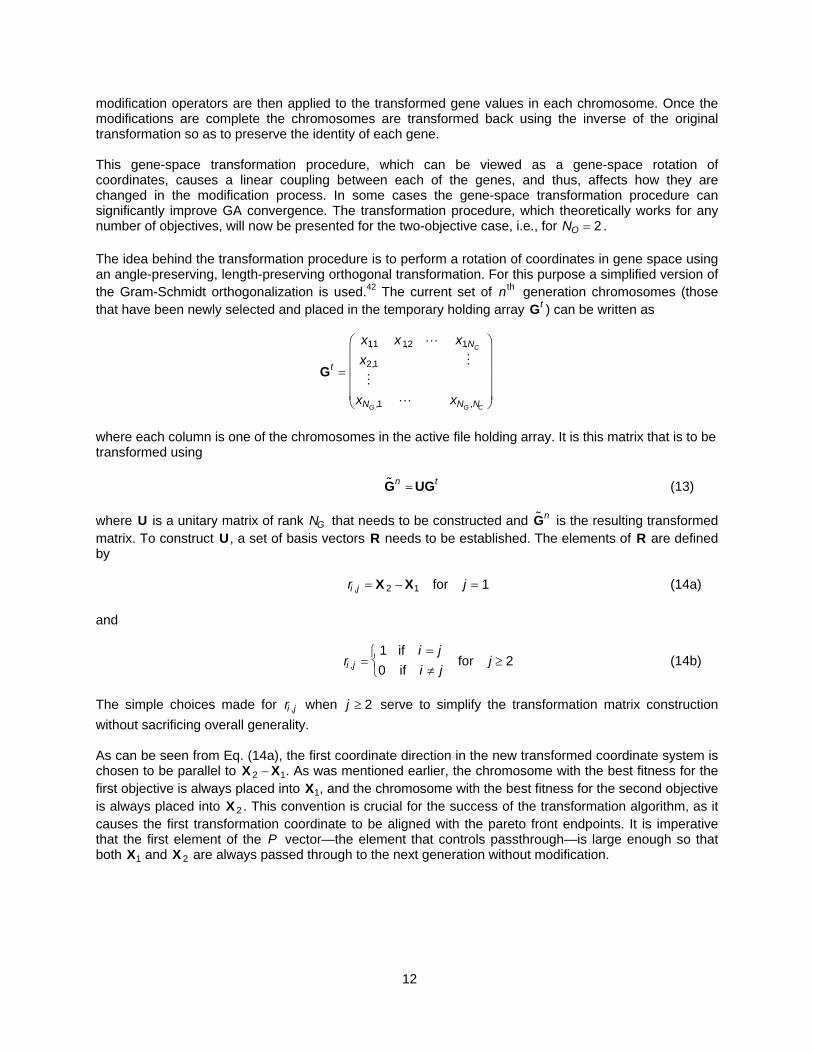
modification operators are then applied to the transformed gene values in each chromosome. Once the modifications are complete the chromosomes are transformed back using the inverse of the original transformation so as to preserve the identity of each gene. This gene-space transformation procedure, which can be viewed as a gene-space rotation of coordinates, causes a linear coupling between each of the genes, and thus, affects how they are changed in the modification process. In some cases the gene-space transformation procedure can significantly improve GA convergence. The transformation procedure, which theoretically works for any number of objectives, will now be presented for the two-objective case, i.e., for N . O = 2 The idea behind the transformation procedure is to perform a rotation of coordinates in gene space using an angle-preserving, length-preserving orthogonal transformation. For this purpose a simplified version of the Gram-Schmidt orthogonalization is used.42 The current set of n generation chromosomes (those that have been newly selected and placed in the temporary holding array G ) can be written as

th

t

Gt =

x1,1 x1,2 L x1,NC

x2,1 M

M

xNG ,1 L xNG ,NC

⎛

⎝

⎜ ⎜ ⎜ ⎜

⎞

⎠

⎟ ⎟ ⎟ ⎟

where each column is one of the chromosomes in the active file holding array. It is this matrix that is to be transformed using

˜ G n = UGt (13)

where U is a unitary matrix of rank N that needs to be constructed and is the resulting transformed matrix. To construct U, a set of basis vectors R needs to be established. The elements of R are defined by

G˜ G n

ri ,j = X 2 − X1 for j = 1 (14a)

and

ri ,j =1 if i = j0 if i ≠ j

⎧ ⎨ ⎩

for j ≥ 2 (14b)

The simple choices made for r when serve to simplify the transformation matrix construction without sacrificing overall generality.

i ,j j ≥ 2

As can be seen from Eq. (14a), the first coordinate direction in the new transformed coordinate system is chosen to be parallel to X . As was mentioned earlier, the chromosome with the best fitness for the first objective is always placed into X , and the chromosome with the best fitness for the second objective is always placed into X . This convention is crucial for the success of the transformation algorithm, as it causes the first transformation coordinate to be aligned with the pareto front endpoints. It is imperative that the first element of the P vector—the element that controls passthrough—is large enough so that both X and X are always passed through to the next generation without modification.

2 − X1

1

2

1 2

12

The unitary transformation matrix U is constructed column by column using first column

ui,1 =ri,1ri,1

(15a)

second column

v i = ri,2 − u2,1ui,1 , ui,2 =v iv i

(15b)

nth column

v i = ri,n − un ,jui, jj =1

n−1

∑ , ui ,n =vivi

(15c)

Once is obtained the modification operators are applied the same as without transformation to obtain

. The final G values are then obtained using an inverse transformation indicated by

˜ G n˜ G n+1 n+1

Gn+1 = UT ˜ G n +1 (16)

Because U is a unitary matrix, its inverse is simply its transpose, and thus, it is quite easily constructed. The gene space transformation option is controlled using the ITRAN control parameter. If ITRAN=0, no gene space transformation in implemented. If ITRAN=1 the gene space transformation algorithm is activated.

Model Problem Descriptions To study the relative merits of different GA variations it is useful to use a number of analytic model problems. The simplicity of these models—or more appropriately, the speed with which one function evaluation can be performed—allows for the removal of statistical variation by averaging a large number of tests. The simplicity also allows for the evaluation and comparison of many GA attributes using a common basis. In the present study, four multi-objective model problems are used—each with different characteristics so as to stress different attributes of any GA algorithm. During the discussion of results, design space attributes such as “volume” will be mentioned. For design spaces with many dimensions, i.e., many genes, the concept of volume is not a precise one—“hyper-volume” being more appropriate. Even the concept of a “hill” in a design space with many dimensions is difficult to consider. In the present study terms such as “hill,” “peak” or “volume” will be retained with the understanding that the “hyper-” counterparts are, in most cases, more appropriate. The first two model problems—MP1 and MP2—utilize the same formula, introduced in Holst and Pulliam.10 It is based on a simple multi-dimensional paraboloid-like function, which can be replicated with different positions and different altitudes to create a large number of multi-modal design spaces. In addition, different groupings of this basic function can be utilized to create a large number of multi-objective optimization problems. The basic analytic function is given by

13

am,k = (xii =1

NG

∑ − ci,m,k )2

bm,k = hm,k e-am ,k

NG

⎫

⎬ ⎪ ⎪

⎭ ⎪ ⎪

m = 1,2,L,NM

zk = max(b1,k ,L,bNM ,k )

⎫

⎬

⎪ ⎪ ⎪

⎭

⎪ ⎪ ⎪

k = 1,2,L,NO (17)

where the z ’s are the hill altitudes (design space objectives that need to be maximized), the x ’s are the genes (design space decision variables—note that the subscript has been omitted), the c ’s are free parameters, the h ’s are peak values for each hill or mode and the a, b quantities are intermediate results. The c and h parameter values can either be user input or specified via a random number generator. Once established for a particular problem, they do not change. The

j

i subscript is the gene number and varies from 1 to N , the maximum number of genes. The subscript is the mode number and varies from 1 to

, the maximum number of modes or hills in each design space. Finally, the subscript is the objective number and varies from 1 to N , the maximum number of objectives. For the present study,

, i.e., only problems with two objectives will be considered. In Eq. (17), the goal is to find values of the

G mNM k

ONO = 2

x ’s that will maximize the z values, and, of course, to do so without using any knowledge one might obtain by looking at Eq. (17). With the hill-climbing model presented in Eq. (17), the effect of N , N and

can be studied, either collectively or individually. G M

NO For simplicity in the present study, the gene limits for each gene for MP1 and MP2 are forced to be the same no matter what value of N is used, i.e., G

xmax1

= xmax2= … = xmaxNG

= 2.5

xmin1= xmin2

= … = xminNG= −2.5

Model Problem No. 1— The first model problem—MP1—utilizes Equation (17) with N and M = 1 NO = 2 . This produces a model hill-climbing problem with a single peak or mode in each objective’s design space. The c and h coefficients within Eq. (17) are defined as i,m,k m,k

ci,1,1 = 0.5, ci,1,2 = −0.5, i = 1,L,NG

and

h1,1 = 100.0, h1,2 = 100.0 Contour plots showing the shape of MP1’s design space are displayed in Fig. 2. The contour levels of the first and second objectives, z andz , are plotted in Figs. 2a and 2b, respectively, each as a function of the two gene variables, x and x . Note that z and z are maximized at a position

1 2

1 2 1 2 (x1,x2) = (0.5,0.5) and ( , respectively, in keeping with the c parameters defined above. x1,x2 ) = (−0.5,−0.5) i,m,k

14

a) Objective 1 (z ) 1

b) Objective 2 (z ) 2

Fig. 2 Contours plotted in gene space for a typical two-objective optimization scenario from MP1, NG = 2 , ,N . NM = 1 O = 2

Model Problem No. 2—The second model problem—MP2—utilizes Equation (17) with NM = 32 and

. This produces a model hill-climbing problem with 32 peaks or modes in each objective’s design space. The c and h coefficients within Eq. (17) are defined as NO = 2

i,m,k m,k

ci ,1,1 = 0.5ci,1,2 = −0.5

⎫ ⎬ ⎭

i = 1,L,NG

ci,m,1 = R(0,1)(xmax i− 0.5) + 0.5

ci,m,2 = −R(0,1)(xmax i− 0.5) + 0.5

⎫ ⎬ ⎭

i = 1,L,NG ,m = 2,L,NM

and

h1,1 = 100.0

h1,2 = 100.0

hm,1 = 90.0hm,2 = 90.0

⎫ ⎬ ⎭

m = 2,L,NM

In the above, each time the random number generator R(0,1) is encountered, a new random number is generated. With this specification of parameters, the NM −1 local extrema for each objective’s design space are randomly placed within the region xmini

≤ xi ≤ xmax i but excluded from the region

. This forces the MP2 pareto front to be the same as the MP1 pareto front. The final answer is the same, but convergence to the final answer for MP2 is likely to be more difficult, having to traverse a design space with large numbers of secondary peaks.

−0.5 ≤ xi ≤ 0.5

Model Problem No. 3—The third model problem (MP3), introduced in Tanaka, et al.,43 is a minimization problem inherently limited to two objectives and two genes. Its analytic specification is given by

minimize (z1,z2) (18a)

15

where

z1 = x1 , z2 = x2 (18b) In addition to the above, the following side constraints must be simultaneously satisfied:

0 < x1,x2 ≤ π (19a)

0 ≥ −x12 − x2

2 + 1+ 0.1cos 16tan−1 x1x2

⎛

⎝ ⎜

⎞

⎠ ⎟ (19b)

0.5 ≥ x1− 0.5( )2 + x2 − 0.5( )2 (19c)

Clearly, the complexity of this problem is contained within the constrains, especially the middle constraint given by Eq. (19b). The contour levels of the two objectives from MP3, z andz , are plotted in Figs. 3a and 3b, respectively, each as a function of the two gene variables, x and x . The lower constraint boundary in each of these plots essentially corresponds to the pareto front and is defined by the middle constraint [Eq. (19b)]. The upper boundary corresponds to the last constraint [Eq. (19c)]. The linear behavior of each function within the constrained feasible design space is obvious. The first objective function z is minimized at the extreme left hand side of the feasible domain, and the second objective function z is minimized at the extreme bottom.

1 2

1 2

1

2

a) Objective 1 (z ) 1

b) Objective 2 (z ) 2

Fig. 3 Contours plotted in gene space for the two-objective optimization problem MP3, , NNG = 2 O = 2 . Model Problem No. 4—The fourth model problem (MP4), introduced in Kursawe,44 is a minimization problem inherently limited to two objectives, NO = 2 , but scalable to any number of genes, N . Its analytic specification is given by

G ≥ 2

min (20a) imize (z1,z2 )

16

where

z1 = −10e −0.2 xi2 + xi +1

2⎛ ⎝ ⎜ ⎞

⎠ ⎟

i =1

NG −1

∑

z2 = xi0.8 + 5sinxi

3( )i =1

NG

∑ (20b)

In addition to the above, the following constraints must be simultaneously satisfied:

−5 ≤ xi ≤ 5 , i = 1,L,NG (20c) Contour plots showing the shape of MP4’s design space for a two-gene, two-objective optimization problem are displayed in Fig. 4. The contour levels of the first and second objectives, z and z , are plotted in Figs. 4a and 4b, respectively, each as a function of the two gene variables, and x . Note that the design space is relatively well behaved, similar to an inverted cone in shape. Its minimum value (approximately -10.0) occurs at (

1 2x1 2

z1x1,x2 ) = (0.0,0.0) . The z design space is filled with noise and

represents a nightmare for many optimization methods. Its minimum value (approximately -7.7515) occurs at ( .

2

x1,x2 ) = (−1.1527,−1.1527) The pareto front for MP4 with two genes is plotted—both in objective space and gene space—in Fig. 5. As can be seen, the pareto front for this optimization problem is disjointed and convoluted. The curves displayed in Fig. 5 have been determined numerically—from a GA computation with a large number of generations—and thus are approximate, but nevertheless, are useful in displaying the complex nature of the MP4’s design space. Note how the middle branch of the pareto front plotted in objective space is actually split between two locations in gene space. Figure 6 shows additional pareto fronts from MP4 in objective space for several values of N . For each additional gene the pareto front is shifted ten units to the left in z and an additional discontinuous branch appears.

G

2

a) Objective 1 (z ) 1

b) Objective 2 (z ) 2

Fig. 4 Contours plotted in gene space for a typical two-objective optimization scenario from MP4, NG = 2 , . NO = 2

17

-8

-6

-4

-2

0

2

-10.5 -10 -9.5 -9 -8.5 -8 -7.5 -7

OB

JEC

TIVE

TW

O --

z2

OBJECTIVE ONE -- z1

a) Objective space

-1.2

-1

-0.8

-0.6

-0.4

-0.2

0

0.2

-1.2 -1 -0.8 -0.6 -0.4 -0.2 0 0.2

GEN

E TW

O --

x2

GENE ONE -- x1

b) Gene space

Fig. 5 Pareto front for MP4 in objective space and gene space, NG = 2 , NO = 2 . The red ( ), green ( ) and blue ( ) segments in objective space map directly to the red, green and blue segments in gene space, respectively.

-20

-15

-10

-5

0

-40 -35 -30 -25 -20 -15 -10 -5

NG = 2NG = 3NG = 4NG = 5

OB

JEC

TIVE

TW

O --

z2

OBJECTIVE ONE -- z1

Fig. 6 Pareto fronts from MP4 in objective space for several values of N , NG O = 2 .

Computed Results Area Error Norm for Two-Objective Problems In order to evaluate the accuracy and efficiency of an optimization algorithm it is important to have a proper error norm to assess the level of convergence. For single objective problems a suitable error norm can be obtained using the simple arithmetic difference between the current “best fitness” and the exact answer. This, of course, works quite well when working with model problems for which the exact answer is known. For multi-objective optimization a workable error norm is more elusive to obtain since a range of solution values—the so-called pareto front—is being sought. The topic of how to define easy-to-implement and as well accurate error norms for comparing one pareto front approximation to another for the same problem is discussed at length in Zitzler, et al.11 and Knowles and Corne.17 A suitable norm encompassing the optimal values of each of the individual objectives is one possibility. However, such a norm would not

18

take into account the trade-off regions of the pareto front. Another possibility is the attainment surface approach of Fonseca and Fleming.45 In this approach a set of equally spaced sampling lines that intersect the full breadth of the pareto front are used. Statistical measures of goodness can then be developed based upon how many intersection points one pareto front has that are superior to another pareto front. In the present study, the area between the current pareto front and the exact pareto front—or an accurately computed numerical representation of the exact pareto front—is used as the error norm to determine level of convergence. As the size of this quantity goes to zero, the current solution approaches the exact solution. Of course, this error norm is only valid for multi-objective problems involving two objectives, as a volume computation would be required for three objectives and a hyper-volume computation would be required for four or more objectives. As such this report is restricted to multi-objective problems in which N . O = 2 The area is computed numerically by dividing the region between the discretely evaluated exact pareto front and the current approximation into a series of triangles as shown in Fig. 7. The area error norm is the sum of each of the individual triangular areas. Thus, an approximation to the exact pareto front that fails to match the exact solution in any location will produce a non-zero value for the area error norm. As the approximate pareto front approaches the exact solution the area error norm approaches zero.

0

0.2

0.4

0.6

0.8

1

0 0.2 0.4 0.6 0.8 1

EXACT PARETO FRONTAPPROX PARETO FRONTERROR COMPUTATION

OB

JEC

TIVE

2

OBJECTIVE 1

Fig. 7 Area error norm computational process for a two-objective pareto front. As the area error norm approaches zero, the numerical error associated with the triangular discretization will eventually become significant. At this point optimization algorithm convergence can no longer be monitored using the area error norm. The point at which this occurs is controlled by how many points the optimization algorithms finds on the approximate pareto front, which is difficult to control, and by the number of points used for the discrete evaluation of the exact pareto front, which is easily controlled. To gain an idea about the importance of this truncation error, at least the part associated with exact solution discretization, several convergence histories from MP1 using different numbers of points to discretize the exact solution (NEXACT) are presented in Fig. 8. Each of these convergence histories is averaged over 20 solutions to remove statistical variation (NSEED=20). As can be seen, the effect of discretization error on the convergence history curve creeps up to higher and higher values of error as NEXACT is reduced. However, even when NEXACT is at a relatively coarse value, e.g., NEXACT=51, the present area error norm is able to track the convergence history curve established using larger values of NEXACT for nearly four orders of magnitude. Each convergence history curve presented in this report will use an NEXACT ≥ 1000 .

19

10-3

10-2

10-1

100

101

102

103

104

101 102 103 104 105 106 107

NEXACT 51 101 201 1001 10001

PAR

ETO

FR

ON

T ER

RO

R

NUMBER OF FUNCTION EVALUATIONS

Fig. 8 Effect of area error norm resolution (NEXACT) on GA convergence, MP1, NSEED = 20,

, , , ISELECT = 3 ITRAN = 1 NG = 8 NM = 1, NO = 2 , NC = 20, β = 0.2 , , and .

p1 = 0.5 p2 = 0.5P = (0.1,0.3,0.3,0.3) Removal of Stochastic Characteristics from Computed Results Genetic algorithms are stochastically-based search algorithms and, as such, produce results with statistical variation from case to case, even if the only quantity varied is the initializing seed in the random number generator. An example of this is displayed in Fig. 9 where three GA convergence histories—area error norm versus number of function evaluations—are compared. The number of function evaluations is used as a measure of computational work throughout this study despite not including the computational work associated with GA algorithm overhead, because it is easy to define and because it does not vary from computer to computer. For most applications, the computational work associated with the GA optimization overhead is easily dominated by the function evaluation aspect of the computation, and thus, the present results are useful in determining which GA parameter and design space attributes produce the most efficient computational results. All three of the convergence histories presented in Fig. 9 are from MP3. The GA parameter values are given by ISELECT , , = 1 ITRAN = 0 NG = 3 , NO = 2 , NC = 20, β = 0.2 , , and

. This set of GA parameter values defines the so-called baseline solution for this study. The GA parameters utilized in this solution—all except ISELECT and ITRAN—were determined via trial and error and represent the most efficient set of GA parameters for this model problem. All GA parameters not being varied in this report utilize the default values that are established above.

p1 = 0.5 p2 = 0.5P = (0.1,0.3,0.3,0.3)

Except for the seed value used to initialize the random number generator at the beginning of each GA solution, all GA and problem parameters are the same for the three convergence histories displayed in Fig.9. As can be seen, the three convergence histories are different—in some locations the differences are significant. These differences are caused by statistical variations encountered during solution execution and are typical for a GA search process. For multi-modal cases or cases with noise in the design space, the differences can be much larger than those displayed in Fig. 9.

20

0.1

1

10

100

10 100 1000 104 105

ISEED = 1ISEED = 2ISEED = 3

PAR

ETO

FR

ON

T ER

RO

R

NUMBER OF FUNCTION EVALUATIONS

Fig. 9 Three GA convergence histories utilizing different initial seed values with all other GA and design space parameters held fixed, MP3, ISELECT = 1, ITRAN = 0 , NG = 3 , NM = 1, N , N , O = 2 C = 20 β = 0.2 ,

, p and P . p1 = 0.5 2 = 0.5 = (0.1,0.3,0.3,0.3) To study the relative effects of various GA or design space parameters on GA convergence, it is important to remove this statistical variation—at least most of it—so that the average effect of each parameter being studied can be accurately ascertained. This is accomplished by running each case many times with different initializing seed values, and then averaging the results. The number of independent solutions that must be included in the average to produce results free of statistical variation—NSEED—can be determined by computational experiment. Results for such an experiment are presented in Fig. 10.

0.1

1

10

100

10 100 1000 104 105

NSEED = 10NSEED = 20NSEED = 100

PAR

ETO

FR

ON

T ER

RO

R

NUMBER OF FUNCTION EVALUATIONS

Fig. 10 Pareto front convergence histories averaged over a different number of solutions (NSEED values), all other GA and design space parameters held fixed, MP3, ISELECT , , = 1 ITRAN = 0 NG = 3 ,

, N , N , NM = 1 O = 2 C = 20 β = 0.2 , , pp1 = 0.5 2 = 0.5 and P = (0.1,0.3,0.3,0.3) . As can be seen, sample-size independence is obtained for an NSEED value in the range of 10-20 for this set of conditions. As such, all results presenting convergence efficiency information will be averaged over 20 solutions, i.e., NSEED . It should be pointed out that this result is only valid for smooth or single-mode design spaces, i.e., design spaces that have only a single optimum and that are not convoluted. Noisy or multi-mode design spaces require even larger NSEED values for sample-size independence.

= 20

21

Convergence Efficiency Comparisons The effect of the selection algorithm (ISELECT) and the gene space transformation procedure (ITRAN) on GA convergence efficiency is presented in Figs. 11-13 for the first model problem (MP1). Results for three different values of ISELECT are presented: ISELECT=1, greedy selection, ISELECT=2, tournament selection, and ISELECT=3, bin selection. In addition, results for the untransformed GA scheme (ITRAN=0) and the transformed GA scheme (ITRAN=1) are presented. All convergence history curves are averaged over 20 cases, i.e., NSEED = 20. Results showing the effect of two different error norms on the GA convergence performance are displayed in Fig. 11. Figure 11a shows convergence histories utilizing the above described area error norm plotted versus the number of function evaluations. Figure11b shows convergence histories utilizing the endpoint error norm, which is derived solely from the pareto front endpoints and is defined as

endpoint_error = zk,exactmax - zk

max

k=1

NO

∑

where zk,exact

max and zkmax are the pareto front endpoints associated with the exact and approximate

solutions, respectively. Keep in mind that the solutions used to form the average convergence history curves displayed in Figs. 11a and 11b are the same. The differences that are seen in these two different sets of curves are solely associated with how the error norms were computed. As can be seen from Fig. 11, conclusions about which scheme variations are the most efficient are different based upon which error norm is used. Because the endpoint error norm does not take into account the entire pareto front, it is grossly inaccurate for many scheme variations, showing better than expected convergence efficiency for selection schemes which favor pareto endpoints and poorer than expected convergence efficiency for selection schemes that do not favor pareto endpoints.

10-1

100

101

102

103

104

101 102 103 104 105

ISELECT ITRAN 1 0 1 1 2 0 2 1 3 0 3 1

PA

RET

O F

RO

NT

ERR

OR

NUMBER OF FUNCTION EVALUATIONS

a) Area error norm

10-6

10-5

10-4

10-3

10-2

10-1

100

101

101 102 103 104 105

ISELECT ITRAN 1 0 1 1 2 0 2 1 3 0 3 1PA

RET

O F

RO

NT

END

POIN

T ER

RO

R

NUMBER OF FUNCTION EVALUATIONS

b) Endpoint error norm

Fig. 11 Pareto front convergence histories averaged over different ISLECT and ITRAN values, all other GA and design space parameters held fixed, MP1, NSEED = 20, NG = 8 , , , NM = 1 NO = 2 NC = 20, β = 0.1, p , p and P . 1 = 0.5 2 = 0.1 = (0.1,0.3,0.3,0.3)

22

0

20

40

60

80

100

0 20 40 60 80 100

PARETO FRONTDESIGN SPACEEXACT PARETO FRONT

OB

JEC

TIVE

2

OBJECTIVE 1

a) 10 generations

0

20

40

60

80

100

0 20 40 60 80 100

PARETO FRONTDESIGN SPACEEXACT PARETO FRONT

OB

JEC

TIVE

2

OBJECTIVE 1

b) 100 generations

0

20

40

60

80

100

0 20 40 60 80 100

PARETO FRONTDESIGN SPACEEXACT PARETO FRONT

OB

JEC

TIVE

2

OBJECTIVE 1

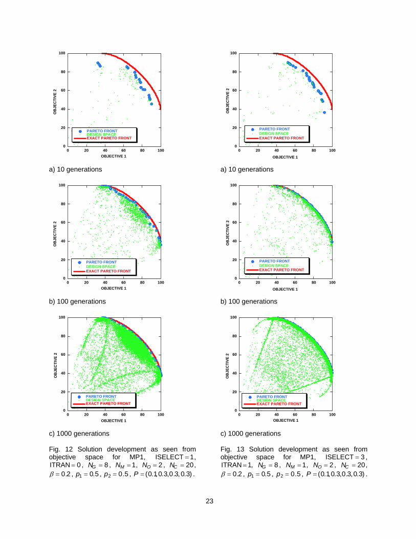
c) 1000 generations Fig. 12 Solution development as seen from objective space for MP1, ISELECT = 1,

, , , , ITRAN = 0 NG = 8 NM = 1 NO = 2 NC = 20, β = 0.2 , p , p , P . 1 = 0.5 2 = 0.5 = (0.1,0.3,0.3,0.3)

0

20

40

60

80

100

0 20 40 60 80 100

PARETO FRONTDESIGN SPACEEXACT PARETO FRONT

OB

JEC

TIVE

2

OBJECTIVE 1

a) 10 generations

0

20

40

60

80

100

0 20 40 60 80 100

PARETO FRONTDESIGN SPACEEXACT PARETO FRONT

OB

JEC

TIVE

2

OBJECTIVE 1

b) 100 generations

0

20

40

60

80

100

0 20 40 60 80 100

PARETO FRONTDESIGN SPACEEXACT PARETO FRONT

OB

JEC

TIVE

2

OBJECTIVE 1

c) 1000 generations Fig. 13 Solution development as seen from objective space for MP1, ISELECT = 3 , ITRAN = 1, NG = 8 , , , NM = 1 NO = 2 NC = 20, β = 0.2 , p1 = 0.5 , p2 = 0.5 , .P = (0.1,0.3,0.3,0.3)

23

Confirmation of this observation can be obtained by looking at the development of the pareto front at different GA generation levels. This is done for two cases in Figs. 12 and 13. Figure 12 shows pareto front development at the 10, 100 and 1000 generation levels for the ISELECT , = 1 ITRAN = 0 case. Figure 13 shows pareto front development at the same generation levels for the ISELECT = 3 , ITRAN = 1 case. Three sets of data are displayed in each plot: the exact pareto front as a solid red line, the approximate pareto front as a series of blue circles and the design space—all solutions explored to that point—as a series of small green dots. As can be seen from Figs. 12 and 13, the ISELECT = 3 , ITRAN = 1 case develops its pareto front much more rapidly than the ISELECT , = 1 ITRAN = 0 case. In fact, the approximate pareto front at 100 generations for the ISELECT = 3 , ITRAN = 1 case (Fig. 13b) more accurately represents the exact pareto front than the approximate pareto front at 1000 generations for the ISELECT = 1, case (Fig. 12c). This behavior is in general agreement with the convergence history results that are displayed in Fig. 11, which utilized the area error norm.

ITRAN = 0

From Fig. 11 it can be seen that the three convergence history curves that utilize the transformation procedure ( ITRAN ) display better convergence performance than the three convergence history curves that do not use the transformation procedure ( ITRAN

= 1= 0 ). In particular, after an error drop of two

orders of magnitude, the difference in the number of function evaluations is more than an order of magnitude. More importantly, the slope on each of the ITRAN = 1 convergence history curves is steeper than any of the ITRAN curves, indicating that the method speed up will only increase as the GA process converges further.

= 0

The effect of the selection algorithm (ISELECT) and the gene space transformation procedure (ITRAN) on GA convergence efficiency for MP2 is presented in Fig. 14. Results for all three selection algorithms and both values of ITRAN are presented. In each case the pareto front error using the area error norm is plotted against the number of function evaluations. Because of the effective increase in design space noise caused by using N , all convergence history curves were averaged over 100 solutions, i.e.,

. M = 32

NSEED = 100

10-1

100

101

102

103

104

101 102 103 104 105

ISLECT ITRAN 1 0 1 1 2 0 2 1 3 0 3 1

PAR

ETO

FR

ON

T ER

RO

R

NUMBER OF FUNCTION EVALUATIONS

Fig. 14 Pareto front convergence histories for different ISLECT and ITRAN values, all other GA and design space parameters held fixed, MP2, , , , NSEED = 100 NG = 8 NM = 32 NO = 2 ,

, NC = 20 β = 0.1, , and .

p1 = 0.5 p2 = 0.1P = (0.1,0.3,0.3,0.3)

10-1

100

101

102

103

104

101 102 103 104 105

ISELECT ITRAN NM

1 0 1 1 0 32 3 1 1 3 1 32

PAR

ETO

FR

ON

T ER

RO

R

NUMBER OF FUNCTION EVALUATIONS

Fig. 15 Pareto front convergence histories for different ISLECT, ITRAN and N values, all other GA and design space parameters held fixed, MP1 and MP2, NSEED ,

M

= 100 NG = 8 , NO = 2 , NC = 20, β = 0.1, p , p1 = 0.5 2 = 0.1 and P = (0.1,0.3,0.3,0.3) .

24

For this case the results that utilize bin selection are clearly superior to the results that utilize either greedy selection or tournament selection. In addition, the ITRAN = 1 results when used in conjunction with bin selection are more efficient. Selected convergence history results from Fig. 11a (rerun with NSEED = 100 ) and Fig. 14—the fastest and slowest curves from each figure—are cross-plotted versus each other in Fig. 15. This allows a quantitative look at what the N parameter does to GA convergence. As can be seen, the faster results—ISELECT , —are only slightly inconvenienced by , whereas the slower results—ISELEC

M= 3 ITRAN = 1 NM = 32

T= 1, ITRAN —suffer from the existence of so many local extrema. = 0 The effect of the selection algorithm (ISELECT) and the gene space transformation procedure (ITRAN) on GA convergence efficiency for MP3 is presented in Figs. 16-18. Results for all three selection algorithms and both transformation variations are included. For each case presented in Fig. 16, the pareto front error using the area error norm is plotted against the number of function evaluations. All convergence history curves are averaged over 100 cases, i.e., NSEED = 100 . As seen from Fig. 16, the ISELECT= 3 , ITRAN = 1 and ISELECT= 3 , ITRAN = 0 schemes are still the most efficient, but now, there is less variation in convergence efficiency over all of the GA variations plotted. Overall the total error drop over 100,000 function evaluations ranged from about one-and-a-half orders of magnitude to a little less than two orders of magnitude. For MP1 and MP2 the total error drop over the same number of function evaluations ranged from about one to about four orders of magnitude. Generally, the convergence efficiency performance for the slower schemes across MP1, MP2 and MP3 was about the same. The faster schemes for MP1 and MP2, however, suffered dramatically when they were applied to MP3. The reason for this is most likely associated with MP3’s nonlinear side constraint, which produces a discontinuous and mildly convoluted pareto front.

10-3

10-2

10-1

100

101 102 103 104 105

ISELECT ITRAN 1 0 1 1 2 0 2 1 3 0 3 1

PAR

ETO

FR

ON

T ER

RO

R

NUMBER OF FUNCTION EVALUATIONS

Fig. 16 Pareto front convergence histories for different ISLECT and ITRAN values, all other GA and design space parameters held fixed, MP3, NSEED = 100 , NG = 2 , NO = 2 , , NC = 20 β = 0.2 , p1 = 0.5 ,

and P . p2 = 0.1 = (0.1,0.3,0.3,0.3) Comparisons between the computed and the exact pareto fronts superimposed on the numerically generated design space for MP3 are presented in Figs. 17 and 18. Two different cases, corresponding to

, ITRAN and ISELECT , IISELECT = 3 = 0 = 3 TRAN = 1, are included. In both cases the computed pareto front is represented with red circular symbols and the exact pareto front is represented with green dots. The design space data—which includes all solutions that were evaluated during the course of GA iteration and that did not violate one of the side constraints—are plotted using a series of black dots.

25

Note that both cases produce good approximations to the exact pareto front. The design space for the

case is approximately laid out within a triangle—one side along the pareto front, the other two along the x and x directions. The ITRANITRAN = 0

1 = constant 2 = constant = 1 case design space is more so flattened against the pareto front. This is a direct result of the gene-space transformation, as the 45° line that stretches from the pareto front endpoints becomes the preferred direction.

0

0.2

0.4

0.6

0.8

1

1.2

0 0.2 0.4 0.6 0.8 1 1.2

COMP PARETO FRONTEXACT PARETO FRONT

OB

JEC

TIVE

2

OBJECTIVE 1

a) Comparison of the computed and exact pareto fronts

0

0.2

0.4

0.6

0.8

1

1.2

0 0.2 0.4 0.6 0.8 1 1.2

COMP PARETO FRONTDESIGN SPACE

OB

JEC

TIVE

2

OBJECTIVE 1

b) Computed pareto front in relation to the computed design space Fig. 17 Pareto front comparisons for MP3, 2500 generations, ISELECT = 3 , , ITRAN = 0 NG = 2 ,

, N , NO = 2 C = 20 β = 0.1, p , p1 = 0.5 2 = 0.1 and . P = (0.1,0.3,0.3,0.3)

0

0.2

0.4

0.6

0.8

1

1.2

0 0.2 0.4 0.6 0.8 1 1.2

COMP PARETO FRONTEXACT PARETO FRONT

OB

JEC

TIVE

2OBJECTIVE 1

a) Comparison of the computed and exact pareto fronts

0

0.2

0.4

0.6

0.8

1

1.2

0 0.2 0.4 0.6 0.8 1 1.2

COMP PARETO FRONTDESIGN SPACE

OB

JEC

TIVE

2

OBJECTIVE 1

b) Computed pareto front in relation to the computed design space Fig. 18 Pareto front comparisons for MP3, 2500 generations, ISELECT = 3 , , ITRAN = 1 NG = 2 , NO = 2 , NC = 20, β = 0.1, p , p1 = 0.5 2 = 0.1 and P = (0.1,0.3,0.3,0.3) .

26

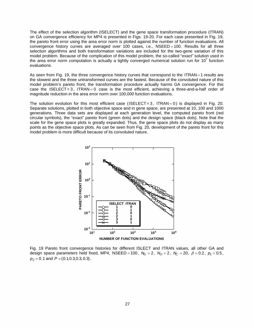
The effect of the selection algorithm (ISELECT) and the gene space transformation procedure (ITRAN) on GA convergence efficiency for MP4 is presented in Figs. 19-20. For each case presented in Fig. 19, the pareto front error using the area error norm is plotted against the number of function evaluations. All convergence history curves are averaged over 100 cases, i.e., NSEED = 100 . Results for all three selection algorithms and both transformation variations are included for the two-gene variation of this model problem. Because of the complication of this model problem, the so-called “exact” solution used in the area error norm computation is actually a tightly converged numerical solution run for 107 function evaluations. As seen from Fig. 19, the three convergence history curves that correspond to the ITRAN results are the slowest and the three untransformed curves are the fastest. Because of the convoluted nature of this model problem’s pareto front, the transformation procedure actually harms GA convergence. For this case the ISELECT , case is the most efficient, achieving a three-and-a-half order of magnitude reduction in the area error norm over 100,000 function evaluations.

= 1

= 3 ITRAN = 0

The solution evolution for this most efficient case ( ISELECT= 3 , ITRAN = 0 ) is displayed in Fig. 20. Separate solutions, plotted in both objective space and in gene space, are presented at 10, 100 and 1000 generations. Three data sets are displayed at each generation level, the computed pareto front (red circular symbols), the “exact” pareto front (green dots) and the design space (black dots). Note that the scale for the gene space plots is greatly expanded. Thus, the gene space plots do not display as many points as the objective space plots. As can be seen from Fig. 20, development of the pareto front for this model problem is more difficult because of its convoluted nature.

10-3

10-2

10-1

100

101

102

101 102 103 104 105

ISELECT ITRAN 1 0 1 1 2 0 2 1 3 0 3 1

PAR

ETO

FR

ON

T ER

RO

R

NUMBER OF FUNCTION EVALUATIONS

Fig. 19 Pareto front convergence histories for different ISLECT and ITRAN values, all other GA and design space parameters held fixed, MP4, NSEED = 100 , NG = 2 , NO = 2 , , NC = 20 β = 0.2 , p1 = 0.5 ,

and P . p2 = 0.1 = (0.1,0.3,0.3,0.3)

27

-8

-6

-4

-2

0

2

-10 -9 -8 -7

PARETO FRONTEXACT PARETO FRONTDESIGN SPACE

OB

JEC

TIVE

2

OBJECTIVE 1

a) Objective space, 10 generations.

-8

-6

-4

-2

0

2

-10 -9 -8 -7

PARETO FRONTEXACT PARETO FRONTDESIGN SPACE

OB

JEC

TIVE

2

OBJECTIVE 1

c) Objective space, 100 generations.

-8

-6

-4

-2

0

2

-10 -9 -8 -7

PARETO FRONTEXACT PARETO FRONTDESIGN SPACE

OB

JEC

TIVE

2

OBJECTIVE 1

e) Objective space, 1000 generations.

-1.2

-1

-0.8

-0.6

-0.4

-0.2

0

0.2

-1.2 -1 -0.8 -0.6 -0.4 -0.2 0 0.2

PARETO FRONTEXACT PARETO FRONT

GEN

E 2

GENE 1

b) Gene space, 10 generations.

-1.2

-1

-0.8

-0.6

-0.4

-0.2

0

0.2

-1.2 -1 -0.8 -0.6 -0.4 -0.2 0 0.2

PARETO FRONTEXACT PARETO FRONT

GEN

E 2

GENE 1

d) Gene space, 100 generations.

-1.2

-1

-0.8

-0.6

-0.4

-0.2

0

0.2

-1.2 -1 -0.8 -0.6 -0.4 -0.2 0 0.2

PARETO FRONTEXACT PARETO FRONT

GEN

E 2

GENE 1

f) Gene space, 1000 generations.

Fig. 20 Computed pareto fronts in objective and gene space at selected levels of convergence, MP4, ISELECT = 3 , ITRAN , N , N , N= 0 G = 2 O = 2 C = 20, β = 0.2 , p1 = 0.5 , p2 = 0.1 and P . = (0.1,0.3,0.3,0.3)

28

Effect of modification operator parameter variation on GA convergence—The effect of the various modification operator parameters on GA convergence efficiency is studied in this section. In particular, three parameters will be considered, β , and p . The p1 2 β parameter is used to control the size of perturbations in the perturbation mutation operator. The p parameter is used to control the probability that any given gene will be perturbed in the same operator. The p parameter is used to control the probability that any given gene will be mutated using the global mutation modification operator. The number of chromosomes modified by these two operators is controlled by the third and fourth elements of the P vector, respectively. For all results in this section, P

1

2

= (0.1,0.3,0.3,0.3) . Thus, the perturbation mutation and global mutation operators are each used to update 30% of all chromosomes. Figure 21 shows the effect of β on GA convergence efficiency for each of the four model problems. In each case the pareto front error using the area error norm is plotted against the number of function evaluations. For all results in this section the bin selection algorithm without gene-space transformation is used, i.e., ISELECT = 3 , ITRAN . All convergence history curves are averaged over 100 cases. = 0

100

101

102

103

104

101 102 103 104 105

β = 0.01 = 0.02 = 0.05 = 0.1 = 0.2 = 0.5

PAR

ETO

FR

ON

T ER

RO

R

NUMBER OF FUNCTION EVALUATIONS

a) MP1, N . G = 8

100

101

102

103

104

101 102 103 104 105

β = 0.01 = 0.02 = 0.05 = 0.1 = 0.2 = 0.5

PAR

ETO

FR

ON

T ER

RO

R

NUMBER OF FUNCTION EVALUATIONS

b) MP2, N . G = 8

10-2

10-1

100

101

102

101 102 103 104 105

β = 0.01 = 0.02 = 0.05 = 0.1 = 0.2 = 0.5

PAR

ETO

FR

ON

T ER

RO

R

NUMBER OF FUNCTION EVALUATIONS

c) MP3, NG = 2 .

10-3

10-2

10-1

100

101 102 103 104 105

β = 0.01 = 0.02 = 0.05 = 0.1 = 0.2 = 0.5

PAR

ETO

FR

ON

T ER

RO

R

NUMBER OF FUNCTION EVALUATIONS

d) MP4, NG = 3 .

Fig. 21 Pareto front convergence histories for different model problems showing the effect of β variation on GA convergence efficiency, ISELECT = 3 , ITRAN = 0 , NSEED = 100 , , , NO = 2 NC = 20 p1 = 0.5 ,

and P . p2 = 0.1 = (0.1,0.3,0.3,0.3)

29

As can be seen from in Fig. 21, the convergence history curves associated with different values of β tend to cross each other. This trend exists for each model problem and is manifested by the fact that the optimal value of β varies as a function of convergence level. But the trend for which values are most efficient and which are least efficient changes across the various model problems. For MP1 and MP2, which have a simple, well-behaved pareto front, moderate values of β are most efficient for early convergence. As the final pareto front is approached, smaller and smaller perturbations are required for optimal convergence. This is the same trend observed for single-objective optimization problems as reported in Ref. 10. For MP3 and MP4, which have more complex pareto fronts, being either mildly convoluted or strongly convoluted, the smaller values of β are generally best for early convergence, and the larger values of β are generally best for late convergence. The precise reason for this trend is unclear, but it suggests that a GA approach that uses adjustable values of β might be attractive. Figure 22 shows the effect of p on GA convergence efficiency for each of the four model problems. In each case the pareto front error using the area error norm is plotted against the number of function evaluations. For all results in this section the bin selection algorithm without gene-space transformation is used, i.e., ISELECT , ITRAN , and all convergence history curves are averaged over 100 cases.

1

= 3 = 0

101

102

103

104

101 102 103 104 105

p1 = 0.05

= 0.1 = 0.2 = 0.5 = 1.0

PAR

ETO

FR

ON

T ER

RO

R

NUMBER OF FUNCTION EVALUATIONS

b) MP1, N . G = 8

101

102

103

104

101 102 103 104 105

p1 = 0.05

= 0.1 = 0.2 = 0.5 = 1.0

PAR

ETO

FR

ON

T ER

RO

R

NUMBER OF FUNCTION EVALUATIONS

b) MP2, N . G = 8

10-3

10-2

10-1

100

101 102 103 104 105

p1 = 0.05

= 0.1 = 0.2 = 0.5 = 1.0

PAR

ETO

FR

ON

T ER

RO

R

NUMBER OF FUNCTION EVALUATIONS

c) MP3, NG = 2

10-2

10-1

100

101

102

101 102 103 104 105

p1 = 0.05

= 0.01 = 0.2 = 0.5 = 1.0

PAR

ETO

FR

ON

T ER

RO

R

NUMBER OF FUNCTION EVALUATIONS

d) MP4, NG = 3

Fig. 22 Pareto front convergence histories for different model problems showing the effect of variation on GA convergence efficiency, ISELECT

p1= 3 , ITRAN = 0 , NSEED = 100 , , , NO = 2 NC = 20 β = 0.2 ,

and P . p2 = 0.1 = (0.1,0.3,0.3,0.3)

30

As can be seen from Fig. 22, the effect of p on GA convergence efficiency is small for MP1, MP2 and MP4 and only marginal for MP3. For MP1, MP2 and MP4, intermediate values of p are generally best, while for MP3 larger values are best.

1

1

Figure 23 shows the effect of p on GA convergence efficiency on two of the model problems—MP1 and MP4—the two model problems with the simplest pareto front and the most complex pareto front. In each case the pareto front error using the area error norm is plotted against the number of function evaluations. For each plot, results for ITRAN

2

= 0 and ITRAN = 1 are presented for just two values of p —0.0 and 1.0.

2

As can be seen in Fig. 23, the effect of p on GA convergence efficiency is negligible for all cases presented. Many other cases were run, which utilized different values of p . The effect of p on GA convergence efficiency was always negligible. This is in direct contrast with the single-objective results obtained in Ref. 10. For the single-objective results, the effect of p on GA convergence efficiency was also negligible for cases in which design space noise was nonexistent or small, but dramatic for cases in which the design space noise was significant. It can only be surmised that none of the cases attempted in this study possessed enough design space noise to demonstrate the effect of p on GA convergence efficiency.

2

2 2

2

2

100

101

102

103

104

101 102 103 104 105

ITRAN p2

0 0.05 0 1.0 1 0.05 1 1.0

PAR

ETO

FR

ON

T ER

RO

R

NUMBER OF FUNCTION EVALUATIONS

a) MP1, N . G = 8

10-2

10-1

100

101

102

101 102 103 104 105

ITRAN p2

0 0.05 0 1.0 1 0.05 1 1.0

PAR

ETO

FR

ON

T ER

RO

R

NUMBER OF FUNCTION EVALUATIONS

b) MP4, NG = 3 .

Fig. 23 Pareto front convergence histories for different model problems showing the effect of p variation on GA convergence efficiency, ISELEC

2T = 3 , NSEED = 100 , NO = 2 , NC = 20, β = 0.2 , p1 = 0.5 and

. P = (0.1,0.3,0.3,0.3) Effect of P vector variation on GA convergence—The effect of the P vector, which controls which modification operators are to be used in going from G to Gn n+1 , is studied in this section. Selected convergence history results for each of the model problems (MP1; MP2, MP3 and MP4) are displayed in Fig. 24. In each case convergence history results for the baseline value of the P vector,

, along with an assortment of other P vector values designed to systematically emphasize each of the later three modification operators—random average crossover, perturbation mutation and global mutation—are displayed. For all results in this section the bin selection algorithm without gene-space transformation is used, i.e., ISELEC

P = (0.1,0.3,0.3,0.3)

T = 3 , ITRAN = 0 . All convergence history curves are averaged over 100 cases, i.e., NSEED = 100 .

31

As can be seen from Fig. 24 the effect of different P vector values on GA convergence is not as large as for some of the other parameters studied. The variation in efficiency between the best and worst convergence history curves—as measured by the ratio of the number of function evaluations at fixed error—is generally between three and five for each of the model problems. In addition, the asymptotic convergence rates for each P vector for each model problem are almost identical, thus indicating that the relative efficiency comparisons will continue to smaller values of error. Additional trends across each of the model problems are also observable. The two best convergence history curves for each model problem are always associated with the baseline P vector and the P vector that emphasizes the perturbation mutation operator—P = (0.1, 0.1,0.7,0.1) . The P vector that emphasizes global mutation— —is always associated with the worst convergence history efficiency.

P = (0.1, 0.1,0.1,0.7)

101

102

103

104

101 102 103 104 105

P = (0.1, 0.3, 0.3, 0.3)P = (0.1, 0.7, 0.1, 0.1)P = (0.1, 0.1, 0.7, 0.1)P = (0.1, 0.1, 0.1, 0.7)

PAR

ETO

FR

ON

T ER

RO

R

NUMBER OF FUNCTION EVALUATIONS

a) MP1, N . G = 8

101

102

103

104

101 102 103 104 105

P = (0.1, 0.3, 0.3, 0.3)P = (0.1, 0.7, 0.1, 0.1)P = (0.1, 0.1, 0.7, 0.1)P = (0.1, 0.1, 0.1, 0.7)

PAR

ETO

FR

ON

T ER

RO

R

NUMBER OF FUNCTION EVALUATIONS

b) MP2, N . G = 8

10-3

10-2

10-1

100

101 102 103 104 105

P = (0.1, 0.3, 0.3, 0.3)P = (0.1, 0.7, 0.1, 0.1)P = (0.1, 0.1, 0.7, 0.1)P = (0.1, 0.1, 0.1, 0.7)

PAR

ETO

FR

ON

T ER

RO

R

NUMBER OF FUNCTION EVALUATIONS

c) MP3.

10-2

10-1

100

101

102

101 102 103 104 105

P = (0.1, 0.3, 0.3, 0.3)P = (0.1, 0.7, 0.1, 0.1)P = (0.1, 0.1, 0.7, 0.1)P = (0.1, 0.1, 0.1, 0.7)

PAR

ETO

FR

ON

T ER

RO

R

NUMBER OF FUNCTION EVALUATIONS

d) MP4, NG = 3 .

Fig. 24 Pareto front convergence histories for different model problems showing the effect of P vector variation on GA convergence efficiency, ISELECT = 3 , ITRAN = 0 , NSEED = 100 , , NO = 2 NC = 20, β = 0.2 , p and p . 1 = 0.5 2 = 0.1

32

Effect of number of genes on GA convergence—The effect of the number of genes used to define the design space (N ) is studied in this section. Selected convergence history results for two of the model problems (MP1 and MP4) are displayed in Fig. 25. For MP1 N is varied from 2 to 64 and for MP4 N is varied from 2 to 8. For all results in this section the bin selection algorithm without gene-space transformation is used, i.e., ISELECT ,

G

G G

= 3 ITRAN = 0 . All convergence history curves are averaged over 100 cases, i.e., NSEED . = 100 As can be seen from Fig. 25, the effect of N on GA convergence is dramatic. The key thing to look at in Fig. 25 is the slope of each curve, i.e., how much does each curve drop during the course of 100,000 function evaluations? Not surprisingly, as N increases, the rate at which the GA converges decreases. Thus, in choosing a design space discretization, it is imperative to select a parameterization that leads to the smallest number of decision variables as possible.

G

G

100

101

102

103

104

101 102 103 104 105

NG = 2

= 4 = 8 = 16 = 32 = 64

PAR

ETO

FR

ON

T ER

RO

R

NUMBER OF FUNCTION EVALUATIONS

a) MP1.

10-3

10-2

10-1

100

101

102

103

101 102 103 104 105

NG = 2

= 3 = 8

PAR

ETO

FR

ON

T ER

RO

R

NUMBER OF FUNCTION EVALUATIONS

b) MP4.

Fig. 25 Pareto front convergence histories for different model problems showing the effect of N variation on GA convergence efficiency, ISELEC

GT = 3 , ITRAN = 0 , NSEED = 100 , , , NO = 2 NC = 20 β = 0.2 ,

, p and P . p1 = 0.5 2 = 0.1 = (0.1,0.3,0.3,0.3) Effect of number of chromosomes on GA convergence efficiency—For all GA algorithm variations studied in this report, the number of chromosomes in each population, N , is held fixed over the entire optimization process. Nevertheless, the value of N is a user specified parameter that can have an impact on GA convergence. Quantification of this impact for the four model problems is presented in Fig. 26. In each case the error in the pareto front using the area error norm is plotted against the number of function evaluations. For all results in this section the bin selection algorithm without gene-space transformation is used, i.e., ISELECT ,

C

C

= 3 ITRAN = 0 . All convergence history curves are averaged over 100 cases, i.e., NSEED . = 100 As can be seen from Fig. 26, especially Figs. 26a and b, which are associated with the simple pareto fronts of MP1 and MP2, the initialization penalty increases with increasing values ofN . Nevertheless, the asymptotic convergence is not affected by the value of N . In particular, after enough function evaluations, somewhere around 5000-10000, all of the convergence history results for a given model problem collapse to a single curve. Generally, the smaller values of N produced the fastest convergence. This has a significant implication for massively parallel applications and suggests that GA optimization approaches can be parallelized on virtually any number of processors with an extremely high degree of efficiency.

C

C

C

33

101

102

103

104

101 102 103 104 105

NC = 20

= 50 = 100 = 200 = 500

PAR

ETO

FR

ON

T ER

RO

R

NUMBER OF FUNCTION EVALUATIONS

a) MP1, N . G = 8

101

102

103

104

101 102 103 104 105

NC = 20

= 50 = 100 = 200 = 500

PAR

ETO

FR

ON

T ER

RO

R

NUMBER OF FUNCTION EVALUATIONS

b) MP2, N . G = 8

10-3

10-2

10-1

100

101 102 103 104 105

NC = 20

= 50 = 100 = 200 = 500

PAR

ETO

FR

ON

T ER

RO

R

NUMBER OF FUNCTION EVALUATIONS

c) MP3, NG = 2 .

10-2

10-1

100

101

102

101 102 103 104 105

NC = 20

= 50 = 100 = 200 = 500

PAR

ETO

FR

ON

T ER

RO

R

NUMBER OF FUNCTION EVALUATIONS

d) MP4, NG = 3 .

Fig. 26 Pareto front convergence histories for different model problems showing the effect of number of chromosomes, , on GA convergence efficiency, ISELECNC T = 3 , ITRAN = 0 , , NSEED = 100 NO = 2 ,

, p and P . p1 = 0.5 2 = 0.1 = (0.1,0.3,0.3,0.3)

Conclusions A genetic algorithm (GA) optimization procedure, with several selection algorithm options and a new gene-space transformation procedure, has been presented. The new algorithm is especially designed for multi-objective optimization problems. It uses real-number encoding to represent all design space decision variables as genes and populations of fixed size to go from generation to generation. Four modification operators are utilized to advance from one generation to the next. They include passthrough, random average crossover, perturbation mutation and mutation. The standard output for this approach is a pareto front, which includes the best solutions from each objective, as well as a range of non-dominated “tradeoff” solutions in between.

34

The GA optimization procedure converged to the global pareto front optimum for every case attempted, demonstrating robustness and wide applicability. In some cases convergence was achieved quickly, while in other cases convergence was much slower. Four model problems with different design space characteristics were used to systematically study the effects of the various GA parameters on convergence performance. The following specific conclusions were obtained: Of the three selection algorithms tested, greedy, tournament and binning, the latter produced the most efficient convergence across all of the problems studied. The gene-space transformation procedure was successful for model problems with simple pareto fronts, achieving improvements in convergence efficiency. It was moderately successful for model problems with mildly convoluted pareto fronts and displayed a degradation in convergence performance for pareto fronts that were strongly convoluted. Key design space features that tended to diminish GA convergence performance were large numbers of genes and design spaces that were highly convoluted. The fact that these areas would slow convergence is intuitive. A more difficult less intuitive area to assess is the effect of GA parameters on convergence performance. The conclusions in this area are presented by looking at each GA parameter separately. In general, GA parameter values had only a small to moderate effect on GA convergence efficiency. The perturbation mutation parameter controlling size of the perturbation mutations (β ) displayed a crossover behavior for each model problem studied, with one value of β more efficient during early convergence and another value more efficient during late convergence. The perturbation mutation probability (p ) generally had a small effect on GA convergence efficiency with moderate values producing the best convergence. The global mutation probability (p ) had a negligible effect on GA convergence efficiency for all cases tested. Lastly, the P vector had a moderate effect on convergence efficiency with the default value—P —or values that emphasized the perturbation mutation operator being the best.

1

2

= (0.1,0.3,0.3,0.3)

The number of chromosomes used in each generation, N , had a small effect on GA convergence efficiency for all situations studied. Initially, the larger values of N seemed to possess an initialization penalty that suggested their convergence efficiency would be degraded, but asymptotically, the larger values of N produced the same convergence rate as smaller values of for all model problems studied. This suggests that the GA optimization procedure would be extremely attractive for implementation on massively parallel computers.

C

C

C NC

References

1. Goldberg, D. E., “Genetic Algorithms in Search, Optimization and Machine Learning,” Addison-

Wesley, Reading, MA, 59-88, 1989. 2. Davis, L., “Handbook of Genetic Algorithms,” Van Nostrand Reinhold, New York, 1991. 3. Beasley, D., Bull, D. R. and Martin, R. R., “An Overview of Genetic Algorithms: Part 1,

Fundamentals,” University Computing, Vol. 15, No. 2., 1993, pp. 58-69. 4. Beasley, D., Bull, D. R. and Martin, R. R., “An Overview of Genetic Algorithms: Part 2, Research

Topics,” University Computing, Vol. 15, No. 4., 1993, pp. 170-181. 5. Deb, Kalyanmoy, “Multi-Objective Genetic Algorithms: Problem Difficulties and Construction of Test

Problems,” Evolutionary Computation, Vol. 7, No. 3, 1999, pp. 205-230. 6. Van Veldhuizen, David and Lamont, Gary, “Multiobjective Evolutionary Algorithms: Analyzing the

State-of-the-Art,” Evolutionary Computation, Vol. 8, No. 2, 2000, pp. 125-147.

35

7. Jiménez, José, Cuesta, Pedro and Abderramán, Jesús, “Mixed Strategy in Genetic Algorithms:

Domain’s Reduction and Multirecombination,” European Congress on Computational Methods in Applied Sciences and Engineering, ECCOMAS 2000, Barcelona, Spain, Sept. 2000.

8. Obayashi, S. and Tsukahara, T., “Comparison of Optimization Algorithms for Aerodynamic Shape

Design,” AIAA J., Vol. 35, 1997, pp. 1413-1415. 9. Bock, K.-W., “Aerodynamic Design by Optimization,” Paper 20, AGARD CP-463, 1990. 10. Holst, T. L. and Pulliam, T. H., Evaluation of Genetic Algorithm Concepts using Model Problems,

Part I: Single-Objective Optimization, NASA TM in preparation, 2003. 11. Zitzler, E., Thiele, L. Laumanns, M., Fonseca, C. M. and da Fonseca, V. G., “Performance

Assessment of Multiobjective Optimizers: An analysis and Review,” IEEE Transactions on Evolutionary Computation, Vol. 7, No. 2, April 2003, pp. 117-132.

12. Deb, K., Pratap, A. and Meyarivan, T., “Constrained Test Problems for Multi-Objective Evolutionary

Optimization,” Proceedings of the First International Conference on Evolutionary Multi-Criterion Optimization, March 7-9, 2001, Zurich, Switzerland, pp. 284-298.

13. Van Veldhuizen, D., “Multiobjective Evolutionary Algorithms: Classification, Analyses, and New

Innovations,” AFIT/DS/ENG/99-01, June 1999. 14. Lohn, J. D., Kraus, W. F. and Haith, G. L., “Comparing a Coevolutionary Genetic Algorithm for

Multiobjective Optimization, Proceedings of the 2002 IEEE Congress on Evolutionary Computation, May 2002, pp. 1157-1162.

15. Laumanns, M., Thiele, L., Deb, K. and Zitzler, E., “On the Convergence and Diversity-Preservation

Properties of Multi-Objective Evolutionary Algorithms,” Swiss Federal Institute of Technology (ETH), Zürich, Switzerland, TIK Report No. 108, June 2001.

16. Deb, K., Mohan, M. and Mishra, S., “A Fast Multi-Objective Evolutionary Algorithm for Finding Well-

Spread Pareto-Optimal Solutions,” Kanpur Genetic Algorithms Laboratory (KANGAL), KanGAL Report No. 2003002, Feb. 2003.

17. Knowles, J. D. and Corne, D. W., “Approximating the Nondominated Front Using the Pareto

Archived evolution Stategy,” Evolution Computation, Vol. 8, No. 2, 2000, pp. 149-172. 18. Knowles, J. and Corne, D., “Properties of an Adaptive Archiving Algorithm for Storing Nondominated

Vectors,” IEEE Transactions on Evolutionary Computation, Vol. 7, No. 2, April 2003, pp. 100-116. 19. Parmee, I. C., Cvetkovic, D., Gonham, C. R. and Mitchell, D., “Towards Interactive Evolutionary

Design Systems for the Satisfaction of Multiple and Changing Objectives, European Congress on Computational Methods in Applied Sciences and Engineering, ECCOMAS 2000, Barcelona, Spain, Sept. 2000.

20. Marco, N, Désidéri, J.-A. and Lanteri, S., “Multi-Objective Optimization in CFD by Genetic

Algorithms,” Institut National de Recherche en Informatique et en Automatique, Research Report No. 3686, April 1999.

21. Naujoks, B., Willmes, L., Haase, W., Bäck, T. and Schütz, M., “Multi-Point Airfoil Optimization Using

Evolution Strategies,” European Congress on Computational Methods in Applied Sciences and Engineering, ECCOMAS 2000, Barcelona, Spain, Sept. 2000.

36

22. Quagliarella, D. and Della Cioppa, A., “Genetic Algorithms Applied to the Aerodynamic Design of

Transonic Airfoils,” AIAA Paper 94-1896-CP, 1994. 23. Vicini, A. and Quagliarella, D., “Inverse and Direct Airfoil Design Using a Multiobjective Genetic

Algorithm,” AIAA J., Vol. 35, 1997, pp. 1499-1505. 24. Hämäläinen, J., Mäkinen, A., Tarvainen, P. and Toivanen, J., “Evolutionary Shape Optimization in

CFD with Industrial Applications,” European Congress on Computational Methods in Applied Sciences and Engineering, ECCOMAS 2000, Barcelona, Spain, Sept. 2000.

25. Epstein, B. and Peigin, S., “A Robust Hybrid GA/ROM Approach to multiogjective constrained

Optimization in Aerodynamics,” 16th AIAA Computational Fluid Dynamics Conference, Orlando, Florida, AIAA Paper No. 2003-4092, June 2003.

26. Anderson, M., Burkhalter, J. and Jenkins, R., “Missile Aerodynamic Shape Optimization Using

Genetic Algorithms,” J. of Spacecraft and Rockets, Vol. 37, No. 5, Sept.-Oct. 2000, pp. 663-669. 27. Anderson, M. and Gebert, G., “Using Pareto Genetic Algorithms for Preliminary Subsonic Wing

Design,” AIAA Paper No. 96-4023-CP, 1996. 28. Sasaki, D, Obayashi, S. and Nakahashi, K., “Navier-Stokes Optimization of Supersonic Wings with

Four Design Objectives Using Evolutionary Algorithm,” AIAA Paper No. 2001-2531, 2001. 29. Oyama, A., “Multidisciplinary Optimization of Transonic Wing Design Based on Evolutionary

Algorithms Coupled with CFD Solver,” European Congress on Computational Methods in Applied Sciences and Engineering, ECCOMAS 2000, Barcelona, Spain, Sept. 2000.

30. Ng, K. Y., Tan, C. M., ray, T. and Tsai, H. M., “Single and Multiobjective Wing Planform and Airfoil

Shape Optimization using a Swarm Algorithm,” 41st Aerospace Sciences meeting and Exhibit, Reno, Nevada, AIAA Paper No. 2003-45, Jan. 2003.

31. Obayashi, S., Yamaguchi, Y. and Nakamura, T., “Multiobjective Genetic Algorithm for

Multidisciplinary Design of Transonic Wing Planform,” J. of Aircraft, Vol. 34, 1997, pp. 690-693. 32. Oyama, A. and Liou, M.-S., “Multiobjective Optimization of Rocket Engine Pumps Using Evolutionary

Algorithm,” AIAA Paper No. 2001-2581, June 2001. 33. Benini, E., “Three-Dimensional Multi-Objective Design Optimization of a Transonic Compressor

Rotor,” 16th AIAA Computational Fluid Dynamics Conference, Orlando, Florida, AIAA Paper No. 2003-4090, June 2003.

34. Oyama, A. and Liou, M., “Multiobjective Optimization of a Multi-Stage Compressor Using

Evolutionary Algorithm,” AIAA Paper No. 2002-3535, 2002. 35. Giotis, A. P., Giannakoglou, K. C. and Périaux, J., “A Reduced-Cost Multi-Objective Optimization

Method Based on the Pareto Front Technique, Neural Networks and PVM,” European Congress on Computational Methods in Applied Sciences and Engineering, ECCOMAS 2000, Barcelona, Spain, Sept. 2000.

36. Tursi, S., “Transonic Wing Optimization Combining Genetic Algorithm and Neural Network,” 21st

AIAA Applied Aerodynamics Conference, Orlando, Florida, AIAA Paper No. 2003-3787, June 2003. 37. Vicini, A. and Quagliarella, D., “Airfoil and Wing Design Through Hybrid Optimization Strategies,”

AIAA Paper No. 98-2729, 1998.

37

38. Brown, M. and Smith, R. E., “Effective Use of Directional Information in Multi-Objective Evolutionary

Computation,” Genetic and Evolutionary Computation Conference (GECCO 2003), July 2003. 39. Oyama, A., “Wing Design Using Evolutionary Algorithms,” PhD Thesis, Dept. of Aeronautics and

Space Engineering, Tohoku University, Senadi, Japan, March 2000. 40. Houck, G. R., Joines, J. A. and Kay, M. G., “A Genetic Algorithm for Function Optimization: A Matlab

Implementation,” North Carolina State University-IE, TR 95-09, 1995. 41. Michalewicz, Z., Genetic Algorithms + Data Structures = Evolution Programs, AI Series, Springer-

Verlag, New York, 1994. 42. Noble, B., Applied Linear Algebra, Prentice Hall, Englewood Cliffs, New Jersey, 1969, pp. 314-318. 43. Tanaka, M., “GA-based Decision Support System for Multi-Criteria Optimization,” Proceedings of the

International Conference on Systems, Man and Cybernetics-2, pp. 1556-1561, 1995. 44. Kursawe, F., “A Variant of Evolution Strategies for Vector Optimization,” Parallel Problem Solving

from Nature, 1496, Lecture Notes in Computer Science, edited by H.-P. Schwefel and R. Männer, Springer-Verlag, Berlin, Germany, October 1990, pp. 193-197.

45. Fonseca, C. M. and Fleming, P. J., “On the Performance Assessment and Comparison of Stochastic

Multiobjective Optimizers,” Parallel Problem Solving From Nature IV, edited by Voigt, H.-M., Ebeling, W., Rechenberg, I. and Schwefel, H.-P., Springer, Berlin, Germany, 1995, pp. 584-593.

38

REPORT DOCUMENTATION PAGE

8. PERFORMING ORGANIZATION REPORT NUMBER

10. SPONSORING/MONITORING AGENCY REPORT NUMBER

Form Approved

OMB No. 0704-0188

12b. DISTRIBUTION CODE12a. DISTRIBUTION/AVAILABILITY STATEMENT

7. PERFORMING ORGANIZATION NAME(S) AND ADDRESS(ES)

4. TITLE AND SUBTITLE 5. FUNDING NUMBERS

6. AUTHOR(S)

1. AGENCY USE ONLY (Leave blank)

9. SPONSORING/MONITORING AGENCY NAME(S) AND ADDRESS(ES)

2. REPORT DATE 3. REPORT TYPE AND DATES COVERED

15. NUMBER OF PAGES

16. PRICE CODE

20. LIMITATION OF ABSTRACT19. SECURITY CLASSIFICATION OF ABSTRACT

18. SECURITY CLASSIFICATION OF THIS PAGE

17. SECURITY CLASSIFICATION OF REPORT

14. SUBJECT TERMS

13. ABSTRACT (Maximum 200 words)

Standard Form 298 (Rev. 2-89)Prescribed by ANSI Std. Z39-18298-102

NSN 7540-01-280-5500

Public reporting burden for this collection of information is estimated to average 1 hour per response, including the time for reviewing instructions, searching existing data sources,gathering and maintaining the data needed, and completing and reviewing the collection of information. Send comments regarding this burden estimate or any other aspect of thiscollection of information, including suggestions for reducing this burden, to Washington Headquarters Services, Directorate for information Operations and Reports, 1215 JeffersonDavis Highway, Suite 1204, Arlington, VA 22202-4302, and to the Office of Management and Budget, Paperwork Reduction Project (0704-0188), Washington, DC 20503.

11. SUPPLEMENTARY NOTES

Unclassified Unclassified

Unclassified — UnlimitedSubject Category - 59 Distribution: NonstandardAvailability: NASA CASI (301) 621-0390

A-0311046

NASA/TM–2003-212813

December 2003

Ames Research CenterMoffett Field, CA 94035-1000

National Aeronautics and Space AdministrationWashington, DC 20546-0001

302-15-31

42

Evaluation of Genetic Algorithm Concepts Using Model ProblemsPart II: Multi-Objective Optimization

Terry L. Holst and Thomas H. Pulliam

A genetic algorithm approach suitable for solving multi-objective optimization problems is described andevaluated using a series of simple model problems. Several new features including a binning selectionalgorithm and a gene-space transformation procedure are included. The genetic algorithm is suitable forfinding pareto optimal solutions in search spaces that are defined by any number of genes and that containany number of local extrema. Results indicate that the genetic algorithm optimization approach is flexible inapplication and extremely reliable, providing optimal results for all optimization problems attempted. Thebinning algorithm generally provides pareto front quality enhancements and moderate convergence effi-ciency improvements for most of the model problems. The gene-space transformation procedure provides alarge convergence efficiency enhancement for problems with non-convoluted pareto fronts and a degrada-tion in efficiency for problems with convoluted pareto fronts. The most difficult problems—multi-modesearch spaces with a large number of genes and convoluted pareto fronts—require a large number of func-tion evaluations for GA convergence, but always converge.

Optimization, Genetic algorithms, Multi-objective

Technical Memorandum

Point of Contact: Terry Holst, Ames Research Center, MS T27B-1, Moffett Field, CA 94035-1000 (650) 604-6032

Unclassified