evaluation of multilayer perceptron (mlp) and self ... · universidade do porto ... instituto de...
TRANSCRIPT

1
Evaluation of Multilayer Perceptron and Self-Organizing Map
Neural Network Topologies applied on Microstructure
Segmentation from Metallographic Images
Victor Hugo Costa Albuquerque1, Auzuir Ripardo de Alexandria2, Paulo César Cortez3,
João Manuel R. S. Tavares1
1Instituto de Engenharia Mecânica e Gestão Industrial (INEGI) / Faculdade de Engenharia da
Universidade do Porto (FEUP), Departamento de Engenharia Mecânica e Gestão Industrial
(DEMEGI), Rua Dr. Roberto Frias, S/N, 4200-465, Porto, Portugal
Emails: {victor.albuquerque, tavares}@fe.up.pt
2Centro Federal de Educação Tecnológica (CEFETCE), NSMAT, Indústria, Av. Treze de
Maio, 2081, 60040-531, Fortaleza, Ceará, Brasil
Email: [email protected]
3Universidade Federal do Ceará, Departamento de Engenharia de Teleinformática, Caixa
Postal 6007, 60.755-640, Fortaleza, Ceará, Brasil
Email: [email protected]
Corresponding author: Prof. João Manuel R. S. Tavares Instituto de Engenharia Mecânica e Gestão Industrial (INEGI) Faculdade de Engenharia da Universidade do Porto (FEUP), Departamento de Engenharia Mecânica e Gestão Industrial (DEMEGI) Rua Dr. Roberto Frias, s/n 4200-465 PORTO PORTUGAL Telf.: +315 22 5081487, Fax: +315 22 5081445 Email: [email protected] Url: www.fe.up.pt/~tavares

2
Abstract
Artificial neuronal networks have been used intensively in many domains to
accomplish different computational tasks. One of these tasks is the segmentation of objects in
images, like to segment microstructures from metallographic images, and for that goal several
network topologies were proposed. This paper presents a comparative analysis between
Multilayer Perceptron and Self-Organizing Map topologies applied to segment
microstructures from metallographic images. The multilayer perceptron neural network
training was based on the backpropagation algorithm, that is a supervised training algorithm,
and the self-organizing map neural network was based on the Kohonen algorithm, being thus
an unsupervised network. Sixty samples of cast irons were considered for experimental
comparison and the results obtained by multilayer perceptron neural network were very
similar to the ones resultant by visual human inspection. However, the results obtained by
self-organizing map neural network were not so good. Indeed, multilayer perceptron neural
network always segmented efficiently the microstructures of samples in analysis, what did not
occur when self-organizing map neural network was considered. From the experiments done,
we can conclude that multilayer perceptron network is an adequate tool to be used in Material
Science fields to accomplish microstructural analysis from metallographic images in a fully
automatic and accurate manner.
Keywords: Nondestructive testing and evaluation; image processing and analysis; pattern
recognition; multilayer perceptron and self-organizing map neural networks; cast irons;
metallographic images; material sciences.

3
1 Introduction
The use of artificial neural networks is quite common in Artificial Intelligence and
Pattern Recognition domains. In particularly, they have been used in applications that involve
shapes recognition with a high degree of parallelism, considerable classification speed and
important capacity to learn through examples [1]. The smallest unit of an artificial neural
network is the artificial neuron which is a mathematical representation of a natural neuron that
compounds living neural systems.
Some domains in which artificial neural networks have been widely applied can be
found in Material Sciences. For example, they can be employed in welding control [2], to
obtain relations between process parameters and correlations in Charpy impact tests [3], to
obtain the composition of ceramic matrices [3], in the modeling of alloy elements [4], to
estimate welding parameters in pipeline welding [5], in the modeling of microstructures and
mechanical properties of steel [6], to model the deformation mechanism of titanium alloy in
hot forming [7], for the prediction of properties of austempered ductile iron [8], to predict the
carbon content and the grain size of carbon steels [9], to build models for predicting flow
stress and microstructures evolution of a hydrogenized titanium alloy [10], to perform
segmentation and quantification of microstructures in metals from images [11, 12], to classify
internal damages in steels working in creep service [13], and to perform the optimal
binarization of images in the morphological analysis of ductile cast iron [14].
Artificial neural networks have been also extremely applied to perform image
segmentation tasks. Actually, many Computational Vision systems are developed based on
artificial neural networks, essentially because of their main characteristics, like robustness to
noisily input data or outliers, execution speed and possibility to be parallel implemented.
In this work were considered two neural network topologies widely used in pattern
recognition applications: Multilayer Perceptron and Self Organizing Map, based on

4
backpropagation (supervised) and Kohonen (non-supervised) algorithms, respectively. In
particularly, these neural architectures were used and compared in the automatic segmentation
of the microstructures of metallic materials from metallographic images. To evaluate
experimentally their efficiency, it was used samples of nodular, malleable and gray cast irons.
Those materials were selected mainly due to their widespread use in industrial applications, as
in, for example, machine base structures, lamination cylinders, main bodies of valves and
pumps and gear elements.
This paper is organized as follows. In next section, some essential aspects of
Multilayer Perceptron neural networks are reviewed and the topology used is presented. The
equivalent is done in third section considering Self Organizing Map neural networks. In next
section the experimental work accomplished is explained and results are discussed. In last
section the main conclusions are presented.
2 Multilayer Perceptron Neural Network
A human brain is composed by about ten billion neurons and their organization is of
high structural and functional complexity. These units are densely interconnected, which
results in a very complex architecture and with an intelligence level that was not yet achieved
by any artificial system. Several mathematical models have been developed to represent
neurons and their interconnection. In this direction, artificial neural networks have appeared
as an attempt to reproduce human brain potentialities, specially its learning ability [15].
The first neuron mathematical model was proposed by McCulloch and Pitts [16]. It
has a binary output and several inputs, each one with a different excitatory or inhibitory gain.
These gains are known as synaptic weights (or only weights). Input signal values and
associated weights determine the neuron output [15].

5
Thus, perceptron or artificial neuron is the mathematical model of a neuron cell and
the basic unit that compounds an artificial neural network. Perceptron architecture consists of
a set of n inputs (xi), each one associated to a weight (wi) and an activation function (fi).
Perceptrons can be organized to form a layer, in which all perceptrons are linked to the same
inputs but have distinct outputs. This kind of network is designated as a perceptron network.
Perceptron networks can achieve good performances only when the pattern to be recognized
is linearly separable [15]; therefore, they should not be used to solve complex classification
problems involving non-linearly separable patterns, instead multilayer perceptron networks
can be used.
2.1 Multilayer perceptron networks architecture
Multilayer perceptron networks are formed by an input layer (Xi), one or more
intermediary or hidden layers (HL) and an output layer (Y). A weight matrix (W) can be
defined for each of these layers. This artificial neuronal network topology can solve
classification problems involving non-linearly separable patterns and can be used as a
universal function generator [15].
Multilayer perceptron networks have two distinct phases: training and execution. With
this network topology, it is impossible to use directly the usual delta rule [15] for the training
phase, since this rule does not permit weight recalculation for hidden layers. Therefore, the
most widely used algorithm for multilayer perceptron networks training is the
backpropagation and its variants. This learning approach is more complex than the one for a
perceptron network and it is of the type supervised [16].
2.1.1 Backpropagation Algorithm

6
Standard backpropagation algorithm is one of the most used algorithms to train
neuronal networks [15, 17]. This algorithm is applied by initializing the weights randomly
and presenting examples to the neuronal network as an input signal. Then, this signal is
propagated through the hidden layers and achieves the output layer where the network outputs
are obtained. Afterwards, the weights (w) are modified according to equation:
.η=∆ ijw )(kjδ )(ksj , (1)
where localjij efk .)( =δ to 1
( ) ( ), output layer and. , otherwise
j jllocalj
jp p
d k s ke
pw δ −
−= ∑
,
and i is the current neuron input, j is the neuron, l is the current layer and, s is neuron output,
d is the desired output, fi is a derivative activation function. Finally, this procedure is repeated
until the error is less than a previously adopted threshold value.
This algorithm presents some disadvantages like, for example, during the search for a global
minimum, the surface where the error derivative is almost null can be achieved and remain
there forever. The convergence of the neural network can be very time-consuming since the
trajectory of the initial weights set towards the final one is randomly defined.
2.2 Topology of the multilayer perceptron network used
In this work was used a multilayer perceptron with two layers. Since the main task was
the segmentation of material microstructures from metallographic images, it was used to
classify the pixels of a metallographic image as belonging to one of these material
microstructures: graphite, pearlite or ferrite. For that, we choose a 3/2/3 (three inputs, two
perceptrons in hidden layer and three perceptrons in output layer) topology. For each input
was assigned one color component (R, G and B) of each pixel of the input image to be
segmented. Each output was assigned to the three possible pixel classifications: graphite,
pearlite or ferrite. The number of perceptrons used in the hidden layer was established using

7
the method proposed by Yin, Liu and Han [18]. Finally, to perform microstructures
quantification, for each microstructure segmented, the associated pixels were counted and the
relative percent value for the whole image was calculated.
As already referred, to train the artificial network was used backpropagation algorithm
and the examples considered were microstructure pixels chosen from representative input
images. It should be noted that the training phase just needed to be done once for each kind of
metallic material to be segmented.
3 Self-organizing map neural networks
Self-organizing map neural network is a topology proposed by Kohonen [19] that
consists in a feedforward neural network that uses a non-supervised training. This model is
usually built by a neuron layer disposed linearly (1D) or through a plane (2D) and is classified
as a self-organizing map since the neurons are disposed in an one-dimensional or bi-
dimensional reticulated, as shown in figure 1. In this figure is illustrated a self-organizing
neural network with a 1D topology and a bi-dimensional network in a squared topology with
nine neurons organized in a 3x3 array.
When a pattern is presented to a self-organizing map neural network, their neurons
compete among themselves in order to determine the one that has the best response to the
input pattern. The neuron that generates the least Euclidian distance between the input and
weights vector is the chosen winner, and it has its weights adjusted to respond better to the
input pattern. Kohonen network, then, has the characteristic of modifying internally so that
the neurons respond better to a determined input pattern [20].
Concerning self-organizing non-supervised learning model, not only the winner
neuron but also the ones in its neighborhood have their weights adjusted, as is explained in
the next section. This paradigm is based on the theory that the cells from brain cortex are
8
anatomically arranged in function of its stimulus originated from sensors that are directly
connected to them [20].
Each neuron of a self-organizing neural network represents an output. Another
characteristic of this network topology is that its neurons are totally connected (synaptic
links), so that if there are ten inputs, each neuron has ten inputs, each one linked to a point in
the input layer. Then, each synaptic connection has a weight so that if they are ten input
points, and should be three neurons in the network, then we should be thirty connections (ten
for each neuron) and consequently, thirty synaptic weights (ten for each neuron).
3.1 Neighborhood
A neuron in a self-organizing map network has a set of neighbors that can be
topologically organized in regions to have the best response to a given stimulus. This
characteristic is similar to the one that occurs in human brain, where, depending on the
activity that is happening, there are some neural centers of more intensified activity.
In the beginning of the training step, the set of neighbors is large, but it decreases
along time, while the network organizes itself. In fact, for its better organization, the
neighborhood begins wide and decreases monotonically, because if the neighborhood begins
very small, comparing to the whole map, the network does not become globally in order [20].
Usually, at the end of the process, neighborhood radius must be null and only the winner has
its weights adjusted.
Neighborhood weight adjustment permits that neurons near to the winner have good
conditions to dispute with the same during next iterations, improving in this way the
competition for the best network learning.
3.2 Neuron adaptation

9
Neuron adaptation consists in weight adjustment, looking for response improvement to
determined stimulus. This process is fundamental for the formation of an ordered network.
The first step to achieve weight adjustment is to determine the winner neuron. So, the winner
will be the neuron that presents the least Euclidean distance dt(n) between an input pattern and
its weights, calculated as:
∑=
−=I
1i
2))i(t,nw)i(tx()n(td , (2)
where xt(i) is the ith input vector component at time t, wn,t(i) is the ith weights vector
component of a neuron n at time t, i is the input and weight index of a network with I inputs
and dt(n) is Euclidean distance of neuron n at time t.
Euclidian distance, as presented in equation 2, is the sum of squared differences
between each input and its correspondent weight. In fact, the least Euclidean distance
represents the neuron which weight value is the most similar to input value presented [20]. In
this way, in each iteration, the neuron that has the least Euclidian distance and its neighbors
must have their weights adjusted to have a better response to that input, while the other
neurons remain equal. Weight adaptation at next instant t + 1 is a simple process. It consists in
taking the difference between vectors X (input) and W (weights) and sum a fraction of this
difference to the weight vector at time t (actual). Neighbor weights are adjusted using the
same principle, expressed by:
2))()().(()()1( twtxtatwtw nsnn −+=+ , (3)
where as(t) is the learning rate and corresponds to a fraction of difference between X and W
that is summed to W. So that, 0 < as < 1 [15].
Usually as(t) (equation 3) is initialized with a high value (around one), and
successively decreases, following any rule or function, until its value achieves approximately

10
zero. Then, map ordering that takes place in the beginning of training is affected by a large
neighborhood radius and by a high as(t) value.
3.3 Iterations
The number of iterations or epochs corresponds to the number of times that the input
patterns are presented to the network. On each epoch, it must be presented all input data. For
each pattern a winner neuron is determined. Then, its weights and the weights of its neighbors
are adjusted. After the last pattern is presented, a new epoch begins and all input data must be
presented again [19].
3.4 Training algorithm for a self-organizing map neural network
The self-organizing training algorithm used can be described as follows [19]:
1. specify the number of epochs;
2. initialize the network weights using random values;
3. specify the initial neighborhood radius for each neuron (it is recommended to use
the whole network as initial radius);
4. present an input to the network;
5. calculate the output for each neuron, using Euclidean distance between input and
network weight;
6. select the winner neuron;
7. adjust winner weights and the ones of its neighbors;
8. if still there are neighbors, then decrease neighborhood radius;
9. if still there are input data, then go to step 4;
10. increment number of epochs and if allowed maximum number of epochs was still
not achieved, then go to step 4 and present all input data again.

11
It is important that the initial weight values are different from each other and much
smaller than input data. If the weights are initialized with values similar to input data, then the
network has the tendency to choose specific winners, avoiding its self organization.
3.5 Winner neuron
After network training, we can label each neuron according to the pattern it classifies.
By this way, if, for example, a network is classifying objects, and the winner neuron
represents a determined object, this neuron can be labeled with that object name.
Nevertheless, many neurons can classify the same object. In fact, this can occur because of its
neighborhood situation. If this case happens, then there will be more than a neuron with the
same label and a post-processing step can be necessary.
3.6 Topology of the self-organizing map neural network used
The applied self-organizing map topology was a 1-D self-organizing network and its
main task was to perform the segmentation of material microstructures from metallographic
images. Thus, self-organizing map neuronal network was used to recognize the pixels of a
metallographic image that belong to each of these material microstructures: graphite, pearlite
or ferrite. Hence, we choose a three neurons network having three inputs on each of them. To
each input is assigned one color component of input image pixels (R, G and B). Each neuron
is assigned to three possible pixel classifications: graphite, pearlite or ferrite. To perform
microstructures quantification, segmented pixels were counted and the associated percent was
calculated. Kohonen training algorithm was used to train the network and the examples used
were microstructure pixels obtained automatically from representative input images.

12
4 Results and discussion
The aim of this work was to segment material microstructures from metallographic
images; for this, we used two types of artificial neural network topologies to identify the
following microstructures: graphite, pearlite and ferrite. The experimental results were
obtained applying multilayer perceptron and self-organizing map neural networks on samples
of nodular, malleable and gray cast irons. Here we present a comparative analysis between
these two artificial neural network topologies in the automatic segmentation of metal
microstructures from metallographic images. For that comparison, we consider the analysis
presented by the Albuquerque et al. [12], which validated the quality of the segmentation and
quantification results obtained by the multilayer perceptron network on the microstructures of
cast irons from metallographic images. In the referred work, the results obtained by the
multilayer perceptron network were very similar to the ones obtained by visual human
inspection and better than the results obtained using a commercial system that is awfully
common and well accepted in the microstructures analysis area. Thus, we adopted the results
obtained by the multilayer perceptron network as a reference basis.
In the previous sections, we describe the neuronal network topologies to identify three
different microstructures in input images, however both networks were only used to identify
two classes, where one class indicates the presence of graphite (associated with black color in
the input images) and the other class refers to the presence of pearlite or ferrite (associated
with the gray color in the input images). The reason for the association pearlite/ferrite in one
class was because we were not able to visually distinguish these two microstructures in the
input images, which could affect the further results analysis.
The experimental images considered here had size of 640 x 480 pixels, the training
phase was performed once by an experimented operator considering four representative
images of each iron considered. This number of training images was defined in function of the

13
number of microstructures involved, and the training images were manually elected by the
operator through visual inspection. The same operator accomplished the experimental results
analysis and comparison. It should be noticed that different results could be obtained if the
networks were trained using different sets of training images. In other words, the quality of
the results accomplished depends on the quality of the image training set used and of each
image considered. That is, if all microstructures involved are or not properly represented in
the training images, the samples were or not well metallographic prepared or the images were
or not appropriately acquired as, for example, using inadequate contrast and illumination
conditions, the results quality can be affected.
In the training of the multilayer perceptron network, the backpropagation algorithm
was employed, adopting a learning rate of 0.1, a moment rate of 0.001, and as stopping
criterion the number of epochs equal to 2500 or an absolute error not greater than 0.01. In the
training of the self-organizing map network was used the Kohonen algorithm, adopting a
learning rate of 0.1 and as stopping criterion the number of epochs equal to 2500.
In table 1, are shown the results obtained using multilayer perceptron and self-
organizing map neural networks in the case of the nodular cast iron. It should be noticed that
the results obtained are similar, presenting a minimum difference of 1.00% and a maximum of
5.59%, for samples 20 and 17, respectively. Moreover, it can be noticed that the multilayer
perceptron network presented an average of graphite equal to 12.09% and pearlite or ferrite to
87.91% and that self-organizing map network presented 15.35% and 84.65% of graphite and
pearlite or ferrite, respectively, being the difference average equal to 3.26%.
Figures 2 (a), (b) and (c), present an original image of a nodular cast iron, and the
images resulting of the segmentation process accomplished using multilayer perceptron and
self-organizing map neuronal networks, respectively. These images are the ones that
presented the major difference in the results obtained by the two neuronal networks.

14
Additionally, images of figures 2 (d), (e) and (f), are the ones that presented the minor
difference.
It should be noticed that the segmentation done using multilayer perceptron network is
more accurate than the one obtained using the self-organizing map network, since part of the
pearlite or ferrite was erroneously segmented and classified as graphite by self-organizing
map network. This fact is the main justification for the existing difference in the results
obtained.
In table 2, the results of the segmentation done using multilayer perceptron and self-
organizing map networks on samples of a gray cast iron are presented. These results were the
most dissimilar for the studied irons, presenting a minimum difference of 1.86% and
maximum of 14.70%, for samples 15 and 18, respectively. Moreover, it can be noticed that
multilayer perceptron network presented an average of graphite equal to 10.28% and of
pearlite or ferrite to 89.62%, and that self-organizing map network presented 19.62% and
80.38% of graphite and of pearlite or ferrite, respectively, being the difference average
between the two neural networks equal to 9.24%.
Figures 3 (a), (b) and (c), present the original image of a gray cast iron, and the
resulting images of the segmentation done using multilayer perceptron and self-organizing
map neural networks, respectively. These images are the ones that presented the minor
difference between results obtained by the two neural networks. Additionally, images of
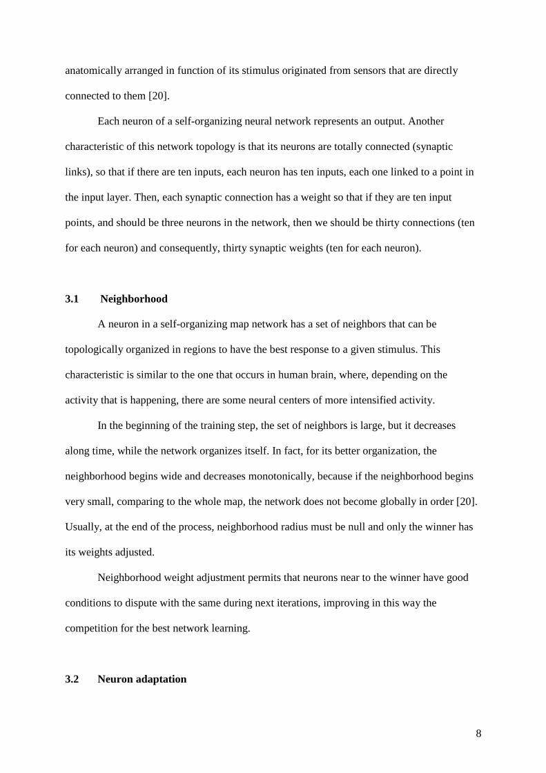
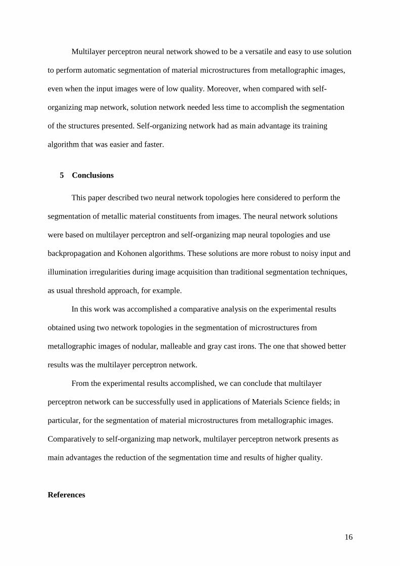
figures 3 (d), (e) and (f), are the ones that presented the major difference.
Analyzing the results obtained, one can conclude that the segmentations accomplished
using multilayer perceptron and self-organizing map neural network topologies are similar for
sample 1. Relatively to sample 11, the segmentation done by visual inspection is very similar
to the one obtained using multilayer perceptron network which not occurs with self-
organizing map network, because pearlite or ferrite was erroneously segmented as graphite.

15
In table 3, the results obtained by the segmentation done using multilayer perceptron
and self-organizing map methods on a malleable cast iron are presented. These are the most
similar results obtained by the two neural networks on all samples analyzed, presenting a
minimal difference of 1.54% and maximum of 5.62% for samples 3 and 19, respectively.
Moreover, it can be noticed that multilayer perceptron network presented an average of
graphite equal to 14.98% and of pearlite or ferrite to 85.02% and self-organizing map network
presented 17.70% and 82.30% of graphite and pearlite or ferrite, respectively, being the
involved difference average between the neural networks equal to 2.72%.
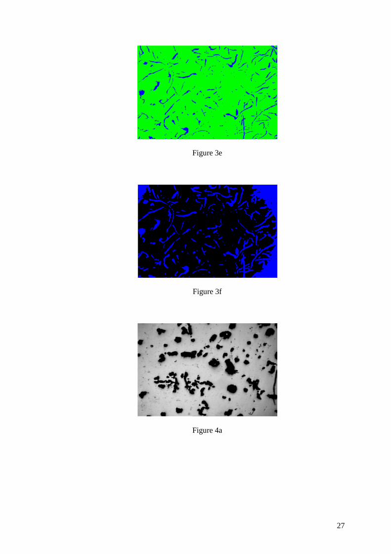
Figures 4 (a), (b) and (c), present an original image of a malleable cast iron and the
images resulting from the segmentation done using multilayer perceptron and self-organizing
map neural network, respectively. Notice that these images presented the minor difference
verified between the results obtained by the used networks. Additionally, the images of
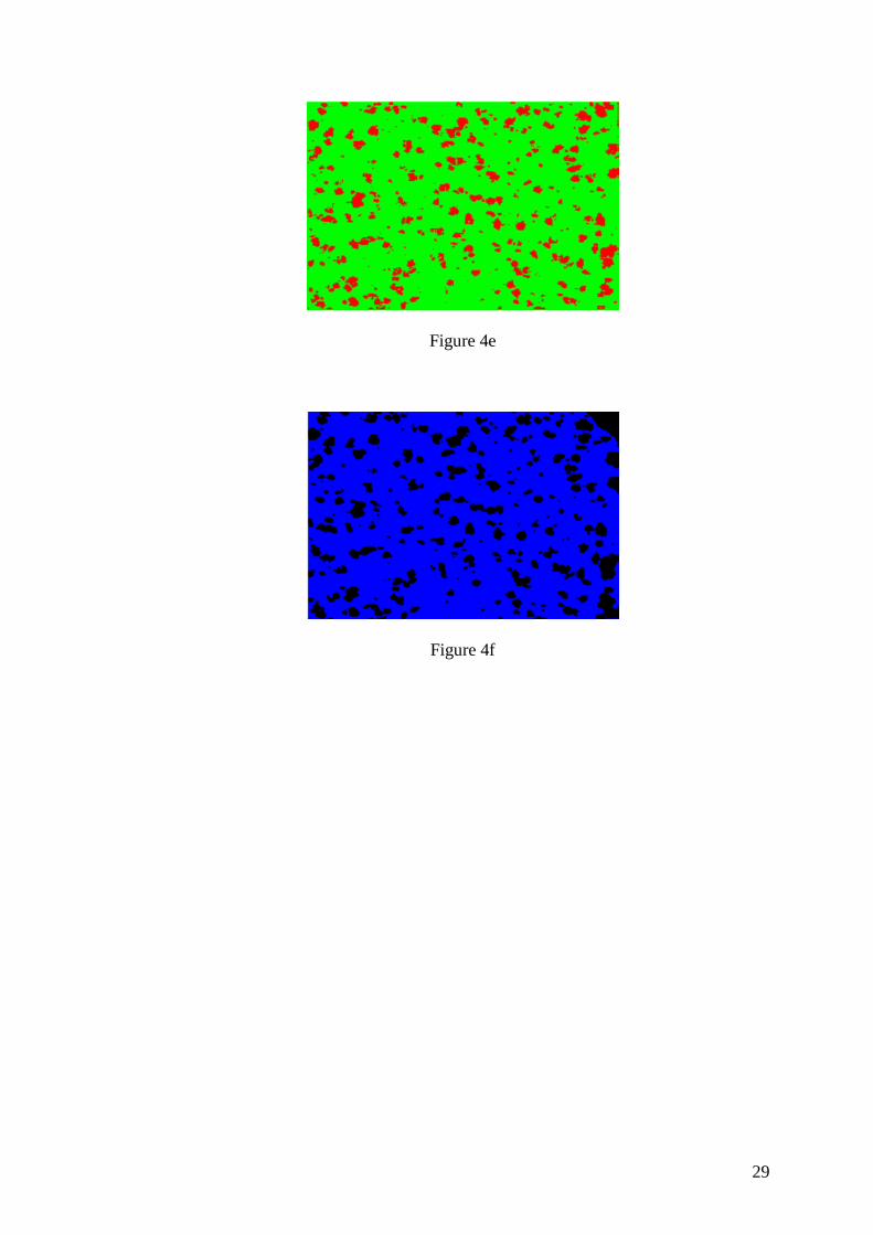
figures 4 (d), (e) and (f), presented the major difference.
Verifying the results obtained, it can be noticed that the segmentations performed
using multilayer perceptron and self-organizing map neural networks are analogous on
sample 3. For sample 19, the segmentations obtained are distinct, because self-organizing
map network segments great part of pearlite or ferrite as graphite (figure 4(f)). However, that
error is not verified when used multilayer perceptron network that segmented correctly the
graphite from the other two constituents.
In the results obtained by self-organizing map network on samples of nodular, gray
and, in particularly, malleable casting iron, we can verify its considerable difficulty to
segment graphite successfully when the background of the input image was not uniform.
However, multilayer perceptron network did not show this difficulty, and so it could get
segmentation results very effectively.
16
Multilayer perceptron neural network showed to be a versatile and easy to use solution
to perform automatic segmentation of material microstructures from metallographic images,
even when the input images were of low quality. Moreover, when compared with self-
organizing map network, solution network needed less time to accomplish the segmentation
of the structures presented. Self-organizing network had as main advantage its training
algorithm that was easier and faster.
5 Conclusions
This paper described two neural network topologies here considered to perform the
segmentation of metallic material constituents from images. The neural network solutions
were based on multilayer perceptron and self-organizing map neural topologies and use
backpropagation and Kohonen algorithms. These solutions are more robust to noisy input and
illumination irregularities during image acquisition than traditional segmentation techniques,
as usual threshold approach, for example.
In this work was accomplished a comparative analysis on the experimental results
obtained using two network topologies in the segmentation of microstructures from
metallographic images of nodular, malleable and gray cast irons. The one that showed better
results was the multilayer perceptron network.
From the experimental results accomplished, we can conclude that multilayer
perceptron network can be successfully used in applications of Materials Science fields; in
particular, for the segmentation of material microstructures from metallographic images.
Comparatively to self-organizing map network, multilayer perceptron network presents as
main advantages the reduction of the segmentation time and results of higher quality.
References

17
[1] S. Samarasinghe, Neural networks for applied sciences and engineering: from
fundamentals to complex pattern recognition, Auerbach Publications, 2006.
[2] H.K.D.H. Bhadeshia, Neural networks in materials science, ISIJ International 39(10): 966-
979, 1999.
[3] H.K.D.H. Bhadeshia, Neural networks and genetic algorithms in materials science and
engineering, Tata McGraw-Hill Publishing Company Ltd., India: 1-9, 2006.
[4] L. Miaoquana, X. Aiming, H. Weichao, W. Hairong, S. Shaobo and S. Lichuang,
Microstructural evolution and modelling of the hot compression of a TC6 titanium alloy,
Materials Characterization 49(3): 203-209, 2004.
[5] I. Kim, Y. Jeong, C. Lee and P. Yarlagadda, Prediction of welding parameters for pipeline
welding using an intelligent system, The International Journal of Advanced Manufacturing
Technology 22(9-10): 713-719, 2003.
[6] J. Kusiak and R. Kusiak, Modelling of microstructure and mechanical properties of steel
using the artificial neural network, Journal of Materials Processing Technology 127(1): 115-
121, 2002.
[7] X. Xiao-li and L. Miao-quan, Microstructure evolution model based on deformation
mechanism of titanium alloy in hot forming, Transactions of nonferrous metals society of
China 15(4): 749-753, 2005.
[8] R. Biernacki, J. Kozłowski, D. Myszka and M. Perzyk, Prediction of properties of
austempered ductile iron assisted by artificial neural network, Materials Science 12(1): 11-15,
2006.
[9] A. Abdelhay, Application of artificial neural networks to predict the carbon content and
the grain size for carbon steels, Egyptian Journal of Solids 25(2): 229-243, 2002.

18
[10] O. Wang, J. Lai and D. Sun, Artificial neural network models for predicting flow stress
and microstructure evolution of a hydrogenized titanium alloy, Key Engineering Materials
353-358: 541-544, 2007.
[11] V.H.C. Albuquerque, P.C. Cortez, A.R. Alexandria, W.M. Aguiar and E.M. Silva, Image
segmentation system for quantification of microstructures in metals using artificial neural
networks, Revista Matéria 12(2): 394-407, 2007.
[12] V.H.C. Albuquerque, P.C. Cortez, A.R. Alexandria and J.M.RS. Tavares, A new solution
for automatic microstructures analysis from images based on a backpropagation artificial
neural network, Nondestructive Testing and Evaluation 23(4): 273-283, 2008.
[13] L.A. Dobrzanski, M. Sroka and J. Dobrzanski, Application of neural networks to
classification of internal damages in steels working in creep service, Journal of Achievements
in Materials and Manufacturing Engineering 20(1-2): 303-305, 2007.
[14] A. de Santis, O. di Bartolomeo, D. Iacoviello, F. Iacoviello, Optimal binarization of
images by neural networks for morphological analysis of ductile cast iron, Pattern Analysis
and Applications 10(2): 125-133, 2007.
[15] S. Haykin, Neural Networks and Learning Machines. Prentice Hall, USA, 2009.
[16] W.S. McCullogh and W. Pitts, A logical calculus of the ideas immanent in nervous
activity, Neurocomputing: foundations of research book contents: 15-27, 1988.
[17] D. Plaut, S.J. Nowlan and G.E. Hinton, Experiments on learning by backpropagation.
Computer Science Department, Carnegie – Mellon University, Technical Report CMU-CS,
1986.
[18] X.C. Yin, C.P. Liu and Z. Han, Feature combination using boosting. Pattern Recognition
Letters 26(16): 2195-2205, 2005.
[19] T. Kohonen, Self-organized formation of topologically correct feature maps, Biological
Cybernetics 43(1): 59-69, 1982.

19
[20] T. Kohonen, Self-Organizing Maps. Springer Series in Information Sciences 30,
Springer-Verlag, Berlin, 2001.

20
FIGURES CAPTION
Figure 1: Two models for self-organizing map networks: a) 1-D and b) 2-D.
Figure 2: Two original images of a nodular cast iron, a) and d); resultant segmentation using
multilayer perceptron, b) and e), and self-organizing map, c) and f), neural networks.
Figure 3: Original images of a gray cast iron, a) and d); resultant images of the segmentation
done using multilayer perceptron, b) and e), and self-organizing map, c) and f), neural
networks.
Figure 4: Original image of a malleable cast iron, a) and d); resultant images of the
segmentation done using multilayer perceptron, b) and e), and self-organizing map, c) and f),
neural networks.

21
TABLES CAPTION
Table 1: Results obtained using multilayer perceptron (MLP) and Kohonen self-organizing
map based neural networks on samples of a nodular cast iron.
Table 2: Results obtained using multilayer perceptron (MLP) and Kohonen self-organizing
map (SOM) based neural networks on samples of a gray cast iron.
Table 3: Results obtained using multilayer perceptron (MLP) and Kohonen self-organizing
map (SOM) based neural networks on samples of a malleable cast iron.

22
Acknowledgments
To Federal Center of Technological Education of Ceará - CEFET CE, for the support
given for the accomplishment of this work, in particular to Mechanical Testing Laboratory
and to Teleinformatic Laboratory. The authors would like to thank also to CAPES for their
financial support.

23
FIGURES
Figure 1a
Figure 1b
Figure 2a

24
Figure 2b
Figure 2c
Figure 2d

25
Figure 2e
Figure 2f
Figure 3a

26
Figure 3b
Figure 3c
Figure 3d
27
Figure 3e
Figure 3f
Figure 4a

28
Figure 4b
Figure 4c
Figure 4d
29
Figure 4e
Figure 4f

30
TABLES
Table 1
Nodular cast iron
Samples MLP network (%) SOM network (%) Graphite Ferrite/Pearlite Graphite Ferrite/Pearlite
1 11.51 88.49 14.58 85.42 2 13.36 86.64 16.28 83.72 3 13.19 86.81 15.80 84.20 4 13.46 86.54 16.34 83.66 5 12.46 87.54 14.80 85.20 6 11.79 88.21 15.47 84.53 7 14.58 85.42 16.88 83.12 8 12.50 87.50 14.37 85.63 9 14.02 85.98 15.80 84.20 10 13.30 86.70 15.55 84.45 11 9.08 90.92 14.04 85.96 12 9.25 90.75 14.07 85.93 13 11.56 88.44 16.33 83.67 14 9.24 90.76 13.80 86.20 15 10.22 89.78 15.26 84.74 16 9.89 90.11 14.52 85.48 17 8.31 91.69 13.90 86.10 18 7.66 92.34 13.21 86.79 19 14.66 85.34 13.28 86.72 20 21.73 78.27 22.73 77.27
Average 12.09 87.91 15.35 84.65

31
Table 2
Gray cast iron
Samples MLP network (%) SOM network (%) Graphite Ferrite/Pearlite Graphite Ferrite/Pearlite
1 12.21 87.79 16.37 83.63 2 6.80 93.20 12.70 87.30 3 8.56 91.44 16.77 83.23 4 6.80 93.20 13.79 86.21 5 8.03 91.97 18.44 81.56 6 5.02 94.98 19.16 80.84 7 8.73 91.27 17.85 82.15 8 9.15 90.85 13.87 86.13 9 7.90 92.10 14.41 85.59 10 6.67 93.33 14.40 85.60 11 40.41 59.59 49.27 50.73 12 7.47 92.53 19.38 80.62 13 9.83 90.17 17.36 82.64 14 7.52 92.48 22.72 77.28 15 21.69 78.31 23.55 76.45 16 8.79 91.21 19.00 81.00 17 7.76 92.24 21.29 78.71 18 6.77 93.23 21.47 78.53 19 7.64 90.28 19.73 80.27 20 7.78 92.22 20.86 79.14
Average 10.28 89.62 19.62 80.38

32
Table 3
Malleable cast iron
Samples MLP network (%) SOM network (%) Graphite Ferrite/Pearlite Graphite Ferrite/Pearlite
1 18.95 81.05 20.57 79.43 2 15.71 84.29 17.73 82.27 3 14.96 85.04 16.50 83.50 4 14.00 86.00 15.63 84.37 5 15.16 84.84 17.28 82.72 6 16.07 83.93 18.32 81.68 7 19.11 80.89 20.76 79.24 8 19.22 80.78 22.17 77.83 9 15.64 84.36 17.60 82.40 10 17.64 82.36 19.40 80.60 11 11.84 88.16 16.82 83.18 12 12.04 87.96 17.32 82.68 13 13.72 86.28 18.84 81.16 14 14.06 85.94 18.07 81.93 15 11.83 88.17 16.07 83.93 16 11.40 88.60 16.19 83.81 17 11.30 88.70 15.54 84.46 18 10.68 89.32 15.15 84.85 19 21.05 78.95 15.43 84.57 20 15.27 84.73 18.57 81.43
Average 14.98 85.02 17.70 82.30