evaluation of ncep gfs clouds using a-train and arm...
TRANSCRIPT

Introduction Evaluation of NCEP GFS clouds
using A-train and ARM observations
Zhanqing Li, Hyelim Yoo Department of Atmospheric and Oceanic Science,
University of Maryland
Yu-Tai Hou, Shrinivas Moorthi, Brad Ferrier, Steve Lord NCEP/NOAA, College Park, MD
Howard B. Barker
Environment Canada, Toronto, Canada

Introduction Problems in representation of clouds
from Zhang et al. 2005
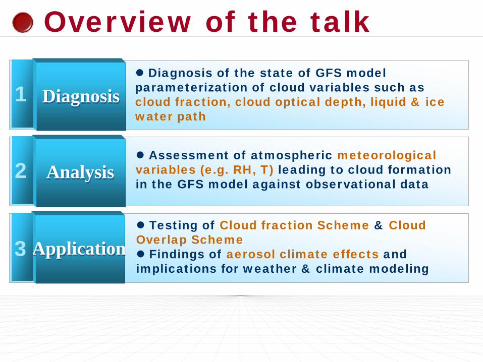
Overview of the talk
Analysis
Application
1
2
3
Diagnosis Diagnosis of the state of GFS model parameterization of cloud variables such as cloud fraction, cloud optical depth, liquid & ice water path
Assessment of atmospheric meteorological variables (e.g. RH, T) leading to cloud formation in the GFS model against observational data
Testing of Cloud fraction Scheme & Cloud Overlap Scheme Findings of aerosol climate effects and implications for weather & climate modeling
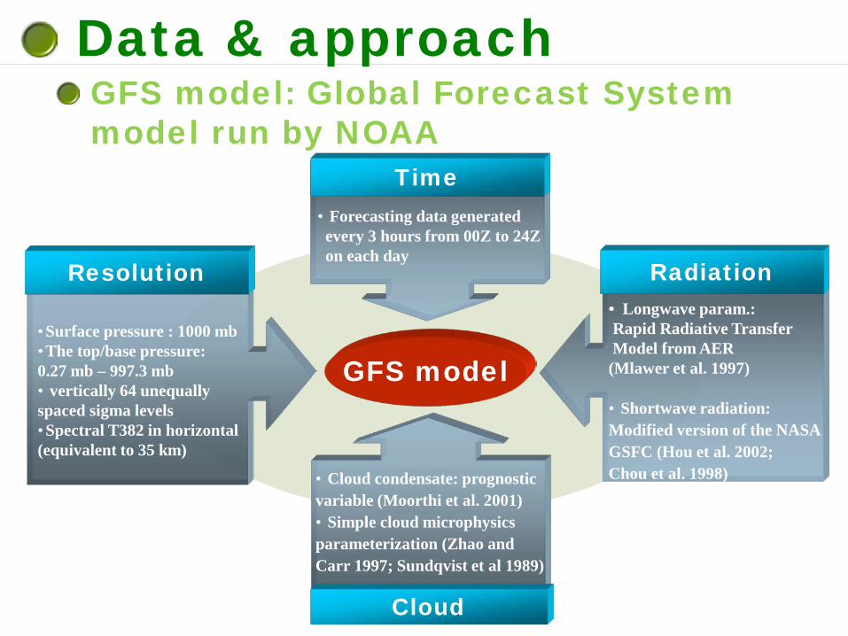
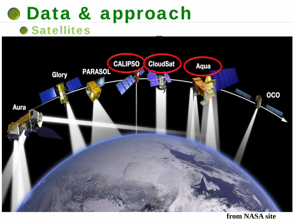
Data & approach GFS model: Global Forecast System model run by NOAA
GFS model • Surface pressure : 1000 mb • The top/base pressure: 0.27 mb – 997.3 mb • vertically 64 unequally spaced sigma levels • Spectral T382 in horizontal (equivalent to 35 km)
• Cloud condensate: prognostic variable (Moorthi et al. 2001) • Simple cloud microphysics parameterization (Zhao and Carr 1997; Sundqvist et al 1989)
Resolution
• Longwave param.: Rapid Radiative Transfer Model from AER (Mlawer et al. 1997) • Shortwave radiation: Modified version of the NASA GSFC (Hou et al. 2002; Chou et al. 1998)
Radiation
Cloud
Time • Forecasting data generated every 3 hours from 00Z to 24Z on each day
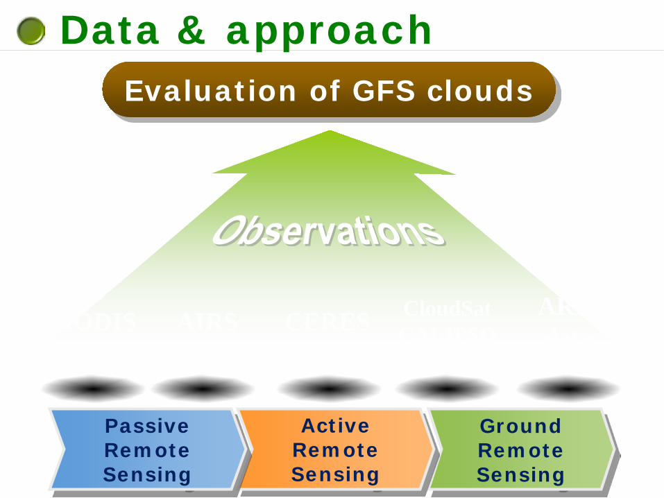
Data & approach Evaluation of GFS clouds
MODIS CERES AIRS CloudSat CALIPSO
ARM data
Ground Remote Sensing
Active Remote Sensing
Passive Remote Sensing

Satellite-retrieval algorithm Multi-layer cloud
mask code Twelve Cloud categories
0 Clear (no cloud retrieval) 1 Single low cloud (Tau < 3.6) 2 Single low cloud (3.6 < Tau < 23) 3 Single low cloud (Tau > 23) 4 Single mid cloud (Tau < 3.6) 5 Median mid cloud (3.6 < Tau < 23) 6 Thick mid cloud (Tau > 23) 7 Multi-layer mid cloud 8 Multi-layer high cloud 9 Marginal multi-layer (Tau2 < 1.5)
10 Single cirrus cloud (Tau < 3.6) 11 Single cirrocumulus cloud (3.6 < Tau < 23) 12 Deep convective cloud (Tau > 23)
Retrieve cloud top pressure, temperature, optical depth, emissivity for the first/second layer
Chang-Li algorithm (JAS & JCL, 2005)
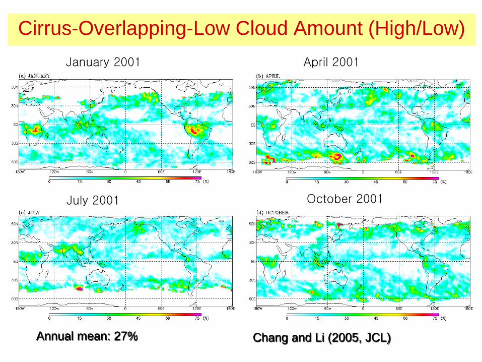
Cirrus-Overlapping-Low Cloud Amount (High/Low) January 2001 April 2001
July 2001 October 2001
Chang and Li (2005, JCL) Annual mean: 27%
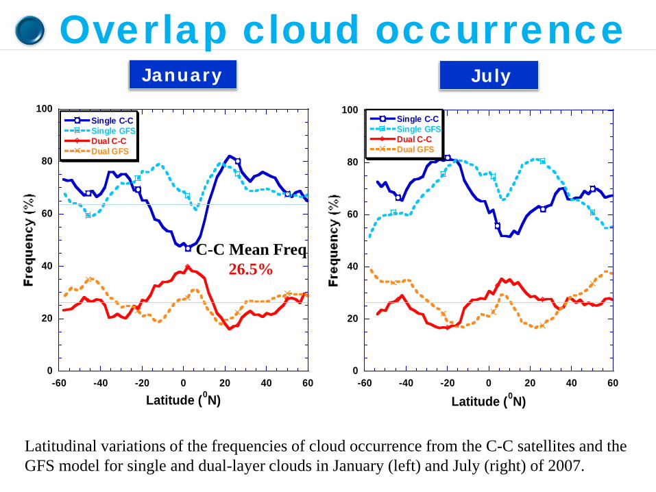
Overlap cloud occurrence
0
20
40
60
80
100
-60 -40 -20 0 20 40 60
Single C-CSingle GFSDual C-CDual GFS
Latitude (0N)
0
20
40
60
80
100
-60 -40 -20 0 20 40 60
Single C-CSingle GFSDual C-CDual GFS
Latitude (0N)
Latitudinal variations of the frequencies of cloud occurrence from the C-C satellites and the GFS model for single and dual-layer clouds in January (left) and July (right) of 2007.
January July
C-C Mean Freq 26.5%
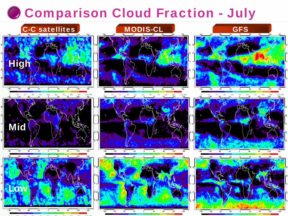
Comparison Cloud Fraction - July C-C satellites MODIS-CL GFS
High
Mid
Low

Comparison of clouds from radiosonde, radar and GFS radiosonde
GFS
ARSCL-M
ARSCL-L

Seasonal Variations of Clouds from Radiosonde, Radar and GFS
Radiosonde GFS Model Ground Radar

Comparison of radiation at the TOA CERES GFS
Outgoing SW
Outgoing LW
Net
Difference CERES-GFS
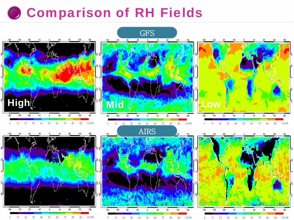
Comparison of RH Fields GFS
High High Mid
AIRS
Low
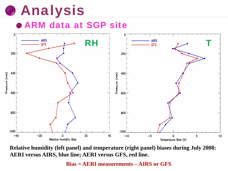
Analysis ARM data at SGP site
Relative humidity (left panel) and temperature (right panel) biases during July 2008: AERI versus AIRS, blue line; AERI versus GFS, red line.
Bias = AERI measurements – AIRS or GFS
RH T

Comparison of the Profiles of Relative Humidity & Temperature from Radiosonde, and GFS
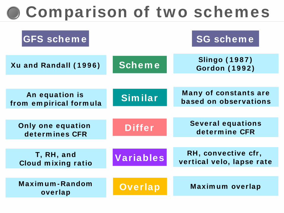
Comparison of two schemes
Scheme Xu and Randall (1996)
Similar
GFS scheme SG scheme
An equation is from empirical formula
Slingo (1987) Gordon (1992)
Many of constants are based on observations
Differ
Variables
Only one equation determines CFR
Several equations determine CFR
T, RH, and Cloud mixing ratio
RH, convective cfr, vertical velo, lapse rate
Overlap Maximum-Random overlap
Maximum overlap
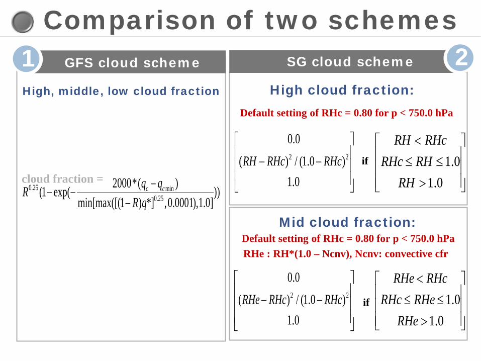
cloud fraction =
GFS cloud scheme 1 SG cloud scheme 2 High cloud fraction:
Mid cloud fraction:
2 2
0.0( ) / (1.0 )
1.0RH RHc RHc
− −
1.01.0
RH RHcRHc RH
RH
< ≤ ≤ >
2 2
0.0( ) / (1.0 )
1.0RHe RHc RHc
− −
1.01.0
RHe RHcRHc RHe
RHe
< ≤ ≤ >
RHe : RH*(1.0 – Ncnv), Ncnv: convective cfr Default setting of RHc = 0.80 for p < 750.0 hPa
High, middle, low cloud fraction
Default setting of RHc = 0.80 for p < 750.0 hPa
if
if
0.25 min0.25
2000*( )(1 exp( ))min[max([(1 ) *] ,0.0001),1.0]
c cq qRR q
−− −
−
Comparison of two schemes
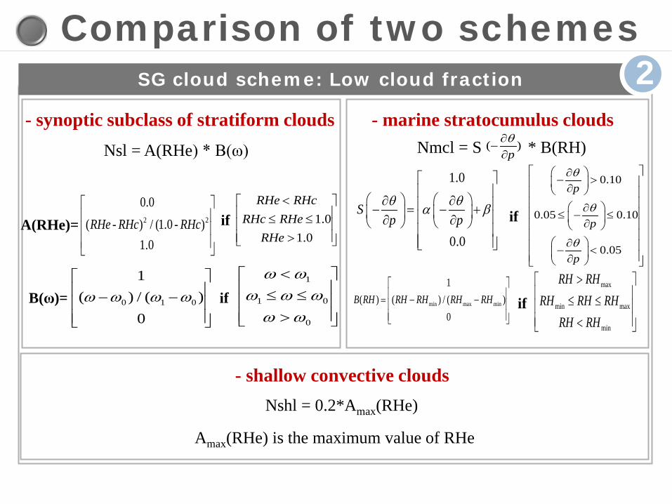
1 SG cloud scheme: Low cloud fraction 2
2 2
0.0( - ) / (1.0 - )
1.0RHe RHc RHc
1.01.0
RHe RHcRHc RHe
RHe
< ≤ ≤ >
0 1 0
1( ) / ( )
0ω ω ω ω
− −
1
1 0
0
ω ωω ω ωω ω
< ≤ ≤ >
- synoptic subclass of stratiform clouds Nsl = A(RHe) * B(ω)
A(RHe)=
B(ω)=
if
if
Nmcl = S * B(RH) ( )pθ∂
−∂
- marine stratocumulus clouds
1.0
0.0
Sp pθ θα β
∂ ∂ − = − + ∂ ∂
0.10
0.05 0.10
0.05
p
p
p
θ
θ
θ
∂− > ∂
∂ ≤ − ≤ ∂
∂ − < ∂
min max min
1( ) ( ) / ( )
0B RH RH RH RH RH
= − −
max
min max
min
RH RHRH RH RH
RH RH
> ≤ ≤ <
if
if
- shallow convective clouds Nshl = 0.2*Amax(RHe)
Amax(RHe) is the maximum value of RHe
Comparison of two schemes
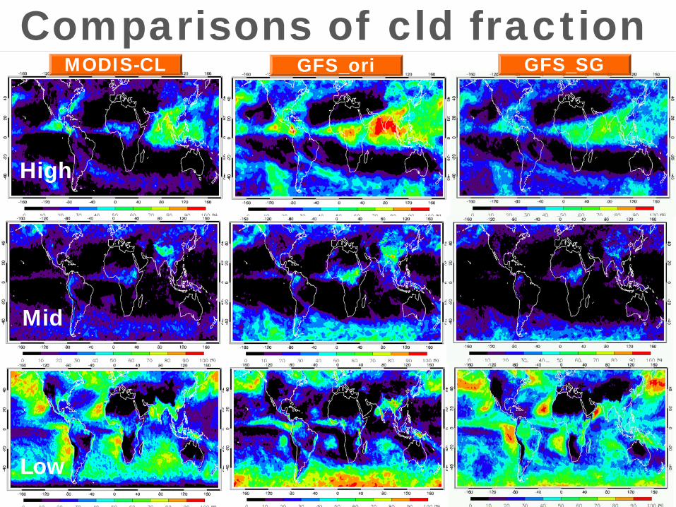
Comparisons of cld fraction MODIS-CL GFS_ori GFS_SG
High
Mid
Low
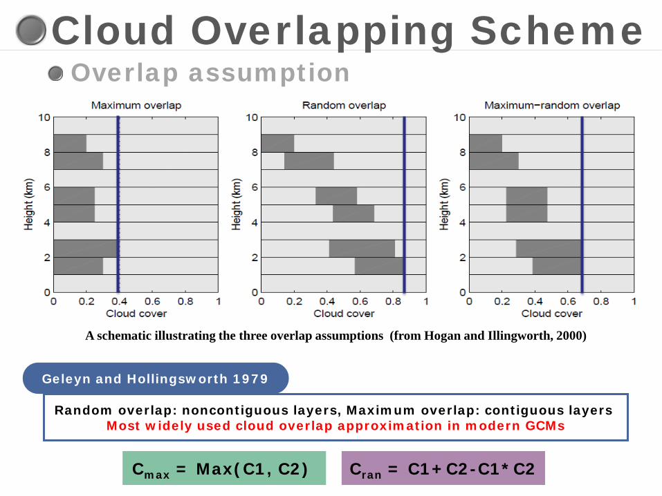
Overlap assumption
A schematic illustrating the three overlap assumptions (from Hogan and Illingworth, 2000)
Cmax = Max(C1, C2) Cran = C1+C2-C1*C2
Random overlap: noncontiguous layers, Maximum overlap: contiguous layers Most widely used cloud overlap approximation in modern GCMs
Geleyn and Hollingsworth 1979
Cloud Overlapping Scheme

Cloud Overlapping Scheme Previous studies Ctrue = a*Cmax + (1-a)*Cran ,where a(Δz) = exp(-Δz/Lcf)
▶ Mace and Benson-Troth
▶ For vertically continuous cloud, the degree of correlation between the cloud positions decreased with vertical separation of the layers Lcf : 4 km
E X P O N E N T I A L R A N D O M
▶ Pincus et al.
▶ Naud et al.
▶ Hogan and Illingworth
▶ Using CRM simulation, Stratiform and convective clouds have different overlap. St: Random, Con: Max
▶ Using MMCR Radar data from 4 ARM sites :SGP, TWP, Manus, Nauru Lcf : 3.9 km at SGP, 4 km at Manus, 4.6 km at Nauru
▶ Using cloud radar data from ARM with NCEP reanalysis data Lcf : 2 km at SGP, 2.3 km at Manus, 1.8 km at Nauru
▶ Barker
▶ Using CloudSat and CALIPSO data Lcf : median value of 2 km for global scales
▶ Shonk et al.
▶ Based on two studies, they suggest a simple linear fit Lcf : dependent on only latitudes
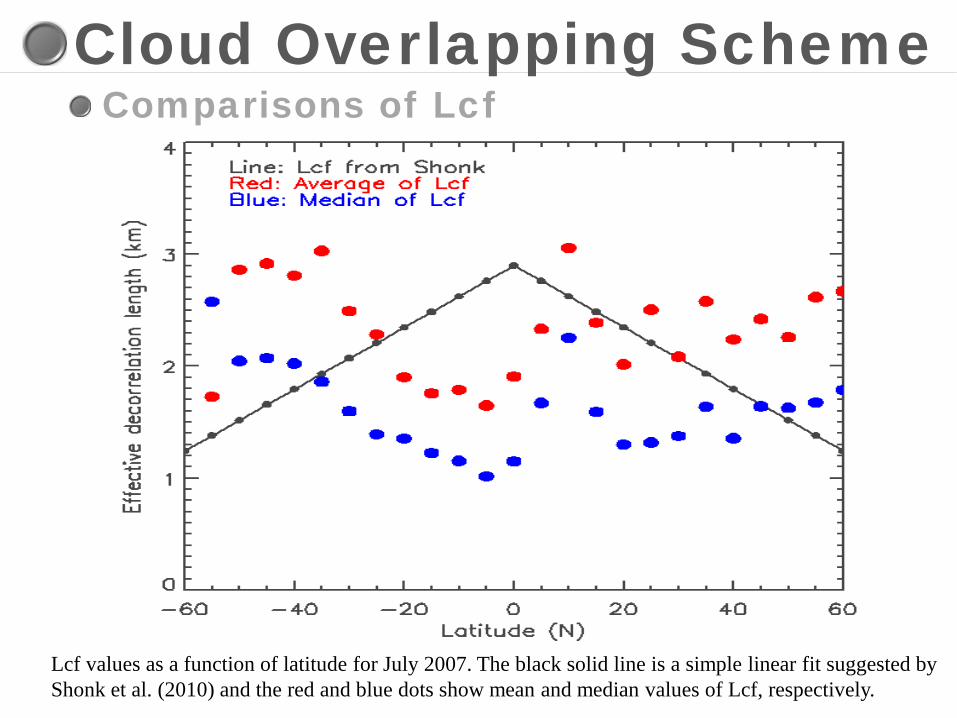
Comparisons of Lcf
Lcf values as a function of latitude for July 2007. The black solid line is a simple linear fit suggested by Shonk et al. (2010) and the red and blue dots show mean and median values of Lcf, respectively.
Cloud Overlapping Scheme

MODIS-CL GFS_ori GFS_Lcf
High
Mid
Low
Cloud Overlapping Scheme

Evaluation of GFS cloud properties
Change of cloud scheme
Change of cloud overlap assumption
Diagnosis input variables
Improvement
MODIS CERES AIRS CloudSat CALIPSO
ARM data

Publications Yoo, H., Z. Li, Y.-T. You, S.Lord, F. Weng, and H. W. Barker, 2013:Diagnosis and testing of low-level cloud parameterizations for the NCEP/GFS model satellite and ground-based measurements, Climate Dynamic, doi:10.1007/s00382-013-1884-8. Yoo, H., and Z. Li, (2012), Evaluation of cloud properties in the NOAA/NCEP Global Forecaster System using multiple satellite produt,
Climate Dynamics, 10.1007/s00382-012-1430-0. Zhang, J., Z. Li, H. Chen, M. Cribb, H. Yoo, 2013, Evaluation of Cloud Structure Simulated by NECP GFS using Ground-based Remote Sensing and Radiosonde Products at the ARM SGP site, Climate Dynamics, under revision.
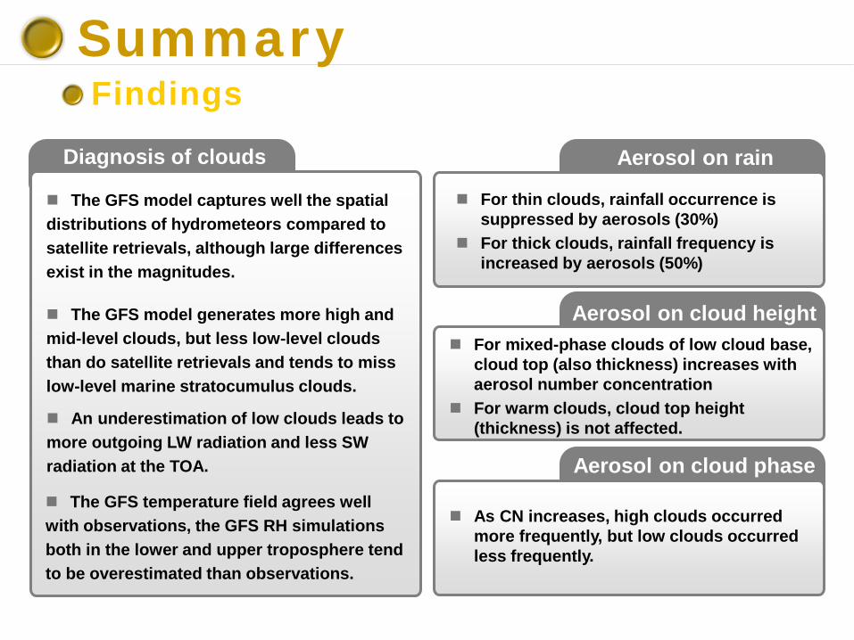
Summary Findings
Diagnosis of clouds Aerosol on rain
Aerosol on cloud height
Aerosol on cloud phase
As CN increases, high clouds occurred more frequently, but low clouds occurred less frequently.
For thin clouds, rainfall occurrence is suppressed by aerosols (30%)
For thick clouds, rainfall frequency is increased by aerosols (50%)
For mixed-phase clouds of low cloud base, cloud top (also thickness) increases with aerosol number concentration
For warm clouds, cloud top height (thickness) is not affected.
The GFS model captures well the spatial distributions of hydrometeors compared to satellite retrievals, although large differences exist in the magnitudes. The GFS model generates more high and mid-level clouds, but less low-level clouds than do satellite retrievals and tends to miss low-level marine stratocumulus clouds.
An underestimation of low clouds leads to more outgoing LW radiation and less SW radiation at the TOA.
The GFS temperature field agrees well with observations, the GFS RH simulations both in the lower and upper troposphere tend to be overestimated than observations.

Diagnosis
Joint histograms of CTP and COD derived from retrievals by applying the C-L algorithm (left), the MODIS-EOS products (middle), and the GFS model (right) in July 2007.
MODIS-CL MODIS-EOS GFS
Cloud top pressure and cloud optical depth

Diagnosis Multi-layered cloud occurrence
0
20
40
60
80
100
-60 -40 -20 0 20 40 60
Single C-CSingle GFSDual C-CDual GFS
Latitude (0N)
0
20
40
60
80
100
-60 -40 -20 0 20 40 60
Single C-CSingle GFSDual C-CDual GFS
Latitude (0N)
Latitudinal variations of the frequencies of cloud occurrence from the C-C satellites and the GFS model for single and dual-layer clouds in January (left) and July (right) of 2007.
January July
Data & approach
T
RH
CF Height COD
T
LW
SW
RH CF
CloudSat CALIPSO
CERES
ARM SGP site
Observation
AIRS COD
IWP
LWP
CF
MODIS
from NASA site
Satellites