event study a change point approach slides

IntroductionThe Change-Point Model

Empirical AnalysisSummary

References

Event Study: A Change-Point Model Approach

JOON-HUI YOON

Department of Industrial and Systems EngineeringUniversity of [email protected]

Joint work with Farid AitSahlia

April 23, 2009

1 / 29



References

Introduction

Event study:A statistical method to assess the impact of events on the value of a firm

Change-point model approach:Bayesian method to determine latent variables (regime levels) and the timesat which they change on the basis of related observations (e.g., asset prices)

2 / 29



References

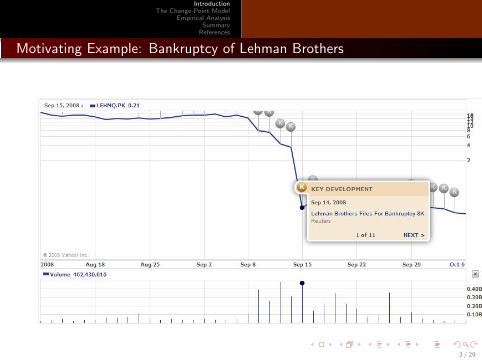
Motivating Example: Bankruptcy of Lehman Brothers

3 / 29



References

Fundamental Definitions

Direction: expected value of rate of return of equity price over time

Volatility: standard deviation of rate of return of equity price over time

Structural break: a significant departure in direction and volatility fromthe immediate past

Regime: a distinguishable set consisting of a time interval, a directionvalue and a volatility value

4 / 29



References

Fundamental Problems

What is the market price discovery process in relation to an event?

If some traders know the information earlier than when it is announced,can we detect it?

How can we estimate directions and volatilities in the regime?

How do we detect structural breaks around key developments (events)?

Are there any properties common to disparate key developments?

5 / 29



References

Objectives of the Proposed Study

Propose a change-point model to detect structural breaks in an eventwindow

Show empirical evidence of structural breaks

Discuss implications between the breaks and key developments, especiallythe ex-ante/ex-post contrast

6 / 29



References

Key Findings

Price adjustments to key developments may begin before and end after theannouncement

Statistical correlation between successive key developments is notsignificant

7 / 29



References

Methodology: Overview

Parametrization

Gibbs sampling

Markov chain expectation-maximization (MCEM)

Bayes factor

8 / 29



References

Parametrization: Abnormal Return

Abnormal return at at time t is defined by,

at := rt −[α + βrm

t + sSMBt + hHMLt

](1)

Regime st in a regime set ST = {st}, {t = 1, . . . , T} follows discrete-stateMarkov chain where pij = P(st = j |s(t−1) = i) with transition diagram,

at follows IID Normal with mean µs and variance σ2s given the regime of

time t is s,

at |st = s ∼ N (µs , σ2s ), t = 1, 2, . . . , T , s = 1, 2, . . . , S (2)

Prior densities of parameter π(µs , σ2s ) = π(µs |σ2

s )π(σ2s ) and regime set

distribution π(pss) follow Normal, Inverse Gamma, and Beta respectively,

σ2s ∼ IG

(ν0

2,σ2

0

2

), µs |σ2

s ∼ N(

µ0,σ2

s

κ0

), pss ∼ B(a0, b0) (3)

9 / 29



References

Gibbs sampling: Estimating Structural Break Points(Continued)

After M iterations of Gibbs sampler, we find marginal posterior of regimeset,

π(st = k|AT ) :=

∫π(st = k|At−1, Θ, P)π(Θ, P|AT )d(Θ, P) (7)

≈ 1

M

M∑m=1

π(s(m)t = k|A(m)

t−1, Θ(m), P(m)) (8)

11 / 29



References

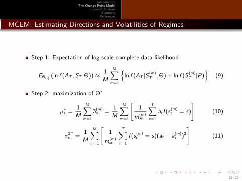
MCEM: Estimating Directions and Volatilities of Regimes

Step 1: Expectation of log-scale complete data likelihood

EΘ(i)(ln f (AT , ST |Θ)) ≈ 1

M

M∑m=1

{ln f (AT |S (m)

T , Θ) + ln f (S(m)T |P)

}(9)

Step 2: maximization of Θ∗

µ∗s =1

M

M∑m=1

a(m)s =

1

M

M∑m=1

[1

m(m)ss

T∑t=1

at I (s(m)t = s)

](10)

σ2s∗

=1

M

M∑m=1

[1

m(m)ss

T∑t=1

I (s(m)t = s)(at − a(m)

s )2

](11)

12 / 29



References

Partial R code

#Gibbs samp l i ng : ma rg i na l p o s t e r i o r o fSn

k <− 1 #r e p e t i t i o n i ndexr e p e a t{MCMCpart1 (1 , k ) #Gene r a t i ng PMCMCpart2 (1 , k ) #Gene r a t i ng Theta (muK or

sigmaKsq )MCMCpart3 (1 , k ) #Gene r a t i ng Sn , N i ii f ( k>=nsimMCMC+t r a n s i e n t ){ #te rm i n a t i n g

c o n d i t i o ntermMCMC <− 0break}

r e po r tRe co rd ( i f ( r e p o r t F l a g [2]==TRUE){2}e l s e {0})

k <− k+1i f ( k> t r a n s i e n t ){#Sto r i n g Sn and N i i to

be used i n c a l c u l a t i n g ma rg i na ll i k e l i h o o d

SnM[ k−t r a n s i e n t , ] <− SnNiiM [ k−t r a n s i e n t , ] <− N i i}

}MCMCTrials <− k#marg i na l p o s t e r i o r o f s t a t e s SnmarPostSnProb <− sumPsYtm1TP/nsimMCMCr epo r tE xpo r t ( i f ( r e p o r t F l a g [2]==TRUE){2}

e l s e {0})

#MCEM: Marg ina l l i k e l i h o o dr e p e a t{MCMCpart1 (2 , k ) #Gene r a t i ng MLE o f PMCMCpart2 (2 , k ) #Gene r a t i ng MLE o f Theta (

muK, sigmaKsq )i f ( k<=nsimMCEM/3){N <− Ncand [ 1 ] #

r e i n i t i a l i z e N, i n c r e a s i n g as ki n c r e a s e s

} e l s e i f ( k<=2∗nsimMCEM/3){N <− Ncand [ 2 ]} e l s e{N <− Ncand [ 3 ]}Sn <− mat r i x (NA, nrow = N, nco l=l e ng t h (

Yn) )N i i <− mat r i x (NA, nrow = N, nco l=M[ j ] )MCMCpart3 (2 , k ) #Part 3 : Gene r a t i ng Sn ,

N i ii f ( k>=nsimMCEM){ #te rm i n a t i n g c o n d i t i o n

termMCEM <− 1break}

r e po r tRe co rd ( i f ( r e p o r t F l a g [3]==TRUE){3}e l s e {0})

k <− k+1}MCEMTrials <− kMLEsigmaKsq <− sigmaKsq ; MLEmuK <− muK;

MLETrnPrb <− TrnPrb #MLEsMLESn <− Sn ; MLENii <− N i i ; MLEN <− N

14 / 29



References

Partial R code(Continued)

#Marg ina l l i k e l i h o o d MLEPsYtm1TP <− MCMCpart3 (3 , k )y t L i k e A l l <− mat r i x (NA, nrow = l e ng t h (Yn) , n co l = M[ j ] )sumPiTYS <− 0 ; sumPiPYT <− 0s igmaKsqLikePr=muKLikePr<−r ep (NA, t imes=M[ j ] ) n i i L i k e P r <−r ep (NA, t imes=M[ j ]−1) f o r ( l i n 1 :M[ j ] ){

y t L i k e A l l [ , l ] <− dnorm (Yn ,MLEmuK[ l ] , s q r t (MLEsigmaKsq [ l ] ) )}f o r (m i n 1 :nsimMCMC){

Sn <− SnM[m, ] ; N i i <<− NiiM [m, ] sumPiTYS <− sumPiTYS + MCMCpart2 (3 , k )}i f (M[ j ]==1){

sumPiPYT <− nsimMCMC} e l s e{ f o r (m i n 1 :MLEN){

N i i <<− MLENii [m, ]f o r ( l i n 1 : (M[ j ]−1) ){

n i i L i k e P r [ l ] <− dbeta (MLETrnPrb [ l ] , a0+N i i [ l ] , b0+1)}sumPiPYT <− sumPiPYT + prod ( n i i L i k e P r )}}

f o r ( l i n 1 :M[ j ] ){s igmaKsqLikePr [ l ] <− dinvgamma (MLEsigmaKsq [ l ] , nu0 /2 ,s igma0sq /2) #p o s t e r i o r MLE sigmaKsq l i k e l i h o o d on p r i o rmuKLikePr [ l ] <− dnorm (MLEmuK[ l ] , mu0 ,s q r t (MLEsigmaKsq [ l ] / kappa0 ) )} #p o s t e r i o r MLE mu l i k e l i h o o d on p r i o r

margLike <− sum( l o g ( rowSums ( y t L i k e A l l ∗MLEPsYtm1TP) ) ) +l og ( prod ( s igmaKsqL ikePr ) ) + l og ( prod ( muKLikePr ) ) −l o g ( sumPiTYS/nsimMCMC) − l o g ( sumPiPYT/nsimMCMC)

15 / 29



References

Empirical Analysis: Data Specification

Firm selection: Russell 3000, COMPUSTAT

Key Development: Reuters Knowledge

Abnormal Return: EVENTUS@WRDS

Software: R and MySQL

16 / 29



References

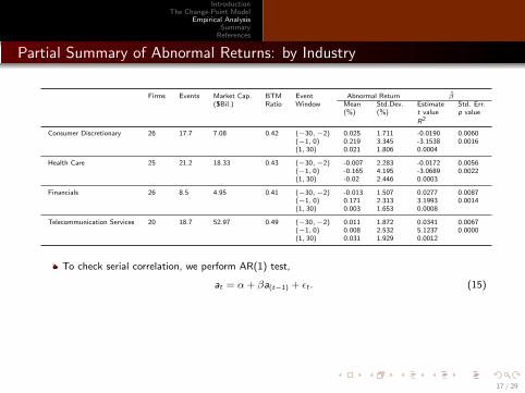
Partial Summary of Abnormal Returns: by Industry

Firms Events Market Cap. BTM Event Abnormal Return β($Bil.) Ratio Window Mean Std.Dev. Estimate Std. Err.

(%) (%) t value p value

R2

Consumer Discretionary 26 17.7 7.08 0.42 (−30,−2) 0.025 1.711 -0.0190 0.0060(−1, 0) 0.219 3.345 -3.1538 0.0016(1, 30) 0.021 1.806 0.0004

Health Care 25 21.2 18.33 0.43 (−30,−2) -0.007 2.283 -0.0172 0.0056(−1, 0) -0.165 4.195 -3.0689 0.0022(1, 30) -0.02 2.446 0.0003

Financials 26 8.5 4.95 0.41 (−30,−2) -0.013 1.507 0.0277 0.0087(−1, 0) 0.171 2.313 3.1993 0.0014(1, 30) 0.003 1.653 0.0008

Telecommunication Services 20 18.7 52.97 0.49 (−30,−2) 0.011 1.872 0.0341 0.0067(−1, 0) 0.008 2.532 5.1237 0.0000(1, 30) 0.031 1.929 0.0012

To check serial correlation, we perform AR(1) test,

at = α + βa(t−1) + εt . (15)

17 / 29



References

Summary of Abnormal Returns: by Market Cap. and BTM

Firms Events Market Cap. BTM Event Abnormal Return β($Bil.) Ratio Window Mean Std.Dev. Estimate Std. Err.

(%) (%) t value p value

R2

Big 136 19.4 23.03 0.44 (−30,−2) 0.004 1.784 -0.0134 0.0025(−1, 0) 0.016 3.059 -5.3353 0.0000(1, 30) 0.002 1.884 0.0002

Small 101 9.8 1.08 0.45 (−30,−2) 0.003 2.23 -0.0184 0.0041(−1, 0) 0.161 3.889 -4.4889 0.0000(1, 30) 0.02 2.334 0.0003

Value 82 14.9 7.94 0.71 (−30,−2) 0.006 1.8 -0.0322 0.0037(−1, 0) -0.042 3.304 -8.7514 0.0000(1, 30) -0.012 1.929 0.0010

Mid 83 16.4 26.71 0.4 (−30,−2) 0.001 1.736 -0.0249 0.0035(−1, 0) 0.13 3.025 -7.1085 0.0000(1, 30) 0.026 1.782 0.0006

Growth 72 14.6 15.17 0.19 (−30,−2) 0.005 2.24 0.0054 0.0040(−1, 0) 0.072 3.637 1.3707 0.1705(1, 30) 0.003 2.371 0.0000

18 / 29



References

Announcement of Key Developments: Characteristics

β KPSS KS-E KS-NKey Development Estimate Std. Err. t value KPSS level D stat. D stat.

Arrivals p value R2 p value p value p value

Big 2713 0.25 0.02 14.38 0.17 0.05 0.170 0.07 0.1 0 0.00

Small 981 0.17 0.03 5.86 0.12 0.09 0.180 0.03 0.1 0 0.00

Value 1290 0.26 0.03 10.49 0.82 0.05 0.180 0.08 0.01 0 0.00

Mid 1347 0.23 0.03 8.67 0.78 0.06 0.190 0.05 0.01 0 0.00

Growth 1057 0.24 0.03 9.03 0.52 0.06 0.170 0.07 0.04 0 0.00

19 / 29



References

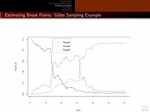
Estimating Break Points: Gibbs Sampling Example

20 / 29



References

Estimating Direction and Volatility: MCEM Example

21 / 29



References

Selecting the Best Change-Point Model: Bayes Factor Example

Compared Model Upper Confidence Limit p valueTicker Model M1 M2 M3 M4 M1 M2 M3 M4 M1 M2 M3 M4AA 1 0.00 -0.28 16.78 -3.94 NA 2.15 58.06 1.92 0.00 0.06 0.73 0.05

2 0.28 0.00 17.06 -3.66 2.71 NA 58.32 2.16 0.12 0.00 0.73 0.053 -16.78 -17.06 0.00 -20.72 24.50 24.19 NA 19.54 0.22 0.22 0.00 0.174 3.94 3.66 20.72 0.00 9.81 9.48 60.98 NA 0.71 0.68 0.78 0.00

JCP 1 0.00 30.63 28.71 12.44 NA 67.59 57.22 30.92 0.00 0.90 0.94 0.832 -30.63 0.00 -1.92 -18.19 6.32 NA 33.23 23.93 0.07 0.00 0.43 0.213 -28.71 1.92 0.00 -16.27 -0.21 37.07 NA 11.13 0.04 0.50 0.00 0.134 -12.44 18.19 16.27 0.00 6.03 60.31 43.68 NA 0.10 0.74 0.81 0.00

All Firms 1 0.0000 12.7231 13.5696 29.5629 NA 17.5675 18.8539 36.8193 0.0000 0.9999 0.9998 1.00002 -12.7231 0.0000 0.8466 16.8398 -7.8786 NA 6.4587 25.0420 0.0000 0.0000 0.3676 0.99853 -13.5696 -0.8466 0.0000 15.9933 -8.2853 4.7655 NA 24.3442 0.0000 0.2019 0.0000 0.99704 -29.5629 -16.8398 -15.9933 0.0000 -22.3065 -8.6377 -7.6423 NA 0.0000 0.0001 0.0002 0.0000

22 / 29



References

Selecting the Best Change-Point Model(Continued)

Ticker Mr Ticker Mr Ticker Mr Ticker Mr

AA 4 FDX 3 PDX 1 TMO 4AEP 1 FL 1 PG 1 TSN 1BIIB 3 GCO 1 PLCE 1 UNH 2BSX 3 JCP 1 PTRY 4 VZ 3CAT 3 KFT 2 QCOM 1 WYE 2CELG 4 MGM 1 S 1EGN 1 MON 1 T 1

23 / 29



References

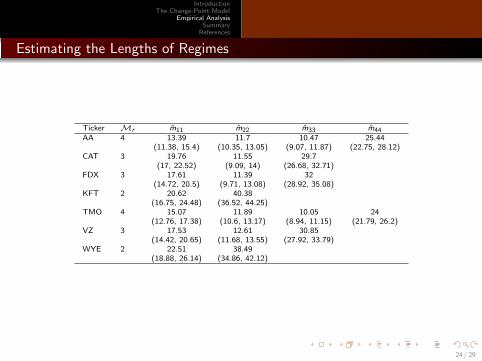
Estimating the Lengths of Regimes

Ticker Mr m11 m22 m33 m44AA 4 13.39 11.7 10.47 25.44

(11.38, 15.4) (10.35, 13.05) (9.07, 11.87) (22.75, 28.12)CAT 3 19.76 11.55 29.7

(17, 22.52) (9.09, 14) (26.68, 32.71)FDX 3 17.61 11.39 32

(14.72, 20.5) (9.71, 13.08) (28.92, 35.08)KFT 2 20.62 40.38

(16.75, 24.48) (36.52, 44.25)TMO 4 15.07 11.89 10.05 24

(12.76, 17.38) (10.6, 13.17) (8.94, 11.15) (21.79, 26.2)VZ 3 17.53 12.61 30.85

(14.42, 20.65) (11.68, 13.55) (27.92, 33.79)WYE 2 22.51 38.49

(18.88, 26.14) (34.86, 42.12)

24 / 29



References

Direction and Volatility Differences in Consecutive Regimes

Welch Two Sample t test(Confidence Limit)(p value)

Ticker Mr µ1 µ2 µ3 µ4 µ1 − µ2 µ2 − µ3 µ3 − µ4AA 4 0.0017 -0.002 -0.0031 -0.0002 (-0.0037, 0.011) (0.3205) (-0.0093, 0.0116) (0.8257) (-0.0115, 0.0056) (0.4839)CAT 3 -0.0016 -0.0053 0.0008 (-0.0049, 0.0123) (0.393) (-0.0143, 0.0021) (0.1411)FDX 3 -0.0012 0.0011 -0.0009 (-0.006, 0.0014) (0.2173) (-0.0015, 0.0055) (0.265)KFT 2 0.0018 0.0003 (-0.0033, 0.0063) (0.5324)TMO 4 0.001 -0.0072 0.0049 0.0007 (-0.0021, 0.0185) (0.1153) (-0.0231, -0.001) (0.0328) (-0.0011, 0.0094) (0.1191)VZ 3 -0.0012 0.0027 0.0006 (-0.0068, -0.0009) (0.0115) (-0.001, 0.005) (0.1827)WYE 2 0.0003 -0.0003 (-0.0014, 0.0025) (0.5856)

σ1 σ2 σ3 σ4 σ1 − σ2 σ2 − σ3 σ3 − σ4AA 4 0.0079 0.0085 0.0088 0.0103 (-0.0042, 0.0031) (0.7646) (-0.0039, 0.0033) (0.8652) (-0.004, 0.0009) (0.2038)CAT 3 0.0098 0.0081 0.0097 (-0.002, 0.0053) (0.3621) (-0.0044, 0.0012) (0.26)FDX 3 0.0085 0.0083 0.0093 (-0.0029, 0.0033) (0.919) (-0.004, 0.002) (0.5155)KFT 2 0.006 0.009 (-0.0049, -0.0011) (0.0022)TMO 4 0.0062 0.0081 0.0073 0.0082 (-0.0049, 0.0011) (0.2179) (-0.0023, 0.0039) (0.6138) (-0.0034, 0.0016) (0.47)VZ 3 0.0059 0.006 0.0065 (-0.0021, 0.0018) (0.8924) (-0.0023, 0.0014) (0.6252)WYE 2 0.0074 0.011 (-0.0059, -0.0013) (0.0023)

25 / 29



References

Correlation and Serial Correlation of Directions and Volatilities

µj = β0 + β1µi + β2σi + β3σj

σj = β0 + β1µi + β2σi + β3µj p values

Ticker Mr (i, j) µ/σ β0 β1 β2 β3 β0 β1 β2 β3 R2

AA 4 (1, 2) µ 0 -0.2445 -0.3351 0.1231 0.9975 0.5407 0.6096 0.7836 0.0227σ 0.0054 -0.0311 0.3938 0.024 0.0549 0.8607 0.1672 0.7836 0.0799

(2, 3) µ -0.0169 -0.0626 0.1476 1.4073 0.0613 0.7873 0.7733 0.0802 0.1237σ 0.0086 -0.0073 0.0505 0.0804 0 0.8949 0.6801 0.0802 0.1249

(3, 4) µ -0.0002 -0.0139 0.0395 -0.0306 0.9455 0.8044 0.864 0.9155 0.0028σ 0.0097 -0.0376 0.0629 -0.0144 0 0.3239 0.6907 0.9155 0.0377

KFT 2 (1, 2) µ -0.0045 0.0195 0.014 0.5252 0.0001 0.3716 0.8333 0 0.5771σ 0.0091 -0.0364 -0.061 1.0931 0 0.2451 0.5223 0 0.5903

VZ 3 (1, 2) µ 0.0069 -0.0979 -0.2916 -0.4444 0.0313 0.7648 0.4326 0.196 0.1065σ 0.0057 0.0377 0.1338 -0.1427 0.001 0.839 0.526 0.196 0.0964

(2, 3) µ -0.0008 -0.0344 0.0681 0.1675 0.7743 0.7901 0.7721 0.5482 0.0171σ 0.0076 0.0611 -0.2121 0.0838 0 0.5026 0.195 0.5482 0.1109

WYE 2 (1, 2) µ -0.0041 -0.0468 0.0712 0.3016 0.0143 0.6724 0.5335 0.0114 0.2363σ 0.0117 -0.0248 -0.0662 0.7357 0 0.8861 0.7114 0.0114 0.2273

Linear autoregressive panel data models are used,

µj = β10 + β1

1 µi + β12 σi + β1

3 σj + ε1j , (16)

σj = β20 + β2

1 µi + β22 σi + β2

3 µj + ε2j , (17)

where i = 1, . . . , S − 1, j = 2, . . . , S

26 / 29



References

Summary

Estimated variable lengths of multiple regimes using Gibbs sampler

Estimated directions and volatilities of abnormal returns by MCEM

Evaluated models with various number of regimes

Best model defined as having highest Bayes factor

Not all key developments produce structural breaks

Breakpoints may not necessarily coincide with announcement date

Serial correlation between successive directions/volatilities are notstatistically significant

27 / 29



References

Further Study

Extend the analysis to liquidity changes in intraday data by accounting for

adverse selection component in bid-ask spreads as in [Itzhak and Lee, 1996]

regime changes in realized volatility as in [Liu and Maheu, 2008]

28 / 29



References

References

Siddhartha Chib. Estimation and comparison of multiple change-point models.Journal of Econometrics, 86(2):221 - 241, 1998.

Pastor, Lubos and Stambaugh, Robert F. The Equity Premium and StructuralBreaks. The Journal of Finance, 56(4):1207–1239, Aug., 2001.

Liu, Chun and Maheu, John M. Are There Structural Breaks in RealizedVolatility? Journal of Financial Econometrics, Vol. 6, Issue 3, pp.326-360, 2008.

Krinsky, Itzhak and Jason Lee. Earnings Announcements and the Componentsof the Bid-Ask Spread. The Journal of Finance, Vol. 51, Issue 4, pp.1523–1535, Sep., 1996.

29 / 29

event study a change point approach slides

Documents