Evolution Strategies with Cumulative Step Length Adaptation on

the Noisy Parabolic Ridge

Dirk V. Arnold

Hans-Georg Beyer

Technical Report CS-2006-02

January 16, 2006

Faculty of Computer Science6050 University Ave., Halifax, Nova Scotia, B3H 1W5, Canada

Evolution Strategies with Cumulative Step Length

Adaptation on the Noisy Parabolic Ridge

Dirk V. ArnoldFaculty of Computer Science, Dalhousie University, Halifax, Nova Scotia,

Canada B3H 1W5

Hans-Georg BeyerDepartment of Computer Science, Research Center Process and Product

Engineering, Vorarlberg University of Applied Sciences, Hochschulstr. 1, A-6850

Dornbirn, Austria

Abstract. This paper presents an analysis of the performance of the (µ/µ, λ)-ES with isotropic mutations and cumulative step length adaptation on the noisyparabolic ridge. Several forms of dependency of the noise strength on the distancefrom the ridge axis are considered. Closed form expressions are derived that describethe mutation strength and the progress rate of the strategy in high-dimensionalsearch spaces. It is seen that as for the sphere model, larger levels of noise present leadto cumulative step length adaptation generating increasingly inadequate mutationstrengths, and that the problem can be ameliorated to some degree by working withlarger populations.

Keywords: Evolutionary computation, evolution strategies, optimisation, noise,cumulative step length adaptation, ridge functions

1. Introduction

Evolution strategies are a type of evolutionary algorithm that is mostcommonly used for the optimisation of real-valued functions of the formf : IRN → IR. Typical features of evolution strategies include the useof truncation selection, normally distributed mutations, and some formof self-adaptation for step length control. See [13] for a comprehensiveintroduction. Much work has gone into the analysis of the behaviour ofevolution strategies on simple objective functions, such as the spheremodel [1, 5, 11, 23], ellipsoidal fitness landscapes [12], the corridormodel [22], and the ridge function class [10, 20, 21, 19, 23]. Whilethe sphere and the ellipsoids serve as models for fitness landscapes inthe vicinity of local optima, both the corridor and the ridge strive tomodel features of such landscapes in greater distance from the optima.More specifically, they test the ability of a strategy to make progressin a particular direction in search space, where deviation from thatdirection is penalised. The goal of such analyses is to derive scalinglaws that help reveal strengths and weaknesses of particular strategy

main.tex; 16/01/2006; 14:04; p.1

2

variants, to make recommendations with regard to the setting of thestrategies’ exogenous parameters, and to contribute to the continuedimprovement of existing and the design of new strategy variants.

Ridge functions are known to pose significant problems for optimi-sation strategies. Whitley, Lunacek, and Knight [26] point out thatwhile the difficulties of optimising ridges “are relatively well docu-mented in the mathematical literature on derivative free minimizationalgorithms [. . . ], there is little discussion of this problem in the heuris-tic search literature”. For evolutionary algorithms in particular, whilelong term progress is best achieved with large step lengths, mutationstrength adaptation mechanisms are often shortsighted and generatestep lengths much shorter than optimal. This deficiency on ridges isthe cause of the premature convergence of evolution strategies on aunimodal objective function that has been observed by Salomon [25].

Several steps have been made toward a quantitative understandingof the behaviour of evolution strategies on ridge functions. Rechen-berg [23] provides (without derivation) a formula for the progress rateof evolution strategies on the parabolic ridge. However, that formulacontains the location in search space as a parameter, and no attemptis made to model the distribution of the population in search space.Oyman, Beyer and Schwefel [20, 21] study the performance of the(1 +, λ)-ES with fixed mutation strength on the parabolic ridge andderive formulas both for the average distance from the ridge axis and forthe progress rate of the algorithm. They find that the comma strategy isgenerally superior to the plus strategy. In a generalisation of that work,Oyman and Beyer [19] study the behaviour of the (µ/µ, λ)-ES with bothintermediate and dominant recombination. Beyer [10] also considers theperformance of the (1, λ)-ES on ridges other than the parabolic one andfinds that qualitatively different behaviours can result on different ridgetopologies. Insights with regard to the issue of step length adaptationthat have been published so far are purely empirical and include theaforementioned paper by Salomon [25] as well as results provided byHerdy [17].

This paper studies the performance of evolution strategies with in-termediate multirecombination and cumulative step length adaptationon the noisy parabolic ridge function class. It thus extends previouswork [19, 21] in two directions: first, it considers the influence of noise;and second, it analytically studies the performance of cumulative steplength adaptation. Its remainder is organised as follows. Section 2describes the (µ/µ, λ)-ES with cumulative step length adaptation, sum-marises some results on expected values of order statistics that areused later in the paper, and briefly reviews the approach to the anal-ysis of the sphere model that will be seen to form an important step

main.tex; 16/01/2006; 14:04; p.2

3

in the investigation of the ridge function class. Section 3 studies theperformance of the (µ/µ, λ)-ES on the noisy parabolic ridge withoutconsidering step length adaptation. Scaling laws for the progress rateas well as for the average distance from the ridge axis are derived, andseveral forms of dependency of the noise strength on the distance fromthe ridge axis are considered. The results are obtained in the limit ofinfinite search space dimensionality and their significance is verifiedin experiments in finite-dimensional search spaces. Section 4 includescumulative step length adaptation in the analysis. Section 5 concludeswith a brief summary of the results and suggestions for future research.

2. Preliminaries

This section first describes the (µ/µ, λ)-ES with isotropic mutationsand cumulative step length adaptation for the optimisation of functionsf : IRN → IR. Next, terminology and two useful lemmas from the fieldof order statistics are introduced. Then, some important results withregard to the behaviour of the (µ/µ, λ)-ES on the quadratic spheremodel are summarised. Those results form a cornerstone in the analysisof the behaviour of the (µ/µ, λ)-ES on the ridge function class presentedin Sections 3 and 4.

2.1. The (µ/µ, λ)-ES

The strategy under consideration in this paper is the (µ/µ, λ)-ES withisotropic mutations and intermediate recombination. That strategy ispopular due to both its good performance and its amenability to math-ematical analysis. The following description of the algorithm is delib-erately brief. See [13] for a more comprehensive discussion of evolutionstrategies and their naming conventions, and see [18] for a thoroughmotivation of cumulative step length adaptation.

In every time step the (µ/µ, λ)-ES computes the centroid of thepopulation of candidate solutions as a search point x ∈ IRN thatmutations are applied to. For the purpose of adapting the mutationstrength, a vector s ∈ IRN that is referred to as the search path is usedto accumulate information about the directions of the most recentlytaken steps. An iteration of the strategy updates the search point alongwith the search path and the mutation strength of the strategy in fivesteps:

1. Generate λ offspring candidate solutions y(i) = x + σz(i), i =1, . . . , λ, where mutation strength σ > 0 determines the step length

main.tex; 16/01/2006; 14:04; p.3

4

and the z(i) are vectors consisting of N independent, standardnormally distributed components.

2. Determine the objective function values f(y(i)) of the offspringcandidate solutions and compute the average

z(avg) =1

µ

µ∑

k=1

z(k;λ) (1)

of the µ best of the z(i). The index k;λ refers to the kth best ofthe λ offspring candidate solutions (i.e., the kth largest if the taskis maximisation and the kth smallest if the task is minimisation).Vector z(avg) is referred to as the progress vector.

3. Update the search point according to

x← x + σz(avg). (2)

Clearly, the new search point is the arithmetic mean of the µ bestof the offspring candidate solutions.

4. Update the search path according to

s← (1− c)s +√

µc(2− c)z(avg), (3)

where the cumulation parameter c determines how rapidly the di-rection information stored in s fades.

5. Update the mutation strength according to

σ ← σ exp

(

‖s‖2 −N

2DN

)

, (4)

where D serves as a damping factor in the adaptation process.

Following recommendations given by Hansen [15], the cumulation pa-rameter c and damping constant D are set to 1/

√N and

√N , respec-

tively. It is the goal of cumulative step length adaptation to adaptthe mutation strength such that correlations between successive stepsare eliminated. The coefficients in Eq. (3) are chosen such that thesearch path s consists of standard normally distributed components ifselection is random. The strategy used here differs from the original onedescribed in [18] in that in Eq. (4), adaptation is accomplished basedon the squared length of the search path rather than on its length. Thismodification will simplify the analysis in Section 4 without significantlyimpacting the algorithm’s performance.

main.tex; 16/01/2006; 14:04; p.4

5

2.2. Some Results on Expected Values of Order Statistics

Let X1, X2, . . . , Xλ be a random sample from some univariate prob-ability distribution, and arrange the Xi in nondecreasing order suchthat X1:λ ≤ X2:λ ≤ · · · ≤ Xλ:λ. The kth smallest of the Xi is denotedby Xk:λ and referred to as the kth order statistic of the sample. SeeBalakrishnan and Rao [7] for an introduction to the area of orderstatistics. The following lemma gives an expression for the expectedvalue of the mean of the µ largest of the Xi for the case that thesample members are independently drawn from a normal distribution.

LEMMA 1. Let X1, X2, . . . , Xλ be λ independent, standard normallydistributed random variables. Then the expected value of the arithmeticmean of the (λ + 1− µ)th through λth order statistics is

E

[

1

µ

µ∑

k=1

Xλ+1−k:λ

]

= cµ/µ,λ (5)

where

cµ/µ,λ =λ− µ

2π

(

λ

µ

)

∫

∞

−∞

e−x2

[Φ(x)]λ−µ−1[1− Φ(x)]µ−1dx

is the (µ/µ, λ)-progress coefficient defined in [11] and where Φ(x) de-notes the cumulative distribution function of the standardised normaldistribution.

See [11] for a derivation of this result. Figure 1 illustrates how the(µ/µ, λ)-progress coefficient depends on the population size parame-ters µ and λ. Lemma 1 will be seen to be useful when there is a directconnection between a random variable characterising a component ofa mutation vector and the fitness of the corresponding offspring candi-date solution. However, both in the presence of noise and on the ridgefunction class, that connection is only indirect, and a generalisation ofthe lemma is required.

Let (X1, Y1), (X2, Y2), . . . , (Xλ, Yλ) be a random sample from somebivariate probability distribution. If the sample is ordered by the Xi,then the Y -variate associated with the kth order statistic Xk:λ is de-noted by Y[k:λ] and referred to as the concomitant of the kth orderstatistic. See David and Nagaraja [14] for a treatment of concomitantsof order statistics. The following lemma gives an expression for theexpected value of the arithmetic mean of the concomitants of the µlargest order statistics for the case that X = Y +Z, where both Y andZ are normally distributed.

main.tex; 16/01/2006; 14:04; p.5

6

0.0

1.0

2.0

3.0

0.0 0.2 0.4 0.6 0.8 1.0

PSfrag replacements

truncation ratio µ/λ

pro

gres

sco

effici

ent

c µ/µ,λ

Figure 1. Progress coefficients cµ/µ,λ plotted against the ratio µ/λ for differentvalues of λ. The curves correspond to, from bottom to top, λ = 4, 10, 40, 100,and the limit case λ = ∞. The curves are displayed in the range from 1/λ to 1. Notethat only values µ/λ with integer µ are of interest.

LEMMA 2. Let Y1, Y2, . . . , Yλ be λ independent, standard normallydistributed random variables, and let Z1, Z2, . . . , Zλ be λ independent,normally distributed random variables with mean zero and with vari-ance ϑ2. Then, defining Xi = Yi + Zi for i = 1, . . . , λ and orderingthe sample members by nondecreasing values of the X variates, theexpected value of the arithmetic mean of those µ of the Yi with thelargest associated values of Xi is

E

[

1

µ

µ∑

k=1

Y[λ+1−k:λ]

]

=cµ/µ,λ√1 + ϑ2

where the progress coefficient cµ/µ,λ was defined above.

The derivation of this result is straightforward using the approach pur-sued in [3, 6]. The quantity ϑ is referred to as the noise-to-signal ratioof the selection process.

2.3. The Quadratic Sphere Model

Since the early work of Rechenberg [22], the performance of evolutionstrategies has extensively been studied on the quadratic sphere modelwith objective function

f(x) =N∑

i=1

(xi − xi)2 x ∈ IRN

where x is the optimiser and the task is minimisation. See [4] for adiscussion of the usefulness of such considerations, and see [11] for

main.tex; 16/01/2006; 14:04; p.6

7

PSfrag replacements R

rx

y

x

σz

σzA

σzB

Figure 2. Decomposition of a vector z into central component zA and lateral compo-nent zB . Vector zA is parallel to x−x, vector zB is in the hyperplane perpendicular tothat. The starting and end points, x and y = x+σz, of vector σz are at distances Rand r from the optimiser x, respectively.

comprehensive results and techniques of analysis for a great number ofstrategy variants.

Central to the quantitative characterisation of the performance ofevolution strategies on the sphere model is the computation of thedifference in fitness f(x) − f(x + σz) between candidate solutions (orsearch points) x and y = x + σz. That difference is referred to as thefitness advantage associated with vector z. Depending on the context,z can be either a mutation vector or a progress vector. The commonlyused approach to computing the fitness advantage relies on a decom-position of vector z that is illustrated in Fig. 2, where R = ‖x−x‖ andr = ‖x−y‖ are the distances of x and y from the optimiser. Using “·”to denote the dot product, vector z can be written as the sum of twoorthogonal vectors zA and zB , where

zA =(x− x) · z

R2(x− x)

is parallel to x− x andzB = z− zA

is in the (N − 1)-dimensional hyperplane perpendicular to that. Thevectors zA and zB are referred to as the central and lateral componentsof vector z, respectively. The signed length

zA =(x− x) · z

R(6)

of the central component of vector z equals ‖zA‖ if zA points towardsthe optimiser and it equals −‖zA‖ if zA points away from it.

main.tex; 16/01/2006; 14:04; p.7

8

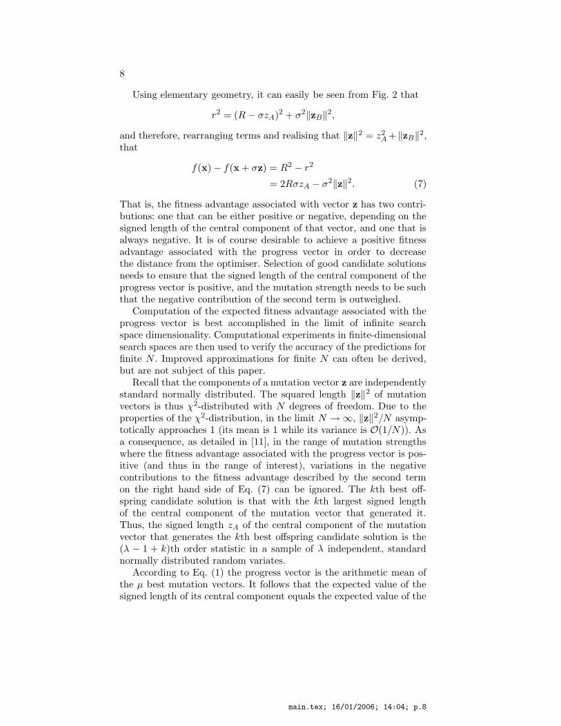
Using elementary geometry, it can easily be seen from Fig. 2 that

r2 = (R − σzA)2 + σ2‖zB‖2,

and therefore, rearranging terms and realising that ‖z‖2 = z2A +‖zB‖2,

that

f(x)− f(x + σz) = R2 − r2

= 2RσzA − σ2‖z‖2. (7)

That is, the fitness advantage associated with vector z has two contri-butions: one that can be either positive or negative, depending on thesigned length of the central component of that vector, and one that isalways negative. It is of course desirable to achieve a positive fitnessadvantage associated with the progress vector in order to decreasethe distance from the optimiser. Selection of good candidate solutionsneeds to ensure that the signed length of the central component of theprogress vector is positive, and the mutation strength needs to be suchthat the negative contribution of the second term is outweighed.

Computation of the expected fitness advantage associated with theprogress vector is best accomplished in the limit of infinite searchspace dimensionality. Computational experiments in finite-dimensionalsearch spaces are then used to verify the accuracy of the predictions forfinite N . Improved approximations for finite N can often be derived,but are not subject of this paper.

Recall that the components of a mutation vector z are independentlystandard normally distributed. The squared length ‖z‖2 of mutationvectors is thus χ2-distributed with N degrees of freedom. Due to theproperties of the χ2-distribution, in the limit N →∞, ‖z‖2/N asymp-totically approaches 1 (its mean is 1 while its variance is O(1/N)). Asa consequence, as detailed in [11], in the range of mutation strengthswhere the fitness advantage associated with the progress vector is pos-itive (and thus in the range of interest), variations in the negativecontributions to the fitness advantage described by the second termon the right hand side of Eq. (7) can be ignored. The kth best off-spring candidate solution is that with the kth largest signed lengthof the central component of the mutation vector that generated it.Thus, the signed length zA of the central component of the mutationvector that generates the kth best offspring candidate solution is the(λ − 1 + k)th order statistic in a sample of λ independent, standardnormally distributed random variates.

According to Eq. (1) the progress vector is the arithmetic mean ofthe µ best mutation vectors. It follows that the expected value of thesigned length of its central component equals the expected value of the

main.tex; 16/01/2006; 14:04; p.8

9

arithmetic mean of the (λ+1−µ)th through λth order statistics. Letting

Xi = z(i)A , Lemma 1 from Section 2.2 is thus immediately applicable

and the expected signed length of the central component of the progressvector is cµ/µ,λ. Moreover, it has been shown in [8] that

‖z(avg)‖2N

N→∞

=1

µ. (8)

The reduction in the squared length by a factor of 1/µ compared tothat of the mutation vectors being averaged results from the fact thatthe lateral components of the latter have no influence on the fitness ofthe candidate solutions and are thus uncorrelated. Averaging µ uncor-related random vectors of squared length 1 yields a random vector ofsquared length 1/µ. The averaging is beneficial as the negative termcontributing to the fitness advantage of the progress vector is reduced.In [8], that reduction has been termed the genetic repair effect.

Real-world optimisation problems often suffer from noise presentin the process of evaluating the quality of candidate solutions. Suchnoise can be a consequence of factors as varied as the use of MonteCarlo techniques, physical measurement limitations, or human inputin the selection process. As discussed in [1, 3], most frequently, noiseis modelled as an additive Gaussian term with mean zero and witha standard deviation σε that is referred to as the noise strength. Thenoisy objective function value of candidate solution y = x+σz then is

fε(y) = f(x)− 2RσzA + σ2‖z‖2 + σεzε

where zε is standard normally distributed and where the index in fε

indicates the measurement of the fitness value is disturbed by noise.Variations in the third term on the right hand side again lose signifi-cance as N → ∞. As both the second and fourth terms are normallydistributed, so is the noisy fitness advantage associated with vector z.

Noise has no influence on the squared length of the progress vector.However, it does have an influence on the signed length of that vector’scentral component. The candidate solutions selected to survive arethose with the largest values of 2RσzA − σεzε. The signed lengths ofthe central components of the mutation vectors are thus concomitantsof the order statistics that result from ranking the offspring candidate

solutions by their noisy objective function values. Letting Yi = z(i)A and

Zi = −(σε/2Rσ)z(i)ε , Lemma 2 from Section 2.2 is applicable and the

expected signed length of the central component of the progress vectoris

E[

z(avg)A

]

N→∞

=cµ/µ,λ√1 + ϑ2

,

main.tex; 16/01/2006; 14:04; p.9

10

where ϑ = σε/2Rσ is the noise-to-signal ratio that the strategy operatesunder. Notice that in general, the noise strength need not be constant,but instead it may vary across the search space.

3. The (µ/µ, λ)-ES on the Noisy Parabolic Ridge

In this section the performance of the (µ/µ, λ)-ES with isotropic mu-tations is studied on the parabolic ridge. The treatment of cumulativestep length adaptation is deferred until Section 4. The results pre-sented here generalise those derived in [19] by considering noise in theanalysis. In contrast to that reference, no attempt is made to includeN -dependent terms in the calculations. Numerical experiments are usedto illustrate that the accuracy of the results is good provided that Nis sufficiently large.

3.1. Expected Progress Vector

Even though the parabolic ridge described by objective function

f(x) = x1 −d

N

N∑

i=2

x2i x ∈ IRN , d > 0 (9)

has no finite optimum, maximisation is still a meaningful task if prog-ress along the ridge axis (i.e., in the x1-direction) is considered as aperformance measure. It is also worth pointing out that while in thedefinition used here the ridge axis is aligned with an axis of the coor-dinate system, that fact is irrelevant for a strategy that uses isotropicmutations such as those considered in the present paper. The coordinatesystem could be subjected to an arbitrary rigid transformation withoutaffecting the strategy’s performance.

Clearly, the parabolic ridge contains within it an (N−1)-dimensionalquadratic sphere. Similar to the decomposition of vectors described inSection 2.3, a mutation or progress vector z = (z1, z2, . . . , zN )T on theridge can be written as the sum of three mutually orthogonal vectorsthat are straightforward to obtain. Let z1 = (z1, 0, . . . , 0)

T and z2...N =(0, z2, . . . , zN )T denote the projections of z onto the hyperspaces withz2 = · · · = zN = 0 and z1 = 0, respectively. Furthermore, decomposez2...N into vectors zA and zB as done in Section 2.3 with (x1, 0, . . . , 0)

T

for x. Then z = z1 + zA + zB is a decomposition of z into mutuallyorthogonal components and z1, zA, and zB are referred to as the axial,central, and lateral components of z, respectively. See Fig. 3 for anillustration.

main.tex; 16/01/2006; 14:04; p.10

11

PSfrag replacements

x1x2

x3 x2 and x3

R

σzσzA

σzB

σz2...Nσz2...N

σz1

Figure 3. Decomposition of vector z into its axial component z1, central compo-nent zA, and lateral component zB for N = 3. The dashed lines indicate locationsof constant fitness.

Using the decomposition along with Eqs. (6) and (9), it follows thatthe fitness of candidate solution y = x + σz is

f(y) = x1 + σz1 −d

N

N∑

i=2

(xi + σzi)2

= x1 −d

N

N∑

i=2

x2i + σz1 −

d

N

(

2σN∑

i=2

xizi + σ2N∑

i=2

z2i

)

= f(x) + σz1 +d

N

(

2σRzA − σ2‖z2...N‖2)

(10)

where R = ‖x2...N‖ denotes the distance of the search point from the

ridge axis. If z is a mutation vector then ‖z2...N‖2/N N→∞

= 1 holds asseen in the discussion of the sphere model in Section 2.3. Introducingthe standardised distance from the ridge axis

ρ =2Rd

N

the noisy fitness of candidate solution y is thus

fε(y)N→∞

= f(x) + σz1 + ρσzA − σ2d + σεzε (11)

where zε is a standard normally distributed random variable reflectingthe noise present in the evaluation process and where σε denotes thenoise strength.

For the purpose of selection, offspring candidate solutions are rankedaccording their noisy fitness values. According to Eq. (1), the mutation

main.tex; 16/01/2006; 14:04; p.11

12

vectors of those µ of the offspring with the highest noisy fitness valuesare averaged arithmetically to form the progress vector. The axial,central, and lateral components of the progress vector are thus thearithmetic means of the respective components of the selected mutationvectors. The signed lengths of the axial and central components ofthe mutation vectors are standard normally distributed. As the kthbest offspring candidate solution is that with the kth largest value ofσz1 + ρσzA + σεzε (the other terms in Eq. (11) are identical for alloffspring), the signed lengths of both the axial components z1 and thecentral components zA of the mutation vectors are concomitants of theorder statistics that result from ranking candidate solutions accordingto their noisy fitness. Moreover, as all random variables in Eq. (11) arenormally distributed, and as the sum of two normally distributed ran-dom variables is again normally distributed, Lemma 2 from Section 2.2

is applicable. In particular, letting Yi = z(i)1 and Zi = (ρσz

(i)A +σεz

(i)ε )/σ,

it follows from Lemma 2 that the expected value of the signed lengthof the axial component of the progress vector is

E[

z(avg)1

]

N→∞

=cµ/µ,λ

√

1 + ϑ2 + ρ2(12)

where ϑ = σε/σ denotes the noise-to-signal ratio that the strategy

operates under. Similarly, letting Yi = z(i)A and Zi = (σz

(i)1 +σεz

(i)ε )/ρσ,

it follows from Lemma 2 that the expected value of the signed lengthof the central component of the progress vector is

E[

z(avg)A

]

N→∞

=cµ/µ,λ

√

1 + (σ2 + σ2ε )/ρ

2σ2

=ρcµ/µ,λ

√

1 + ϑ2 + ρ2. (13)

Finally, for the squared length of the combined central and lateralcomponents of the progress vector,

‖z(avg)2...N ‖2N

N→∞

=1

µ(14)

holds in analogy to the corresponding result in Eq. (8) for the spheremodel.

3.2. Distance from the Ridge Axis and Progress Rate

The expected values of the signed lengths of the axial and central com-ponents of the progress vector computed in Eqs. (12) and (13) dependon the standardised distance ρ of the search point from the ridge axis.

main.tex; 16/01/2006; 14:04; p.12

13

In the case that the mutation strength is constant, that distance varieswith time and either has a time-invariant limit distribution or divergesto ∞. Steps 1, 2, and 3 of the algorithm outlined in Section 2.1 definean iterated stochastic mapping

R(t+1)2 =N∑

i=2

(

xi + σz(avg)i

)2

= R(t)2 − 2R(t)σz(avg)A + σ2‖z(avg)

2...N ‖2

of distances from the ridge axis, where Eq. (6) has been used and wheresuperscripts indicate time. Multiplying by 4d2/N2 in order to switchto standardised distances yields evolution rule

ρ(t+1)2 = ρ(t)2 − 4d

N

(

ρ(t)σz(avg)A − σ2d

N‖z(avg)

2...N ‖2)

(15)

for the dynamical system. Consider the case that ρ does not diverge.In that case, iterating Eq. (15), the squared standardised distance tothe ridge axis tends towards and then fluctuates around a stationarylimit value. For given σ, σε, ρ, and λ, both the mean and the varianceof the term in parentheses are in O(1). Due to the presence of thefactor 4d/N that that term is multiplied with, for given mutation andnoise strengths fluctuations are of order O(1/N) and thus decreasewith increasing search space dimensionality. In the limit case N →∞,variances vanish altogether and all random variables can be replaced bytheir expected values. Using Eqs. (13) and (14) for the expected values

of z(avg)A and ‖z(avg)

2...N ‖2 and demanding that ρ(t+1) = ρ(t), Eq. (15) yields

ρ2σcµ/µ,λ√

1 + ϑ2 + ρ2=

σ2d

µ.

Introducing normalised quantities

σ∗ =σd

µcµ/µ,λand σ∗

ε =σεd

µcµ/µ,λ,

squaring, and rearranging terms yields the equivalent condition

ρ4 − σ∗2(

1 + ρ2)

− σ∗

ε2 = 0 (16)

that can be used to obtain the stationary standardised distance fromthe ridge axis. The following three subsections consider three differenttypes of dependency of the noise strength on the distance from theridge axis. More specifically, the cases that the noise strength is uniform

main.tex; 16/01/2006; 14:04; p.13

14

0.0

1.0

2.0

3.0

4.0

5.0

0.0 1.0 2.0 3.0 4.0

PSfrag replacements

mutation strength σ∗

stan

dar

dis

eddis

tance

ρ

σ∗

ε = 0.0σ∗

ε = 5.0

σ∗

ε = 10.0

Figure 4. Standardised distance ρ from the ridge axis plotted against normalisedmutation strength σ∗ for the case of uniform noise strength. The solid lines havebeen obtained from Eq. (17). The points represent results measured in runs ofthe (µ/µ, λ)-ES on the parabolic ridge in search spaces with N = 40 (+) andN = 400 (×). In all cases, µ = 3, λ = 10, and d = 1.0.

throughout the search space, that it increases quadratically with thedistance from the ridge axis, and that the rate of increase is cubicare examined. The cases have been chosen as they can be handledanalytically while at the same time exhibiting qualitatively differentcharacteristics and posing widely differing demands to the step lengthcontrol mechanism to be discussed in Section 4.

3.2.1. Uniform Noise StrengthConsider the case that the noise strength σε is uniform throughout thesearch space. Solving Eq. (16) yields

ρ2 N→∞

=σ∗2

2+

√

σ∗4

4+ σ∗2 + σ∗

ε2 (17)

for the squared standardised distance from the ridge axis. Figure 4illustrates how the accuracy of predictions made using Eq. (17) im-proves with increasing values of N by comparing with values measuredin runs of evolution strategies. Not shown here, greater values of µand λ generally require greater values of N in order to achieve thesame degree of accuracy. The quality of the approximation is largelyindependent of the strength of the noise present.

With the knowledge of the standardised distance from the ridge axisthus obtained, the performance of the (µ/µ, λ)-ES on the parabolic

main.tex; 16/01/2006; 14:04; p.14

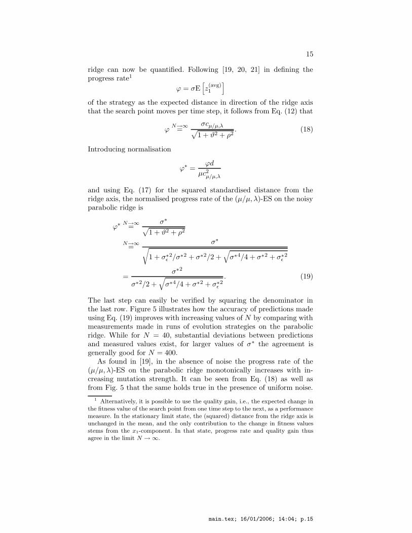
15

ridge can now be quantified. Following [19, 20, 21] in defining theprogress rate1

ϕ = σE[

z(avg)1

]

of the strategy as the expected distance in direction of the ridge axisthat the search point moves per time step, it follows from Eq. (12) that

ϕN→∞

=σcµ/µ,λ

√

1 + ϑ2 + ρ2. (18)

Introducing normalisation

ϕ∗ =ϕd

µc2µ/µ,λ

and using Eq. (17) for the squared standardised distance from theridge axis, the normalised progress rate of the (µ/µ, λ)-ES on the noisyparabolic ridge is

ϕ∗ N→∞

=σ∗

√

1 + ϑ2 + ρ2

N→∞

=σ∗

√

1 + σ∗

ε2/σ∗2 + σ∗2/2 +

√

σ∗4/4 + σ∗2 + σ∗

ε2

=σ∗2

σ∗2/2 +√

σ∗4/4 + σ∗2 + σ∗

ε2. (19)

The last step can easily be verified by squaring the denominator inthe last row. Figure 5 illustrates how the accuracy of predictions madeusing Eq. (19) improves with increasing values of N by comparing withmeasurements made in runs of evolution strategies on the parabolicridge. While for N = 40, substantial deviations between predictionsand measured values exist, for larger values of σ∗ the agreement isgenerally good for N = 400.

As found in [19], in the absence of noise the progress rate of the(µ/µ, λ)-ES on the parabolic ridge monotonically increases with in-creasing mutation strength. It can be seen from Eq. (18) as well asfrom Fig. 5 that the same holds true in the presence of uniform noise.

1 Alternatively, it is possible to use the quality gain, i.e., the expected change inthe fitness value of the search point from one time step to the next, as a performancemeasure. In the stationary limit state, the (squared) distance from the ridge axis isunchanged in the mean, and the only contribution to the change in fitness valuesstems from the x1-component. In that state, progress rate and quality gain thusagree in the limit N → ∞.

main.tex; 16/01/2006; 14:04; p.15

16

0.0

0.2

0.4

0.6

0.8

1.0

0.0 1.0 2.0 3.0 4.0

PSfrag replacements

mutation strength σ∗

pro

gres

sra

teϕ∗

σ∗

ε = 0.0

σ∗

ε = 5.0

σ∗

ε = 10.0

Figure 5. Normalised progress rate ϕ∗ plotted against normalised mutation strengthσ∗ for the case of uniform noise strength. The solid lines have been obtained fromEq. (19). The points represent results measured in runs of the (µ/µ, λ)-ES on theparabolic ridge in search spaces with N = 40 (+) and N = 400 (×). In all cases,µ = 3, λ = 10, and d = 1.0.

In addition to its beneficial effect for σε = 0, increasing σ reducesthe noise-to-signal ratio ϑ = σε/σ that the strategy operates under.For large mutation strengths that ratio tends to zero and according toEq. (19) the effects of noise on the progress rate vanish.

From Eqs. (17) and (19) and undoing the normalisations, for largemutation strengths the strategy operates at a standardised distance ofclose to ρ = σd/µcµ/µ,λ from the ridge axis and achieves a progress rate

of nearly ϕmax = µc2µ/µ,λ/d. Increasing the population size parameters

µ and λ thus decreases the stationary standardised distance ρ from theridge axis and increases the optimal progress rate ϕmax. Similar to whathas been found on the quadratic sphere [8, 11], a roughly linear increasein ϕmax can be achieved as a result of increasing λ provided that µ isincreased such that the ratio µ/λ remains unchanged. For large valuesof λ, a setting of µ = 0.270λ is optimal as it maximises µc2

µ/µ,λ. Larger

values of λ are beneficial and result in a linear speed-up if offspringcandidate solutions can be evaluated in parallel. Notice however thatEq. (19) holds only in the limit N → ∞. In finite-dimensional searchspaces, the rate of increase of ϕmax is sublinear in µ and λ, and theserial performance of the (µ/µ, λ)-ES suffers once the number of off-spring generated per time step is too large. It is not possible to derivequantitative recommendations with regard to the choice of λ from the

main.tex; 16/01/2006; 14:04; p.16

17

analysis presented here as all N -dependent terms have been left out ofthe calculations.

3.2.2. Quadratic Noise StrengthNext, consider the case that the noise strength increases quadraticallywith the distance from the ridge axis, i.e. that σε = ζρ2 for some ζ ≥ 0.We refer to ζ as the noise level. Equation (16) then reads

ρ4 − σ∗2(

1 + ρ2)

− ζ∗2ρ4 = 0

where ζ∗ = ζd/µcµ/µ,λ is the normalised noise level. Solving for thesquare of the standardised distance from the ridge axis yields

ρ2 N→∞

=σ∗2

2(1− ζ∗2)+

√

σ∗4

4(1 − ζ∗2)2+

σ∗2

1− ζ∗2 . (20)

For ζ∗ ≥ 1, there is no real-valued solution and the strategy fails totrack the ridge for any nonzero value of the mutation strength. In thatcase, the distance to the ridge axis diverges to ∞ and the resultingprogress rate (but not the quality gain!) approaches zero. If ζ ∗ < 1, thenthe resulting normalised progress rate is in close analogy to Eq. (19)

ϕ∗ N→∞

=σ∗

√

1 + ζ∗2ρ4/σ∗2 + ρ2

N→∞

=σ∗(1− ζ∗2)

σ∗/2 +√

σ∗2/4 + 1− ζ∗2. (21)

The dependence of the stationary distance ρ from the ridge axis andof the normalised progress rate ϕ∗ on ζ∗ are shown in Figs. 6 and 7.It can be seen that while the accuracy of the predictions is quite goodfor N = 400, the deviations in the lower dimensional search space withN = 40 are considerable. In contrast to the uniform noise case, thequality of the approximation also deteriorates with increasing levelsof noise present. The influence of the N -dependent terms cannot beneglected and better approximations remain to be derived in futurework. It is also worth noting that while Eqs. (20) and (21) suggest thatincreasing µ and λ makes it possible to deal with any amount of noisepresent (by driving ζ∗ to zero), this is an idealisation for N →∞ thatdoes not hold for finite N .

It can be seen from Figs. 6 and 7 that as in the case of uniformnoise strength, increasing the mutation strength is beneficial as it leadsto an increase in progress rate. However, unlike in the situation wherethe noise strength is uniform, in the quadratic case it is not possible

main.tex; 16/01/2006; 14:04; p.17

18

0.0

1.0

2.0

3.0

4.0

5.0

0.0 1.0 2.0 3.0 4.0

PSfrag replacements

mutation strength σ∗

stan

dar

dis

eddis

tance

ρ

ζ∗ = 0.0

ζ∗ = 0.5

ζ∗ = 0.75

Figure 6. Standardised distance ρ from the ridge axis plotted against normalisedmutation strength σ∗ for the case that the noise strength increases quadraticallywith the distance from the ridge axis. The solid lines have been obtained fromEq. (20). The points represent results measured in runs of the (µ/µ, λ)-ES on theparabolic ridge in search spaces with N = 40 (+) and N = 400 (×). In all cases,µ = 3, λ = 10, and d = 1.0.

to always achieve the same progress rate as in the absence of noise. Inthe uniform noise case, increasing the mutation strength results in ahigher signal strength that serves to drive the noise-to-signal ratio tozero. In the case that the noise strength increases quadratically withthe distance from the ridge axis however, the increased distance atwhich the ridge axis is tracked as a result of increasing σ also results inan increase in the noise strength that leads to the noise-to-signal ratiotend to a non-zero limit value. More specifically, for large mutationstrengths, the first term in the radicand in Eq. (20) dominates thesecond and the squared stationary standardised distance from the ridgeaxis is ρ2 = σ∗2/(1 + ζ∗2). The corresponding normalised progress rateis ϕ∗

max = 1 − ζ∗2 and thus decreases with increasing ζ∗. While theexact limit value is not well described by Eq. (21) unless N is verylarge, the qualitative behaviour of ρ2 and ϕ∗ is captured correctly byEqs. (20) and (21).

3.2.3. Cubic Noise StrengthFinally, consider the case that the noise strength increases cubicallywith the distance from the ridge axis, i.e. that σε = ζρ3. Equation (16)then reads

ρ4 − σ∗2(

1 + ρ2)

− ζ∗2ρ6 = 0 (22)

main.tex; 16/01/2006; 14:04; p.18

19

0.0

0.2

0.4

0.6

0.8

1.0

0.0 1.0 2.0 3.0 4.0

PSfrag replacements

mutation strength σ∗

pro

gres

sra

teϕ∗

ζ∗ = 0.0

ζ∗ = 0.5

ζ∗ = 0.75

Figure 7. Normalised progress rate ϕ∗ plotted against normalised mutation strengthσ∗ for the case that the noise strength increases quadratically with the distance fromthe ridge axis. The solid lines have been obtained from Eq. (21). The points representresults measured in runs of the (µ/µ, λ)-ES on the parabolic ridge in search spaceswith N = 40 (+) and N = 400 (×). In all cases, µ = 3, λ = 10, and d = 1.0.

and is thus no longer quadratic in ρ2 but cubic instead. For a givenvalue of ζ∗ and small σ∗, Eq. (22) has two nonnegative real roots, thesmaller of which corresponds to a stable fixed point of the cubic poly-nomial in Eq. (15). As σ∗ increases, the value of that fixed point growsuntil it coincides with the larger, unstable fixed point and subsequentlydisappears. The resulting effect on the standardised distance from theridge axis is illustrated in Fig. 8. The solid lines in that figure have beenobtained by numerically finding the root of Eq. (22) that corresponds tothe stable fixed point in the mapping of squared standardised distancesfrom the ridge axis. The line corresponding to ζ ∗ = 0.2 abruptly ends atσ∗ ≈ 2.4 as the stable fixed point disappears. With mutation strengthsbeyond this point, no stable limit state exists and the distance fromthe ridge axis diverges to ∞. For ζ∗ = 0.1, the point where the stablelimit state ceases to exist is beyond the range of mutation strengthsshown. The measurements from runs of evolution strategies that areincluded in the figure show that the behaviour can indeed be observedin practice.

While an explicit solution for the roots of the cubic equation exists,it is complicated and does not yield new insights. However, an upperbound on values of σ∗ that allow tracking the ridge can easily be de-rived. The two roots of the cubic polynomial in Eq. (22) are separated

by a local maximum at z = (1 +√

1− 3σ∗2ζ∗2)/3ζ∗2. That maximum

main.tex; 16/01/2006; 14:04; p.19

20

0.0

1.0

2.0

3.0

4.0

5.0

0.0 1.0 2.0 3.0 4.0

PSfrag replacements

mutation strength σ∗

stan

dar

dis

eddis

tance

ρζ∗ = 0.0

ζ∗ = 0.1

ζ∗ = 0.2

Figure 8. Standardised distance ρ from the ridge axis plotted against normalisedmutation strength σ∗ for the case that the noise strength increases cubically withthe distance from the ridge axis. The solid lines have been found by numericallyfinding the stable root of Eq. (22). The points represent results measured in runsof the (µ/µ, λ)-ES on the parabolic ridge in search spaces with N = 40 (+) andN = 400 (×). In all cases, µ = 3, λ = 10, and d = 1.0.

and with it the two roots do not exist if 1− 3σ∗2ζ∗2 < 0, making

σ∗ ≤ 1√3ζ∗

a necessary (though not sufficient) condition for being able to track theridge at a finite distance.

The case of noise that increases cubically with the distance from theridge axis is interesting as it presents a situation that is qualitativelydifferent from those considered so far. If the noise strength increasessuperquadratically with ρ, then the strategy is forced to track the ridgemore closely than it would in the cases considered above and thuscannot use arbitrarily large mutation strengths. The larger the level ofnoise present, the smaller the mutation strength needs to be in orderto be able to track the ridge. Figure 9 illustrates the dependence of theprogress rate on the mutation strength for several values of ζ ∗. It canbe seen that for ζ∗ 6= 0, increasing the mutation strength is beneficialup to some point. Beyond that point, the progress rate starts to declinebefore the strategy abruptly starts to lose its ability to track the ridge atall. As for the case of quadratic noise, the accuracy of the predictionsis quite good for N = 400. For N = 40 it is merely the qualitativedependence that is described correctly, and N -dependent terms willneed to be taken into account in order to derive recommendations with

main.tex; 16/01/2006; 14:04; p.20

21

0.0

0.2

0.4

0.6

0.8

1.0

0.0 1.0 2.0 3.0 4.0

PSfrag replacements

mutation strength σ∗

pro

gres

sra

teϕ∗

ζ∗ = 0.0

ζ∗ = 0.1

ζ∗ = 0.2

Figure 9. Normalised progress rate ϕ∗ plotted against normalised mutation strengthσ∗ for the case that the noise strength increases cubically with the distance from theridge axis. The solid lines have been obtained by inserting the numerically obtainedstable root of Eq. (22) into Eq. (18). The points represent results measured in runsof the (µ/µ, λ)-ES on the parabolic ridge in search spaces with N = 40 (+) andN = 400 (×). In all cases, µ = 3, λ = 10, and d = 1.0.

0.0

1.0

2.0

3.0

4.0

0.0 1.0 2.0 3.0 4.0

PSfrag replacements

noise level ζ∗

mutationstrength

σ∗

progress rate ϕ∗

0.0

0.2

0.4

0.6

0.8

1.0

0.0 1.0 2.0 3.0 4.0

PSfrag replacements

noise level ζ∗

mutation strength σ∗

progressrate

ϕ∗

Figure 10. Optimal normalised mutation strength σ∗ and resulting normalisedprogress rate ϕ∗ plotted against the normalised noise level ζ∗ for the case of noisethat increases cubically with the distance from the ridge axis. The graphs have beenobtained numerically using Eqs. (18) and (22).

regard to the choice of λ in finite-dimensional search spaces. Finally,Fig. 10 illustrates the dependence of the optimal mutation strengthand the resulting progress rate on ζ∗. That graphs in that figure havebeen obtained by numerically optimising Eq. (18) using the stablefixed point of Eq. (22) for ρ2. It can be seen that both the optimalmutation strength and the resulting progress rate decrease rapidly withincreasing levels of noise present.

main.tex; 16/01/2006; 14:04; p.21

22

4. Cumulative Step Length Adaptation

The calculations presented in Section 3 have considered the mutationstrength as a constant, exogenous quantity. In contrast, the algorithmoutlined in Section 2.1 adapts the mutation strength using the cumu-lative step length adaptation mechanism [18]. Cumulative step lengthadaptation on the noisy sphere model has been studied in [1, 5]. Thissection presents an analysis of the behaviour of cumulative step lengthadaptation of the noisy parabolic ridge. The analysis allows handlingall three forms of noise considered above.

4.1. Accumulated Search Path

It has been seen in Section 3.1 that the behaviour of the (µ/µ, λ)-ESwith static step length is described on the noisy parabolic ridge by aniterated stochastic mapping with the (standardised) distance from theridge axis as its only state variable and with Eq. (15) as its evolutionrule. Using cumulative step length adaptation introduces as furtherstate variables the axial and central lengths s1 and sA of the accumu-lated progress vector, the squared length ‖s‖2 of that vector, and themutation strength σ. That is, the algorithm described in Section 2.1defines a stochastic mapping

(ρ(t), s(t)1 , s

(t)A , ‖s(t)‖2, σ(t)) 7→ (ρ(t+1), s

(t+1)1 , s

(t+1)A , ‖s(t+1)‖2, σ(t+1))

that determines the behaviour of the strategy. The exact form of themapping can be inferred from Eqs. (3) and (4). The approach to com-puting stationary values is the same as that used in [1, 5] for the spheremodel and in Section 3 for the case of static step length: replace allquantities by their mean values and demand stationarity in that nochange occurs between time steps t and t + 1. Any terms that vanishin the limit N →∞ are dropped from the calculations. The approachyields useful approximations for large enough N as it can be observedthat fluctuations (quantified by the variation coefficients of the statevariables) decrease with increasing search space dimensionality. As inSection 3, computer experiments will be used to verify the quality ofthe approximations.

From Eq. (3), the evolution rule for the signed length of the axialcomponent of the accumulated progress vector reads

s(t+1)1 = (1− c)s

(t)1 +

√

µc(2− c)z(avg)1 .

Demanding stationarity yields

s1N→∞

=

√

µ(2− c)

cz(avg)1 (23)

main.tex; 16/01/2006; 14:04; p.22

23

for the mean value of that quantity, where z(avg)1 is given by Eq. (12).

Determining the signed length of the central component of the ac-cumulated progress vector is complicated by the fact that the directionof that component changes from one time step to the next. Similar toEq. (6), the signed length of the central component of the accumulatedprogress vector can be computed as

sA =s · (x− x)

R

where x = (x1, 0, . . . , 0) and where · denotes the inner product of twovectors. Using the assumption that the distance R from the ridge axisdoes not change along with Eq. (3) and the fact that according to Step 3of the algorithm in Section 2.1

x(t+1) − x(t+1) = x(t) − x(t) − σ(t)z(avg)2...N

it follows that

s(t+1)A =

1

R

(

(1− c)s(t) +√

µc(2 − c)z(avg))

·(

x(t) − x(t) − σ(t)z(avg)2...N

)

= (1− c)

(

s(t)A −

σ(t)

Rs(t) · z(avg)

2...N

)

+√

µc(2− c)

(

z(avg)A − σ(t)

R‖z(avg)

2...N ‖2)

.

Considering the first pair of parentheses on the right hand side, asthe direction of the lateral component of the progress vector z(avg) is

random, the product s(t) ·z(avg)2...N in the mean equals s

(t)A z

(avg)A . Moreover,

from Eq. (17) with ρ = 2Rd/N it follows that σ/R ≤ 2µcµ/µ,λ/N . Thus,

as 2µcµ/µ,λz(avg)A /N � 1, the second term in the pair of parentheses

disappears compared to the first in the limit N →∞ and can thus bedropped from the calculations. As a consequence, from the stationarityrequirement on the signed length of the accumulated progress vector’scentral component it follows that

sAN→∞

=

√

µ(2− c)

c

(

z(avg)A − σ

R‖z(avg)

2...N ‖2)

(24)

where z(avg)A and ‖z2...N‖2 are given by Eqs. (13) and (14), respectively.

Finally, again from Eq. (3), the overall squared length of the accu-mulated progress vector at time t + 1 is

‖s(t+1)‖2 = (1− c)2‖s(t)‖2

+ 2(1− c)√

µc(2− c)s(t) · z(avg) + µc(2 − c)‖z(avg)‖2.

main.tex; 16/01/2006; 14:04; p.23

24

As the direction of the lateral component of the progress vector z(avg) is

random, the product s(t) ·z(avg) in the mean equals s(t)1 z

(avg)1 +s

(t)A z

(avg)A ,

and, using Eqs. (23) and (24),

s(t)1 z

(avg)1 + s

(t)A z

(avg)A

N→∞

=

√

µ(2− c)

c

(

z(avg)1

2+ z

(avg)A

2− σ(t)

Rz(avg)A ‖z(avg)

2...N ‖2)

.

Demanding stationarity and solving for the squared length of the ac-cumulated progress vector thus yields

‖s‖2 N→∞

=2(1− c)

cµ

(

z(avg)1

2+ z

(avg)A

2− σ

Rz(avg)A ‖z(avg)

2...N ‖2)

+ µ‖z(avg)‖2. (25)

Altogether, Eqs (23), (24), and (25) together with Eqs. (12), (13),and (14) characterise the accumulated progress vector of the (µ/µ, λ)-CSA-ES on the noisy parabolic ridge for high search space dimension-ality.

4.2. Mutation Strength and Progress Rate

From Eq. (4), the stationarity requirement for the mutation strength issatisfied if and only if ‖s‖2 = N . The rightmost term on the right hand

side of Eq. (25) equals µ(z(avg)1

2+ ‖z(avg)

2...N ‖2), where z(avg)1 and ‖z(avg)

2...N ‖2are given by Eqs. (12) and (14), respectively. Due to the choice of the

cumulation coefficient c, the term involving z(avg)1 thus disappears for

N →∞ compared to both that involving ‖z(avg)2...N ‖2 and the first term on

the right hand side of Eq. (25). For large N , the stationarity conditionthus requires that

z(avg)1

2+ z

(avg)A

2=

σ

Rz(avg)A ‖z(avg)

2...N ‖2

and therefore, with Eqs. (12), (13), and (14) and the definition of ρ,that

(1 + ρ2)c2µ/µ,λ

1 + ϑ2 + ρ2=

2dσ

µ

cµ/µ,λ√

1 + ϑ2 + ρ2.

Using the definition of σ∗ and squaring both sides, this condition canbe written as

1 + 2ρ2 + ρ4 = 4σ∗2 + 4σ∗

ε2 + 4σ∗2ρ2.

main.tex; 16/01/2006; 14:04; p.24

25

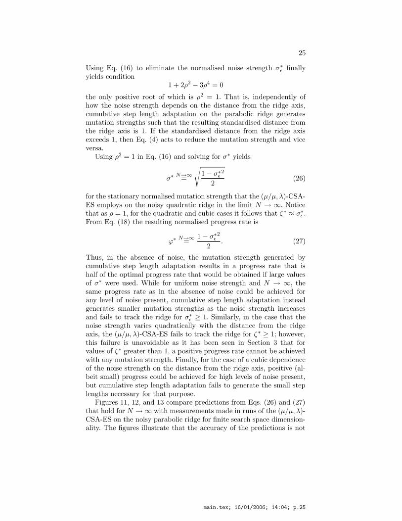
Using Eq. (16) to eliminate the normalised noise strength σ∗

ε finallyyields condition

1 + 2ρ2 − 3ρ4 = 0

the only positive root of which is ρ2 = 1. That is, independently ofhow the noise strength depends on the distance from the ridge axis,cumulative step length adaptation on the parabolic ridge generatesmutation strengths such that the resulting standardised distance fromthe ridge axis is 1. If the standardised distance from the ridge axisexceeds 1, then Eq. (4) acts to reduce the mutation strength and viceversa.

Using ρ2 = 1 in Eq. (16) and solving for σ∗ yields

σ∗ N→∞

=

√

1− σ∗

ε2

2(26)

for the stationary normalised mutation strength that the (µ/µ, λ)-CSA-ES employs on the noisy quadratic ridge in the limit N → ∞. Noticethat as ρ = 1, for the quadratic and cubic cases it follows that ζ ∗ ≈ σ∗

ε .From Eq. (18) the resulting normalised progress rate is

ϕ∗ N→∞

=1− σ∗

ε2

2. (27)

Thus, in the absence of noise, the mutation strength generated bycumulative step length adaptation results in a progress rate that ishalf of the optimal progress rate that would be obtained if large valuesof σ∗ were used. While for uniform noise strength and N → ∞, thesame progress rate as in the absence of noise could be achieved forany level of noise present, cumulative step length adaptation insteadgenerates smaller mutation strengths as the noise strength increasesand fails to track the ridge for σ∗

ε ≥ 1. Similarly, in the case that thenoise strength varies quadratically with the distance from the ridgeaxis, the (µ/µ, λ)-CSA-ES fails to track the ridge for ζ ∗ ≥ 1; however,this failure is unavoidable as it has been seen in Section 3 that forvalues of ζ∗ greater than 1, a positive progress rate cannot be achievedwith any mutation strength. Finally, for the case of a cubic dependenceof the noise strength on the distance from the ridge axis, positive (al-beit small) progress could be achieved for high levels of noise present,but cumulative step length adaptation fails to generate the small steplengths necessary for that purpose.

Figures 11, 12, and 13 compare predictions from Eqs. (26) and (27)that hold for N →∞ with measurements made in runs of the (µ/µ, λ)-CSA-ES on the noisy parabolic ridge for finite search space dimension-ality. The figures illustrate that the accuracy of the predictions is not

main.tex; 16/01/2006; 14:04; p.25

26

0.0

0.2

0.4

0.6

0.8

1.0

0.0 0.2 0.4 0.6 0.8 1.0 1.2

PSfrag replacements

noise strength σ∗

ε

mutationstrength

σ∗

progress rate ϕ∗

0.0

0.2

0.4

0.6

0.0 0.2 0.4 0.6 0.8 1.0 1.2

PSfrag replacements

noise strength σ∗

ε

mutation strength σ∗

progressrate

ϕ∗

Figure 11. Average normalised mutation strength σ∗ and normalised progressrate ϕ∗ of the (µ/µ, λ)-CSA-ES plotted against normalised noise strength σ∗

ε for thecase of uniform noise strength. The solid lines have been obtained from Eqs. (26)and (27), respectively. The points represent results measured in runs of the strat-egy on the parabolic ridge in search spaces with N = 40 (+) and N = 400 (×).Measurements have been made for µ = 3, λ = 10, and d = 1.0.

0.0

0.2

0.4

0.6

0.8

1.0

0.0 0.2 0.4 0.6 0.8 1.0 1.2

PSfrag replacements

noise level ζ∗

mutationstrength

σ∗

progress rate ϕ∗

0.0

0.2

0.4

0.6

0.0 0.2 0.4 0.6 0.8 1.0 1.2

PSfrag replacements

noise level ζ∗

mutation strength σ∗

progressrate

ϕ∗

Figure 12. Average normalised mutation strength σ∗ and normalised progressrate ϕ∗ of the (µ/µ, λ)-CSA-ES plotted against normalised noise level ζ∗ for thecase that the noise strength increases quadratically with the distance from the ridgeaxis. The solid lines have been obtained from Eqs. (26) and (27), respectively. Thepoints represent results measured in runs of the strategy on the parabolic ridge insearch spaces with N = 40 (+) and N = 400 (×). Measurements have been madefor µ = 3, λ = 10, and d = 1.0.

as good as it is for the case of static step length. Especially for thecase of cubic dependence of the noise strength on the distance fromthe ridge axis and N = 40 is the dynamic adaptation process unstableexcept for the smallest noise levels. However, it can also be seen thatthe accuracy of the predictions increases for increasing search spacedimensionality as expected, and that the qualitative dependence on themutation strength is described properly by Eqs. (26) and (27). TakingN -dependent terms into account in future work will allow making moreaccurate predictions and making quantitative recommendations withregard to the choice of µ and λ.

main.tex; 16/01/2006; 14:04; p.26

27

0.0

0.2

0.4

0.6

0.8

1.0

0.0 0.2 0.4 0.6 0.8 1.0 1.2

PSfrag replacements

noise level ζ∗

mutationstrength

σ∗

progress rate ϕ∗

0.0

0.2

0.4

0.6

0.0 0.2 0.4 0.6 0.8 1.0 1.2

PSfrag replacements

noise level ζ∗

mutation strength σ∗

progressrate

ϕ∗

Figure 13. Average normalised mutation strength σ∗ and normalised progressrate ϕ∗ of the (µ/µ, λ)-CSA-ES plotted against normalised noise level ζ∗ for thecase that the noise strength increases cubically with the distance from the ridgeaxis. The solid lines have been obtained from Eqs. (26) and (27), respectively. Thepoints represent results measured in runs of the strategy on the parabolic ridge insearch spaces with N = 40 (+) and N = 400 (×). Measurements have been madefor µ = 3, λ = 10, and d = 1.0.

5. Conclusions and Outlook

This paper has examined the effects of noise on the performance ofthe (µ/µ, λ)-ES on the quadratic ridge function class. Three forms ofnoise have been considered: uniform noise that has the same strengththroughout the search space, noise that increases quadratically with thedistance from the ridge axis, and noise where that dependence is cubic.Quantitative results have been derived in the limit N →∞, and theiraccuracy has been tested experimentally in finite-dimensional searchspaces. It has been seen that uniform noise can be effectively eliminatedby working with a large mutation strength and tracking the ridge ata great distance. If the noise increases quadratically with the distancefrom the ridge, then it is no longer possible to drive the noise-to-signalratio to zero by increasing the mutation strength, and above a certainnoise level tracking the ridge becomes impossible unless µ and λ areincreased. If the increase of the noise strength with the distance fromthe ridge is cubic, then positive progress can always be achieved, albeitonly with very small mutation strengths. Altogether, the three casesconsidered provide scenarios with widely differing characteristics thatpose different demands to step length adaptation mechanisms.

Then, the performance of cumulative step length adaptation hasbeen investigated for the three scenarios. It has been seen that inde-pendently of how the noise varies with the distance from the ridge axis,cumulative step length adaptation always generates mutation strengthsthat lead to the ridge being tracked at unit standardised distance. In theabsence of noise, the progress rate that is achieved is half of the optimal

main.tex; 16/01/2006; 14:04; p.27

28

progress rate. If there is noise present, then cumulative step lengthadaptation fails to generate useful step lengths if the noise exceeds unitstrength. The point where cumulative step length adaptation starts tofail can be deferred by increasing µ and λ.

This paper is but a first step toward an understanding of the be-haviour of adaptive evolution strategies on the ridge function class.The directions in which the results presented here can be extended arenumerous. First, it is desirable to obtain an improved understandingin finite-dimensional search spaces. Finite values of N place limits onhow far the population size parameters can beneficially be increasedand are instrumental for deriving recommendations with regard to thechoice of µ and λ. Such an understanding can be obtained by includingsome of the terms that have been dropped here in the analysis. Thechallenge is to determine what terms need to be considered, as well asthe treatment of fluctuations (i.e., of quantities that cannot simply bereplaced by their average values). Second, different forms of step lengthadaptation, such as mutative self-adaptation [9] or meta-ES [23] remainto be studied and compared with cumulative step length adaptation.For meta-ES, Herdy [17] provides empirical evidence for their usefulnessfor step length adaptation on the ridge. Third, other strategy variants,such as evolutionary gradient search strategies [24] or the (λ)opt-ESstudied in [2] on the sphere model remain to be considered. Of interestas well is the examination of ridge topologies other than the quadraticone. In the absence of noise and not considering step length adaptation,such an analysis has been presented in [10]. An finally, as pointed outby Whitley, Lunacek, and Knight [26], the ridge is a prime example forthe usefulness of nonisotropic mutations. Strategies such as the CMA-ES [16] are capable of learning the direction of the ridge axis. Afteradaptation of the covariance matrix is complete, the CMA-ES can trackthe ridge by generating mutation vectors that have large componentsin direction of the ridge and much smaller components in other direc-tions. This should prove especially useful if there is noise present thatincreases superquadratically with the distance from the ridge axis, andit will be interesting to see how noise affects the adaptation of thecovariance matrix.

Acknowledgements

This research has been supported by the Natural Sciences and Engi-neering Research Council of Canada (NSERC).

main.tex; 16/01/2006; 14:04; p.28

29

References

1. D. V. Arnold. Noisy Optimization with Evolution Strategies. Genetic Algo-rithms and Evolutionary Computation Series. Kluwer Academic Publishers,Boston, 2002.

2. D. V. Arnold. Optimal weighted recombination. In A. H. Wright, M. D. Vose,K. A. De Jong, and L. M. Schmitt, editors, Foundations of Genetic Algorithms

8, pages 215–237. Springer Verlag, Heidelberg, 2005.3. D. V. Arnold and H.-G. Beyer. Local performance of the (µ/µI , λ)-ES in a

noisy environment. In W. N. Martin and W. M. Spears, editors, Foundations

of Genetic Algorithms 6, pages 127–141. Morgan Kaufmann Publishers, SanFrancisco, 2001.

4. D. V. Arnold and H.-G. Beyer. A comparison of evolution strategies with otherdirect search methods in the presence of noise. Computational Optimization

and Applications, 24(1):135–159, 2003.5. D. V. Arnold and H.-G. Beyer. Performance analysis of evolutionary optimiza-

tion with cumulative step length adaptation. IEEE Transactions on Automatic

Control, 49(4):617–622, 2004.6. D. V. Arnold and H.-G. Beyer. Expected sample moments of concomitants of

selected order statistics. Statistics and Computing, 15(3):241–250, 2005.7. N. Balakrishnan and C. R. Rao. Order statistics: An introduction. In N. Bal-

akrishnan and C. R. Rao, editors, Handbook of Statistics, volume 16, pages3–24. Elsevier, Amsterdam, 1998.

8. H.-G. Beyer. Toward a theory of evolution strategies: On the benefit of sex —the (µ/µ, λ)-theory. Evolutionary Computation, 3(1):81–111, 1995.

9. H.-G. Beyer. Toward a theory of evolution strategies: Self-adaptation.Evolutionary Computation, 3(3):311–347, 1996.

10. H.-G. Beyer. On the performance of (1, λ)-evolution strategies for the ridgefunction class. IEEE Transactions on Evolutionary Computation, 5(3):218–235,2001.

11. H.-G. Beyer. The Theory of Evolution Strategies. Natural Computing Series.Springer Verlag, Heidelberg, 2001.

12. H.-G. Beyer, D. V. Arnold, and S. Meyer-Nieberg. A new approach for predict-ing the final outcome of evolution strategy optimization under noise. Genetic

Programming and Evolvable Machines, 6(1):7–24, 2005.13. H.-G. Beyer and H.-P. Schwefel. Evolution strategies — A comprehensive

introduction. Natural Computing, 1(1):3–52, 2002.14. H. A. David and H. N. Nagaraja. Concomitants of order statistics. In N. Bala-

krishnan and C. R. Rao, editors, Handbook of Statistics, volume 16, pages487–513. Elsevier, Amsterdam, 1998.

15. N. Hansen. Verallgemeinerte individuelle Schrittweitenregelung in der Evolu-

tionsstrategie. Mensch & Buch Verlag, Berlin, 1998.16. N. Hansen and A. Ostermeier. Completely derandomized self-adaptation in

evolution strategies. Evolutionary Computation, 9(2):159–195, 2001.17. M. Herdy. Reproductive isolation as strategy parameter in hierarchically or-

ganized evolution strategies. In R. Manner and B. Manderick, editors, Parallel

Problem Solving from Nature — PPSN II, pages 207–217. Elsevier, Amsterdam,1992.

18. A. Ostermeier, A. Gawelczyk, and N. Hansen. Step-size adaptation based onnon-local use of selection information. In Y. Davidor, H.-P. Schwefel, and

main.tex; 16/01/2006; 14:04; p.29

30

R. Manner, editors, Parallel Problem Solving from Nature — PPSN III, pages189–198. Springer Verlag, Heidelberg, 1994.

19. A. I. Oyman and H.-G. Beyer. Analysis of the (µ/µ, λ)-ES on the parabolicridge. Evolutionary Computation, 8(3):267–289, 2000.

20. A. I. Oyman, H.-G. Beyer, and H.-P. Schwefel. Where elitists start limping:Evolution strategies at ridge functions. In A. E. Eigen, T. Back, M. Schoenauer,and H.-P. Schwefel, editors, Parallel Problem Solving from Nature — PPSN V,pages 109–118. Springer Verlag, Heidelberg, 1998.

21. A. I. Oyman, H.-G. Beyer, and H.-P. Schwefel. Analysis of the (1, λ)-ES onthe parabolic ridge. Evolutionary Computation, 8(3):249–265, 2000.

22. I. Rechenberg. Evolutionsstrategie — Optimierung technischer Systeme nach

Prinzipien der biologischen Evolution. Friedrich Frommann Verlag, Stuttgart,1973.

23. I. Rechenberg. Evolutionsstrategie ’94. Friedrich Frommann Verlag, Stuttgart,1994.

24. R. Salomon. Evolutionary algorithms and gradient search: Similarities anddifferences. IEEE Transactions on Evolutionary Computation, 2(2):45–55,1998.

25. R. Salomon. The curse of high-dimensional search spaces: Observing prematureconvergence in unimodal functions. In Proc. of the 2004 IEEE Congress on

Evolutionary Computation, pages 918–923. IEEE Press,, Piscataway, NJ, 2004.26. D. Whitley, M. Lunacek, and J. Knight. Ruffled by ridges: How evolutionary

algorithms can fail. In K. Deb, R. Poli, W. Banzhaf, H.-G. Beyer, E. Burke,P. Darwen, D. Dasgupta, D. Floreano, J. Foster, M. Harman, O. Holland, P. L.Lanzi, L. Spector, A. Tettamanzi, D. Thierens, and A. Tyrell, editors, Ge-

netic and Evolutionary Computation — GECCO 2004, pages 294–306. SpringerVerlag, Heidelberg, 2004.

main.tex; 16/01/2006; 14:04; p.30