Exact, Efficient, and Complete

Arrangement Computation for Cubic Curves 1

Arno Eigenwillig a, Lutz Kettner a,

Elmar Schomer b, and Nicola Wolpert a

aMax-Planck-Institut fur Informatik

Stuhlsatzenhausweg 85, 66123 Saarbrucken, Germany

bJohannes-Gutenberg-Universitat Mainz, Institut fur Informatik

Staudingerweg 9, 55099 Mainz, Germany

Abstract

The Bentley-Ottmann sweep-line method can compute the arrangement of planarcurves, provided a number of geometric primitives operating on the curves are avail-able. We discuss the reduction of the primitives to the analysis of curves and curvepairs, and describe efficient realizations of these analyses for planar algebraic curvesof degree three or less. We obtain a complete, exact, and efficient algorithm forcomputing arrangements of cubic curves. Special cases of cubic curves are conics aswell as implicitized cubic splines and Bezier curves.

The algorithm is complete in that it handles all possible degeneracies such astangential intersections and singularities. It is exact in that it provides the mathe-matically correct result. It is efficient in that it can handle hundreds of curves witha quarter million of segments in the final arrangement. The algorithm has beenimplemented in C++ as an Exacus library called CubiX.

Key words: Arrangements, algebraic curves, sweep-line algorithm, robustness,exact geometric computation

Email addresses: arno@mpi-inf.mpg.de (Arno Eigenwillig),kettner@mpi-inf.mpg.de (Lutz Kettner), schoemer@uni-mainz.de (ElmarSchomer), wolpert@mpi-inf.mpg.de (Nicola Wolpert).1 Partially supported by the IST Programme of the European Union as a Shared-cost RTD (FET Open) Project under Contract No. IST-2000-26473 (ECG – Effec-tive Computational Geometry for Curves and Surfaces).

Article published in Computational Geometry 35 (2006) 36–73

1 Introduction

1.1 Problem Statement

The Bentley-Ottmann sweep-line method [9] can be used to compute the ar-rangement of planar curves. One only has to provide a number of geometricprimitives (break a curve into x-monotone pieces, given two curves computetheir intersections, compare two intersections or endpoints lexicographically,etc.). The “only” is the crux of the matter; not in principle, but in terms ofefficient realization.

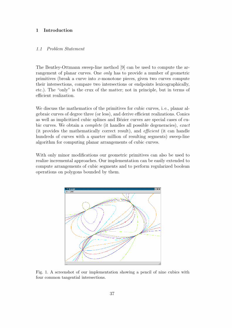
We discuss the mathematics of the primitives for cubic curves, i. e., planar al-gebraic curves of degree three (or less), and derive efficient realizations. Conicsas well as implicitized cubic splines and Bezier curves are special cases of cu-bic curves. We obtain a complete (it handles all possible degeneracies), exact(it provides the mathematically correct result), and efficient (it can handlehundreds of curves with a quarter million of resulting segments) sweep-linealgorithm for computing planar arrangements of cubic curves.

With only minor modifications our geometric primitives can also be used torealize incremental approaches. Our implementation can be easily extended tocompute arrangements of cubic segments and to perform regularized booleanoperations on polygons bounded by them.

Fig. 1. A screenshot of our implementation showing a pencil of nine cubics withfour common tangential intersections.

37

1.2 Related Work

Complete, exact, and efficient implementations for planar arrangements ofstraight line segments exist, e. g., in LEDA [62, ch. 10.7], and in the planarmap [34] and planar Nef-polyhedron [74] classes of CGAL. However, exist-ing implementations for curved objects are either incomplete, inexact, or notaimed at efficiency except for some recent work on circle and conic arcs (seebelow). For cubic curves we are not aware of any complete, exact, and efficientimplementation.

Our work is influenced by results from three different communities: computeraided geometric design (CAGD), computational geometry, and computer al-gebra. The problem of computing intersections of curves and surfaces has along history in CAGD. The CAGD community concentrates on approximatesolutions by numerical methods which cannot distinguish, e. g., between a tan-gential intersection and two intersections lying very close together. Completeand exact implementations have been addressed recently: MAPC [50] is a li-brary for exact computation and manipulation of algebraic curves. It offersarrangements of planar curves but does not handle all degenerate situations.Yap [82] uses separation bounds to make the traditional subdivision algo-rithm for the intersection of Bezier curves exact and complete in the presenceof tangential and almost-tangential intersections.

Arrangements, mostly of linear objects, are also a major focus in computa-tional geometry; see the survey articles of Halperin [43] and Agarwal/Sharir[2]. Many exact methods for curved objects have been formulated for theReal RAM model of computation [67], which allows unit-time operations onarbitrary real numbers and conceals the high cost of exact arithmetic withalgebraic numbers.

Sakkalis [70,71], Hong [45], and Gonzalez-Vega/Necula [42] analyze the topol-ogy of a single real algebraic curve. Their approaches, like ours, can be seenas special forms of Cylindrical Algebraic Decomposition [23,5]. However, theydo not consider the interaction between pairs of curves, and the full algebraicmachinery they deploy is not necessary for cubic curves. The recent text-book by Basu, Pollack, and Roy [8] is a very useful reference for the algebraicbackground of those methods and also contains a curve topology algorithm.Aspects of the crucial problem to capture behavior at irrational points byrational arithmetic were treated by Canny [20] (Gap Theorem) and Pedersen[66] (multivariate Sturm sequences).

Predicates for arrangements of circular arcs that reduce all computations tosign determination of polynomial expressions in the input data are treatedby Devillers et al. [26]. Recent work by Emiris et al. [31,32] discusses some

38

predicates on conics in this style. However, these approaches do not extendeasily to more complicated curves.

Exact, efficient, and complete algorithms for planar arrangements have beenpublished by Wein [77] and Berberich et al. [11] for conic segments, and byWolpert [78,73] for special quartic curves as part of a surface intersectionalgorithm. A generalization of Jacobi curves (used for locating tangential in-tersections) is described by Wolpert [79].

The work presented here follows the Master’s thesis of the first author [28]and has appeared as an extended abstract in [29].

1.3 Our Results

What are the difficulties in going from straight lines and straight line segmentsto conics and further on to cubic curves? The defining equations and thus thegeometry of the basic objects and the coordinates of their intersections becomemore complicated. For straight line segments with rational endpoints, all ver-tices in their arrangement have rational coordinates. In the case of curves, theintersections are solutions to systems of non-linear polynomial equations andthus, in general, irrational algebraic numbers. We review polynomials, alge-braic numbers, and elimination of variables among polynomial equations inSection 2.

The sweep-line algorithm works on x-monotone segments. Lines and line seg-ments are x-monotone, conics need to be split at points of vertical tangent,and cubic curves need to be split at points of vertical tangent and at singular-ities. These notions and other required elements of the geometry of algebraiccurves are introduced in Section 3. Cubic curves have a more diverse geome-try than conics. Its analysis is a separate step in our algorithm, explained inSection 4.1.

We turn to pairs of curves. Two lines intersect in a single point with rationalcoordinates. Two conics intersect in up to four points. Each of the intersectingconic arcs can be parametrized in the form y(x) using a single square root.In the case of a tangential intersection, the x-coordinate of the intersectioncan also be written as an expression involving a single square root. Therefore,previous work on conics [77,11] could make heavy use of the existing efficientmethods for arithmetic within FRE [48,18], the field of real root expressions.FRE is the closure of the integers under the operations +, −, ∗, /, and k

√for

arbitrary but fixed k; it is a subfield of the real algebraic numbers. However,the k

√operation is restricted to extracting real-valued roots, thus general

polynomial equations of degree ≥ 3 are not solvable in FRE, severely limitingits applicability to cubics. (The usability of recent additions for arithmetic

39

with all real algebraic numbers [55,19,72] remains to be investigated.) Hencewe need more powerful techniques. We discuss them and the geometric analysisof curve pairs in Section 4.2.

The central idea of our approach to curve and curve pair analyses is to exploitgeometric properties of cubic curves in order to avoid arithmetic with irrationalnumbers as far as possible.

In Section 5 we put everything together and discuss high-level issues of theBentley-Ottmann sweep for algebraic curves and how the required predicatesreduce to curve and curve pair analyses. This part applies to algebraic curvesof any degree.

We conclude with a discussion of running time from a theoretical (Section 6)and especially an experimental (Section 7) point of view. We point out thatthere is a full implementation of our algorithm.

2 Algebraic Foundations

The algorithmic handling of algebraic curves rests to a large extent on alge-braic operations. We give a concise summary of the existing results we use,just enough to make our presentation self-contained and accessible to non-experts in symbolic computation. This summary also provides the necessarycontext for describing the implementation choices we made.

As reference for the abstract algebra involved here we mention the textbookby Lang [54]. The algorithmic aspects are covered in the computer algebrabooks by Geddes/Czapor/Labahn [38], Akritas [4], Cohen [21], and von zurGathen/Gerhard [36]. The recent book by Basu/Pollack/Roy [8] combines theviewpoints of real algebraic geometry and computer algebra.

2.1 Rings and Fields

Recall the algebraic notions of ring and field. All fields considered in the sequelhave characteristic zero, i. e., contain the rational numbers Q. A ring in modernterminology is a commutative ring with unity. We additionally demand it tocontain the integers Z, and unless specifically stated otherwise, to be freeof zero divisors. With our terminology, every ring R possesses an essentiallyunique quotient field Q(R), i. e., a ⊆-minimal field containing R as a subring.For example, Q(Z) = Q.

We say d divides r and write d|r if there is c ∈ R such that r = cd. If u|1,

40

u is a unit of R. A non-unit r 6= 0 that cannot be written as product of twoother non-unit elements is called an irreducible element. A ring R is a uniquefactorization domain (UFD) if any non-zero non-unit element r possesses afactorization

r =k∏

i=1

pi (1)

into irreducible elements pi that is unique up to reordering the pi and multi-plying them by units. In any UFD R, the irreducible elements p are prime,meaning that for all r, s ∈ R we have p|rs ⇒ p|r∨ p|s. (For a proof, see [54,II.4].) Given r ∈ R and some irreducible element p, the maximal exponente ∈ N0 such that pe|r is called the multiplicity of p in r.

2.2 Polynomials

2.2.1 Basics

Adjoining an indeterminate x to a ring R yields the univariate polynomialring R[x]. We call f ∈ R[x] monic if its leading coefficient `(f) is 1. Iteratedadjunction of indeterminates leads to multivariate polynomials R[x1] · · · [xn] =R[x1, . . . , xn]. The units of R[x1, . . . , xn] are the units of R.

A multivariate polynomial can be seen recursively as a univariate polyno-mial in xn with coefficients in R[x1] · · · [xn−1], or flat as a sum of termsai1...inxi1

1 · · ·xinn . Its total degree deg(f) is max{i1 + . . . + in | ai1...in 6= 0}.

A polynomial is homogeneous if all its terms have the same total degree.Otherwise, it decomposes uniquely as a sum of its homogeneous parts f =f0 + f1 + . . . + fdeg(f) where fd is homogeneous of degree d. The d-th orderterms fd are called constant, linear, quadratic, etc., part of f , for d = 0, 1, 2, . . .,respectively.

Let k ≤ n and ξ ∈ Rk. Substituting values ξ1, . . . , ξk for x1, . . . , xk homomor-phically maps f 7→ f |ξ = f(ξ1, . . . , ξk, xk+1, . . . , xn) ∈ R[xk+1, . . . , xn].

A polynomial f ∈ R[x1, . . . , xn] is called xn-regular if it contains a term cxdeg(f)n

with 0 6= c ∈ R. Its degree does not change when substituting values forx1, . . . , xk, k < n. The product of two xn-regular polynomials is xn-regular.Any factor of an xn-regular polynomial is xn-regular.

2.2.2 Unique factorization and the GCD

Let K be a field. The univariate polynomial ring K[x] is a Euclidean ring byvirtue of division with remainder: For any two polynomials f, g ∈ K[x], g 6= 0,

41

there exists a unique quotient q and remainder r in K[x] such that

f = qg + r, deg(r) < deg(g). (2)

The constructive proof of this proposition yields a simple and reasonably ef-ficient algorithm to compute these quantities. Iff g|f , then it produces theremainder 0 and the quotient f/g.

Recall that in any ring R a greatest common divisor (gcd) of two elementsr, s ∈ R is an element d ∈ R such that d|r∧ d|s, and d′|r∧ d′|s ⇒ d′|dfor all d′ ∈ R. To compute a gcd in K[x], there is the Euclidean Algorithm:Given two non-zero polynomials f, g ∈ K[x], repeatedly replace one of larger(or equal) degree with its remainder modulo the other one, until zero occursas remainder. The last non-zero remainder d is gcd(f, g). By accumulatingintermediate results, the Extended Euclidean Algorithm (EEA) additionallycomputes Bezout factors p, q ∈ K[x] with the property d = pf + qg. See [38,2.4], [36, 3.2], [80, 2.2] or [21, 3.2.1].

The EEA demonstrates that K[x] is a principal ideal domain and hence aUFD [54, II.4, V.4]. Thus any non-zero polynomial f ∈ K[x] has a unique (upto order) factorization

f = `(f) ·k∏

j=1

qej

j (3)

into its leading coefficient and powers of pairwise distinct monic irreduciblefactors qj with their respective multiplicities ej > 0. This follows from (1) bynormalizing and grouping factors.

Let us now consider the divisibility properties of polynomials over a UFD R. Inthis setting, non-unit constant factors are relevant. For a non-zero polynomialf ∈ R[x], define the content cont(f) of f as the gcd of its coefficients. Ifcont(f) = 1, then f is called primitive.

Proposition 1 (Gauss’ Lemma)Let R be a UFD. Let f, g ∈ R[x] be non-zero. Then cont(fg) = cont(f) cont(g).

For a proof, see [54, V.6]. The following easy corollary relates the divisibilityproperties of R[x] and Q(R)[x].

Corollary 2 Let R be a UFD, and let f, g ∈ R[x] be non-zero polynomials.Then the following conditions are equivalent:

(i) g|f in R[x],

(ii) g|f in Q(R)[x] and cont(g)|cont(f) in R.

In particular, these two notions of divisibility by g are equivalent if g is prim-itive.

Continuing that line of thought [54, V.6], one obtains:

42

Theorem 3 (Gauss’ Theorem)If R is a UFD, then R[x1, . . . , xn] is a UFD.If K is a field, then K[x1, . . . , xn] is a UFD.

Hence any non-zero f ∈ K[x1, . . . , xn] factors essentially uniquely into coprimeirreducible factors with their respective multiplicities. (We shall meet suchirreducible factors again later on for n = 2 as components of curves.) It followsthat there exists gcd(f, g) for non-zero f, g ∈ K[x1, . . . , xn]. The following easycorollary to Proposition 1 is useful for its computation.

Corollary 4 Let R be a UFD, and let f, g ∈ R[x] be non-zero polynomials.Then cont(gcd(f, g)) = gcd(cont(f), cont(g)).

Suppose we can compute gcds in a UFD R. Then we can also compute gcd(f, g)for non-zero f, g ∈ R[x]: Because of Corollary 2, gcd(f, g) is, up to a constantfactor, the gcd of f, g regarded as elements of Q(R)[x], and we can computethat with the Euclidean Algorithm. Using Corollary 4, the error in the constantfactor can then be corrected by adjusting the content to gcd(cont(f), cont(g)).This allows us to compute gcds, for example, in Z[x]; and, by a recursiveapplication of this approach, in R[x1, . . . , xn] or K[x1, . . . , xn]. We refer to [38]for details.

An efficient implementation of this scheme employs Q(R) only conceptuallyand keeps all coefficients in R in order to avoid costly fractional arithmetic.To obtain (constant multiples of) remainders in R[x], one changes Euclideandivision into pseudo division by replacing f with `(g)deg(f)−deg(g)+1f in (2), sothat all divisions of coefficients become possible within R. To curb coefficientgrowth, one needs to predict a large constant factor of each remainder anddivide it out. To do this, we use the subresultant method due to Collins [22]and Brown/Traub [17]. It is described by Loos [59, 4.5], Brown [16], and Knuth[51, pp. 428+]. (A subsequent improvement has been obtained by Lickteig andRoy [56, §4] [57, Thm. 4.1], see also [58], [8, 8.3] or [30].)

2.2.3 Multiplicities and Derivatives

Whenever we have unique factorization into irreducibles, we can formulate theweaker notion of square-free factorization, or factorization by multiplicities aswe like to call it. Take (3) and group factors qi with equal multiplicities m = ei

into one factor sm:

f = `(f) ·maxi ei∏

m=1

smm, where sm =

∏

ei=m

pi (4)

The factors sm are square free, meaning that all their irreducible factors occurwith multiplicity 1; and any two sm are coprime, i. e., the two have no non-unit

43

factor in common. Define the square-free part of f as∏

m sm.

The significance of this weaker form of polynomial factorization lies in the rela-tive ease of computing it, using derivatives. For a polynomial f =

∑ni=0 aix

i wedefine its (formal) derivative as f ′ :=

∑ni=1 iaix

i−1. For multivariate polynomi-als f ∈ R[x1, . . . , xn], partial derivatives are defined accordingly and denotedby subscripts like fx1x2 . Partial differentiation of polynomials w. r. t. differentvariables commutes. The result of differentiating f exactly r ≥ 0 times w. r. t.some choice of variables is called an r-th partial derivative of f . The columnvector of all first partial derivatives of f is the gradient ∇f := (fx1, . . . , fxm

)T

of f .

The relation of derivatives and multiplicities is rooted in the following result.

Proposition 5 Let K be a field, let f ∈ K[x] be a non-zero polynomial, andlet f = `(f)

∏Mm=1 sm

m be its square-free factorization. Then

gcd(f, f ′, . . . , f (k)) =M∏

m=k+1

sm−km (up to units) (5)

for all k ≥ 0. In particular, the square-free part of f is f/ gcd(f, f ′).

Proof. By induction on k. The base case k = 0 is obvious. The inductivestep is performed by applying the following observation separately to eachirreducible factor of f : Let f = grh, r ≥ 1 so that g is irreducible and doesnot divide h. Then f ′ = rg′gr−1h + grh′ = (rg′h + gh′)gr−1, and g does notdivide rg′h + gh′, because it divides gh′ but neither g′ (which is of smallerdegree) nor h (by definition). 2

Square-free factorization, like gcd computation, does not depend on the choiceof K and applies equally to all fields containing the coefficients of f . Fur-thermore, the statement of the proposition remains valid for an xn-regularpolynomial f ∈ K[x1, . . . , xn] when derivatives are taken w. r. t. xn.

The relation (5) of multiplicities and derivatives allows us to compute a square-free factorization of f ∈ K[x] or of f ∈ R[x] for a UFD R by repeateddifferentiation and gcd computation. Yun’s Algorithm [38, 8.2] does this in aclever way to keep the coefficients of intermediate polynomials small.

This algorithm prompts an implementation choice concerning the computa-tion of gcd-free parts; that is, passing from a pair (f, g) of polynomials to thetriple (f/d, g/d, d) where d = gcd(f, g). We choose the obvious implementa-tion (compute d and divide by it). The alternative of executing the ExtendedEuclidean Algorithm and obtaining the gcd-free parts as cofactors of the zero

44

polynomial at the end of the polynomial remainder sequence [8, Thm. 10.13]did not seem to offer a better performance for the univariate instances of theproblem met in our application.

2.2.4 Roots of Polynomials

Let K be a field, and let f ∈ K[x]. As a consequence of division with re-mainder, we have that f(ξ) = 0 at some point ξ ∈ K iff x − ξ is one of theirreducible factors of f . This allows us to define the multiplicity of ξ as a rootor zero of f as the multiplicity of x− ξ as a factor of f . Furthermore, it allowsus to conclude that a polynomial f of degree n has at most n roots, countedwith multiplicity, and that an irreducible factor p of f is either linear, andhence corresponds to a zero of f , or has degree larger than 1 and no zeroesin K.

A field K is called algebraically closed if the second alternative does not occur.For every field K there exists an essentially unique ⊆-smallest algebraicallyclosed field K containing K, called the algebraic closure of K. Each elementof K is a root of some polynomial with coefficients in K. See [54, VII.2]. Thealgebraic closure of the reals R is the field C = R(i) of complex numbers. Asa proper subset, it contains the algebraic closure Q of the rationals Q.

Let ϑ be an algebraic number. Q(ϑ) denotes the ⊆-minimal subfield of Q con-taining ϑ. Among all monic polynomials from Q[x] that vanish at ϑ, thereis one of minimal degree. It is uniquely determined and called the minimalpolynomial f of ϑ. The degree of ϑ is defined as deg(f). The kernel of theevaluation homomorphism Q[x] → Q(ϑ), x 7→ ϑ, consists precisely of the mul-tiples of f , so that the field Q(ϑ) is isomorphic to the quotient ring Q[x]/(f),see [54, II.1, VII.1]. Now consider all roots ϑ1 := ϑ, ϑ2, . . . , ϑd of f . They arealgebraically indistinguishable insofar as Q(ϑi) and Q(ϑj) are isomorphic forany 1 ≤ i, j ≤ d; hence a polynomial equation with rational coefficients is sat-isfied by none or by all of the ϑi. We call the ϑi the algebraic conjugates of ϑ.Observe the analogy with the usual complex conjugation defined by replacingthe imaginary unit i with the other root −i of its minimal polynomial x2 + 1.

The notion of algebraic conjugacy extends to n-tuples ξ of algebraic numbersby choosing an algebraic number ϑ such that all ξi are rational expressions inϑ, and ϑ is conversely a rational expression in ξ1, . . . , ξn. (Such ϑ exists andis called the primitive element of Q(ξ1) · · · (ξn), see [54, VII.6] for an abstractand [60, Thm. 11] for a constructive proof.) The conjugates of ξ are the n-tuples obtained by replacing ϑ with its conjugates. No two distinct conjugatesof ϑ produce the same ξ. If ξ is a solution to a system of polynomial equationswith rational coefficients, then any of the deg(ϑ) many conjugates is a solutionas well.

45

2.3 Resultants

Intersecting two algebraic curves f and g essentially means solving a systemf(x, y) = g(x, y) = 0 of two polynomial equations. For this purpose, we willneed some results from elimination theory.

2.3.1 The Sylvester Resultant

We start by looking at the solvability of a system of two equations in onevariable.

Proposition 6 Let K be a field. Let f =∑m

i=0 aixi, am 6= 0, and g =∑n

i=0 bixi, bn 6= 0 be two polynomials in K[x]. Then the following conditions

are equivalent:

(i) f and g have a common zero in the algebraic closure K.

(ii) deg(gcd(f, g)) > 0.

(iii) There are non-zero u, v ∈ K[x] with deg(u) < deg(g) and deg(v) <deg(f) such that uf + vg = 0.

(iv) The determinant of the (n + m) × (n + m) Sylvester matrix

Syl(f, g) =

am · · · · · · a0

. . .. . .

am · · · · · · a0

bn · · · · · · b0

. . .. . .

bn · · · · · · b0

(6)

vanishes.

Proof. The equivalence of (i)–(iii) is easy. The equivalence of (iii) and (iv)follows by linear algebra, noting that the transpose Syl(f, g)T is the matrix ofa linear map taking a pair of coefficient vectors from Kn × Km, representingdegree-bound polynomials u and v, to the coefficient vector in Kn+m thatrepresents the polynomial uf + vg. The determinant vanishes iff there is anon-zero vector that is mapped to zero. See [25, 3.5] for more details. 2

The determinant det(Syl(f, g)) is called the resultant res(f, g, x) of f and gwith respect to x. The following proposition is not surprising in the light of(i) ⇔ (iv):

46

Proposition 7 Let K be a field. Consider the two non-zero polynomials f =am

∏mi=1(x − αi) and g = bn

∏nj=1(x − βj) in K[x]. It holds that

res(f, g, x) = anmbm

n

m∏

i=1

n∏

j=1

(αi − βj). (7)

Proofs can be found in [54, V.10] [60, Thm. 1] [21, 3.3.2].

Proposition 6 can be read as a statement on the Euclidean Algorithm executedfor f and g: Iff det(Syl(f, g)) vanishes, the polynomial remainder sequence off and g ends with zero before a constant gcd is reached. In fact, there is a deepconnection between subdeterminants of the Sylvester matrix and polynomialremainder sequences; see [59], [80, 3.6–3.9] or [8, 8.3]. We state only its mostprominent part, using the following notion:

Let K be a field, and let f, g ∈ K[x] be two non-zero polynomials with degreeshigher than k ≥ 0. Then the k-th subresultant 2 sresk(f, g, x) of f and g isdefined as the determinant of the matrix obtained from Syl(f, g) by deletingthe last 2k columns of the matrix and the last k rows of each of the twoparallelograms of coefficients.

Proposition 8 With f , g and k as above, the remainder sequence computedby the Euclidean algorithm for f and g contains a remainder of degree k iffthe k-th subresultant of f and g does not vanish. In particular,

sresi(f, g, x) = 0 for all 0 ≤ i < k ⇐⇒ deg(gcd(f, g)) ≥ k. (8)

A proof appears in [36, 6.10]. In the sequel, we will only need (8) specializedto k = 2; for this a direct proof is given in [4, Thm. 5.2.5].

2.3.2 Elimination with the Resultant

Now consider bivariate polynomials f, g ∈ K[x, y]. Proposition 6 can help usto solve f = g = 0 when we view f and g as polynomials in Q(K[x])[y]. Thesolution proceeds in two stages [25, 3.1]:

(1) The projection step in which we determine the partial solutions ξ, i. e.,the values of x for which the system f = g = 0 permits a solution (ξ, η).

2 The literature is divided between two definitions of subresultant. This article usesthe notion of a scalar subresultant. In the context of polynomial subresultants, theseare called principal subresultant coefficients. See [37] for a systematic comparison.See [59], [80, 3.6–3.9], [8, 8.3] and [30] for the theory of polynomial subresultants.

47

(2) The extension step in which we extend a partial solution x = ξ by allpossible values η of y such that f(ξ, η) = g(ξ, η) = 0.

In this setting, res(f, g, y) is a polynomial from K[x], and we might hope thatits zero set is the set of partial solutions ξ, on the grounds that a vanishing re-sultant indicates solvability of f |ξ = g|ξ = 0. However, the definition of the re-sultant depends on the (univariate) degrees of f and g, and these degrees dropwhen ξ is a zero of both `(f) and `(g). Then the Sylvester matrix Syl(f, g)|ξevaluated at ξ has a leftmost column full of zeroes, and so res(f, g, y)(ξ) = 0irrespective of ξ being a partial solution or not. Because of these extraneouszeroes, forming the resultant and evaluation in inner variables do not commutein general. However, if one of the polynomials is y-regular, everything is fine:

Proposition 9 Let K be a field, and let f, g ∈ K[x, y] be non-zero polynomi-als. Furthermore, let f be y-regular. Then for all ξ ∈ K the two conditions

(i) res(f, g, y)(ξ) = 0

(ii) There is η ∈ K such that f(ξ, η) = g(ξ, η) = 0

are equivalent.

Proof. We show that res(f, g, y)(ξ) = 0 is equivalent to res(f |ξ, g|ξ, y) = 0:Observe that Syl(f, g)|ξ contains Syl(f |ξ, g|ξ) as a lower right submatrix S.The d := deg(g) − deg(g|ξ) ≥ 0 columns left of S are zero below the diagonaland contain the constant diagonal entries `(f) 6= 0. Thus det(Syl(f, g)|ξ) =`(f)d det(Syl(f |ξ, g|ξ)), proving the claim. 2

This proposition extends in the obvious fashion to subresultants and theirproperty from Proposition 8.

When intersecting two curves, we aim for finitely many intersection points, sowe want to obtain a resultant which is not the zero polynomial.

Proposition 10 Let K be a field, and let f, g ∈ K[x, y] be non-zero polyno-mials. Then res(f, g, y) 6= 0 iff f and g have no common factor of positivedegree in y.

Proof. Recall from §2.2.2 that K[x] is a UFD. Hence Corollary 2 impliesthat f and g have no common factor of positive univariate degree as ele-ments of K[x][y] iff they have no common factor of positive univariate degreeas elements of Q(K[x])[y]. By Proposition 6, this is in turn equivalent tores(f, g, y) 6= 0. 2

48

Another practical concern relates to computations over the field of real num-bers R which is not algebraically closed. A real zero of res(f, g, y) may arisefrom a complex solution whose x-coordinate happens to be real. However,complex solutions come in pairs of complex conjugates. We will later guaran-tee uniqueness of solutions extending a given x-coordinate, so that real zeroesof res(f, g, y) are certain to come from real solutions.

2.3.3 Computing the Resultant

We have considered three options for computing the resultant of two polyno-mials f and g (up to sign):

(1) Compute the determinant of the Sylvester matrix Syl(f, g) defined above.This is the most obvious approach.

(2) Compute the determinant of the Bezout matrix Bez(f, g) defined below.This determinant is smaller and hence faster to compute.

(3) Compute a polynomial remainder sequence of f and g with the subresul-tant algorithm mentioned in §2.2.2. It computes subresultants incremen-tally along with the remainder sequence and uses them to curb coefficientgrowth; in particular, it computes the zeroth subresultant, which is theresultant.

In computing the determinant of a matrix with entries from a ring (in our case:integers or polynomials), it is preferable to avoid arithmetic with fractions forthe sake of efficiency. We have considered two choices for fraction-free deter-minant computations, namely, the algorithms of Gauss-Bareiss [21, 2.2.3] andBerkowitz 3 [68]. Gauss-Bareiss needs O(n3) arithmetic operations, includingdivisions that are possible within the ring of matrix entries; whereas Berkowitzneeds O(n4) arithmetic operations, none of them divisions. (Here, n is the rowand column dimension of the matrix.)

Our main application of resultants concerns y-regular bivariate polynomialsf, g ∈ Z[x][y] (viewed recursively) of degree at most 3. For this specific setting,with our implementations of the various alternatives, and with our benchmarkdata, we have observed that Berkowitz’ method for determinant computationis faster than Gauss-Bareiss, despite the asymptotics; and that evaluatingthe Bezout determinant with Berkowitz is faster than using the Sylvesterdeterminant or a subresultant remainder sequence. This is consistent with theresults of a recent study by Abdeljaoued et al. [1] for polynomials with higherdegrees and more inner variables.

3 This naming follows Rote [68, 2.8]. Others have attributed this algorithm toSamuelson.

49

Hence let us take a look at the Bezout matrix of two polynomials f, g ∈ K[x]both having degree m. Consider the polynomial f(x)g(z)−f(z)g(x) involvingthe new indeterminate z. It vanishes whenever x = z and therefore is divisibleby x − z. The quotient is

Λ(x, z) :=f(x)g(z) − f(z)g(x)

x − z=

m−1∑

i,j=0

cij xizj. (9)

The Bezout matrix of f and g is the m × m coefficient matrix Bez(f, g) :=(cij)

m−1i,j=0 of Λ. The book by Gelfand/Kapranov/Zelevinsky [39, 12.1] records

the following classical results:

Proposition 11 Let K be a field. Let f =∑m

i=0 aixi and g =

∑ni=0 bix

i be twopolynomials in K[x] of degrees m and n, resp., where m ≥ n.The entries of the Bezout matrix Bez(f, g) = (cij)

m−1i,j=0 are given by

cij =min(i,j)∑

k=0

[k, i + j + 1 − k], where [i, j] := aibj − ajbi, (10)

with the convention that ai = 0 for i > m and bi = 0 for i > n.The determinant of the Bezout matrix is

det(Bez(f, g)) = ±am−nm res(f, g, x). (11)

For m > n, the extraneous power of am in (11) can be avoided by forming ahybrid Bezout matrix of size m × m that consists of n Bezout-like rows andm − n Sylvester-like rows [27] [46]. We compute the resultant of f and g asdeterminant of this hybrid Bezout matrix using Berkowitz’ method.

The k-th subresultant can be expressed as an (m − k) × (m − k) subde-terminant of the (hybrid) Bezout matrix [27] [46]. This is how we computesubresultants. 4

We shall give two further references: The (sub)resultant property of (sub)de-terminants of the Bezout matrix is derived from first principles (i. e., withoutreference to the Sylvester matrix) by Goldman et al. [41]. The general Bezoutconstruction of resultants to eliminate several variables at once is treatedextensively by Bikker and Uteshev [12], including an explicit discussion of thesubresultant properties in the univariate case considered here. 5

4 The recent article [1] explains how to obtain all subresultants from one executionof Berkowitz’ method. While quite interesting in general, this would not gain a lotin our setting where m ≤ 3, k ≤ 1.5 Be warned that the matrix B considered in [12] differs from our Bezoutiant

Bez(f, g) by a change of basis.

50

2.4 Finding and Handling Roots of Polynomials

2.4.1 Root Isolation

On the algorithmic side, our main concern about roots is to determine the realroots of a polynomial f ∈ Q[x] in terms of isolating intervals with rationalboundaries. An interval [l, r] ⊆ R is called an isolating interval for a rootξ ∈ R of f ∈ R[x] if {x ∈ [l, r] | f(x) = 0} = {ξ}.

Before anything else, we make the coefficients of f integral and factor f bymultiplicities (see §2.2.3). Then we determine the zeroes of each square-freefactor separately.

We shortcut the factorization by multiplicities if res(f, f ′, x) 6≡ 0 modulo someprime, because res(f, f ′, x) 6= 0 is equivalent to f being already square free(see §2.2.3 and §2.3.1). Checking this condition modulo a prime small enoughto allow arithmetic in a double’s mantissa (following [15]) is much fasterthan computing gcd(f, f ′) = 1 from a polynomial remainder sequence overthe integers. In analogy to floating-point filters, we call this a modular filter.Squarefreeness is the expected case in our uses of root finding. The modularfilter allows us to handle this case efficiently with high probability, and it issimpler to implement than a full-blown modular gcd algorithm.

After factorization, we process each square-free factor∑n

i=0 aixi separately. We

compute an interval [−B, B] enclosing all its real roots as follows: Determine

k0 := min

{k ≥ 0

∣∣∣∣∣ |an| 2nk >n−1∑

i=0

|ai| 2ik

}(12)

by successively trying k = 0, 1, 2, 3, . . .; then take B = 2k0 (see [63, p. 144]).

To perform the actual root isolation, we use the Descartes Method, 6 a divide-and-conquer approach based on Descartes’ Rule of Signs. Its modern form goesback to Collins and Akritas [24], see also Krandick [52] and Rouilliler/Zim-mermann [69].

Proposition 12 (Descartes’ Rule of Signs)Let f ∈ R[x] be a non-zero polynomial with exactly p positive real roots(counted with multiplicities) and exactly v sign variations in its coefficientsequence. Then v − p is non-negative and even.

Proofs can be found in [4, Thm. 7.2.6], [63, Thm. 5.5], and [53]. A sign variationin a sequence a0, . . . , an of real numbers is a pair of indices 0 ≤ i < j ≤ n

6 The designation “Uspensky’s Method” is common but incorrect [3].

51

such that sign(ai) sign(aj) = −1 and ai+1 = . . . = aj−1 = 0. In other words,the number of sign variations is obtained by deleting all zeroes and countinghow many pairs of adjacent numbers have opposite signs.

If v = 0 or v = 1, then v is known to be the exact number of positive realroots. If v > 1, this count might include pairs of complex-conjugate roots closeto the positive real axis.

Descartes’ Rule extends to the number of real roots of f in an arbitrary openinterval ]l, r[6= R, l, r ∈ R∪{±∞} by applying it to the composition f ◦T witha Mobius transformation T (x) = ax+b

cx+dtaking ]0, +∞[ to ]l, r[, see [4, 7.3.2].

(A reversed bracket indicates exclusion of the boundary point.)

The Descartes Method works as follows: Starting from the initial intervalenclosing all roots, recursively subdivide intervals at their midpoint until eachinterval under consideration is known to be isolating (v = 1) or empty (v = 0).The crux is to prove that v ∈ {0, 1} will hold eventually. The oldest proof isfrom A. J. H. Vincent (1836). We refer the reader to [53] for a rediscoveredresult of Ostrowski [65] that gives a particularly strong partial converse.

An alternative to the Descartes Method is provided by Sturm Sequences. Theseare polynomial remainder sequences of f and f ′ with special arrangements forsigns of the remainders (see [4, 7.2.2], [63, 5.4.1] or [80, chap. 7]), so unlessthe modular filter lets us skip that step, we essentially do compute a Sturmsequence for f during its square-free factorization. Nevertheless, we do not useit for root isolation. An empirical study by Johnson [47] indicates that rootisolation based on Sturm Sequences is often inferior to the Descartes Method,even if the cost of obtaining the Sturm sequence is excluded.

2.4.2 Representing and ordering real algebraic numbers

Let the polynomial f0 ∈ Q[x] have a real root ϑ ∈ R. The procedure of §2.4.1computes a representation ϑ =(f, [l, r]) for it consisting of a square-free factorf ∈ Z[x] of f0 and an isolating interval with boundaries l, r ∈ Q. (In the fieldof symbolic computation, this representation is standard [60].) Except for thedegenerate case l = r = ϑ, we make sure ϑ ∈]l, r[.

We want to compare numbers of that form. A key step is the bisection of a non-degenerate isolating interval [l, r] at a point t ∈]l, r[. The squarefreeness of fimplies that f ′(ϑ) 6= 0, hence the continuously differentiable function f : R →R does not have a local extremum at ϑ and consequently changes sign at ϑ. Theabsence of further zeroes in [l, r] implies that ±1 = sign(f(l)) 6= sign(f(r)) =∓1. By comparing sign(f(t)) against sign(f(r)), 0, and sign(f(l)), we candecide whether ϑ ∈]l, t[, ϑ = t, or ϑ ∈]t, r[, and refine [l, r] to [l, t], [t, t] or[t, r], respectively.

52

Let ϑ1 =(f1, [l1, r1]) and ϑ2 =(f2, [l2, r2]) be two algebraic numbers which weintend to compare. If their isolating intervals overlap, we bisect each interval atthe boundaries of the other interval it contains to make the two intervals non-overlapping or equal. The order of two algebraic numbers with non-overlappingisolating intervals is apparent from their interval boundaries.

So let us assume that by now [l, r] := [l1, r1] = [l2, r2] with l < r. The polyno-mials f1 and f2 are square free and each has exactly one zero in [l, r]. Considerd := gcd(f, g), which is also square free. If sign(d(l)) 6= sign(d(r)), there is acommon zero ϑ1 = ϑ2 in [l, r] and we are done. Otherwise, d has no zero in[l, r], hence ϑ1 6= ϑ2, and we alternately refine their isolating intervals [li, ri]by bisection at the midpoint 1

2(li + ri) until they are non-overlapping. Termi-

nation is guaranteed by the fact that the interval lengths converge to 0, sothat their sum has to drop below |ϑ1 − ϑ2| eventually.

After a comparison of ϑ1 and ϑ2, the isolating intervals in their representationsare replaced by their refinements. If we have computed a non-constant gcd d,we also replace each fi by d or fi/d, respectively, whichever vanishes at ϑi, asis discernible from the sign change.

As before in §2.4.1, the idea of a modular filter is applicable. When comparingtwo algebraic numbers ϑ1 and ϑ2 of unrelated origin, the expected case isthat their defining polynomials are coprime. Hence before computing d :=gcd(f1, f2), our implementation checks whether res(f1, f2, x) 6≡ 0 modulo someprime (see §2.3.1). If this holds, we know d = 1. More on such optimizationscan be found in [44].

A variation of the method above allows to decide for ϑ =(f, [l, r]) whetherg(ϑ) = 0 or not: Compute d := gcd(f, g) and decide (by inspecting signs at land r) whether d vanishes at ϑ or not.

This representation of real algebraic numbers can be seen as a delayed formof numerical root finding with a portion of symbolic computation to han-dle equality accurately. Subsequent comparisons benefit from the refinementsdone earlier. Past inequality results are cached in the form of non-overlappingisolating intervals. The refinement of interval boundaries in a comparison ofunequal numbers ϑ1 < ϑ2 computes a rational number r ∈]ϑ1, ϑ2[∩Q alongthe way.

One can implement a union-find scheme to cache equality. This causes alllogical consequences of transitivity, reflexivity and symmetry of = to be ev-ident from unitedness. When uniting ϑ1 = ϑ2, replace the isolating intervals[l1, r1], [l2, r2] by their intersection. All logical consequences of transitivity of> previously reflected by [l1, r1] or [l2, r2] are also reflected by their intersec-tion. Thus, any logical consequence of a sequence of three-valued comparisonsof algebraic numbers with union can afterwards be read off without further

53

interval refinements.

We will need one more operation on algebraic numbers, namely, refining theisolating interval [l, r], l 6= r, of a zero ϑ of f against all zeroes of anothersquare-free polynomial g ∈ Z[x] different from ϑ. To achieve this, refine [l, r]by bisection until one of two conditions holds: Either Descartes’ Rule of Signsimplies the absence of a zero of g in the interval; or Descartes’ Rule of Signsimplies the existence of exactly one zero of g in the interval, and a sign changeof gcd(f, g) between the boundaries implies the existence of a common zerowithin the interval. (This zero must then be unique and identical to ϑ.)

For this operation, we want to retain an interval containing ϑ in its interior, sothe special case of hitting a zero exactly with the bisection point needs to beresolved by choosing another bisection point. The modular coprimality checkmentioned above applies here, too.

2.4.3 Computing with square roots

In a few special cases of the geometric analyses of the next section, we need tocompute with square roots

√D, D > 0, although most of the analyses (in par-

ticular the generic cases) are performed with integer and rational arithmeticalone. Two approaches exist for computing with square roots:

Separation bound number types like CORE::Expr [48] and leda::real [18].These number types support algebraic expressions, among others those builtup with field operations and

√from integer operands. They implement com-

parisons by guaranteed numerical approximations combined with separationbounds to determine at which point the precision suffices to detect equal-ity. Comparisons work best for expressions of small nesting depth and largedifference in value.

Symbolic representation. The general method of computing modulo the min-imal polynomial of an algebraic number (as mentioned in §2.2.4, cf. [60])reduces in this case to the high-school “pencil and paper” representationQ(

√D) = {a+b

√D | a, b ∈ Q} with the obvious implementation of field oper-

ations. After checking that D is not a square, one has a+b√

D = a′+b′√

D ⇔(a, b) = (a′, b′). This representation is preferable for processes like the Eu-clidean Algorithm in Q(

√D)[x], because there is no issue of growing expression

trees.

Our implementation of the geometric analyses from Section 4 uses the sym-bolic representation for algebraic algorithms. CORE::Expr or leda::real areused to compare root expressions, but it turns out that at those occasionsthe expressions will always be unequal. Here we just reuse their numericalapproximation routines but do not rely on separation bounds. See §4.2.4, case

54

“m = 4”, for an example how the use of both representations is combined.

3 Geometry of Algebraic Curves

This section summarizes those elements of the geometry of algebraic curvesthat are necessary for our purposes. There are many books on algebraic curves.Mostly, we follow Gibson’s excellent introduction [40]. The classic book byWalker [76] is a very useful and well-readable source. Further references arethe textbooks by Bix [13] and Cox/Little/O’Shea [25] and also the advancedbooks by Brieskorn/Knorrer [14] and Fulton [35].

3.1 Basics

Let K be a field. An affine algebraic curve (or just curve) is a non-constantbivariate polynomial f ∈ K[x, y], up to multiplication by a non-zero scalar.Often, we do not distinguish a curve f from its vanishing locus VK(f) :={(x, y) ∈ K2 | f(x, y) = 0}. We assume the reader is familiar with theprojective plane, projective algebraic curves F (x, y, z), and the correspon-dence between affine and projective curves by homogenization F (x, y, z) =zdeg(f)f(x/z, y/z) and dehomogenization f(x, y) = F (x, y, 1). (If not, see [40].)

Let A be an affine change of coordinates. Recall that A(VK(f)) = VK(f ◦A−1)because f(v) = 0 ⇔ (f ◦ A−1)(Av) = 0. All quantities we define belowtransform in the obvious fashion under coordinate changes.

Let f ∈ K[x, y] be an algebraic curve, and let K be the algebraic closure ofK. The polynomial f ∈ K[x, y] factors essentially uniquely into coprime irre-ducible factors pi with multiplicities ei > 0 analogous to (3). This correspondsto a decomposition of the zero set f into subsets pi, each of which we call an(irreducible) component of f with multiplicity ei.

Let v ∈ K2

be a point. The smallest m ≥ 0 such that there is an m-th partialderivative of f not vanishing at v is called the multiplicity mult(v; f) := mof v on f . In particular, mult(v; f) > 0 ⇔ v ∈ f . (Notice that f on theleft denotes the polynomial and on the right its vanishing locus.) By Taylorexpansion around v = (v1, v2), the multiplicity is the degree of the lowest-order terms of f expressed in powers of (x + v1) and (y + v2). From thischaracterization, it is immediate that

mult(v; gh) = mult(v; g) + mult(v; h); (13)

in particular, the multiplicity of a point is at least the sum of the multiplicities

55

of the components containing it. We call the points of multiplicity 1 the regularpoints of f . The points v of multiplicity ≥ 2, i. e., those with ∇f(v) = (0, 0),are called singular.

The linear factors over K of the lowest-order terms of f expressed in powersof (x + v1) and (y + v2) are called the tangents of f at v. A point is calledvertical if it has a vertical tangent. If v is regular, the unique tangent of f atv has the normal vector ∇f(v) and hence coincides with the notion of tangentfrom differential geometry.

Multiplicities of components are irrelevant for the zero set, hence we simplifymatters and demand f to be square free from now on.

Proposition 13 Almost all points v of a square-free y-regular algebraic curvef satisfy fy(v) 6= 0.

Proof. Given y-regularity, squarefreeness is equivalent to coprimality of fand fy (cf. §2.2.3). Hence res(f, fy, y) 6= 0 has only finitely many zeroes ξ, andthere are only finitely many points (ξ, η) of f . 2

Corollary 14 Almost all points of a square-free algebraic curve are regular.

Now we turn to the intersection of two coprime algebraic curves f, g ∈ K[x, y].Again, a notion of multiplicity will be important. By coprimality, f∩g is finite.A generic choice of coordinates puts the points of f ∩ g into bijective corre-spondence with the roots of res(f, g, y). We define the intersection multiplicitymult(v; f, g) of f and g at an intersection point v ∈ f ∩ g as the multiplicityof its x-coordinate v1 as a root of res(f, g, y), and as 0 for v /∈ f ∩ g. This def-inition is independent of the concrete choice of generic coordinates, but thatis not obvious, see [25, 8.7] or [14, 6.1]. This definition extends to projectivealgebraic curves by dehomogenization. Inspecting the degree of the resultantused in the definition above [40, 14.4] yields:

Theorem 15 (Bezout’s Theorem)Let K be an algebraically closed field, and let F, G ∈ K[x, y, z] be two coprimeprojective algebraic curves. Then they have exactly deg(F ) deg(G) intersectionpoints in the projective plane over K, counted with multiplicities.

Corollary 16 Let K be a field, and let f, g ∈ K[x, y] be two coprime affinealgebraic curves. Then they have at most deg(res(f, g, y)) intersection pointsin K2, counted with multiplicities, and deg(res(f, g, y)) ≤ deg(f) deg(g).

Intersection multiplicity depends on the multiplicity of the point on eithercurve [40, 14.5]:

56

Proposition 17 (Multiplicity Inequality)Let K be a field, and let v ∈ K2 be a point. Let f, g ∈ K[x, y] be two coprimealgebraic curves. Then mult(v; f, g) ≥ mult(v; f) mult(v; g), and equality holdsiff f and g have no common tangent at v.

In particular, the tangent of f at a regular point v is the unique line h withm := mult(v; f, h) ≥ 2. Generically, one has m = 2. In the special case m > 2,the regular point v is called a flex. Unless f contains a line component, thenumber of flexes is finite and bounded in terms of deg(f), see [40, 13.1].

3.2 Arcs of an Algebraic Curve

From now on, consider a y-regular curve f over the field R. Its vanishing locusis a closed subset f ⊆ R2. Since the set f ∩ fy of critical points is finite, f \ fy

is an open subset of f . From the Implicit Function Theorem, it follows thatevery connected component of f \ fy is a parametrized curve

γi : ]li, ri[ → R2 (14)

x 7→ (x, ϕi(x))

with some analytic function ϕi (called the implicit function) and intervalboundaries li, ri ∈ R ∪ {±∞}. In particular, every connected component off \ fy is a C∞-manifold of dimension 1 which is homeomorphic to an openinterval. We call the topological closure Ai := cl(γi(]li, ri[)) in R2 of each suchcomponent an arc of f . Since f is closed, Ai ⊆ f .

A generic change of coordinates makes fy(v) 6= 0 for a regular point v, demon-strating that f is a manifold around a critical point v that is not a singularpoint of f . A singular point v, however, is singular and hence critical in anycoordinate system.

The parametrization (14) involves a function ϕi which can be expressed asa convergent power series locally around any x in its domain. Such a powerseries is a special case of the more general notion of Puiseux series (a kindof series involving fractional powers of x) that allow parametrizations even atcritical points, see [76, IV.] and [14].

The intersection multiplicity of two curves, defined above in terms of resul-tants, measures the similarity of these implicit power series.

Proposition 18 Let K be R or C. Let f, g ∈ K[x, y] be two coprime y-regularalgebraic curves. Let v ∈ K2 be an intersection point of f and g that is criticalon neither of them. Then mult(v; f, g) is the smallest exponent d for whichthe coefficients of (x − v1)

d in the implicit power series of f and g around v

57

disagree.

Proof. (Idea only.) Choose a generic coordinate system. Consider f and gas univariate polynomials in y whose zeroes can be written as power seriesin x − v1. Apply Proposition 7 to see that the multiplicity of v1 as zero ofres(f, g, y) is the vanishing order of the intersecting pair (α(x−v1)−β(x−v1))of arcs. See [76, Thm. 5.2] for a generalization and its proof. 2

The following corollary is immediate.

Corollary 19 In the situation of Proposition 18 for K = R, the two arcs off and g intersecting at a point v change sides iff mult(v; f, g) is odd.

By changing coordinates, the proposition and its corollary extend to intersec-tions in non-singular critical points.

Now let us inspect the endpoints of an arc Ai := cl(γi(]li, ri[)) more closely.The y-regularity of f implies that f has no vertical asymptotes. If ri < +∞,then Ai has a right endpoint (ri, limx→ri

ϕi(x)) ∈ R2 which is a critical pointof f . If ri = +∞ then Ai has a right endpoint at infinity. We use analogousdefinitions for the left endpoint.

Criticality of a point (r, s) can be characterized in terms of substituting avertical line in parametric form t 7→ (r, s + t) info f . Taylor’s formula yields:

f(r + 0, s + t) = f(r, s) + fy(r, s)t +1

2fyy(r, s)t

2 + . . . (15)

We obtain:

Lemma 20 Let f ∈ K[x, y] be a y-regular algebraic curve, and let (r, s) ∈ K2.Then the following two statements are equivalent:

(i) The point (r, s) is an intersection of f and fy.

(ii) The polynomial f(r, y) ∈ K[y] has a multiple root at y = s.

It follows immediately that no two critical points on a curve of degree ≤ 3 canhave the same x-coordinate.

Let us now distinguish several kinds of critical points. A critical point (r, s)of f is either a singular or a regular point of f . In the latter case, the tangenth to f at (r, s) is the vertical line h = x − r. By reasoning analogous toProposition 18, we see that mult((r, s); f, h) = mult(0; f(r, s + t)). From (15)we obtain that (r, s) is a flex iff fyy(r, s) = 0. If (r, s) is not a flex, it followsfrom Corollary 19 that f is locally on one side of the vertical tangent at (r, s),

58

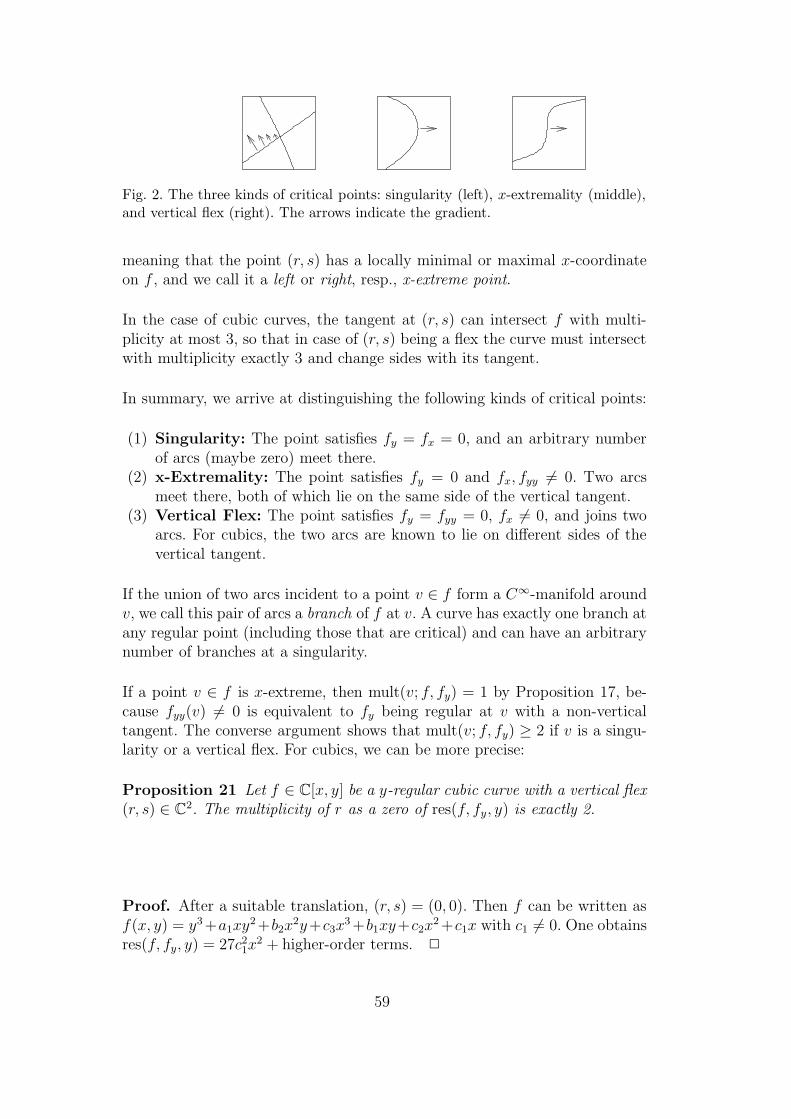
Fig. 2. The three kinds of critical points: singularity (left), x-extremality (middle),and vertical flex (right). The arrows indicate the gradient.

meaning that the point (r, s) has a locally minimal or maximal x-coordinateon f , and we call it a left or right, resp., x-extreme point.

In the case of cubic curves, the tangent at (r, s) can intersect f with multi-plicity at most 3, so that in case of (r, s) being a flex the curve must intersectwith multiplicity exactly 3 and change sides with its tangent.

In summary, we arrive at distinguishing the following kinds of critical points:

(1) Singularity: The point satisfies fy = fx = 0, and an arbitrary numberof arcs (maybe zero) meet there.

(2) x-Extremality: The point satisfies fy = 0 and fx, fyy 6= 0. Two arcsmeet there, both of which lie on the same side of the vertical tangent.

(3) Vertical Flex: The point satisfies fy = fyy = 0, fx 6= 0, and joins twoarcs. For cubics, the two arcs are known to lie on different sides of thevertical tangent.

If the union of two arcs incident to a point v ∈ f form a C∞-manifold aroundv, we call this pair of arcs a branch of f at v. A curve has exactly one branch atany regular point (including those that are critical) and can have an arbitrarynumber of branches at a singularity.

If a point v ∈ f is x-extreme, then mult(v; f, fy) = 1 by Proposition 17, be-cause fyy(v) 6= 0 is equivalent to fy being regular at v with a non-verticaltangent. The converse argument shows that mult(v; f, fy) ≥ 2 if v is a singu-larity or a vertical flex. For cubics, we can be more precise:

Proposition 21 Let f ∈ C[x, y] be a y-regular cubic curve with a vertical flex(r, s) ∈ C2. The multiplicity of r as a zero of res(f, fy, y) is exactly 2.

Proof. After a suitable translation, (r, s) = (0, 0). Then f can be written asf(x, y) = y3 +a1xy2 +b2x

2y+c3x3 +b1xy+c2x

2 +c1x with c1 6= 0. One obtainsres(f, fy, y) = 27c2

1x2 + higher-order terms. 2

59

3.3 Classification of Cubic Curves

In the following paragraphs, we classify square-free real algebraic curves f ∈Q[x, y] of degree at most 3 with respect to their decomposition into compo-nents as well as number and kind of their singularities. The statements belowfollow from three sources:

• The textbook classification of conics and cubics [40] up to complex-projec-tive changes of coordinates.

• Conjugacy arguments to demonstrate that something is real or rational oralgebraic of at most a certain degree. For example, let the homogenization Fof f have exactly three singularities in the complex-projective plane. Theyare the solutions of Fx = Fy = Fz = 0. Complex solutions come in pairs ofconjugates, so one of the three solutions must be real. Algebraic solutionsof degree d come in groups of d conjugates (as discussed in §2.2.4), so thenumber of solutions, in this case 3, bounds their algebraic degree.

• Real-projective changes of coordinates to bring cubic curves with a singu-larity into one of three normal forms [13, Thm. 8.4] that expose the realgeometry of the singularities.

3.3.1 Lines and Conics

Let f ∈ Q[x, y] be a line, i. e., deg(f) = 1. It is irreducible, real, and it possessesno singularities.

Let f ∈ Q[x, y] be a conic. It is either irreducible or a pair of two distinctlines. An irreducible conic possesses no singularities and is either the emptyset (like x2 + y2 + 1) or one of ellipse, parabola, or hyperbola.

By (13) in conjunction with Bezout’s Theorem, a line pair f = g1g2 has aunique singularity in the projective plane, i. e., the unique intersection pointv of its two components g1 and g2, which is rational but may lie at infinity.The two tangents at v are g1 and g2. If they are real, v is a crunode, and tworeal branches intersect at v. If they are complex, v is an acnode, which is anisolated point of f in the real plane.

3.3.2 Irreducible Cubics

Let f ∈ Q[x, y] be an irreducible cubic. It has at most one singular point v inthe projective plane. If v exists, f is called singular, otherwise non-singular.

The unique singularity v of a singular irreducible cubic f is rational but maylie at infinity. The curve f has exactly mult(v; f) = 2 tangents at v. If the

60

(a) (b) (c)

(d) (e) (f)

Fig. 3. Kinds of singularities: (a) acnode, (b) crunode, (c) cusp, (d) tacnode,(e) real triple point, (f) complex triple point

tangents are distinct, v is a crunode (two real branches and two real tangents)or an acnode (two complex-conjugate branches and tangents). If there is onedouble tangent, it is real, and v is called a cusp. At a cusp, two arcs convergefrom one side and do not continue in the real plane. (They come out complex-conjugate on the other side.)

3.3.3 Cubics with several components

Let f ∈ Q[x, y] be a cubic that is not irreducible. Then it has two components(a line and an irreducible conic) or three components (three lines). Since linesand irreducible conics have no singularities, by (13) all singularities of f areintersections of its components. Some of these singularities may lie at infinity.

Assume f = gh consists of a line g and an irreducible conic h. By Bezout’sTheorem, g and h intersect in exactly two complex-projective points withoutcommon tangent or in exactly one point with a common tangent. In the formercase, the two intersections may be complex-conjugates, so that there are nosingularities in the real plane, or two real crunodes. In the latter case, g is atangent to h at the unique intersection point, and the resulting intersectionis a tacnode. By uniqueness, a tacnode is rational. The two crunodes arerational, or they are algebraic of degree 2 and conjugates of each other. Bothcomponents g and h have rational coefficients, because g = y + ax + b is theunique solution to res(y + ax + b, f, y) = 0 and thus rational, and then thesame holds for h = f/g.

Now assume f = g1g2g3 consists of three distinct lines. Exactly one or three ofthem are real; and in both cases, two or three of them might have algebraically

61

conjugate equations.

If these three lines are concurrent at one point v ∈ g1 ∩ g2 ∩ g3 (maybeat infinity), then v is the unique (and hence rational) singularity of f withmult(v; f) = 3 and with g1, g2, and g3 as its three distinct tangents. In thiscase, we call f a star. Depending on all tangents being real or not, v is calleda real or complex triple point.

If the lines are non-concurrent, they form a real or complex triangle, i. e., forall choices {i, j, k} = {1, 2, 3} of three distinct indices there is exactly oneintersection point sk ∈ gi ∩ gj, sk /∈ gk. The point sk is real (rational) iffgk is real (or rational, resp.). A real triangle has three real singularities, atmost one of which may lie at infinity. Its singularities are crunodes whosecoordinates are algebraic of degree 1, 2, or 3. A complex triangle has exactlyone singularity in the real affine plane which is an acnode. Its coordinates arealgebraic of degree 1 or 3.

4 Geometric Analyses

This section describes methods to analyze the geometry of a real algebraiccurve f ∈ Q[x, y] of degree deg(f) ≤ 3, and of pairs of such curves. We canrestrict ourselves to integer coefficients for the sake of efficiency without limi-tation of generality. The result of the analysis resembles a cylindrical algebraicdecomposition of the plane (cf. Arnon et al. [5,6] and the textbook [8, 12.5])with additional information on adjacencies and intersection multiplicities, butour method to obtain it is purpose-built and optimized for our application. Itavoids arithmetic with algebraic numbers of high degree by using geometricproperties of the curves themselves and, if necessary, auxiliary curves.

4.1 Analysis of a Cubic Curve

The general view we take on the geometry of f is as follows: For a given x-coordinate ξ ∈ R, how many real points of f exist over ξ (that is, with anx-coordinate equal to ξ), and how does this change as we vary ξ? In otherwords: How does the intersection of f with a vertical line g = x − ξ evolve aswe sweep g from −∞ to +∞?

The answer was given abstractly in the previous section: Over almost all x-coordinates, the arcs evolve smoothly according to their implicit functions anddo not change their number and relative position. Only at the x-coordinates ofcritical points v ∈ f ∩fy, something happens. Hence we call these points (one-

62

f

Fig. 4. The event x-coordinates of a curve induce a partition of the plane into verticallines over event x-coordinates and vertical stripes over the intervals between them.

curve) event points and their x-coordinates (one-curve) event x-coordinates.

Below, we describe an algorithm that accepts an algebraic curve f ∈ Z[x, y]of degree deg(f) ≤ 3 and determines:

• The decomposition of the x-axis into event x-coordinates and open intervalsbetween them.

• The number of arcs over any ξ ∈ R.• The kind of each event, i. e., left/right x-extreme point or kind of singularity.• The arcs involved in each event, and their position relative to the other arcs.

Since a line has exactly one arc and no events, we restrict our presentation tothe degrees 2 and 3.

Locating the event points amounts to intersecting f and fy. Our general ap-proach is to compute the event x-coordinates with a resultant, but to avoidthe costly arithmetic involved in computing the symbolic representation ofthe matching y-coordinates, where possible. Instead, we stick to a “y per x”point of view and often determine the y-coordinate of a point just implicitlyby identifying the arc of f containing it. Some central ideas of how to do thishave appeared before in the last author’s thesis [78] and its references. In thesame fashion, we do not care about the actual parametrizations of arcs, justtheir relative position. Computing numerical coordinate data can take placeas a post-processing step (cf. §4.4.3).

The following conditions are imposed on the curve f , besides the degree bound:

• The curve f is y-regular.• The curve f is square free.• No two points of VC(f) ∩ VC(fy) are covertical.• There are no vertical flexes on f .• There are no vertical singularities on f .

63

Two points (a, b), (a′, b′) are covertical if a = a′ ∧ b 6= b′. Recall that a pointis called vertical if it has a vertical tangent.

These conditions are checked by the algorithm as far as it needs to rely onthem. (The noncoverticality condition holds automatically by Lemma 20.)Violations are signalled to the caller and cause the algorithm to abort. It isthen the caller’s responsibility to establish the conditions and to restart thealgorithm. The violation of a condition does not cause an incorrect result.

These conditions do not limit the range of permissible input curves (seen aspoint sets), just the choice of an equation (squarefreeness condition) or of acoordinate system (other conditions) to represent them. For a y-regular curvef , squarefreeness can be obtained by replacing f with f/ gcd(f, fy), see §2.2.3.For the genericity conditions on the coordinate system, see §4.4. Since theconditions can be established mechanically, the resulting algorithm remainscomplete. Choosing generic coordinates is a standard trick. It is ubiquitous inproofs (cf. any of [76], [40] and [14]) and often used for algorithms (see, e. g.,[70] or [42]).

4.1.1 Event x-Coordinates

If f is not y-regular, signal “not y-regular” and abort.Compute Rf := res(f, fy, y). If Rf = 0, signal “not square free” and abort.Compute a square-free factorization Rf =

∏Mm=1 Rm

fm. Isolate the real zeroes ofeach non-constant factor and sort them to obtain the ordered sequence x1 <x2 < . . . < xn of one-curve event x-coordinates. They correspond bijectivelyto the one-curve event points f ∩ fy. Record the multiplicity mi of each xi.

The event x-coordinates induce a partition of the x-axis:

R = ] −∞, x1[ ∪ {x1} ∪ ]x1, x2[ ∪ {x2} ∪ . . . ∪ {xn} ∪ ]xn, +∞[. (16)

Call ]xi−1, xi[ the i-th interval between events. For simplicity, let x0 = −∞,xn+1 = +∞, and use the word “between” also for the first (i = 1) and last(i = n + 1) interval between events.

Compute a rational sample point ri ∈]xi−1, xi[∩Q within each interval betweenevents. Count the real zeroes of f(ri, y) ∈ Q[y]. This determines the numberki of arcs of f over the i-th interval between events. Since they are knownto be disjoint, this gives a complete description of the behaviour of f overthe interval. With respect to a specific interval between events, we identifythe arcs over it by arc numbers from 1 to ki, counted in ascending order ofy-coordinates.

In case deg(f) = 3, it remains to check the absence of vertical flexes v ∈

64

f ∩ fy ∩ fyy \ fx. If R := res(fy, fyy, y) 6= 0, this amounts to computing withthe intersection points of a line and a conic, involving coordinates of algebraicdegree ≤ 2, and checking that fx vanishes at these points if f does. If R = 0,then fy = 1

2f 2

yy is a double line; and we know there is no vertical flex iff thenumber of real roots of Rf2 (cf. Proposition 21) is equal to the number of realroots of gcd(Rf2, res(fx, fyy, y)). If a vertical flex exists, signal “vertical flex”and abort.

4.1.2 Arcs over event points

The rest of this section is concerned with the analysis of f at event points(xi, yi). We say an arc is involved in an event if the event point is containedin the arc. (If this holds, the event is one of the arc’s endpoints.) Otherwise,the arc is called uninvolved or continuing.

For each event x-coordinate xi, we will determine:

• The number k′i of distinct points on f over xi.

• The kind of event (left/right x-extreme or kind of singularity).• The arc number of the event point over xi.• The range of arc numbers of the arcs involved in the event on either side (if

any).

Arc numbers over xi are defined by counting the points of f over xi in as-cending order of y-coordinates without multiplicities and thus range from 1to k′

i. For deg(f) = 2, we have k′i = 1, and all arcs over incident intervals are

involved. For deg(f) = 3, we have either k′i = 1, in which case all arcs over

incident intervals are involved, or we have k′i = 2, so that there is exactly one

continuing arc, and we have to find out whether the non-event point (xi, y′i)

on it lies above or below the event point (xi, yi).

The analysis of an event is split into three parts. If mi = 1, use the methodof §4.1.3. For mi > 1, use the methods of §4.1.4 or §4.1.5, depending ons :=

∑m≥2 deg(Rfm), i. e., the number of singular points of f in C2.

4.1.3 Finding x-extreme points

A zero xi of Rf with multiplicity mi = 1 corresponds to an x-extreme point(xi, yi) of f . We have to determine whether it is a left or right x-extreme point,and which arcs it involves.

The first distinction is made easily by the sign of ki+1−ki = ±2. Let us assumethe sign is positive. Then we have a left x-extreme point. The opposite case issymmetric. For deg(f) = 2, this completes the analysis.

65

fy

yyf

f

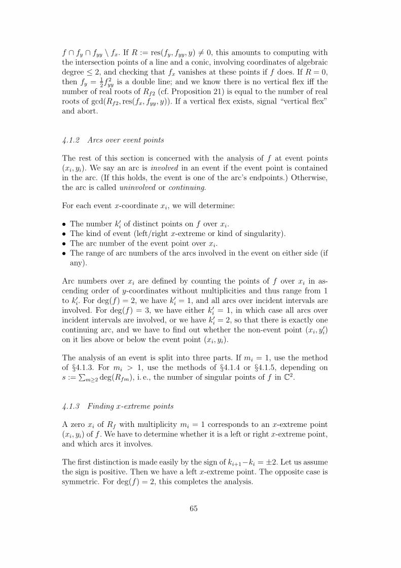
Fig. 5. The situation at interval boundaries [r−, r+] close to a left x-extreme point.

The second distinction amounts to deciding whether the uninvolved arc incase deg(f) = 3 lies above or below the x-extreme point. We use fy and fyy asauxiliary curves to make this decision. Over xi, there are two arcs of fy: onecontaining (xi, yi), because it is a double root of f(xi, y), another in between(xi, yi) and the continuing arc of f by the Mean Value Theorem. This impliesres(fy, fyy, y)(xi) 6= 0. Hence we can refine the interval ]xi, xi+1[ to an interval]r−, r+[3 ri with rational endpoints such that [r−, r+] does not contain a rootof res(fy, fyy, y).

At xi and thus over the whole interval [r−, r+], both arcs of fy lie on thesame side of the continuing arc of f . Let us compute over r− which sideit is. Between the two zeroes of fy(r−, y) lies the unique zero c of the linearpolynomial fyy(r−, y) ∈ Q[y]. Its relative position to the unique zero of f(r−, y)is determined by the sign of f(r−, c): The point (r−, c) and therefore also thex-extreme point (xi, yi) lies above/below the continuing arc of f iff f(r−, c)agrees/disagrees in sign with the leading coefficient of f .

4.1.4 Unique Singularities

Our task is to analyze a singularity (xi, yi) of f which we know to be the onlysingularity of f in C2. As we go along, we have to check the requirement that fdoes not have a vertical tangent in (xi, yi). The coordinates (xi, yi) are rational:One can read off xi ∈ Q immediately from the linear resultant factor Rfmi

.Next, yi ∈ Q can be obtained by factoring f(xi, y) ∈ Q[y] by multiplicities. Letf(x, y) = f(xi + x, yi + y). Group the terms in f = f3 + f2 by their degrees.Constant and linear part vanish since mult((0, 0); f) ≥ 2. Either f3 or f2

might also be zero. Two observations allow us to take shortcuts in computingf : The highest-order terms of f are invariant under translation. For d = 3, thequadratic part f2 can be computed by evaluating partial derivatives accordingto Taylor’s formula.

For a conic f = ay2 + bxy + cx2, the kind of singularity is all that needs to

66

be determined. Let σ = sign(b2 − 4ac). If σ > 0, then we have a crunode,involving both arcs on both sides. Else σ < 0, we have an acnode, and thereare no arcs on either side.

For a cubic, compute f(x, y) = f3(x, y) + ay2 + bxy + cx2. If a = b = c = 0,we have a triple point: It is a real triple for ki = 3 and a complex triple forki = 1, and it involves all ki = ki+1 arcs on both sides.

Otherwise, let σ = sign(b2 − 4ac) and distinguish these cases:For a = 0, signal the error “vertical singularity” and abort.For σ > 0, we have a crunode.For σ < 0, we have an acnode.For σ = 0 and |ki+1 − ki| = 2, we have a cusp.For σ = 0 and |ki+1 − ki| = 0, we have a tacnode.Factor f(0, y) = `(f)(y − y0)y

2 by setting y0 = −a/`(f).If y0 > 0, the continuing arc runs above the singularity, else it runs below.

The sign of a discriminant of a quadratic (or cubic) equation can distinguishthe cases of 0 versus 2 (or 1 versus 3) simple real roots [8, Cor. 4.19]. At variousplaces in the method above one can trade computing arc counts ki againstdetermining the sign of a discriminant. One could even exploit that for allξ ∈ R, Rf (ξ) is the discriminant of f(ξ, y) ∈ R[y] up to a constant factor anditeratively compute ki+1 from ki and mi mod 2. In terms of running time forarrangement computation, all those choices do not make a difference, becausecurve pair analyses dominate the analyses of individual curves.

4.1.5 Multiple Singularities

Assume the curve f has exactly s > 1 singular points in C2. Let exactly r ofthem be real. For r = 0 there is nothing to be done. So let (xi, yi) ∈ R2 beone of these singular points.

From §3.3, we know that deg(f) = 3 and that (xi, yi) is an acnode or crunoderesulting from the intersection of two components. By Lemma 20 we knowf(xi, y) = `(f)(y− y′

i)(y− yi)2 for some y′

i ∈ R. The required nonverticality of(xi, yi) is equivalent to yi 6= y′

i, because yi = y′i implies a threefold intersection

and hence tangency of the vertical line x − xi by Proposition 17. Thus therehas to be a non-event point (xi, y

′i) on a continuing arc of f over xi.

What we have to find out is:

• Does the nonverticality condition hold indeed?• Does the continuing arc of f run above or below (xi, yi)?• Is (xi, yi) a crunode or an acnode?

67

Let us begin with the second question. It is equivalent to computing sign(yi −y′

i). We will first construct a polynomial δ(x) ∈ Q[x] such that δ(xi) = yi − y′i.

Then we discuss its sign at xi.

Observe that the x-coordinates of all singularities of f in C2 are precisely thezeroes of the square-free polynomial h = Rf2Rf3Rf4. Let ϑ be any of them. Itis well-known how to do arithmetic in the extension field Q(ϑ) by computingin Q[x] modulo h (see §2.2.4, cf. [60]). With some care, this is possible even ifh is not irreducible. Our idea is to perform the Euclidean Algorithm for f |ϑand its derivative fy|ϑ modulo h to obtain linear factors for the double and thesimple root of f |ϑ. Dividing by fy w. r. t. y is easy since its leading coefficient isa constant. We expect the remainder to be the linear factor αy+β belonging tothe desired double root −β/α. If no choice of ϑ is a root of α, we can computea representative for 1/α modulo h by an extended gcd computation. If, on theother hand, one choice of ϑ makes α vanish, then it makes β vanish as well(because deg(gcd(f |ϑ, fy|ϑ)) = 0 is impossible), and f |ϑ has a triple root. Thismeans ϑ is the x-coordinate of a complex vertical singularity. By y-regularity,this cannot happen for a triangle, hence f is of type “conic and line” and theoffending singularity is real, violating the nonverticality condition.

Compute δ(x) as follows:Do polynomial division f = qfy + g w. r. t. y to obtain g = αy + β.Compute d, u, v ∈ Q[x] such that d = gcd(α, h) = uα + vh.If d 6= 1, signal “vertical singularity” and abort.Factor f |ϑ = `(f)ϕ1ϕ

22 by setting

ϕ2(y) := ug mod h = y + η2 and ϕ1(y) := f/(`(f)ϕ22) mod h = y + η1.

Let δ(x) = η1(x) − η2(x) ∈ Q[x].

With δ at hand, let us return to the problem of analyzing the singularity(xi, yi). If s = deg(h) = 2, then both singularities are real, we solve h for xi,and evaluate the non-zero sign of δ(xi) straight away. Since there is a real linecomponent joining the two real singularities, (xi, yi) is a crunode.

If s = 3, then f is a triangle with no vertex at infinity. Let us first consider thecase that all vertices are real and have x-coordinates x1 < x2 < x3. (All of themare crunodes.) It is obvious from the shape of a triangle that sign(δ(x1)) 6=sign(δ(x2)) 6= sign(δ(x3)). But we have deg(δ) ≤ deg(h) − 1 = 2, so thatsign(δ(x1)) = σ, sign(δ(x2)) = −σ, and sign(δ(x3)) = σ for σ := sign(`(δ)).Hence σ contains the complete answer if all vertices are real: The continuingarc runs above the singularity iff (−1)i`(δ) > 0.

In fact, the same holds if just one vertex (x1, y1) is real. (That vertex is anacnode.) For brevity, we just sketch the proof: By translating (x1, y1) to (0, 0),scaling coordinates with appropriate positive factors, and making f = ghmonic, one obtains a real line g(x, y) = y + ax + c with c = g(0, 0) 6= 0 and

68

g

f

Fig. 6. The event x-coordinates of a curve pair induce a partition of the plane intovertical lines over event x-coordinates and vertical stripes over the intervals betweenthem.

a complex line pair h(x, y) = y2 + bxy + x2 with discriminant b2 − 4 < 0.Following the construction of δ, one obtains

δ(x) =3

c(a2 − ba + 1)x2 + (4a − 2b)x + c. (17)

The factor λ(a) = a2 − ba + 1 of `(δ) has discriminant b2 − 4 < 0 and henceis positive for all a. Thus sign(`(δ)) = sign(c), where c = δ(0) is preciselythe difference of y-coordinates between the real singularity (0, 0) of f and thepoint (0,−c) on the continuing arc.

4.2 Analysis of a Pair of Cubic Curves

Let us turn to the geometric analysis of a pair {f, g} ⊆ Z[x, y] of real algebraiccurves with degrees ≤ 3. We take the same point of view as in the analysis ofone curve and ask: For a given x-coordinate ξ ∈ R, what is the number andrelative position of points of f and g over ξ, and how does this change as wevary ξ? The two-curve event points at which this changes are the one-curveevent points on either curve and the intersection points, because f ∪ g has theequation fg and the critical points

fg ∩ (fg)y = (f ∩ fy) ∪ (g ∩ gy) ∪ (f ∩ g). (18)

(This equality is easily derived from (fg)y = fyg + fgy.)

We give an algorithm that takes a pair {f, g} of algebraic curves f, g ∈ Z[x, y]of degrees ≤ 3, subject to certain conditions, and determines:

• The decomposition of the x-axis into two-curve event x-coordinates andopen intervals between them.

• The number and relative position of arcs of f and g over any ξ ∈ R.

69

• For each two-curve event: whether it is an intersection; and what kind ofone-curve event it is on f and g (if any).

• The intersection multiplicity of each intersection.• The arcs involved in each event, and the sorted sequence of arcs below and

above the event.

The conditions imposed on f and g, besides the degree bound, are as follows:

• f and g both satisfy the conditions of §4.1.• f and g are coprime.• No two points of VC(f) ∩ VC(g) are covertical.• No two event points of {f, g} are covertical.• No point of f ∩ g is an x-extreme point of f or g.• The Jacobi curve J = fxgy − fygx of {f, g} (see §4.2.4) is y-regular. For

any v ∈ R2 with mult(v; f, g) = 2 it holds that: The complex intersectionsVC(J) ∩ VC(f) and VC(J) ∩ VC(g) do not contain a point covertical to v,and the set of complex one-curve events VC(J) ∩ VC((J/ gcd(J, Jy))y) doesnot contain a point covertical or equal to v.

• If f is a complex triangle whose acnode v is a regular point of g, then fy

and g are coprime and mult(v; fy, g) is odd.

The algorithm checks these conditions and signals violations. For our goalof arrangement computation, coprimality is not a restriction, since one canreplace two curves f, g in the input to arrangement computation by h :=gcd(f, g), f/h, and g/h if h 6= 1. See §4.4 on how to establish the otherconditions.

4.2.1 Event x-Coordinates

Analogous to the analysis of one curve, the sorted sequence of two-curve eventx-coordinates induces a partition (16) of the x-axis, and again we use termslike “interval between events” and so on. The analysis of a curve pair beginsas follows.

Invoke the analysis of one curve for f and g.Compute Rfg := res(f, g, y). If Rfg = 0, signal “not coprime” and abort.Factor Rfg by multiplicities and obtain Rfg =

∏Mm=1 Rm

fgm.

Merge the real zeroes of all square-free factors of Rfg, Rf , and Rg to yieldthe sorted sequence of two-curve event x-coordinates x1 < x2 < . . . < xn andrecord their respective multiplicities m

(fg)i , m

(f)i , and m

(g)i .

If there is 1 ≤ i ≤ n such that m(fg)i = 0 ∧ m

(f)i > 0 ∧ m

(g)i > 0,

signal “covertical events” and abort.

Determine a rational sample point ri ∈]xi−1, xi[∩Q for each interval between

70

events.Find and sort the real zeroes of f(ri, y), g(ri, y) ∈ Q[y] to determine the sortedsequence of f -arcs and g-arcs over each interval between events.

Then the event points are analyzed, as detailed in the rest of this section.

4.2.2 One-curve events

Let xi be the x-coordinate of a two-curve event such that m(fg)i = 0. Then xi

originates from a one-curve event (xi, yi) on one curve, let us say f . We know(xi, yi) /∈ g, and we know g has no one-curve event over xi.

If (xi, yi) is not an isolated point of f , then its position relative to the arcs off and g can be read off directly from the position of the arcs of f containing(xi, yi) over an incident interval between events.

Now assume (xi, yi) is an isolated point of f . Such an acnode can occur on aline pair, on a singular irreducible cubic, or on a triangle. In the latter case, itcan be algebraic of degree up to 3, discouraging arithmetic with xi. However,we can use fy as an auxiliary curve that contains (xi, yi) and does not have aone-curve event at xi. If deg(fy) = 2, the Mean Value Theorem tells us thatfy has two arcs over xi, a relevant one containing (xi, yi) and another onebetween (xi, yi) and the continuing arc of f . We simply inspect the relativeposition of the relevant arc of fy and the arcs of g over a “nearby” rationalx-coordinate. “Nearby” means closer than any two-curve event of {fy, g}, i. e.,not separated from xi by a zero of res(fy, fyy, y), res(g, gy, y) or res(fy, g, y). Ifthe latter resultant is zero, fy has a common component h := gcd(fy, g) withg. But h cannot contain (xi, yi), hence we can just replace fy by fy/h andrepeat.

4.2.3 Intersections in general

Let xi be the x-coordinate of a two-curve event such that m(fg)i > 0. By the

conditions on {f, g}, there must not be an x-extreme point of f or g overxi: It may neither be covertical nor equal to the intersection point. Hence ifm

(f)i = 1 or m

(g)i = 1, we signal “x-extreme over intersection x-coordinate”

and abort. So from now on, one-curve events of f and g over xi, if any, aresingularities.

If both f and g have a singularity over xi, the situation is special insofar thatwe have explicit y-coordinates for all points from the analyses of one curveand that the noncoverticality condition requires the intersection point to beequal to both singularities. We handle this case in §4.2.7.

71

In the remaining cases, at least one of the polynomials f |xi, g|xi

∈ R[y] issquare free by Lemma 20 so that d := deg(gcd(f |xi

, g|xi)) is the number of

their distinct common complex zeroes. Hence the noncoverticality conditionfor intersection points holds iff d = 1. By Proposition 8 and y-regularity of fand g, this is equivalent to sres1(f, g, y)(xi) 6= 0. We can check this conditionwithout explicit arithmetic in xi by verifying that the gcd of the subresultantand the resultant factor defining xi has equal signs at ri and ri+1. If not, wesignal “covertical intersections” and abort. Once noncoverticality holds, theintersection multiplicity is known to be m

(fg)i .

The analysis of intersections splits into the following cases:

• Neither curve has a singularity over xi – §4.2.4.• Exactly one of the curves has a singularity over xi for which a rational

representation is known – §4.2.5.• Exactly one of the curves has a singularity over xi for which a rational

representation is not known – §4.2.6.• Both curves have a singularity over xi – §4.2.7.

The descriptions of the two asymmetric cases assume w. l. o. g. that the singu-larity is on f .

4.2.4 Intersection regular-regular

Let xi be a two-curve event x-coordinate with m := m(fg)i > 0 and m

(f)i =

m(g)i = 0. If m = 1 or after checking sres1(f, g, y)(xi) 6= 0 (cf. §4.2.3), we know

there is exactly one intersection point of f and g.

By Corollary 19, the intersection over xi causes the intersecting arcs to changesides iff m is odd. In that case, the two intersecting arcs are directly discerniblefrom the arc sequences over the incident intervals (see Figure 7(a)).

If m is even, the arc sequences over the incident intervals are equal. However,since deg(Rfg) ≤ 9 by Corollary 16, the square-free factor Rfgm defining xi

has degree at most 2 for m = 4 and degree 1 for m = 6 and m = 8, allowingus to compute explicitly with its zero xi in Q or Q(

√D), D > 0: Compute

h := gcd(f |xi, g|xi

) = y − yi, using symbolic arithmetic with√

D if necessary.Then sort the roots of f |xi

/h, g|xi/h, and h. They are pairwise distinct and

can be expressed as rationals or as one-root numbers using leda::real orCORE::Expr.

The remaining case m = 2 can be tackled using the Jacobi curve [78,79]. TheJacobi curve J of f and g is the determinant of the Jacobi matrix of the map(f, g) : R2 → R2, that is J := det(∇f, ∇g) = fxgy − fygx. The zero set of thepolynomial J consists of those points v ∈ R2 for which ∇f(v) and ∇g(v) are

72

collinear. For v ∈ f∩g this is equivalent to mult(v; f, g) ≥ 2 by Proposition 17.

Later, we need the following technical result that makes the Jacobi curvewell-defined without reference to a specific choice of coordinates.

Proposition 22 Let f, g ∈ C[x, y] be two algebraic curves and J their Jacobicurve. Let M be a linear change of coordinates. The Jacobi curve of f ◦M andg ◦M is equal to J ◦M , up to multiplication by the non-zero constant det(M).

Proof. ∇(f ◦ M) = MT((∇f) ◦ M) and det(MTN) = det(M) det(N). 2

Now we state the main theorem of [79] specialized to our case m = 2 and givea more geometric proof:

Theorem 23 Let f, g ∈ Q[x, y] be two real algebraic curves, and let v bea non-critical point of both f and g such that mult(v; f, g) = 2. Then theirJacobi curve J = fxgy − fygx is indeed a curve (i. e., non-constant) and hasintersection multiplicities mult(v; f, J) = mult(v; g, J) = 1.

Proof. Let y = α(x) and y = β(x) be the implicit functions of f and g,resp., around v. Differentiating both sides of 0 = f(x, α(x)) twice w. r. t. x,one obtains

α′(x) =−fx

fy

(x, α(x))

α′′(x) =− 1

f 3y

(fxxf

2y − 2fxyfxfy + fyyf

2x

)(x, α(x)).

Choose w. l. o. g. a scalar multiple of f such that fy < 0 around v. Then thecurvature of f at (x, α(x)) is

κf (x, α(x)) : =α′′(x)

(1 + α′(x)2)3/2=

fxxf2y − 2fxyfxfy + fyyf

2x

(f 2x + f 2

y )3/2(x, α(x))

=( 1

‖∇f‖32

(∇f⊥)T

Hf(∇f⊥))(x, α(x)), (19)

where

Hf =

fxx fxy

fxy fyy

is the Hessian matrix of f , and (a, b)⊥ = (−b, a) denotes orthogonal com-plement. By Proposition 18, mult(v; f, g) = 2 implies α′(v1) = β ′(v1) and

73

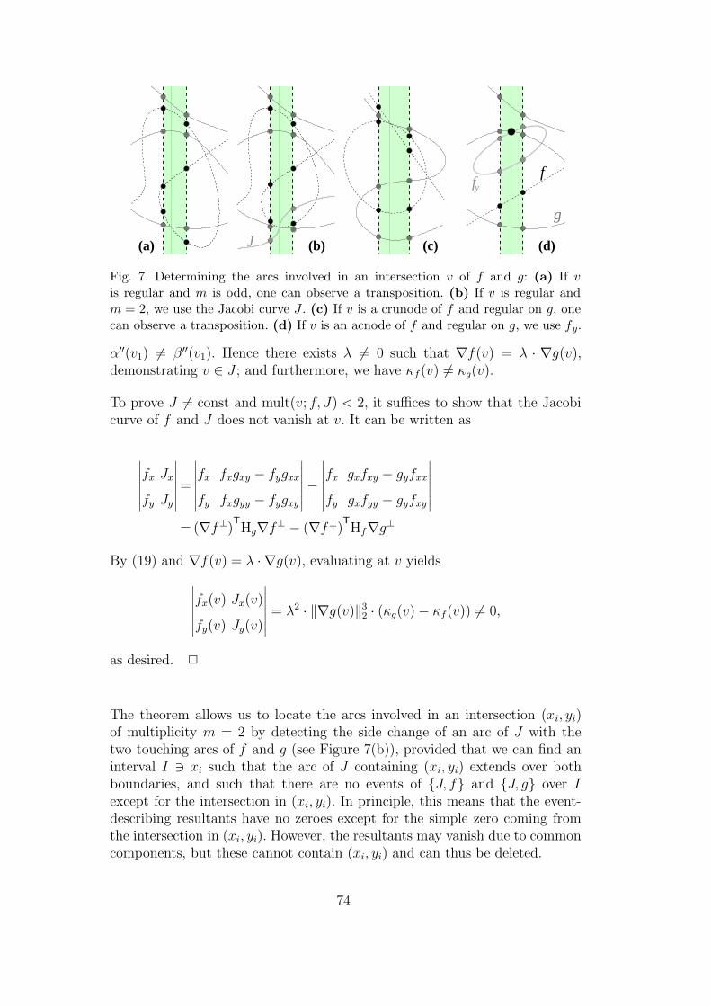
(a) (b)J (c)

fy

(d)

g

f

Fig. 7. Determining the arcs involved in an intersection v of f and g: (a) If v

is regular and m is odd, one can observe a transposition. (b) If v is regular andm = 2, we use the Jacobi curve J . (c) If v is a crunode of f and regular on g, onecan observe a transposition. (d) If v is an acnode of f and regular on g, we use fy.

α′′(v1) 6= β ′′(v1). Hence there exists λ 6= 0 such that ∇f(v) = λ · ∇g(v),demonstrating v ∈ J ; and furthermore, we have κf (v) 6= κg(v).

To prove J 6= const and mult(v; f, J) < 2, it suffices to show that the Jacobicurve of f and J does not vanish at v. It can be written as

∣∣∣∣∣∣∣

fx Jx

fy Jy

∣∣∣∣∣∣∣=

∣∣∣∣∣∣∣

fx fxgxy − fygxx

fy fxgyy − fygxy

∣∣∣∣∣∣∣−

∣∣∣∣∣∣∣

fx gxfxy − gyfxx

fy gxfyy − gyfxy

∣∣∣∣∣∣∣

= (∇f⊥)T

Hg∇f⊥ − (∇f⊥)T

Hf∇g⊥

By (19) and ∇f(v) = λ · ∇g(v), evaluating at v yields

∣∣∣∣∣∣∣

fx(v) Jx(v)

fy(v) Jy(v)

∣∣∣∣∣∣∣= λ2 · ‖∇g(v)‖3

2 · (κg(v) − κf(v)) 6= 0,

as desired. 2

The theorem allows us to locate the arcs involved in an intersection (xi, yi)of multiplicity m = 2 by detecting the side change of an arc of J with thetwo touching arcs of f and g (see Figure 7(b)), provided that we can find aninterval I 3 xi such that the arc of J containing (xi, yi) extends over bothboundaries, and such that there are no events of {J, f} and {J, g} over Iexcept for the intersection in (xi, yi). In principle, this means that the event-describing resultants have no zeroes except for the simple zero coming fromthe intersection in (xi, yi). However, the resultants may vanish due to commoncomponents, but these cannot contain (xi, yi) and can thus be deleted.

74

Our algorithm is this:Compute J := fxgy − fygx. If J is not y-regular, signal this and abort.

Let RJ := res(J, Jy, y). If RJ = 0, let J := J/ gcd(J, Jy) and repeat.Let RJf := res(J, f, y). If RJf = 0, let J := J/ gcd(J, f) and repeat.Let RJg := res(J, g, y). If RJg = 0, let J := J/ gcd(J, g) and repeat.

If xi is a zero of RJ or a multiple zero of RJf or RJg,signal “forbidden Jacobi event” and abort.

Refine the isolating interval ]ri, ri+1[ of xi to an interval [r−, r+] 3 xi containingno zero of RJRJfRJg except xi.

Compute the sorted sequences of real zeroes of f(r−, y), g(r−, y), J(r−, y) andf(r+, y), g(r+, y), J(r+, y). Compare them to detect the pair of an f -arc anda g-arc that both change sides with the same J-arc.

4.2.5 Intersection regular-singular, rational case

Let xi be a two-curve event x-coordinate with m(fg)i > 0, m

(f)i ≥ 2, and

m(g)i = 0. This means there is an intersection point of f and g, a singularity

of f , and no one-curve event of g over xi. Furthermore, let xi be known asa rational number, which is certainly the case if f has a unique singularityin C2.

Factorization of f(xi, y) ∈ Q[y] by multiplicities yields the singularity’s y-coordinate yi ∈ Q and, if present, the y-coordinate y′

i ∈ Q of a continuing arcof f . The noncoverticality condition holds iff g(xi, y

′i) 6= 0 or y′

i does not exist.If it is violated, we signal this and abort.

The continuing arcs of g correspond to zeroes of g(xi, y)/(y−yi) ∈ Q[y] whichhas degree at most 2. The sorted sequence consisting of these zeroes and yi,y′

i completely describes the geometry of {f, g} over xi.

4.2.6 Intersection regular-singular, algebraic case

Let xi be an event x-coordinate with m(fg)i > 0, m

(f)i ≥ 2, and m

(g)i = 0.

This means there is an intersection point of f and g, a singularity of f , andno event of g over xi. Assume xi is represented with defining polynomial ofdegree ≥ 2. Then the singularity of f is not unique in C2 and hence is anacnode or a crunode, according to the classification from Section 3.3.

After checking m(fg)i = 2 or sres1(f, g, y)(xi) 6= 0 (cf. §4.2.3), we know there

is exactly one intersection point of f and g over xi. It remains to check that

75

the intersection occurs in the singularity and to determine which arc of g isinvolved.

In a crunode (xi, yi) of f , two branches of f with different tangents intersect.An arc of g passing through (xi, yi) can share a tangent with at most one ofthe branches of f . Thus it changes sides with at least one of them, and weknow they change sides with each other. Therefore, a g-arc A intersects f in(xi, yi) iff one of the following conditions holds:

• On one side, A lies between the two arcs of f containing (xi, yi).• On one side, A lies below and on the other side, A lies above the respective

two arcs of f containing (xi, yi).

Hence the analysis of a crunode (xi, yi) reduces to inspecting the arc sequencesover incident intervals, see Figure 7(c) on page 74.

Let us now consider the case of an acnode (xi, yi). It occurs only for a complextriangle. The acnode has no supporting arcs on f , but we can use fy instead,similar to what we did in §4.2.2. (We described there which arc of fy contains(xi, yi).) The situation is depicted in Figure 7(d). The conic fy contains thethree non-collinear points f ∩ fy but none of their connecting lines, so it isirreducible. This entails res(fy, fyy, y) 6= 0.

We must check that the intersection of f and g over xi indeed occurs in theacnode (xi, yi) (noncoverticality), and we check that fy and g are coprimeand intersect at (xi, yi) with odd multiplicity. The latter is satisfied iff we canobserve a transposition of the relevant arc of fy with an arc of g over “nearby”rational points (where “nearby” means closer than any other event of {fy, g}),and this then is the g-arc intersecting f . So our algorithm is this:

Compute R := res(fy, g, y). If R = 0, signal “coprimality violated” and abort.If R(xi) 6= 0, signal “covertical events” and abort.

Refine ]ri, ri+1[ to ]r−, r+[ 3 xi such that [r−, r+] contains no zero of R exceptxi and no zero at all of res(fy, fyy, y).

Compare the arcs of fy and g over x = r− and x = r+:If there is a transposition of the relevant arc of fy with some arc of g,then that arc of g contains (xi, yi);else signal “no intersection in acnode visible” and abort.

4.2.7 Intersection singular-singular

Let xi be an event x-coordinate such that m(fg)i > 0, m

(f)i ≥ 2, and m

(g)i ≥ 2.

76

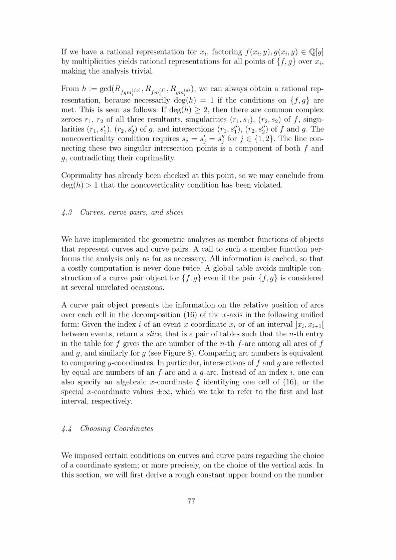
If we have a rational representation for xi, factoring f(xi, y), g(xi, y) ∈ Q[y]by multiplicities yields rational representations for all points of {f, g} over xi,making the analysis trivial.

From h := gcd(Rfgm

(fg)i

, Rfm

(f)i

, Rgm

(g)i

), we can always obtain a rational rep-

resentation, because necessarily deg(h) = 1 if the conditions on {f, g} aremet. This is seen as follows: If deg(h) ≥ 2, then there are common complexzeroes r1, r2 of all three resultants, singularities (r1, s1), (r2, s2) of f , singu-larities (r1, s

′1), (r2, s

′2) of g, and intersections (r1, s

′′1), (r2, s

′′2) of f and g. The

noncoverticality condition requires sj = s′j = s′′j for j ∈ {1, 2}. The line con-necting these two singular intersection points is a component of both f andg, contradicting their coprimality.

Coprimality has already been checked at this point, so we may conclude fromdeg(h) > 1 that the noncoverticality condition has been violated.

4.3 Curves, curve pairs, and slices

We have implemented the geometric analyses as member functions of objectsthat represent curves and curve pairs. A call to such a member function per-forms the analysis only as far as necessary. All information is cached, so thata costly computation is never done twice. A global table avoids multiple con-struction of a curve pair object for {f, g} even if the pair {f, g} is consideredat several unrelated occasions.

A curve pair object presents the information on the relative position of arcsover each cell in the decomposition (16) of the x-axis in the following unifiedform: Given the index i of an event x-coordinate xi or of an interval ]xi, xi+1[between events, return a slice, that is a pair of tables such that the n-th entryin the table for f gives the arc number of the n-th f -arc among all arcs of fand g, and similarly for g (see Figure 8). Comparing arc numbers is equivalentto comparing y-coordinates. In particular, intersections of f and g are reflectedby equal arc numbers of an f -arc and a g-arc. Instead of an index i, one canalso specify an algebraic x-coordinate ξ identifying one cell of (16), or thespecial x-coordinate values ±∞, which we take to refer to the first and lastinterval, respectively.

4.4 Choosing Coordinates

We imposed certain conditions on curves and curve pairs regarding the choiceof a coordinate system; or more precisely, on the choice of the vertical axis. Inthis section, we will first derive a rough constant upper bound on the number

77

11

1 2

2 32 3

3 4

1

2

3

3

2

1

6

5

4

3

2

1

Fig. 8. Slices of a curve pair: over an interval between events (left); over an inter-section point which is a crunode of one of the curves (right).

of forbidden directions of the y-axis per curve or curve pair. To do so, werephrase these conditions on the coordinate system as conditions that certainlines (which are well-defined without reference to a specific coordinate system)shall be non-vertical. Afterwards, we discuss how to change coordinates if acurve or curve pair analysis aborts because of a condition violation.

4.4.1 Forbidden vertical directions

Let us first consider the conditions for a single curve f . The items below matchthe items in the list of conditions given in §4.1, except for the squarefreenesscondition.

• A curve f is y-regular iff its highest-order terms are not divisible by x. Thehighest-order terms form a homogeneous polynomial of degree deg(f) whichdecomposes into linear factors over C. These are the complex asymptotes off . We obtain: f is y-regular iff none of its complex asymptotes is vertical.A cubic curve has at most 3 distinct complex asymptotes.

• No two points of VC(f) ∩ VC(fy) are covertical by Lemma 20.• A curve f has no vertical flexes iff the unique tangents in all flexes are

non-vertical. A cubic curve has at most 9 flexes [40].• The non-verticality of tangents in the singularities of a y-regular curve f ex-

cludes at most 2 further directions: For an irreducible cubic we demand thenon-verticality of the two tangents in the singularity. For a cubic consistingof a conic and a line intersecting in two distinct singularities we demandnon-verticality of the respective tangents to the conic component. A tangentto a line component is the line itself which is non-vertical by y-regularity.

This yields an upper bound of 14 on the number of forbidden directions for asingle curve.

Now consider a curve pair {f, g} and the conditions imposed in §4.2 on rela-tions between the curves, except coprimality.

• The noncoverticality of the ≤ 9 distinct complex intersection points is equiv-

78

alent to the nonverticality of the ≤(

92

)= 36 lines joining any two of them.

• The noncoverticality of intersection points to one-curve events of f is equiv-alent to the nonverticality of any line h that both contains an intersectionpoint p ∈ f ∩ g and has a multiple intersection point q 6= p with f . This isbecause a multiple intersection of h and f at q, that is mult(q; h, f) ≥ 2,means that h is a tangent to f at q or that f is singular at q (Proposition 17).

The noncoverticality of one-curve events of f and one-curve events of gis equivalent to the nonverticality of any line h that has points of multipleintersection with both f and g, by the same argument.

For both parts, we will bound the respective number of lines below, afterintroducing the necessary tools.

• There are ≤ 9 non-singular intersection points, each with a unique tangenton f and on g, respectively. These points are not extreme iff their ≤ 2·9 = 18tangents are non-vertical.

• The Jacobi curve J = fxgy − fygx is well-defined independent of a specificchoice of coordinates (Proposition 22). It has at most deg(J) ≤ 4 distinctcomplex asymptotes whose nonverticality is equivalent to y-regularity.

There are k ∈ {0, . . . , 4} non-singular intersections v of f and g withmult(v; f, g) = 2. For the noncoverticality of Jacobi intersections, no linethrough any of them that also contains another intersection of J with eitherf or g is allowed to be vertical. There are at most deg(f) deg(J)−k ≤ 12−kof those other intersections with f ; same for g. This yields ≤ 2k(12−k) ≤ 64forbidden lines.

For the absence of Jacobi one-curve events, no line through any of the≤ 4 points v that also has a multiple intersection with J is allowed to bevertical (as before because of Proposition 17). We will bound the numberof such lines below.

• Consider the acnode v of a complex triangle f . The discriminant D(x, y) ofthe quadratic part of f(x+r, y+s) is D = f 2

xy −fxxfyy by Taylor’s formula.Since v is an acnode, D(v) 6= 0. Notice that D is equal to the Jacobi curvedet(∇fy,∇fx). Hence ∇fx(v) and ∇fy(v) are linearly independent.

Partial differentiation after a change of coordinates induced by someinvertible matrix A = (aij)i,j yields the curve (((f ◦ A)y) ◦ A−1)(v) =a12fx(v) + a22fy(v) with gradient a12∇fx(v) + a22∇fy(v). Hence just onechoice of a new vertical direction (a12 : a22) makes ∇fy(v) parallel to ∇g(v);for all other choices they are non-parallel, so that coprimality of g and theirreducible conic fy as well as mult(v; fy, g) = 1 are certain.

To obtain estimates on the number of lines h fulfilling a condition of theform “h has a multiple intersection point with f (and we don’t care where)”,we lift the scene to the complex projective plane by homogenizing f(x, y) toF (x, y, z) = zdeg(f)f(x/z, y/z), and we consider the set of all complex-projec-tive lines H that have a multiple intersection point with F . Their duals H∗

form an algebraic curve F in dual space (unless F has a line component, butwe leave out this special case for brevity), which has degree deg(F )(deg(F )−1)

79

[14, pp. 252+]. For our setting, this means deg(F ) ≤ 6. (Removing the linecomponents from F , which reflect the intersections in singularities, gives thewell-known dual curve F ∗ of F [14, ibid.] [76, V.8] [40, 16.6].)

With these notions, we can now dualize “a line H through p having a multipleintersection point with curve F” to “an intersection point H∗ of line p∗ andcurve F”. This yields an upper bound deg(F ) on the number of such lines H.

Let us proceed to bound the number of lines H having a multiple intersectionwith F outside some fixed non-singular point p of F . Let T be the tangentto F at p. Recall that, for degree reasons, a line cannot have more than onemultiple intersection with a cubic. Hence “a line H through p having a multipleintersection point with curve F outside p” is equivalent to “a line H 6= Tthrough p having a multiple intersection point with curve F”. We can dualizethe latter to “an intersection point H∗ of line p∗ and curve F distinct from T ∗”.It is known [14, p. 255] that the intersection of F and p∗ at T ∗ has multiplicity2. Hence we have an upper bound of deg(F ) − 2 on the number of lines H.

Finally we can dualize “a line H having points of multiple intersection withboth F and G” to “an intersection point of F and G”. Bezout’s Theorem(p. 56) implies that no more than deg(F ) deg(G) such lines H exist.

Returning to the original question, we obtain the following bounds:

• Through each of the ≤ 9 intersection points p of f and g, there are ≤3 · 2 − 2 = 4 lines that have a multiple intersection point with f outside p;same for g. This forbids ≤ 2 · 4 · 9 = 72 directions of lines.

• There are ≤ (3 ·2)2 = 36 lines that have points of multiple intersection withboth f and g.

• Through each of the ≤ 4 non-singular intersection points of f and g withmultiplicity 2, there are ≤ 4 · 3 = 12 lines that have a multiple intersectionwith the Jacobi curve J . This forbids ≤ 4 · 12 = 48 directions of lines.

These three items forbid ≤ 72 + 36 + 48 = 156 directions. Together with the≤ 36 + 18 + 68 + 1 = 123 forbidden directions from the preceding list, weobtain that no more than 156+123 = 279 directions of a y-axis are forbiddenper analyzed curve pair.

4.4.2 Random Shearing

Since there are infinitely many possible y-axes, a random choice will pick onethat is permissible for all curves and curve pairs analyzed during the algorithmwith probability 1. Hence our strategy for finding a permissible coordinatesystem (one that is generic w. r. t. our conditions) is this: Shear the inputscene with a random shearing parameter r ∈ Q and run the algorithm. Check

80

the conditions along the way. If a violation is detected, pick a new r andrestart. A shear is an invertible linear map Sr : (x, y) 7→ (x + ry, y) for a fixedr ∈ Q. It leaves the x-axis fixed and tilts the y-axis.

From which range should the algorithm choose r? We do not recommend tocompute an a priori bound on the number of forbidden directions and definea range larger than that, because most forbidden directions will lie outsidethat range, being irrational or rational with large denominator, and choosingfrom a large range comes at a price: A value r of binary encoding length s willincrease the coefficient size of a curve f by a factor of s deg(f). Instead, startwith a small range and increase its size with the number of past failures.

4.4.3 Shearing back

We will apply curve and curve pair analyses to implement predicates forarrangement computation in Section 5. We propose to choose one globalgeneric coordinate system. Transforming input curves from the original intothe generic (sheared) system is not a problem. Analyzing curve and curvepair geometry in the sheared system has been solved above. Topological datalike the graph representing the arrangement is valid in any coordinate system.However, transforming event point coordinates back from the sheared into theoriginal coordinate system creates some complications.

Our algorithms for curve and curve pair analysis express y-coordinates in animplicit fashion as arc numbers. This entails a representation of event pointsthat is not amenable to applying the inverse shear, because there are no explicity-coordinates.

Instead, we propose to obtain approximations of coordinates: Use numericalmethods (with or without guarantees) for solving univariate polynomials to ap-proximate event point coordinates in the sheared coordinates, then transformback. Numerical approximation is made easier by the fact that the algebraiccomputations in the analysis of curves help to avoid solving for multiple zeroes.(The defining polynomials for x-coordinates ξ are explicitly made square free.The y-coordinate of a one-curve event, if not known rationally, is definablewith fy(ξ, y) instead of f(ξ, y).)

Generating correct topology and arbitrarily accurate numerical point coordi-nates is consistent with the idea of Exact Geometric Computation (EGC) [81].Using a generic coordinate system considerably reduces the number of casesdistinguished in the geometric analyses. However, there are two disadvantages:First, the sheared back result itself is not represented exactly, complicatingfurther operations on it. Second, introducing a new curve may put the for-merly generic coordinate system in violation of a position condition, requiringthe whole computation to restart with a new random choice of coordinates;

81

12 2

3

2

1

Fig. 9. Representations for a sweepable segment (left) and a point (right).

hence an incremental algorithm must retain history data to handle such anincident.

5 Arrangement Computation

We show how to perform a Bentley-Ottmann-like sweep [9] of curves, in thecomplete formulation from LEDA [62, ch. 10.7], based on the analysis of curvesand curve pairs. We emphasize that the following presentation is not restrictedto cubic curves, but works for all curves for which we can provide analysessimilar to §4.1 and §4.2 (essentially, a cylindrical algebraic decomposition withinformation on adjacencies and intersection multiplicities).

As input, we accept a set of curves. As output, our method computes a planarmap labelled with points (including auxiliary points like extreme points) andinput curves, representing the arrangement.

In a preprocessing step, every input curve f is broken into sweepable segmentssuch that each segment s has no one-curve event in its interior and such thatall points in the interior of s have the same arc number i, meaning that β isthe i-th real root of f(α, y) for every (α, β) ∈ int(s).

A segment is represented by its endpoints, its supporting curve, and its re-spective arc numbers in the interior and at the endpoints (Fig. 9 (left)). (Thisrepresentation also allows user-defined segments that are subsets of the curve’ssweepable segments.) A point is represented by an x-coordinate, a support-ing curve and an arc number (Fig. 9 (right)). To represent arcs extending toinfinity, we allow the special values −∞ and +∞ for the x-coordinate.

We outline the generalized Bentley-Ottmann algorithm for completeness (cf.Figure 10). To compute a planar map representing an arrangement of seg-ments, sweep a vertical line over them and preserve the following invariant:Left of this sweep line, the planar map has already been constructed. Thesegments intersecting the sweep line at its current position are stored in a se-quence called the Y-structure. It is sorted in ascending y-order of intersectionpoints. Right of the sweep line, all segment endpoints and some intersection

82

Y−structure

X−structure

Fig. 10. Illustration of the Bentley-Ottmann sweep line algorithm.

points – at least those of segments being adjacent in the Y-structure – arestored in a queue called the X-structure. The X-structure is sorted in lexico-graphic order.

Intersections and endpoints of segments are collectively called event points,because it is only at these points that the status of the sweep line changes.A segment containing an event point is said to be involved in the event. Theconceptual sweep over the whole plane amounts to advancing the sweep lineover this finite number of points. Covertical event points are handled in theorder of their y-coordinates; hence the lexicographic sorting of events.

The algorithm performs the following steps until the X-structure has beenemptied:

(1) Extract the next event point from the X-structure. Find the segmentsinvolved in the event by locating the event point in the Y-structure,exploiting its order.(Requires: Comparison of y-coordinates of point and segment.)

(2) Remove ending segments, i. e., those with target point equal to eventpoint.(Requires: Comparison of event point and target points.)

(3) Reorder remaining intersecting segments according to multiplicity of in-

83

tersection (explained below in §5.1) such that the new order reflects thesituation right of the event.(Requires: Segment overlap test. — Intersection multiplicity of non-over-lapping segments.)

(4) Add starting segments to the Y-structure according to its ordering.(Requires: Comparison of event point and source points. — Comparisonof segment y-order right of common point.)

(5) Add intersections of newly adjacent segments to the X-structure, obeyingits ordering.(Requires: Computation of segment intersection points. — Lexicographiccomparison of event points.)

Observe how the use of predicates by the algorithm automatically reduces allgeometric analyses to at most two curves at a time, even if many segmentsrun through one event point. 7

In summary, we need the following predicates and constructions:

Lexicographic comparison of event points. If comparing x-coordinatesdoes not break the tie, slice the two supporting curves at their commonx-coordinate to compare the supporting arcs.

Comparison of y-coordinates of point and segment. Decide this usingthe slice of the two supporting curves at the point’s x-coordinate.

Comparison of segment y-order right of common point. Inspect theslice of the two supporting curves over the interval right of the intersection.

Segment overlap test. Since different curves are required to be coprime,which is checked when the resultant of the corresponding curve pair is com-puted, segments overlap if and only if they are non-trivial, their supportingcurves are the same, their interior arc numbers are the same, and theirx-ranges overlap.

Computation of segment intersection points. Analyze the two support-ing curves over the intersection of the segments’ x-ranges. For each two-curveevent in that range, determine from the slice whether the supporting arcsof the segments coincide.

Intersection multiplicity of non-overlapping segments. This is themultiplicity of the corresponding root of res(f, g, y) by noncoverticality ofintersections.

7 Our representation of a point involves only one curve but an explicit x-coordinate,so that this view is justified, even though, for example, the comparison of twointersection points can be seen as involving four curves, i. e., the two pairs of curvescreating the intersections.

84

s1

s2

s3

s5

4s3

1

2∞

Fig. 11. Segments changing their y-order in an intersection point. The numbers onthe left are the intersection multiplicities of adjacent segments.

5.1 Reordering segments passing through an event

The reordering step (3) of the Bentley-Ottmann algorithm requires furtherexplanation, especially since this is the one place where the treatment of curvedsegments differs from the straight-line case on this level of abstraction. Wepresent the approach from [11] formalized with the notions of Section 3.

In the reordering step, depicted in Figure 11, only segments containing theevent point in their interior are involved. Let us call them s1, . . . , sk, numberedin ascending y-order just left of the event. Since the si are sweepable segments,the intersection occurs in the interior of arcs of the respective supportingcurves, and we can write a segment si locally as an analytic implicit function

y = ϕi(x) =∞∑

d=1

a(i)d xd (20)

after translating the event point to (0, 0). The coefficients of the implicit func-tions determine the y-order of segments just left and just right of the inter-section.

Proposition 24 With notation as above:Segment si lies below segment sj right of the intersection iff

(a(i)1 , a

(i)2 , . . . , a

(i)d , . . .) <lex (a

(j)1 , a

(j)2 , . . . , a

(j)d , . . .).

Segment si lies below segment sj left of the intersection iff

(−a(i)1 , a

(i)2 , . . . , (−1)da

(i)d , . . .) <lex (−a

(j)1 , a

(j)2 , . . . , (−1)da

(j)d , . . .).

(Here <lex is the lexicographic order relation on sequences of real numbers.)

Proof. It suffices to demonstrate the first part; the second part follows bysubstituting −x for x. Iff the segments overlap, they coincide around the inter-

85

section and have equal coefficient sequences. Otherwise, a finite m = min{d |a

(i)d 6= a

(j)d } exists, and ϕi(x) − ϕj(x) = (a(i)

m − a(j)m )xm + . . . is negative for

small positive x iff a(i)m < a(j)

m . 2

By Proposition 18, the quantity m considered in the proof for non-overlappingsegments is precisely the intersection multiplicity of the segments’ supportingcurves in the sense of §3.1. Incorporating the case of overlap, we define theintersection multiplicity of segments si and sj as min({d | a

(i)d 6= a

(j)d }∪{∞}).

When we come to process the intersection of s1, . . . , sk, intersection multiplic-ities will typically not have been computed for all 1

2k(k−1) pairs of segments.

For 1 ≤ i < k let mi ∈ {1, 2, 3, . . . ,∞} denote the intersection multiplicityof the adjacent segments si and si+1. These multiplicities have already beencomputed when si and si+1 were found to overlap or intersect, resp., in thecurrent event. The following result allows us to infer all other intersectionmultiplicities from them.

Proposition 25 With notation as above, the intersection multiplicity of si

and sj, 1 ≤ i < j ≤ k, is min{mi, . . . , mj−1}.

Proof. By induction on j. The base case j = i + 1 is clear. For the inductivestep from j to j+1, let m = min{mi, . . . , mj−1} be the intersection multiplicityof si and sj. For mj = ∞, the claim is clear. Otherwise, distinguish three cases:

The first case is m > mj. It holds that a(j+1)d = a

(j)d = a

(i)d for d < mj and

a(j+1)d 6= a

(j)d = a

(i)d for d = mj, so that the intersection multiplicity of si and

sj+1 is mj = min{m, mj}.

For m < mj, we have equality for d < m and inequality a(j+1)d = a

(j)d 6= a

(i)d

for d = m, demonstrating the intersection multiplicity m = min{m, mj}.

However, if m = mj, then only a double inequality a(j+1)d 6= a

(j)d 6= a

(i)d holds for

d = m, but we need a(j+1)m 6= a(i)

m . Proposition 24 helps: Since sj+1 lies above sj

and intersects with multiplicity mj = m, we know (−1)ma(j+1)m > (−1)ma(j)

m .By the analogous argument for sj and si, we know (−1)ma(j)

m > (−1)ma(i)m .

Hence (−1)ma(j+1)m > (−1)ma(i)

m , as required. 2

The proposition justifies the following way of performing step (3) (cf. [11]):

Let s1, . . . , sk be segments passing through a common event point, numberedin ascending y-order left of the event point.Let m1, . . . , mk−1 be the intersection multiplicities of adjacent segments.Let M be an even upper bound of all finite mi.

86

For m = M, M − 1, . . . , 1, take all maximal subsequences si, si+1, . . . , sj withthe property mi, mi+i, . . . , mj−1 ≥ m and reverse their order.

Observe that the intersection multiplicities mi are not readjusted to reflectthe intersection multiplicity of si and si+1 once the segments are being moved.

To prove correctness, let us first consider two non-overlapping segments, ini-tially numbered si and sj, which have been put into the same subsequenceexactly n times. This is equivalent to n = min{mi, . . . , mj−1}, since they werefirst put together for m = n and then again in every subsequent iteration. Thesegments have changed their relative position iff n is odd. By Proposition 25, nis their intersection multiplicity. By Corollary 19, the segments have to changetheir relative position iff n is odd. Hence they were rearranged correctly. Letus now consider the special case of two overlapping segments si and sj. Theybelong to a sequence of pairwise overlapping segments si, si+1, . . . , sj, so thatmi = mi+1 = . . . = mj−1 = ∞, which implies that si, sj have been put to-gether M times and have not changed their relative position (because M iseven), which is also correct.

A reader still surprised by the fact that there is no need to reorder the mi

in accordance with the permutation of segments may want to verify that thefollowing invariant holds at the beginning of a loop iteration: If mi ≤ m, thenit is the actual intersection multiplicity of si and si+1. If mi > m, then theactual intersection multiplicity is also > m.

The time complexity of segment reordering is O(M · k). In our context M isat most 10, according to Bezout’s Theorem (p. 56) and M being even.

6 Runtime Analysis

The runtime of the sweep in the Real RAM model remains the known O((n+s) log(n+m)+m) [62, ch. 10.7], where n is the number of curves, s the numberof nodes, and m the number of edges in the resulting planar map. Here it isessential that we reorder all segments passing through an intersection pointin linear time.

We consider the effect of shearing on the runtime. We show in §4.4.1 that wehave only a constant number of forbidden directions for each analyzed pair ofcurves. We conclude that a random choice among quadratically many direc-tions will lead to an expected constant number of shears. Since bit-complexityis of interest, we actually bias the choice towards directions of small bit sizerepresentations.

87

Besides the Real RAM model, the bit-complexity is of obvious importancehere. However, a complete worst-case analysis is impractical (see the numberof case distinctions), and furthermore, we expect no promising result from theknown separation bounds that we would need to apply for the (cascaded) rootisolations [19].

Instead, we emphasize that our approach is not tied to the worst case. Ourmethods benefit whenever a particular instance does not require the isolatingintervals to approach the separation bounds limit but can stop earlier. Notonly does the iteration stop earlier, e. g., in the Descartes Method, but alsothe bit complexity of the interval boundaries becomes smaller and subsequentsteps are faster. Even more important, we do not use the separation boundapproach to detect equality between our algebraic numbers. This is in contrast,e. g., to the leda::real and CORE::Expr implementations, where the equalitytest is the most costly decision. Instead we detect equality of two algebraicnumbers by finding a common factor of their defining polynomials with a rootin the appropriate interval. This is much faster than refining the intervals totheir separation bounds.

On top of this, we use modular arithmetic to quickly filter out gcd computa-tions in cases of coprime defining polynomials (§2.4.2). The same idea helpsto speed up factorization by multiplicities (§2.4.1).

In summary, we argue that the worst-case analysis of the bit complexity wouldbe non-representative for our approach. Instead, we illustrate its efficiency withthe experiments in the next section.

An alternative to the sweep-line algorithm is the randomized incremental con-struction because of its better asymptotic runtime. We can realize the neces-sary predicates with our approach. However, since we do not simply determinesigns of polynomial expressions, it is not clear whether the lower degree ofpredicates 8 for the linear case carries over to our setting.

7 Implementation and Experiments

We have implemented our method in the project Exacus, Efficient and ExactAlgorithms for Curves and Surfaces. 9

Exacus is a collection of C++ libraries;NumeriX provides the algebraic and numerical foundations, SweepX pro-vides the generic sweep-line algorithm independent of the curve type, andCubiX provides a full implementation of the curve and curve pair analyses

8 The degree of a predicate is the degree of the polynomial expression in the inputdata whose sign yields the result of the predicate.9 http://www.mpi-inf.mpg.de/projects/EXACUS/

88

of cubic curves and combines them with the sweep-line algorithm in a demoprogram. The demo visualizes curves independent of arrangement computa-tion with a subdivision method by Taubin [75] (see [61] for a survey of otheroptions). This is helpful for demonstration and debugging purposes and alsofor interactive creation of test instances.

Exacus follows the generic programming paradigm [64]. Our C++ implemen-tation is based upon design experience gained with C++ templates in thisparadigm with the Standard Template Library, Stl [7], and the Computa-tional Geometry Algorithms Library, Cgal [33,49]. One example for a genericreusable component in Exacus is the polynomial class template with the flex-ibility of different coefficient types and efficiency at the same time. More onthe software structure and design can be found in [10].

We offer three series of benchmarks. Firstly, there is a series of random sets of ncubic curves. Each curve f is defined by interpolation through 9 points chosenuniformly at random from a set of 9n random points on the {−128, . . . , 127}2

integer grid. Every interpolation point results in a homogeneous linear con-dition on the 10 unknown coefficients of f , so that generically 9 conditionsdetermine the equation of a curve uniquely, up to a constant factor. For eachinput size n, we have generated an odd number of candidate input data setsand picked the one with median average running time for inclusion in ourbenchmark.

Secondly, there is a series of degenerate instances. It is obtained in a similarfashion, except that

(1) There are only 54 interpolation points.(2) At the first interpolation point of each curve, we demand with probability

0.2 that not only f but also fx and fy vanish, making this point a rationalsingularity (yielding 2 additional linear conditions).

(3) For each interpolation point p, we pick random values for slope mp andcurvature κp. Whenever a curve f is interpolated through p, we makeits slope equal to mp (yielding one additional linear condition) and, withprobability

√0.5, we also make its curvature equal to κp (yielding a fur-

ther linear condition).

The result is an arrangement of curves with (1) vertices of high degree, (2)curves with singularities, (3) two- and threefold intersections.

Thirdly, there is a series with coefficient growth: We take the n = 60 instancesfrom the preceding random and degenerate series, scale each interpolationpoint p by a factor s = 100, 10 000, or 1 000 000, and then perturb it to sp + εwith offset vector ε chosen randomly from {−10, . . . , 10}2. (All occurrences ofan interpolation point are mapped in the same way such as to preserve degen-eracies.) This increases the bit size of the curves’ coefficients but preserves the

89

Series n segments nodes half-edges bits time

random 30 226 2933 11038 99 6.1 s

60 454 11417 44440 99 25.1 s

90 680 26579 104474 100 62.2 s

120 940 46117 181978 100 114.8 s

150 1226 71594 283114 99 180.7 s

180 1460 102298 405312 101 260.2 s

200 1554 126278 500888 101 322.5 s

degenerate 30 243 2313 8604 116 11.1 s

60 534 7627 29284 116 40.8 s

90 722 17983 70378 120 95.6 s

120 1027 31504 123814 114 168.4 s

150 1292 48362 190698 116 258.9 s

Table 1Running times in seconds for the random and degenerate benchmark instances.

combinatorial structure of the arrangement (if s is sufficiently large), allowingus to measure the increased cost of arithmetic as a function of bit sizes.

We report average running times for arrangement computations measured ona 1.2GHz Pentium IIIM system with 512 KB of cache running Linux. Theexecutable was compiled with g++ 3.1. LEDA 4.4 was used for the exact num-ber types and the internal data structures of our sweep code. All benchmarkinstances are computed in the original coordinate system; that is, they havenot been transformed with a random shear.

Table 1 reports the results for the random and degenerate instances. Eachrow states number of input curves, total number of segments after splittingof input curves, number of nodes and half-edges in the resulting graph, theaverage bit length of a curve’s longest coefficient, and the average runningtime in seconds. The running time is dominated by curve pair analyses (§4.2).The fraction of time spent on curve analyses (§4.1) is well below one secondeven for the largest instances.

The plot in Figure 12 shows the running times as a function of the number ofcomputed half-edges (output complexity). In accordance with the theoreticalanalysis, the output complexity looks almost linear. However, the output sizeis quadratic in the number of curves, as for the straight-line case.

The modular filter for gcd computations has been found to accelerate the“random 30” instance by a factor of 9. This filter and the caching of curve

90

0 60

120 180 240 300 360

100000 200000 300000 400000 500000

time

[s]

half-edges

degeneraterandom

Fig. 12. The running times from Table 1 as a function of the computed half-edges.

0 30 60 90

120 150 180 210

50 100 150 200 250 300 350 400 450 500

time

[s]

bits

degeneraterandom

Fig. 13. The running times from Table 2 as a function of average maximal coefficientlength.

and curve pair analyses for repeated use in predicate evaluations are importantsources of efficiency in our implementation.

As dominant reasons for slowdown in the degenerate instances we see: Multipleintersections of f , g cause multiple zeroes in res(f, g, y). High-degree verticescorrespond to equality of event point x-coordinates. Both phenomena entailthe computation of gcds that are avoided by the modular filter in the genericcase. The analysis of a tangential intersection requires the consideration of aJacobi curve, involving the refinement of an isolating interval against threeadditional resultants of degree 12.

Table 2 and Figure 13 show the results of the coefficient growth benchmark. Inthis setup, the increase in running time is bounded by the growth of runningtime for the exact arithmetic, especially multiplication. Our experiments usedLEDA with the O(N log2 3) Karatsuba multiplication. This superlinear growthis well-visible for the degenerate instances, and indeed they invoke more sym-bolic computations (such as gcds that are otherwise avoided and additionalresultants for Jacobi curves). For the random instances, the superlinear termis less pronounced, reflecting the fact that the coefficients of curves and resul-tants grow, whereas the interval boundaries in root isolation and comparisondo not, so that in these parts of the algorithm only one of the two operandsof multiplication grows.

Finally, we can report on a brief comparison with arrangement computation

91

Instance segments nodes half-edges bits time

random 60 454 11417 44440 99 25.1 s

with s = 102 454 11437 44520 233 47.3 s

with s = 104 454 11417 44440 361 63.8 s

with s = 106 454 11417 44440 492 84.5 s

degenerate 60 534 7627 29284 116 40.8 s

with s = 102 534 7639 29332 209 81.8 s

with s = 104 534 7627 29284 301 127.7 s

with s = 106 534 7627 29284 393 187.3 s

Table 2Running times in seconds resulting from slight perturbations that increase coefficientsizes but keep the geometry (almost) fixed.

for straight-line segments in LEDA 4.4.1. We have created sets of line segmentsdefined by pairs of points chosen randomly on the {−128, . . . , 127}2 integergrid such that the resulting arrangement has around 105 000 half-edges, similarto the “random 90” instance above. Computing such a straight-line arrange-ment using unfiltered rational arithmetic is on average about 10 times fasterthan our results for cubics. Switching on floating-point filtering accelerates thestraight-line arrangements by a further factor of 6 to 7. Recall that our codedoes not contain floating-point filtering at this time. Considering the elabo-rate algebraic methods deployed for cubics, one order of magnitude differencebetween unfiltered implementations looks quite encouraging to us.

8 Conclusion

We have reduced systematically – in theory and in the form of generic C++library code – all predicates necessary for arrangement computation of alge-braic curves to the analysis of curves and curve pairs, and to the handlingof x-coordinates. For the specific case of degree ≤ 3, we have combined tech-niques from symbolic computation with geometric observations to design andimplement these basic operations efficiently. Important parts of this design aredirectly applicable to curves of higher degree, but others – in particular in thetreatment of singularities – are not.

To achieve completeness, we choose a generic coordinate system by shearingthe input data. Although clearly useful to curb case distinctions, changingcoordinates also has its disadvantages as discussed in §4.4.3. Most notably, wecannot apply the inverse transformation on our exact implicit representation.

92

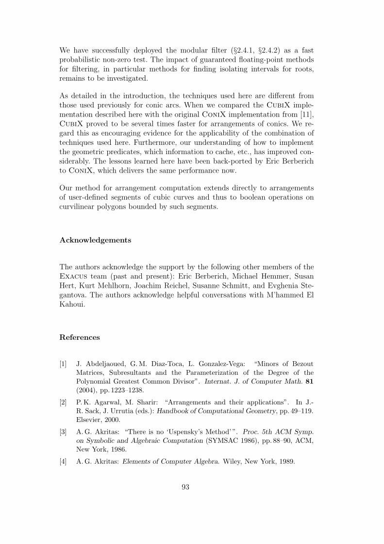
We have successfully deployed the modular filter (§2.4.1, §2.4.2) as a fastprobabilistic non-zero test. The impact of guaranteed floating-point methodsfor filtering, in particular methods for finding isolating intervals for roots,remains to be investigated.

As detailed in the introduction, the techniques used here are different fromthose used previously for conic arcs. When we compared the CubiX imple-mentation described here with the original ConiX implementation from [11],CubiX proved to be several times faster for arrangements of conics. We re-gard this as encouraging evidence for the applicability of the combination oftechniques used here. Furthermore, our understanding of how to implementthe geometric predicates, which information to cache, etc., has improved con-siderably. The lessons learned here have been back-ported by Eric Berberichto ConiX, which delivers the same performance now.

Our method for arrangement computation extends directly to arrangementsof user-defined segments of cubic curves and thus to boolean operations oncurvilinear polygons bounded by such segments.

Acknowledgements

The authors acknowledge the support by the following other members of theExacus team (past and present): Eric Berberich, Michael Hemmer, SusanHert, Kurt Mehlhorn, Joachim Reichel, Susanne Schmitt, and Evghenia Ste-gantova. The authors acknowledge helpful conversations with M’hammed ElKahoui.

References

[1] J. Abdeljaoued, G. M. Diaz-Toca, L. Gonzalez-Vega: “Minors of BezoutMatrices, Subresultants and the Parameterization of the Degree of thePolynomial Greatest Common Divisor”. Internat. J. of Computer Math. 81(2004), pp. 1223–1238.

[2] P. K. Agarwal, M. Sharir: “Arrangements and their applications”. In J.-R. Sack, J. Urrutia (eds.): Handbook of Computational Geometry, pp. 49–119.Elsevier, 2000.

[3] A.G. Akritas: “There is no ‘Uspensky’s Method’ ”. Proc. 5th ACM Symp.on Symbolic and Algebraic Computation (SYMSAC 1986), pp. 88–90, ACM,New York, 1986.

[4] A.G. Akritas: Elements of Computer Algebra. Wiley, New York, 1989.

93

[5] D. S. Arnon, G. E. Collins, S. McCallum: “Cylindrical AlgebraicDecomposition I: The Basic Algorithm”. SIAM Journal on Computing 13:4(1984) pp. 865–877.Reprinted in: B. F. Caviness, J. R. Johnson (eds.), Quantifier Elimination andCylindrical Algebraic Decomposition, pp. 136–151, Springer, 1998.

[6] D. S. Arnon, G. E. Collins, S. McCallum: “Cylindrical AlgebraicDecomposition II: An Adjacency Algorithm for the Plane”. SIAM Journalon Computing 13:4 (1984) pp. 878–889.Reprinted in: B. F. Caviness, J. R. Johnson (eds.), Quantifier Elimination andCylindrical Algebraic Decomposition, pp. 152–165, Springer, 1998.

[7] M. H. Austern: Generic Programming and the STL. Addison-Wesley, 1998.

[8] S. Basu, R. Pollack, M.-F. Roy: Algorithms in Real Algebraic Geometry.Algorithms and Computation in Mathematics, vol. 10. Springer, Berlin, 2003.See also http://www.math.gatech.edu/~saugata/bpr-posted1.html

[9] J. L. Bentley, T.A. Ottmann: “Algorithms for reporting and countinggeometric intersections”. IEEE Trans. Comput., C-28:9 (1979) pp. 643–647.

[10] E. Berberich, A. Eigenwillig, M. Hemmer, S. Hert, L. Kettner, K. Mehlhorn,J. Reichel, S. Schmitt, E. Schomer, N. Wolpert: “EXACUS: Efficient andExact Algorithms for Curves and Surfaces”. Proc. 13th European Symp. onAlgorithms (ESA 2005), pp. 155–166, Springer LNCS 3669, Berlin, 2005.

[11] E. Berberich, A. Eigenwillig, M. Hemmer, S. Hert, K. Mehlhorn, E. Schomer:“A Computational Basis for Conic Arcs and Boolean Operations on ConicPolygons”. Proc. 10th European Symp. on Algorithms (ESA 2002), pp. 174–186, Springer LNCS 2461, Berlin, 2002.

[12] P. Bikker, A. Yu. Uteshev: “On the Bezout Construction of the Resultant”.J. Symbolic Computation 28 (1999), pp. 45–88.

[13] R. Bix: Conics and Cubics: A Concrete Introduction to Algebraic Curves,Springer UTM, New York, 1998.

[14] E. Brieskorn, H. Knorrer: Plane Algebraic Curves. Birkhauser, Basel, 1986.German original: Ebene algebraische Kurven, Birkhauser, Basel, 1981.

[15] H. Bronnimann, I. Emiris, V. Pan, S. Pion: “Sign Detection in Residue NumberSystems”. Theoretical Computer Science 210 (1999), special issue on RealNumbers and Computers, pp. 173–197.

[16] W. S. Brown: “The Subresultant PRS Algorithm”. ACM Trans. Math.Software 4 (1978), pp. 237–249.

[17] W. S. Brown, J. F. Traub: “On Euclid’s Algorithm and the Theory ofSubresultants”. J. ACM 18 (1971), pp. 505–514.

[18] C. Burnikel, R. Fleischer, K. Mehlhorn, S. Schirra: “A strong and easilycomputable separation bound for arithmetic expressions involving radicals”.Algorithmica 27 (2000) pp. 87–99.

[19] C. Burnikel, S. Funke, K. Mehlhorn, S. Schirra, S. Schmitt: “A separationbound for real algebraic expressions”. Proc. 10th European Symp. onAlgorithms (ESA 2001), pp. 254–265, Springer LNCS 2161, Berlin, 2001.

94

[20] J. Canny: The Complexity of Robot Motion Planning. ACM–MIT PressDoctoral Dissertation Award Series. MIT Press, Cambridge, MA, 1987.

[21] H. Cohen: A Course in Computational Algebraic Number Theory. SpringerGTM 138, Berlin, 1993.

[22] G. E. Collins: “Subresultants and Reduced Polynomial Remainder Sequences”.J. ACM 14 (1967), pp. 128–142.

[23] G. E. Collins: “Quantifier Elimination for Real Closed Fields by CylindricalAlgebraic Decomposition”. Proc. 2nd GI Conf. on Automata Theory andFormal Languages, pp. 134–183, Springer LNCS 33, Berlin, 1975.Reprinted with corrections in: B. F. Caviness, J. R. Johnson (eds.), QuantifierElimination and Cylindrical Algebraic Decomposition, pp. 85–121, Springer,1998.

[24] G. E. Collins, A.G. Akritas: “Polynomial Real Root Isolation Using Descartes’Rule of Signs”. Proc. 3rd ACM Symp. on Symbolic and AlgebraicComputation (SYMSAC 1976), pp. 272–275, ACM, New York, 1976.

[25] D. Cox, J. Little, D. O’Shea: Ideals, Varieties, and Algorithms, 2nd ed.Springer UTM, New York, 1997.

[26] O. Devillers, A. Fronville, B. Mourrain, M. Teillaud: “Algebraic methods andarithmetic filtering for exact predicates on circle arcs”. Proc. 16th Ann. Symp.on Comp. Geom., (SCG 2000) pp. 139–147, ACM, New York, 2000.

[27] G. M. Diaz-Toca, L. Gonzalez-Vega: “Various New Expressions forSubresultants and Their Applications”. Applic. Algebra in Engin., Commun.and Computing 15 (2004), pp. 233–266.

[28] A. Eigenwillig: Exact Arrangement Computation for Cubic Curves. Master’sthesis, Saarland University, Saarbrucken, Germany, 2003.

[29] A. Eigenwillig, L. Kettner, E. Schomer, N. Wolpert: “Complete, Exact, andEfficient Computations with Cubic Curves”. Proc. 20th Ann. Symp. on Comp.Geom. (SCG 2004), pp. 409–418, ACM, New York, 2004.

[30] M. El Kahoui: “An elementary approach to subresultants theory”. J. SymbolicComputation 35 (2003), pp. 281–292.

[31] I. Emiris, A. Kakargias, S. Pion, M. Teillaud, E. Tsigaridas: “Towards anOpen Curved Kernel”. Proc. 20th Ann. Symp. on Comp. Geom. (SCG 2004),pp. 438–446, ACM, New York, 2004.

[32] I. Emiris, E. Tsigaridas: “Comparing Real Algebraic Numbers of SmallDegree”. Proc. 12th European Symp. on Algorithms (ESA 2004), pp. 652–663, Springer LNCS 3221, Berlin, 2004.

[33] A. Fabri, G.-J. Giezeman, L. Kettner, S. Schirra, S. Schonherr: “On theDesign of CGAL, a Computational Geometry Algorithms Library”. Software– Practice and Experience 30 (2000) pp. 1167–1202.

[34] E. Flato, D. Halperin, I. Hanniel, O. Nechushtan, E. Ezra: “The design andimplementation of planar maps in CGAL”. ACM J. of Exper. Algor. 5 (2000).

[35] W. Fulton: Algebraic Curves, Benjamin/Cummings, 1969. Reprint byAddison-Wesley, 1989.

95

[36] J. von zur Gathen, J. Gerhard: Modern Computer Algebra. Cambridge Univ.Press, Cambridge, 1999.

[37] J. von zur Gathen, T. Lucking: “Subresultants revisited”. TheoreticalComputer Science 297 (2003), pp. 199–239.

[38] K.O. Geddes, S.R. Czapor, G. Labahn: Algorithms for Computer Algebra.Kluwer, Norwell/Mass., 1992.

[39] I.M. Gelfand, M.M. Kapranov, A.V. Zelevinsky: Discriminants, Resultants,and Multidimensional Determinants. Birkhauser, Boston, 1994.

[40] C.G. Gibson: Elementary Geometry of Algebraic Curves: an UndergraduateIntroduction, Cambridge University Press, 1998.

[41] R.N. Goldman, T.W. Sederberg, D. C. Anderson: “Vector elimination:A technique for the implicitization, inversion, and intersection of planarparametric rational polynomial curves”. Computer Aided Geometric Design1 (1984), pp. 327–356.

[42] L. Gonzalez-Vega, I. Necula: “Efficient topology determination of implicitlydefined algebraic plane curves”. Computer Aided Geometric Design 19 (2002)pp. 719–743.

[43] D. Halperin: “Arrangements”. Chapter 24 in J. E. Goodman, J. O’Rourke(eds.): Handbook of Discrete and Computational Geometry, 2nd ed. CRCPress, Boca Raton, 2004.

[44] M. Hemmer, L. Kettner, E. Schomer: Effects of a Modular Filter on GeometricApplications. Technical Report ECG-TR-363111-01, Max-Planck-Institut furInformatik, 66123 Saarbrucken, Germany, 2004.

[45] H. Hong: “An efficient method for analyzing the topology of plane realalgebraic curves”. Mathematics and Computers in Simulation 42 (1996)pp. 571–582.

[46] X. Hou, D. Wang: “Subresultants with the Bezout Matrix”. Proceedings ofthe Fourth Asian Symp. on Computer Mathematics (ASCM 2000), pp. 19–28,World Scientific, Singapore New Jersey, 2000.

[47] J. R. Johnson: “Algorithms for Polynomial Real Root Isolation”. InB. F. Caviness, J. R. Johnson (eds.), Quantifier Elimination and CylindricalAlgebraic Decomposition, pp. 269–299, Springer, 1998.

[48] V. Karamcheti, C. Li, I. Pechtchanski, C. Yap: “A Core Library For RobustNumeric and Geometric Computation”. Proc. 15th Ann. Symp. on Comp.Geom. (SCG 1999), pp. 351–359, ACM, New York, 1999.

[49] L. Kettner, S. Naher: “Two Computational Geometry Libraries: LEDA andCGAL”. Chapter 65 in J. E. Goodman, J. O’Rourke (eds.): Handbook ofDiscrete and Computational Geometry, 2nd ed. CRC Press, Boca Raton,2004.

[50] J. Keyser, T. Culver, D. Manocha, S. Krishnan: “MAPC: A library for efficientand exact manipulation of algebraic points and curves”. Proc. 15th Ann.Symp. on Comp. Geom. (SCG 1999), pp. 360–369, ACM, New York, 1999.

[51] D. E. Knuth: The Art of Computer Programming, vol. 2: SeminumericalAlgorithms, 3rd ed. Addison-Wesley, 1998.

96

[52] W. Krandick: “Isolierung reeller Nullstellen von Polynomen”. In: J. Herzberger(ed.), Wissenschaftliches Rechnen, pp. 105–154, Akademie-Verlag, Berlin,1995.

[53] W. Krandick, K. Mehlhorn: “New Bounds for the Descartes Method”.Tech. Rep. DU-CS-04-04, Drexel University, Dept. of Computer Science,http://www.cs.drexel.edu/static/reports/DU-CS-04-04.html

To appear in J. Symbolic Computation.

[54] S. Lang: Algebra, 2nd ed. Addison-Wesley, 1984.

[55] C. Li, C. Yap: “A New Constructive Root Bound for Algebraic Expressions”.Proc. 12th ACM-SIAM Symp. on Discrete Algorithms (SODA 2001), pp. 496–505, ACM, New York, 2001.

[56] T. Lickteig, M.-F. Roy: “Cauchy Index Computation”. Calcolo 33 (1996),pp. 337–351.

[57] T. Lickteig, M.-F. Roy: “Sylvester-Habicht Sequences and Fast Cauchy IndexComputation”. J. Symbolic Computation 31 (2001), pp. 315–341.

[58] H. Lombardi, M.-F. Roy, M. Safey El Din: “New Structure Theorem forSubresultants”. J. Symbolic Computation 29 (2000), pp. 663–689.

[59] R. Loos: “Generalized Polynomial Remainder Sequences”. In B. Buchbergeret al. (eds.): Computer Algebra. Symbolic and Algebraic Computation, 2nded., pp. 115–137. Springer, Wien, 1983.

[60] R. Loos: “Computing in Algebraic Extensions”. In B. Buchberger et al. (eds.):Computer Algebra. Symbolic and Algebraic Computation, 2nd ed., pp. 173–187. Springer, Wien, 1983.

[61] R. Martin, H. Shou, I. Voiculescu, A. Bowyer, G. Wang: “Comparison ofInterval Methods for Plotting Algebraic Curves”. Computer Aided GeometricDesign 19:7 (2002), pp. 553–587.

[62] K. Mehlhorn, S. Naher: LEDA: A platform for combinatorial and geometriccomputing. Cambridge Univ. Press, Cambridge, 1999.

[63] M. Mignotte: Mathematics for Computer Algebra. Springer, 1992.

[64] D. R. Musser, A. A. Stepanov: “Algorithm-oriented Generic Libraries”.Software – Practice and Experience 24 (1994) pp. 623–642.

[65] A.M. Ostrowski: “Note on Vincent’s Theorem”. Annals of Mathematics,Second Series, 52 (1950), pp. 702–707, 1950.Reprinted in: A. Ostrowski, Collected Mathematical Papers, vol. 1, pp. 728–733, Birkhauser, 1983.

[66] P. Pedersen: “Multivariate Sturm Theory”. Proc. 9th Int. Symp. Appl.Algebra, Algeb. Algor. and Error-Corr. Codes (AAECC-9), pp. 318–332,Springer LNCS 539, 1991.

[67] F. P. Preparata, M. I. Shamos: Computational Geometry: An Introduction.Springer, New York, 1985.

[68] G. Rote: “Division-free algorithms for the determinant and the Pfaffian”.In H. Alt (ed.), Computational Discrete Mathematics, pp. 119–135, SpringerLNCS 2122, Berlin, 2001.

97

[69] F. Rouillier, P. Zimmermann: “Efficient isolation of polynomial’s real roots”.J. Computational and Applied Math. 162 (2004), pp. 33–50.

[70] T. Sakkalis, R. Farouki: “Singular Points of Algebraic Curves”. J. SymbolicComputation 9 (1990), pp. 405–421.

[71] T. Sakkalis: “The topological configuration of a real algebraic curve”. Bulletinof the Australian Mathematical Society 43 (1991) pp. 37–50.

[72] S. Schmitt: “The diamond operator: Implementation of exact real algebraicnumbers”. Proc. 8th Internat. Workshop on Computer Algebra in Scient.Comput. (CASC 2005), pp. 355–366, Springer LNCS 3718, Berlin, 2005.

[73] E. Schomer, N. Wolpert: “An Exact and Efficient Approach for Computinga Cell in an Arrangement of Quadrics”. Computational Geometry 33 (2006)pp. 65–97.

[74] M. Seel: Implementation of planar Nef polyhedra. Report MPI-I-2001-1-003,Max-Planck-Institut fur Informatik, 66123 Saarbrucken, Germany, 2001.

[75] G. Taubin: “Rasterizing Algebraic Curves and Surfaces”. IEEE ComputerGraphics and Applications 14 (1994), pp. 14–23.

[76] R. J. Walker: Algebraic Curves. Princeton University Press, 1950.

[77] R. Wein: “High-level filtering for arrangements of conic arcs”. Proc. 10thEuropean Symp. on Algorithms (ESA 2002), pp. 884–895, Springer LNCS2461, Berlin, 2002.

[78] N. Wolpert: An Exact and Efficient Approach for Computing a Cell in anArrangement of Quadrics. Ph.D. thesis, Saarland University, Saarbrucken,Germany, 2002.

[79] N. Wolpert: “Jacobi Curves: Computing the Exact Topology of Arrangementsof Non-Singular Algebraic Curves”. Proc. 11th European Symp. on Algorithms(ESA 2003), pp. 532–543, Springer LNCS 2832, Berlin, 2003.

[80] C.K. Yap: Fundamental Problems of Algorithmic Algebra. Oxford UniversityPress, New York, 2000.

[81] C.K. Yap: “Robust Geometric Computation”. Chapter 41 in: J. E. Goodman,J. O’Rourke (eds.): Handbook of Discrete and Computational Geometry, 2nded. CRC Press, Boca Raton, 2004.

[82] C.K. Yap: “Complete Subdivision Algorithms, I: Intersection of BezierCurves”, extended abstract.ftp://cs.nyu.edu/pub/local/yap/exact/bezier1.ps.gz

98