Experimental analysis on membrane wrinkling under

biaxial load - Comparison with bifurcation analysis

Yann Lecieux, Rabah Bouzidi

To cite this version:

Yann Lecieux, Rabah Bouzidi. Experimental analysis on membrane wrinkling under biaxialload - Comparison with bifurcation analysis. International Journal of Solids and Structures,Elsevier, 2010, 47 (18 19), pp.2459-2475. <10.1016/j.ijsolstr.2010.05.005>. <hal-01006831>

HAL Id: hal-01006831

https://hal.archives-ouvertes.fr/hal-01006831

Submitted on 3 Dec 2016

HAL is a multi-disciplinary open accessarchive for the deposit and dissemination of sci-entific research documents, whether they are pub-lished or not. The documents may come fromteaching and research institutions in France orabroad, or from public or private research centers.

L’archive ouverte pluridisciplinaire HAL, estdestinee au depot et a la diffusion de documentsscientifiques de niveau recherche, publies ou non,emanant des etablissements d’enseignement et derecherche francais ou etrangers, des laboratoirespublics ou prives.

Distributed under a Creative Commons Attribution 4.0 International License

1

Experimental analysis on membrane wrinkling under biaxial load – Comparisonwith bifurcation analysis

Y. Lecieux, R. BouzidiNantes University, Institute in Civil and Mechanical Engineering (GeM), UMR 6183, Faculté des Sciences et des Techniques, 2 rue de la Houssinière, Nantes F-44000, France

ental ne ten

wrink

enomeducibilque wrxperim

This paper presents a detailed experimmembranes under the action of in-plaaxes using various loading paths. Theanalysis method. Over this experiment, several phon the wrinkle pattern, and the repro The main result is that non-uniconditions. The uncertainty of the efinite element analysis.

Keywords: Membrane, Gossamer structures, Field mea

imental surveys exist regarding fine detakling. Indeed, for such compliant materiawrinkle shape must be made using a non

study of the formation and evolution of the wrinkle pattern that form in flat elastic and isotropic sion. The experiments were carried out on a cruciform specimen stretched along two uncoupled led shapes of the membrane were digitized by using a full-field measurement based on the fringe

na were observed: the mechanism of wrinkle division, the influ-ence of the membrane thickness ity of a kinematic configuration of wrinkles.inkle shapes have been observed over repeated experiments for nominally identical boundary ental wrinkle shape has been explained using comparison with the results of a post-buckling

sure, Fringe analysis, Bifurcation analysis, Buckling

1. Introduction

Over the past 20 years there have been a large number of newstructural concepts for large spacecraft applications involvingstretched membrane surfaces (Jenkins, 2001). Compared to tradi-tional spacecraft structures, the ‘‘Gossamer structures” could pro-vide many advantages such as reduced mass and volume.Gossamer structures are designed for such applications as anten-nas, solar arrays and telescope lenses. However, the membranesused in gossamer structures cannot undergo compressive stressbecause of their small bending stiffness. The result of compressivestress is that buckling occurs leading to membrane wrinkling. Thismay affect the performance and the reliability of the flexible gossa-mer structures (as in the case of antennas or reflectors). Thus, theprediction of wrinkle patterns in membrane surfaces is one of themany current technological interests in the aerospace industry.

This paper presents a detailed experimental study of the forma-tion and evolution of the wrinkle patterns that form in flat isotro-pic membranes. The experiments were carried out on cruciformspecimens stretched under in-plane uncoupled biaxial loads. Theanalysis of membrane wrinkling has a long history which startedwith the works of Wagner (1929). Nevertheless, only recent exper-

ils of membrane wrin-l, the measure of the

-contact method. Since

the works of Jenkins et al. (1998) several authors have taken inter-est in the study of wrinkle details and its evolution (Cerda et al.,2002; Wong and Pellegrino, 2006a; Wang et al., 2009). In the pres-ent work, results are presented for two uncoupled loading param-eters allowing various loading paths while the above mentionedpapers deal with the effect of a single loading parameter. The studystarts with the presentation of detailed results such as the shape,the amplitude and the wavelength of wrinkles. These data consti-tute a valuable experimental database for the validation of numer-ical procedures of wrinkling simulation.

The particular purpose of this work is the observation of thereproducibility of the wrinkle patterns that form on the surfaceof different specimens for nominally identical boundary condi-tions. The main result is that non-unique wrinkle shapes have beenobserved over repeated experiments. These different experimentalwrinkle shapes have been reproduced in accordance with thebifurcation theory using a post-buckling finite element analysis.

Experiments performed on a cruciform test specimen are pre-sented in this paper. In each experiment, the whole 3D shape ofthe membrane has been digitized using a non-contact measure-ment method: the fringe analysis. The mechanism of wrinkle divi-sion has been observed and explained. Wrinkle details forspecimens of various thicknesses including the number, amplitudeand wavelength of the wrinkles are given here. Then the uncer-tainty of the wrinkle shape is discussed.

The paper is organized as follows: Section 2 presents a review ofprevious experimental and numerical works on the topic of thinelastic membrane wrinkling. Section 3 describes the experimental

2

materials and methods. Experimental results are presented in Sec-tion 4 and analyzed in Section 5. In Section 6 the finite elementprocedure of wrinkling simulation is described and comparison ismade between experimental and numerical results. Then Section7 concludes the paper.

2. Review of previous works

2.1. Review of experimental measurement of wrinkling

The first survey regarding the wrinkling experiment is attributedto Wagner (1929). He studied the formation of localized buckling inthin metal structures used in the aircraft industry. Later, in the1960s, NASA developed gossamer structures. The main outcomewas the launch of the echo balloon series. At that time, (Stein andHedgepeth, 1961) offered a theory to analyze partly wrinkled mem-branes. They carried out an experiment on a flat stretched mem-brane wrinkled by rotation of a central hub. This study was builtupon by the works of Mikulas (1964). More recently, Miyamura(2000) used strain gauges to study the stress distribution in similarstructure. He ran experimental results against those obtainedthrough a numerical analysis. Another well-known problem is theshearing of an initially flat rectangular membrane as proposed byMansfield (1970). He observed the wrinkle orientation on shearingpanels in different configurations. However, due to the impossibilityof using non-contact methods to measure the out-of-plane displace-ment, the authors cited above (except for Miyamura on stressmeasurement) only made qualitative correlations between theirexperiments and their theoretical results.

Jenkins was the first to provide accurate measurements of wrin-kle details. He studied a rectangular panel under shear stress (Jen-kins et al., 1998) using a capacitance sensor. Nevertheless, thesensor he used limits the applications to metallic surfaces. Wongand Pellegrino (2006a) carried out two sets of experiments: a rectan-gular membrane under simple shear, and a square membrane sub-jected to two pairs of equal and opposite diagonal forces. Themeasurement of wrinkle details was performed using a laser dis-placement sensor. This sensor, like the capacitance sensor, doesnot enable to observe the deflection of the whole membrane, andonly cross-sections are measurable.

The use of the photogrammetry method proposed by Blandinoenabled the observation of the whole specimen surface. This tech-nique was used to study the effect of symmetric or asymmetricmechanical and thermal loading on membrane wrinkling (Blandinoet al., 2001, 2002a,b). The same technique has recently been used byWang et al. (2009) to study a square membrane in tension. In thisexperiment, the non-uniform distribution of stress during the appli-cation of the tensile loads leads to membrane wrinkling.

2.2. Review of numerical procedures of wrinkling simulation

The analysis of the wrinkling behavior of membrane structuresstarted with the works of Wagner (1929), who initiated the meth-od called Iterative Material Procedures (IMP). This method takeinto account only the in-plane stiffness. The bending stiffness isnot evaluated. These wrinkling models are mainly based on themodification of the deformation gradient or of the constitutiveequation in order to avoid compressive stresses (Kang and Im,1997; Epstein and Forcinito, 2001). As a result, this kind of ap-proach does not make it possible to represent wrinkle patternsand does not provide any information about the size of wrinkles.This aspect is a major disadvantage of the membrane model. How-ever, the stress field and wrinkling zone are correctly determined.Mansfield (1968) and Pipkin (1986) reformulated the theory byusing a suitable relaxed energy density as defined in the Tension

Field Theory. The relaxed energy density represents the averageenergy per initial area unit over a region containing many wrinkles.

The most adequate method to accurately predict the wrinkle pat-terns is the use of an extensively refined mesh with thin-shell ele-ments possessing bending stiffness. This approach enables toprecisely analyze the buckling and post-buckling response of themembrane under tension. Its detailed developments can be foundin Riks (1979) and Crisfield (1997). It involves a geometrical non-lin-ear eigenvalue analysis and leads to the most realistic solution.However, heavy computations are implied due to the dense mesh.A wrinkling analysis, using the buckling of shell element, is typicallyperformed in three stages: The first consists in obtaining a stable ini-tial state in the case of very thin shells. This is often achieved byapplying slight initial pre-stress that increased the low bending stiff-ness of thin shells by the geometrical bending stiffness. The secondstep is an eigenvalue buckling analysis which gives the mode shapesof the membrane. Mode shapes are introduced as geometricalimperfections in the third step of the post-buckling analysis.

3. Experimental program

The aim of this experimental study is to provide a means tocharacterize the phenomenon of wrinkling for membranes sub-jected to in-plane loads. The formation and evolution of wrinklesare studied on cruciform specimens. They are tested on biaxialapparatus with various loading paths. The tests are conducted byprescribing displacement in symmetrical way along two orthogo-nal axes. During the tests, the displacement of each clamped edgeas well as the imposed force are measured. To get complete exper-imental data, the out-of-plane displacement of the tested mem-brane is also digitized using an optical method of fringe projection.

Additionally, the influence of membrane thickness on wrinklepatterns is considered, as well as the reproducibility of kinematicconfigurations when several quasi-identical specimens – in termsof material, dimensions and thickness – are submitted to a samegiven load path. To this end, three identical specimens were testedfor each experimental condition. Finally, experiments were per-formed on nine specimens – with three specimens for each ofthe three different thicknesses considered.

3.1. Biaxial testing apparatus

The biaxial tests were carried out using a particular and dedi-cated biaxial testing apparatus equipped with two orthogonal,independent, and symmetrical loading axes (see Fig. 1). Along eachloading direction, the displacement is applied on the specimen by apair of cross-bars sliding symmetrically along two parallel guiderails. The displacements of the cross-bars are prescribed manuallyfor each axis thanks to a precision screw, which maintains them atan equal distance from the centre of the device. Each cross-bar isequipped with a displacement probe and a load cell rated 10 kN.Measurement were performed using a displacement sensor witha linearity of 0.2% of full scale and a maximum range of 25 mm.

3.2. Specimens

The biaxial tests were performed on cruciform specimensaccording to the geometry depicted in Fig. 2.

The membrane tested is the Kapton� VN polyimide film, usedfor spacecraft applications. Table 1 (DuPont, 2006) summarizesthe material characteristics of the specimens.

3.3. Test procedure

The steps of the experimental protocol performed on the spec-imens presented in Table 1 include the positioning of the

Fig. 1. Biaxial testing machine.

Fig. 2. Geometry of the tested specimens.

Table 1Material characteristics of tested membranes.

Thickness(lm)

Number of testspecimens

Type ofKapton

Young modulus(MPa)

Poissonratio

125 3 VN 2800 0.3450 3 VN 2800 0.3425 3 VN 2800 0.34

Table 2Preloading counterweight values.

Thickness (lm) Total value of counterweight (g)

125 100050 40025 200

Fig. 3. Positioning of the membrane.

Table 3Prescribed displacement paths.

Load path i

d1 (mm) d2 (mm)

�[0.5 � (i � 1)] 0�[0.5 � (i � 1)] 0.5�[0.5 � (i � 1)] 1.0�[0.5 � (i � 1)] 1.5�[0.5 � (i � 1)] 2.0�[0.5 � (i � 1)] 2.5�[0.5 � (i � 1)] 3.0

3

membrane on the apparatus, then the application of a small initialstress to its four edges before clamping the membrane to the fourcross-bars. Finally, the desired displacement paths are applied.

During membrane installation, the biaxial testing machine isplaced in horizontal position. A slight initial tension is applied tothe membrane by means of counterweight connected throughcords running over pulleys via aluminum rigid blocks glued to

the four edges of the specimen. A similar system was used in thestudy of Wong and Pellegrino (2006a). The total value of the coun-terweight applied on one edge is given in Table 2.

These preloading values guarantee identical stress field for thethree thicknesses and hence a quasi plane shape for the membrane.The membrane is then clamped to the cross-bars. The different ele-ments described above are shown in Fig. 3.

After clamping the specimen, various displacement paths areapplied to the cross-bars. Table 3 summarizes the applied paths(with i = 1 ? 7).

For each prescribed displacement, the acquired data are the in-plane displacements, the loads applied on the edges of the speci-men, and also the out-of-plane displacements of the membranecaused by the wrinkling phenomenon.

3.4. Measure of the out-of-plane displacement

To measure the shape of the wrinkles, the technique called‘‘Fringe projection method” was used, see Robinson and Reid(1993) and Yoshizawa (2009). It is based on the analysis of thedeformation of fringes projected onto the studied object, whichacts as a screen. The fringes are projected thanks to a standard vi-deo projector. It is a full-field and non-contact method which pro-vides the deflection z of every point of the deformed surface.During the test, images of cruciform specimens are recorded foreach loading step using a CCD camera. For each displacement step,this method allowed the digitization of the 3D shape of the wholemembrane.

4

3.5. Fringe deformation method

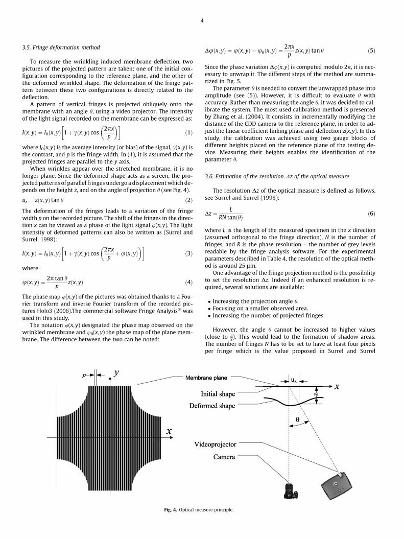
To measure the wrinkling induced membrane deflection, twopictures of the projected pattern are taken: one of the initial con-figuration corresponding to the reference plane, and the other ofthe deformed wrinkled shape. The deformation of the fringe pat-tern between these two configurations is directly related to thedeflection.

A pattern of vertical fringes is projected obliquely onto themembrane with an angle h, using a video projector. The intensityof the light signal recorded on the membrane can be expressed as:

Iðx; yÞ ¼ I0ðx; yÞ 1þ cðx; yÞ cos2px

p

� �� �ð1Þ

where I0(x,y) is the average intensity (or bias) of the signal, c(x,y) isthe contrast, and p is the fringe width. In (1), it is assumed that theprojected fringes are parallel to the y axis.

When wrinkles appear over the stretched membrane, it is nolonger plane. Since the deformed shape acts as a screen, the pro-jected patterns of parallel fringes undergo a displacement which de-pends on the height z, and on the angle of projection h (see Fig. 4).

ux ¼ zðx; yÞ tan h ð2Þ

The deformation of the fringes leads to a variation of the fringewidth p on the recorded picture. The shift of the fringes in the direc-tion x can be viewed as a phase of the light signal u(x,y). The lightintensity of deformed patterns can also be written as (Surrel andSurrel, 1998):

Iðx; yÞ ¼ I0ðx; yÞ 1þ cðx; yÞ cos2px

pþuðx; yÞ

� �� �ð3Þ

where

uðx; yÞ ¼ 2p tan hp

zðx; yÞ ð4Þ

The phase map u(x,y) of the pictures was obtained thanks to a Fou-rier transform and inverse Fourier transform of the recorded pic-tures Holo3 (2006).The commercial software Fringe Analysis� wasused in this study.

The notation u(x,y) designated the phase map observed on thewrinkled membrane and u0(x,y) the phase map of the plane mem-brane. The difference between the two can be noted:

Fig. 4. Optical mea

Duðx; yÞ ¼ uðx; yÞ �u0ðx; yÞ ¼2px

pzðx; yÞ tan h ð5Þ

Since the phase variation Du(x,y) is computed modulo 2p, it is nec-essary to unwrap it. The different steps of the method are summa-rized in Fig. 5.

The parameter h is needed to convert the unwrapped phase intoamplitude (see (5)). However, it is difficult to evaluate h withaccuracy. Rather than measuring the angle h, it was decided to cal-ibrate the system. The most used calibration method is presentedby Zhang et al. (2004). It consists in incrementally modifying thedistance of the CDD camera to the reference plane, in order to ad-just the linear coefficient linking phase and deflection z(x,y). In thisstudy, the calibration was achieved using two gauge blocks ofdifferent heights placed on the reference plane of the testing de-vice. Measuring their heights enables the identification of theparameter h.

3.6. Estimation of the resolution Dz of the optical measure

The resolution Dz of the optical measure is defined as follows,see Surrel and Surrel (1998):

Dz ¼ LRN tanðhÞ ð6Þ

where L is the length of the measured specimen in the x direction(assumed orthogonal to the fringe direction), N is the number offringes, and R is the phase resolution – the number of grey levelsreadable by the fringe analysis software. For the experimentalparameters described in Table 4, the resolution of the optical meth-od is around 25 lm.

One advantage of the fringe projection method is the possibilityto set the resolution Dz. Indeed if an enhanced resolution is re-quired, several solutions are available:

� Increasing the projection angle h.� Focusing on a smaller observed area.� Increasing the number of projected fringes.

However, the angle h cannot be increased to higher values(close to p

2). This would lead to the formation of shadow areas.The number of fringes N has to be set to have at least four pixelsper fringe which is the value proposed in Surrel and Surrel

sure principle.

Fig. 5. Principle of picture analysis as used in the fringe projection method.

Table 4Experimental parameters for the optical measure.

Angle of projection h(deg) 40Number of pixels 4500 � 3000Number of fringes N 280Phase resolution R 100Length of observed shape L (mm) 600

5

(1998). In this experiment, the number of pixels is about 12 perfringe.

4. Experimental results

This section presents detailed experimental results on the evo-lution of the shape of wrinkles under load. In particular, the mech-anism of wrinkle division is explained. Then, the reproducibility ofthe kinematic configurations of the wrinkles is discussed.

Fig. 6. Sample of experimental out-of-plane displacements (specimenthickness = 50 lm).

4.1. Wrinkle patterns

The typical wrinkle pattern of a deformed membrane (seeFig. 6) shows a double symmetric shape with three main regionsof instability. There are slack zones near the circular edges of themembrane. In the middle area, the presence of primary wrinklesparallel to the direction of the tension loading, axis y is visible. Fi-nally, there are transition zones between the primary wrinkles andthe slack zones. These are called secondary wrinkling zones byanalogy with the work of Wang et al. (2009).

The wrinkle represented in the above pattern is generic. Morespecifically, the presence of slack zones and secondary wrinklesdepends on the loading path. Photographic samples of the mem-brane shape for different prescribed displacements are shown inFig. 7.

This pictorial matrix shows widely varying geometrical config-urations of wrinkles. This is due to the control of the applied dis-placement with two independent parameters. Here, the seven

loading paths studied for each of the nine test specimens formeda really consequent experimental database. Indeed, each loadingpath constitutes a possible validation case for numerical proce-dures of wrinkling simulation.

4.2. Modification of shape under load

Wrinkle details and their formation mechanisms are furtherinvestigated by plotting three cross-sections of the tested speci-mens, in particular by plotting the out-of-plane displacement zagainst the x axis at different values of y. Fig. 8b and c shows sam-ples of the obtained cross-sections for a given load step(d1 = �0.5 mm and d2 = 3 mm). The central section, (y = 0), givesuseful characteristics of primary wrinkling while sections at

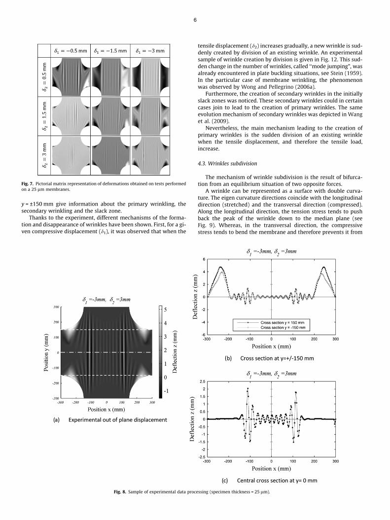
Fig. 7. Pictorial matrix representation of deformations obtained on tests performedon a 25 lm membranes.

6

y = ±150 mm give information about the primary wrinkling, thesecondary wrinkling and the slack zone.

Thanks to the experiment, different mechanisms of the forma-tion and disappearance of wrinkles have been shown. First, for a gi-ven compressive displacement (d1), it was observed that when the

Fig. 8. Sample of experimental data proce

tensile displacement (d2) increases gradually, a new wrinkle is sud-denly created by division of an existing wrinkle. An experimentalsample of wrinkle creation by division is given in Fig. 12. This sud-den change in the number of wrinkles, called ‘‘mode jumping”, wasalready encountered in plate buckling situations, see Stein (1959).In the particular case of membrane wrinkling, the phenomenonwas observed by Wong and Pellegrino (2006a).

Furthermore, the creation of secondary wrinkles in the initiallyslack zones was noticed. These secondary wrinkles could in certaincases join to lead to the creation of primary wrinkles. The sameevolution mechanism of secondary wrinkles was depicted in Wanget al. (2009).

Nevertheless, the main mechanism leading to the creation ofprimary wrinkles is the sudden division of an existing wrinklewhen the tensile displacement, and therefore the tensile load,increase.

4.3. Wrinkles subdivision

The mechanism of wrinkle subdivision is the result of bifurca-tion from an equilibrium situation of two opposite forces.

A wrinkle can be represented as a surface with double curva-ture. The eigen curvature directions coincide with the longitudinaldirection (stretched) and the transversal direction (compressed).Along the longitudinal direction, the tension stress tends to pushback the peak of the wrinkle down to the median plane (seeFig. 9). Whereas, in the transversal direction, the compressivestress tends to bend the membrane and therefore prevents it from

ssing (specimen thickness = 25 lm).

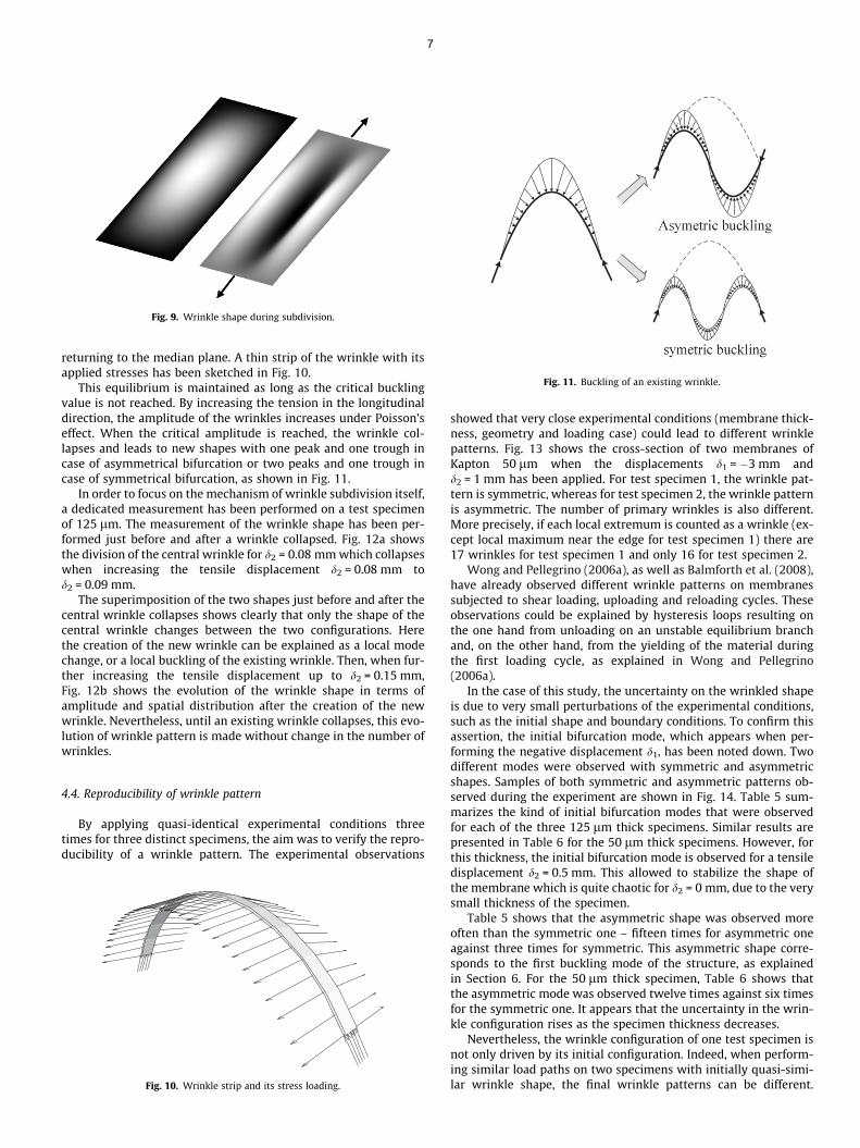
Fig. 9. Wrinkle shape during subdivision.

Fig. 11. Buckling of an existing wrinkle.

7

returning to the median plane. A thin strip of the wrinkle with itsapplied stresses has been sketched in Fig. 10.

This equilibrium is maintained as long as the critical bucklingvalue is not reached. By increasing the tension in the longitudinaldirection, the amplitude of the wrinkles increases under Poisson’seffect. When the critical amplitude is reached, the wrinkle col-lapses and leads to new shapes with one peak and one trough incase of asymmetrical bifurcation or two peaks and one trough incase of symmetrical bifurcation, as shown in Fig. 11.

In order to focus on the mechanism of wrinkle subdivision itself,a dedicated measurement has been performed on a test specimenof 125 lm. The measurement of the wrinkle shape has been per-formed just before and after a wrinkle collapsed. Fig. 12a showsthe division of the central wrinkle for d2 = 0.08 mm which collapseswhen increasing the tensile displacement d2 = 0.08 mm tod2 = 0.09 mm.

The superimposition of the two shapes just before and after thecentral wrinkle collapses shows clearly that only the shape of thecentral wrinkle changes between the two configurations. Herethe creation of the new wrinkle can be explained as a local modechange, or a local buckling of the existing wrinkle. Then, when fur-ther increasing the tensile displacement up to d2 = 0.15 mm,Fig. 12b shows the evolution of the wrinkle shape in terms ofamplitude and spatial distribution after the creation of the newwrinkle. Nevertheless, until an existing wrinkle collapses, this evo-lution of wrinkle pattern is made without change in the number ofwrinkles.

4.4. Reproducibility of wrinkle pattern

By applying quasi-identical experimental conditions threetimes for three distinct specimens, the aim was to verify the repro-ducibility of a wrinkle pattern. The experimental observations

Fig. 10. Wrinkle strip and its stress loading.

showed that very close experimental conditions (membrane thick-ness, geometry and loading case) could lead to different wrinklepatterns. Fig. 13 shows the cross-section of two membranes ofKapton 50 lm when the displacements d1 = �3 mm andd2 = 1 mm has been applied. For test specimen 1, the wrinkle pat-tern is symmetric, whereas for test specimen 2, the wrinkle patternis asymmetric. The number of primary wrinkles is also different.More precisely, if each local extremum is counted as a wrinkle (ex-cept local maximum near the edge for test specimen 1) there are17 wrinkles for test specimen 1 and only 16 for test specimen 2.

Wong and Pellegrino (2006a), as well as Balmforth et al. (2008),have already observed different wrinkle patterns on membranessubjected to shear loading, uploading and reloading cycles. Theseobservations could be explained by hysteresis loops resulting onthe one hand from unloading on an unstable equilibrium branchand, on the other hand, from the yielding of the material duringthe first loading cycle, as explained in Wong and Pellegrino(2006a).

In the case of this study, the uncertainty on the wrinkled shapeis due to very small perturbations of the experimental conditions,such as the initial shape and boundary conditions. To confirm thisassertion, the initial bifurcation mode, which appears when per-forming the negative displacement d1, has been noted down. Twodifferent modes were observed with symmetric and asymmetricshapes. Samples of both symmetric and asymmetric patterns ob-served during the experiment are shown in Fig. 14. Table 5 sum-marizes the kind of initial bifurcation modes that were observedfor each of the three 125 lm thick specimens. Similar results arepresented in Table 6 for the 50 lm thick specimens. However, forthis thickness, the initial bifurcation mode is observed for a tensiledisplacement d2 = 0.5 mm. This allowed to stabilize the shape ofthe membrane which is quite chaotic for d2 = 0 mm, due to the verysmall thickness of the specimen.

Table 5 shows that the asymmetric shape was observed moreoften than the symmetric one – fifteen times for asymmetric oneagainst three times for symmetric. This asymmetric shape corre-sponds to the first buckling mode of the structure, as explainedin Section 6. For the 50 lm thick specimen, Table 6 shows thatthe asymmetric mode was observed twelve times against six timesfor the symmetric one. It appears that the uncertainty in the wrin-kle configuration rises as the specimen thickness decreases.

Nevertheless, the wrinkle configuration of one test specimen isnot only driven by its initial configuration. Indeed, when perform-ing similar load paths on two specimens with initially quasi-simi-lar wrinkle shape, the final wrinkle patterns can be different.

Fig. 12. Mechanism of wrinkle creation by division (specimen thickness = 125 lm).

Fig. 13. Comparison between two wrinkle patterns for identical load cases.

Fig. 14. The two initial wrinkle shape configurations (specimen thickness = 125 lm).

8

Table 5Geometry of the initial bifurcation mode (specimen thickness 125 lm).

Load path i Specimen 1 Specimen 2 Specimen 3

2 Symmetric Asymmetric Asymmetric3 Asymmetric Asymmetric Symmetric4 Asymmetric Asymmetric Asymmetric5 Symmetric Asymmetric Asymmetric6 Asymmetric Asymmetric Asymmetric7 Asymmetric Asymmetric Asymmetric

Table 6Geometry of the initial bifurcation mode (specimen thickness 50 lm).

Load path i Specimen 1 Specimen 2 Specimen 3

2 Asymmetric Asymmetric Symmetric3 Symmetric Symmetric Asymmetric4 Asymmetric Asymmetric Asymmetric5 Asymmetric Asymmetric Asymmetric6 Symmetric Asymmetric Symmetric7 Symmetric Asymmetric Asymmetric

9

Diverse bifurcation modes can occur for nominally similar experi-mental conditions when performing the tensile displacement d2. Asample is given in Fig. 15. Here the two specimens present a quasi-similar wrinkle pattern for d1 = �2.5 mm and d2 = 0.5 mm. Then ford1 = �2.5 mm and d2 = 3 mm, the wrinkle pattern of specimen 1presents one more wrinkle than in specimen 2.

Wrinkling strongly depends on test conditions. Very small per-turbations of the experimental conditions can affect the resultingwrinkle pattern. Speaking about one shape (in terms of wrinklepattern) for a given load case is practically meaningless, especiallyfor very thin membranes. The prediction of the particular shapethat would occur for a given load case seems uncertain.

5. Wrinkle shape analysis

The sensitivity of the shape of the wrinkles with respect to theexperimental conditions makes it necessary to define commonproperties of the wrinkle patterns. The number, wavelength andamplitude of wrinkles are presented as function of loading condi-tions. These synthetic results can be used as comparative referencefor numerical models. In this way, it is proposed to use the enve-lope curve of the wrinkles. Then, the influence of the thickness ofthe specimens on the elements described above is discussed.

Fig. 15. Evolution of two initially identical wri

5.1. The envelope curve of the wrinkles

To avoid considering the fluctuations of the wrinkle patternswith respect to the experimental conditions, envelope curves wereused to represent the wrinkle shapes.

The following explains how to obtain it. First, it was assumedthat the sign (positive or negative) of the out-of-plane displace-ment is totally unpredictable and has no impact on the wrinklepattern properties. So only the absolute value of z is considered.Then, the local maximums corresponding to the crest of each wrin-kle are identified. Finally, the envelope curve of a given cross-sec-tion is plotted by linking up its local maximums.

To avoid the wrinkles of the slack zones for which the shape issomewhat chaotic, the area of interest is limited to the central zone(�150 mm P x P 150 mm). Fig. 16 shows how the profile inFig. 16a is processed in Fig. 16b.

Envelope curves for a given load case are compared by superim-posing the nine curves on the same graph. Samples of experimentalenvelope curves are shown in Figs. 17 and 18.

The envelope curves obtained for three test specimens of a gi-ven thickness are very close to each other. This allows to makecomparisons between a single kinematic configuration obtainedby simulation and those observed experimentally. Furthermore,noticeable differences are observed between envelope curves ofdifferent thicknesses. Figs. 17 and 18 show that the amplitude ofthe envelope curve of the wrinkles decreases along with the thick-ness of the membrane.

5.2. Evolution of wrinkle properties

To investigate the evolutions of the wrinkle properties, the evo-lution of the number, the amplitude and the wavelength of wrin-kles have been plotted for a given thickness. The responsesurfaces are presented in Fig. 19 for the 125 lm specimens, inFig. 20 for those of 50 lm and in Fig. 21 for the 25 lm specimens.

The results presented in these graphs for a given thickness are theaverages of the values obtained for the three specimens of a giventhickness. To find out the number of wrinkles, each local maximumof the absolute value of z in the area (�150 mm 6 x 6 150 mm) ishere counted as a wrinkle. The half-wavelength thus correspond tothe distance between two local maximums on this curve, and theamplitude maximum is the maximum of the local maximums.

For similar reasons as the envelope curves, the area of interest islimited to the central zone (�150 mm 6 x 6 150 mm).

It can be noticed that the maximal amplitude of wrinkles andtheir wavelength decreased when increasing the tensile displace-

nkle shapes (specimen thickness = 50 lm).

Fig. 17. Experimental envelope curves obtained for d1 = �0.5 mm and d2 = 3 mm.

Fig. 18. Experimental envelope curves obtained for d1 = �3 mm and d2 = 3 mm.

Fig. 16. Sample of envelope curve of the maximum of the central cross-section (specimen thickness = 125 lm).

10

ment d2. Nevertheless, the same conclusion cannot be drawnregarding the evolution of the number of wrinkles. The load pathd1 = �0.5 mm clearly shows that the number of wrinkles reachesa maximum before decreasing with an increasing d1.

At the beginning of the tensile displacement application, theshape is characterized by the presence of a single wrinkle. Thiswrinkle has an important amplitude and wavelength. When the

tensile load is gradually increased, new wrinkles are created bydivision of existing ones. A diminution of the wavelength was thusexperimentally observed. Furthermore, the amplitudes of thewrinkles tend to equalize, and hence the maximum amplitude ofwrinkles to decrease.

To explain the evolution of the number of wrinkles, the particulargeometry of the test specimens has to be considered. Indeed, due tothe geometry, the area where the compressive stress is applied de-creased as the tensile load increased. Thus, at first, the creation ofwrinkles by division was observed, and then, the existing wrinklesclosed up to the center of the membrane. Furthermore, the slackzones, secondary and the primary wrinkles near the cross-bars canpossibly completely disappear (see Fig. 7 d1 = �0.5 mm andd2 = 3 mm).

5.3. Influence of membrane thickness

The study of the influence of thickness on geometrical proper-ties of the wrinkle patterns is carried out by superimposing onthe same graph the data issued from the three thicknesses testedduring the experiment. The evolution of the wrinkle properties(i.e. wavelength, amplitude and number of wrinkles) were plottedwhen the tensile displacement d2 increased for a fixed d1.

A sample is given here in Figs. 22–24 for d1 = �3 mm.The figure presented here shows that the number of wrinkles

increases when then thickness of the membrane decreases. Fur-thermore, the average wavelength and the maximal amplitude fol-low the same evolution. The last two observations were alreadymade by Wong and Pellegrino (2006a) in the study of a membraneunder corner loads.

Bending energy is proportional to thickness. It is thus more con-venient for a thin structure than for a thick one to form many wrin-kles. This observation shows that when the thickness decreases,the behavior of a thin structure comes very close to the behaviorof a ‘‘true membrane”. Nevertheless, ‘‘true membranes” do nothave physical reality in this study because a small bending rigidityalways exist.

In many approaches related to wrinkling analysis, the thicknessof the membrane is not taken into account. Even though the bend-ing stiffness is very small in thin shells, it is fundamental in wrin-kling deformation since, after buckling, it highly influences theshape of the wrinkle. Indeed, the bending stiffness, even if verylow, is the parameter which, in conjunction with in-plane tension,determines the shape of the wrinkles in terms of amplitude andwavelength.

Fig. 19. Overview of experimental results concerning the 125 lm specimens.

Fig. 20. Overview of experimental results concerning the 50 lm specimens.

Fig. 21. Overview of experimental results concerning the 25 lm specimens.

11

6. Bifurcation analysis of wrinkling

This section aims at providing an explanation to the non-repro-ducibility of the wrinkle patterns observed experimentally whenseveral quasi-identical specimens – in terms of material, dimen-sions and thickness – are submitted to a same given load path. Re-sults presented here showed that the different kinematicconfigurations obtained during the experiment could be numeri-cally reproduced in accordance with bifurcation theory. The proce-dure of wrinkling simulation was performed using a post-bucklinganalysis. The model used in this study was proposed by Wong andPellegrino (2006b).

6.1. Numerical model

The shell element S4R (code ABAQUS�) was used to investigatethe wrinkling simulation. Such a shell element has a reduced inte-

gration with four nodes and six freedoms per nodes. A structuredmesh of 16,000 elements with a uniform element size in the cen-tral area (2.5 mm) was used to model the whole structure. The sizeof the mesh element is chosen to have enough elements per wrin-kle to capture the wrinkle details. The mesh used during the anal-ysis is shown in Fig. 25.

The four edges of the membrane are assumed to be fully con-strained on the cross-bars. A uniform displacement d1 is prescribedon the vertical edges along the x-axis, and then a uniform displace-ment d2 is imposed on the horizontal edges along the y-axis (seeFig. 2).

First, the experimental Young’s modulus and the Poisson’s ratiocorresponding to our experimental conditions (the global strainimposed upon the structure is less than 1%) have been identified.Indeed the behavior of the Kapton� is relatively non-linear and dif-ferent Young’s moduli and Poisson’s ratios are given in the bibliog-raphy. The identification of the Young’s modulus and the Poisson’s

Fig. 22. Average number of wrinkles in the central cross-section in membranes ofdifferent thicknesses.

Fig. 23. Average of wrinkle wavelengths in the central cross-section in membranesof different thicknesses.

Fig. 24. Average of maximum amplitude of wrinkles in the central cross-section inmembranes of different thicknesses.

Fig. 25. Finite element model.

12

ratio is carried out using the experimental results of load path 1(d1 = 0 mm and d2 = 0–3 mm) i.e. without wrinkles occurring dur-ing the loading. The inverse analysis is done by fitting the loads ob-tained by simulation to the experimental loads recorded on thetwo axes. The most appropriate parameters are E = 3350 Mpa andm = 0.3.

These parameters have then been used in the post-bucklinganalysis to predict the wrinkle patterns. The loads recorded duringthe experiment for the whole experiment are given in Table A.7.These data are used as validation data and compared with thosepredicted through the numerical analysis.

6.2. Wrinkle simulation procedure

The numerical procedure of wrinkling simulation used in thisstudy was presented in (Wong and Pellegrino, 2006b) using thesoftware ABAQUS�. An eigenvalue buckling analysis is carriedout using the Lanczos method to obtain the possible wrinklingmodes of the membrane subjected to its actual boundary condi-tions and loading. The eigenvectors of the tangent stiffness ma-trix obtained are possible wrinkling shapes of the structure.Then, mode shapes are introduced as initial geometric imperfec-tions in the structure before performing the post-buckling calcu-lations. The amplitude of the initial imperfection introduced atthe beginning of the simulation is set to 12.5% of the thicknessof the studied membrane. This is the standard imperfection va-lue proposed in Wong and Pellegrino (2006b).

In this study, the numerical scheme is composed of foursteps. The first step consists in pre-tensioning the membraneby applying an initial tension to its four edges. This load isdue to the counterweights used to position the test specimen.The obtained stress state is considered as an initial stress. Inthe second step, the compressive displacement d1 is applied tothe two vertical edges along the X-axis. The two horizontal edgesare assumed to be fully constrained. Step II is divided into twosub steps. First, an eigenvalue analysis is performed with the im-posed displacement d1. Then the selected buckling modes areintroduced in the model before analyzing the post-buckling re-sponse. the method described above was used again in step III.The two vertical edges are fully constrained and a 3 mm dis-placement d2 is imposed on the horizontal edges along the Y-axis. Here the eigenvalue analysis is carried out to possiblyintroduce the new buckling modes which can occur when thetensile load is applied. Then, in step IV the convergence of thenumerical simulation is examined, and the wrinkle shape analy-sis is performed. The flowchart of the simulation procedure isshown in Fig. 26.

Fig. 26. Flowchart of the wrinkling simulation procedure.

Fig. 27. First and second wrinkling modes in step II for d1 = �2 mm and d2 = 0 mm (specimen thickness 125 lm).

13

6.3. Comparison of the wrinkling calculation with the experimentalresults

As mentioned earlier, different wrinkle patterns sometimesoccurred although the same tensile load was applied on two iden-tical specimens. These different wrinkle shapes match different

buckling modes that can be predicted using numerical analysis.To justify this statement, some of the wrinkle patterns observedon the 125 lm test specimens were reproduced using the wrin-kling simulation procedure. Different imperfections correspondingto different buckling modes were introduced in the model to ob-tain the solution issued from a given branch of stability. Fig. 27

Fig. 28. Comparison of the numerical and experimental wrinkling results for d1 = �2 mm and d2 = 0.5 mm (specimen thickness 125 lm).

14

shows the first two wrinkling modes that are obtained when thecompressive displacement d1 is set to �2 mm. The first wrinklingmode is asymmetric, whereas the second is symmetric. The intro-duction of one of these modes in our model gives the results pre-sented in Fig. 28 with d2 = 0.5 mm and in Fig. 29 with d2 = 3 mm.As it has been shown, the numerical and experimental results arevery close. Because of the very small thickness of the tested spec-imens, the eigenvalues corresponding to the first two wrinklingmodes are very close. That is the reason why the two modes havebeen observed throughout the experiment. Nevertheless, theasymmetric mode for d2 = 0.5 mm has been watched fifteen timesagainst only three times for the symmetric one. It seems that thefirst wrinkling mode occurs more often than the second. This trendis not so manifest for the 50 lm test specimens. Indeed, the asym-

Fig. 29. Comparison of the numerical and experimental wrinkling res

metric mode was observed twelve times, against six for the sym-metric one. For the 25 lm test specimen, it is hard to identify aprecise mode, because of the very small bending stiffness of thetested specimens.

The final wrinkle shape does not only depend on the initial bifur-cation associated with the first or the second wrinkling modes. Otherbifurcations can occur during the loading. They were observed dur-ing the experiment when the tensile displacement was applied. Hereis a sample of wrinkle evolution for two test specimens when loadcase two was applied (d1 = � 1 mm and d2 = 0–3 mm. For the tensiledisplacement d2 = 0.5 mm (see Fig. 31) the two test specimens pres-ent a wrinkle pattern associated with the first wrinkling mode. Then,during the application of the tensile displacement, a bifurcation oc-curs on test specimen one and the initially asymmetric wrinkle pat-

ults for d1 = �2 mm and d2 = 3 mm (specimen thickness 125 lm).

Fig. 30. First and third wrinkling modes in step III for d1 = �1 mm and d2 = 3 mm (specimen thickness 125 lm).

Fig. 31. Comparison of the numerical and experimental wrinkling results for d1 = �1 mm and d2 = 0.5 mm (specimen thickness 125 lm).

Fig. 32. Comparison of the numerical and experimental wrinkling results for d1 = �1 mm and d2 = 3 mm (specimen thickness 125 lm).

15

16

tern becomes symmetric when d2 = 3 mm (see Fig. 32). For test spec-imen two, this experimental result was reproduced by the introduc-ing the first wrinkling mode at the beginning of step II (see Fig. 27)and then the new first and third buckling modes at the beginningof step III (see Fig. 30).

Numerical results presented here show that the differentkinematic configurations observed during the experiment are is-sued from different branches of bifurcation. The procedures ofwrinkling simulations are now able to reproduce a particulargeometry of wrinkle. Nevertheless, the physical problem ofwrinkling in thin structures is extremely unstable andunpredictable.

The prediction of bifurcation modes is based on the detection ofzero modal stiffness on loading path. When the structure presentsseveral modal stiffnesses very close to zero, a bifurcation can occuraccording to the lowest mode. The switch to a stable branch asso-ciated with a higher mode is also possible. The numerical study hasclearly demonstrated this possibility in the case of this study. In-deed, it has been shown that it is possible to choose a desired bifur-cation branch by introducing its eigenmode in the solution vectoras a geometric imperfection initiating the mode.

From an experimental viewpoint, there is an indeterminationabout the modes that occur because of an uncertainty on the

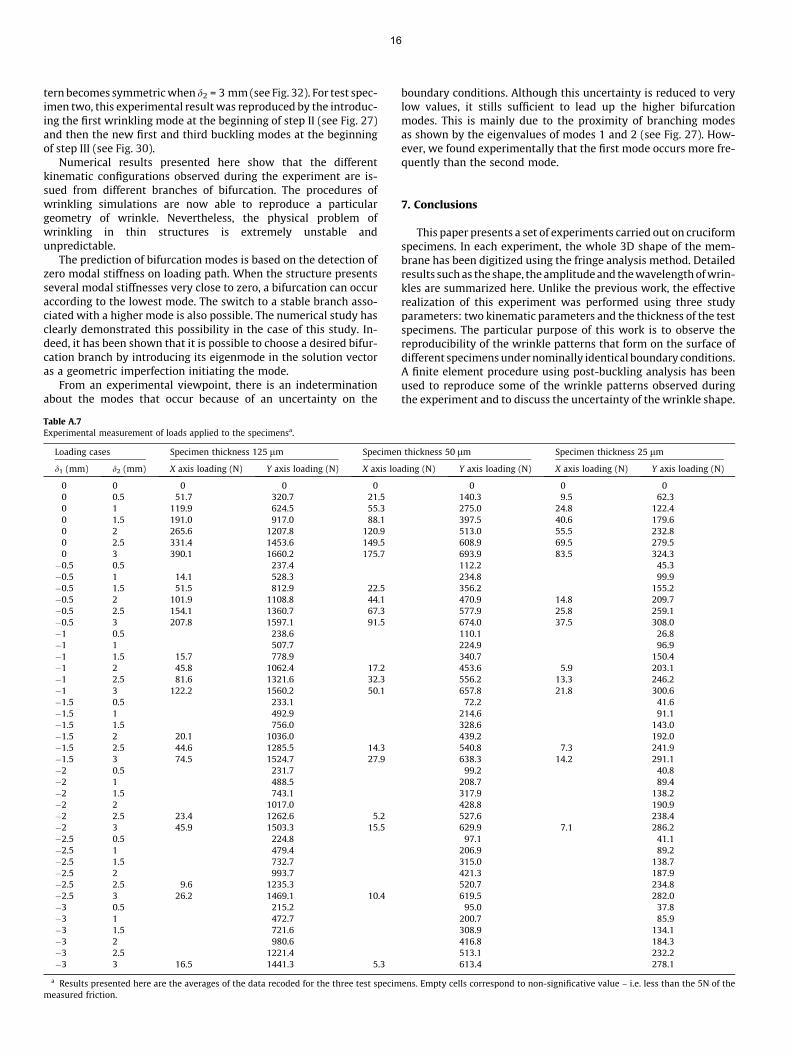
Table A.7Experimental measurement of loads applied to the specimensa.

Loading cases Specimen thickness 125 lm Specimen

d1 (mm) d2 (mm) X axis loading (N) Y axis loading (N) X axis loa

0 0 0 0 00 0.5 51.7 320.7 21.50 1 119.9 624.5 55.30 1.5 191.0 917.0 88.10 2 265.6 1207.8 120.90 2.5 331.4 1453.6 149.50 3 390.1 1660.2 175.7�0.5 0.5 237.4�0.5 1 14.1 528.3�0.5 1.5 51.5 812.9 22.5�0.5 2 101.9 1108.8 44.1�0.5 2.5 154.1 1360.7 67.3�0.5 3 207.8 1597.1 91.5�1 0.5 238.6�1 1 507.7�1 1.5 15.7 778.9�1 2 45.8 1062.4 17.2�1 2.5 81.6 1321.6 32.3�1 3 122.2 1560.2 50.1�1.5 0.5 233.1�1.5 1 492.9�1.5 1.5 756.0�1.5 2 20.1 1036.0�1.5 2.5 44.6 1285.5 14.3�1.5 3 74.5 1524.7 27.9�2 0.5 231.7�2 1 488.5�2 1.5 743.1�2 2 1017.0�2 2.5 23.4 1262.6 5.2�2 3 45.9 1503.3 15.5�2.5 0.5 224.8�2.5 1 479.4�2.5 1.5 732.7�2.5 2 993.7�2.5 2.5 9.6 1235.3�2.5 3 26.2 1469.1 10.4�3 0.5 215.2�3 1 472.7�3 1.5 721.6�3 2 980.6�3 2.5 1221.4�3 3 16.5 1441.3 5.3

a Results presented here are the averages of the data recoded for the three test specimmeasured friction.

boundary conditions. Although this uncertainty is reduced to verylow values, it stills sufficient to lead up the higher bifurcationmodes. This is mainly due to the proximity of branching modesas shown by the eigenvalues of modes 1 and 2 (see Fig. 27). How-ever, we found experimentally that the first mode occurs more fre-quently than the second mode.

7. Conclusions

This paper presents a set of experiments carried out on cruciformspecimens. In each experiment, the whole 3D shape of the mem-brane has been digitized using the fringe analysis method. Detailedresults such as the shape, the amplitude and the wavelength of wrin-kles are summarized here. Unlike the previous work, the effectiverealization of this experiment was performed using three studyparameters: two kinematic parameters and the thickness of the testspecimens. The particular purpose of this work is to observe thereproducibility of the wrinkle patterns that form on the surface ofdifferent specimens under nominally identical boundary conditions.A finite element procedure using post-buckling analysis has beenused to reproduce some of the wrinkle patterns observed duringthe experiment and to discuss the uncertainty of the wrinkle shape.

thickness 50 lm Specimen thickness 25 lm

ding (N) Y axis loading (N) X axis loading (N) Y axis loading (N)

0 0 0140.3 9.5 62.3275.0 24.8 122.4397.5 40.6 179.6513.0 55.5 232.8608.9 69.5 279.5693.9 83.5 324.3112.2 45.3234.8 99.9356.2 155.2470.9 14.8 209.7577.9 25.8 259.1674.0 37.5 308.0110.1 26.8224.9 96.9340.7 150.4453.6 5.9 203.1556.2 13.3 246.2657.8 21.8 300.6

72.2 41.6214.6 91.1328.6 143.0439.2 192.0540.8 7.3 241.9638.3 14.2 291.1

99.2 40.8208.7 89.4317.9 138.2428.8 190.9527.6 238.4629.9 7.1 286.2

97.1 41.1206.9 89.2315.0 138.7421.3 187.9520.7 234.8619.5 282.0

95.0 37.8200.7 85.9308.9 134.1416.8 184.3513.1 232.2613.4 278.1

ens. Empty cells correspond to non-significative value – i.e. less than the 5N of the

17

From the experiment and the simulations, the following conclu-sions can be stated:

� A mechanism of wrinkle division has been observed during theexperiment. The creation of a new wrinkle has been explainedas a local mode change or a local buckling of an existingwrinkle.� Non-unique wrinkle shapes have been observed over repeated

experiments. The comparison with the numerical analysisshowed that the different shapes of wrinkling experimentallyobserved match the numerical predictions issued of differentbranches of bifurcation.

Acknowledgments

Financial support from CNES and EADS Astrium is gratefullyacknowledged. The author thank S. Kervision and C. Lemaire foruseful corrections.

Appendix A

See Table A.7.

References

Balmforth, N.J., Craster, R.V., Slim, A.C., 2008. On the buckling of elastic plates.Quarterly Journal of Mechanics and Applied Mathematics 61 (2), 267–289. URL<http://qjmam.oxfordjournals.org/cgi/content/abstract/61/2/267> .

Blandino, J., Jonhston, J., Miles, J., Soplop, J., 2001. Thin film membrane wrinklingdue to mechanical and thermal loads. In: 42th AIAA/ASME/ASCE/AHS/ASCStructures, Structural Dynamics and Material Conference and Exhibit.

Blandino, J., Jonhston, J., Miles, J., Dharamsi, U., 2002a. The effect of asymmetricmechanical loading on membrane wrinkling. In: 43th AIAA/ASME/ASCE/AHS/ASC Structures, Structural Dynamics and Material Conference and Exhibit.

Blandino, J.R., Johnston, J.D., Dharasi, U.K., 2002b. Corner wrinkling of a squaremembrane due to symmetric mechanical loads. Journal of Spacecraft andRockets 39 (5), 717–724.

Cerda, E., Ravi-Chander, K., Mahadevan, L., 2002. Thin films: winkling of an elasticsheet under tension. Nature 419, 579–580. URL <http://dx.doi.org/10.1038/419579b> .

Crisfield, M., 1997. Non-Linear Finite Element Analysis of Solids and Structures:Advanced Topics. John Wiley & Sons, Inc., New York, NY, USA.

DuPont, 2006. Dupont kapton vn polyimide film technical data sheet. Tech. rep.,DuPont.

Epstein, M., Forcinito, M.A., 2001. Anisotropic membrane wrinkling: theory andanalysis. International Journal of Solids and Structures 38 (30–31), 5253–5272.

Holo3, December 2006. Logiciel FAF FringeAnalysis. Holo3.Jenkins, C., 2001. Gossamer Spacecraft: Membrane and Inflatable Structures

Technology for Space Applications. AIAA.Jenkins, C., Haugen, F., Spicher, W., 1998. Experimental measurement of wrinkling

in membranes undergoing planar deformation. Experimental Mechanics 38,147–152.

Kang, S., Im, S., 1997. Finite element analysis of wrinkling membranes. Journal ofApplied Mechanics 64, 263–269.

Mansfield, E.H., 1968. Tension field theory: a new approach which shows its dualitywith inextensional theory. In: XII Int. Cong. Appl. Mech., pp. 305–320.

Mansfield, E.H., 1970. Load transfer via a wrinkled membrane. In: Proceeding of theRoyal Society.

Mikulas, M.M., 1964. Behavior of a flat stretched membrane wrinkled by therotation of an attached hub. Tech. rep. D-2456, NASA.

Miyamura, T., 2000. Wrinkling on stretched circular membrane under in-planetorsion: bifurcation analyses and experiments. Engineering Structures 22 (11),1407–1425.

Pipkin, A., 1986. The relaxed energy density for isotropic elastic membranes. IMAJournal of Applied Mathematics 36, 8599.

Riks, E., 1979. An incremental approach to the solution of snapping and bucklingproblems. International Journal of Solids and Structures 15 (7), 529–551.

Robinson, D.W., Reid, G., 1993. Interferogram Analysis Digital Fringe PatternMeasurement Techniques. Institute of Physics Publishing.

Stein, M., 1959. Loads and deformation of buckled rectangular plates. Tech. rep. R40.National Aeronautics and Space Administration.

Stein, M., Hedgepeth, J., 1961. Analysis of partly wrinkled membranes. Tech. rep. D-813, NASA.

Surrel, J., Surrel, Y., 1998. La technique de projection de franges pour la saisie desformes d’objets biologiques vivants. Journal of Optics 29 (1), 6–13.

Wagner, H., 1929. Flat sheet metal girders with very thin metal web. Tech. rep. 604,National Advisory Committee for Aeronautics.

Wang, C., Du, X., Tan, H., He, X., 2009. A new computational method for wrinklinganalysis of Gossamer space structures. International Journal of Solids andStructures 46 (6), 1516–1526.

Wong, Y., Pellegrino, S., 2006a. Wrinkled membranes part I: experiments. Journal ofMechanics of Materials and Structures 1, 1–23.

Wong, Y., Pellegrino, S., 2006b. Wrinkled membranes part III: numericalsimulations. Journal of Mechanics of Materials and Structures 1, 61–93.

Yoshizawa, T., 2009. Handbook of Optical Metrology: Principles and Applications.CRC Press.

Zhang, Z., Zhang, D., Peng, X., 2004. Performance analysis of a 3d full-field sensorbased on fringe projection. Optics and Lasers in Engineering 42 (3), 341–353.