experimental study and modelling of...
TRANSCRIPT
Helsinki University of Technology Publications in Materials Science and Engineering Teknillisen korkeakoulun materiaalitekniikan julkaisuja
Espoo 2007 TKK-MT-196
EXPERIMENTAL STUDY AND MODELLING OF VISCOSITY
OF CHROMIUM CONTAINING SLAGS
Doctoral Thesis
Lasse Forsbacka
Helsinki University of Technology Publications in Materials Science and Engineering Teknillisen korkeakoulun materiaalitekniikan julkaisuja
Espoo 2007 TKK-MT-196
EXPERIMENTAL STUDY AND MODELLING OF VISCOSITY
OF CHROMIUM CONTAINING SLAGS
Lasse Forsbacka
Dissertation for the degree of Doctor of Science in Technology to be presented with due permission of the Department of Materials Science and Engineering, Helsinki University of Technology for public examination and debate at Helsinki University of Technology (Espoo, Finland) on the 7th of December, 2007, at 12 o’clock noon.
Helsinki University of Technology
Department of Materials Science and Engineering Laboratory of Metallurgy
Teknillinen korkeakoulu Materiaalitekniikan osasto Metallurgian laboratorio

Available in pdf-format at http://lib.tkk.fi/Diss
Distribution:
Helsinki University of Technology Outokumpu Tornio Works Oy
Laboratory of Metallurgy Lasse Forsbacka
P.O. Box 6200 FI-95400 Tornio, Finland
FI-02015 TKK, Finland
Tel. +358 9 451 2756 +358 16 455 756 +358 40 834 2357
Fax +358 9 451 2798 +358 16 453 295
email: [email protected] [email protected]
© Lasse Forsbacka
ISBN 978-951-22-9032-1
ISBN 978-951-22-9033-8 (electronic)
ISSN 1455-2329 Picaset Oy Helsinki 2007

ABSTRACT An apparatus was constructed to measure the viscosities of molten slags at high temperatures up to 1750 °C. Techniques and methods of viscosity measurement for chromium containing slags were developed using a concentric rotating cylinder method in combination with a high temperature furnace. The viscosities were measured for Al2O3-CaO-MgO-SiO2 slags, and for several slag systems containing chromium oxides, from a quasi-binary system CrOx-SiO2 to quasi-ternary and quaternary systems.
At low oxygen partial pressures such as in typical metallurgical processes, the chromium in the slag appears simultaneously as divalent (CrO) and trivalent (CrO1.5) oxides. It was proven that decreasing the oxygen partial pressure in the system by contacting the slag with metallic chromium increased the amount of divalent CrO, which consequently lowered the melting temperature and viscosity of the slag as well. The measured data were used to develop viscosity models based on the Iida model, the modified Iida model, the modified Urbain model and neural network algorithm methods. The Iida model and the modified Iida model performed well for slags with relatively low chromium content, less than 5 wt. %. In favour of the Iida model, it must be remembered that the chromium content in metallurgical slags is normally quite low. Also, the modified Urbain model accurately predicted the viscosities of slags with higher chromium levels. The neural network computation also proved to be a promising approach for predicting viscosities of metallurgical slags.
Keywords: Slag viscosity, viscosity modelling, FeCr-slag, chromium containing slag

PREFACE This work was mainly conducted in the Laboratory of Metallurgy, Helsinki University of Technology during the years 2001-2004.
I would like to thank everyone who has contributed to this work. Professor Lauri Holappa supported my work from its inception by proposing the research subject, helping with funding, serving as a co-writer on the publications and pushing me to finalize this thesis after I started to work in industry and time became a limited resource. Lauri Holappa also introduced me to helpful colleagues such as Professor Takamichi Iida and Professor Yoshifumi Kita from the Osaka University, who explained the details of the Iida model, which was applied in three of my publications. Professor Peter Hayes enabled me to visit the University of Queensland, Brisbane, Australia, where I spent one month constructing the modified Urbain model, which included chromium oxides and magnesia with the help of Dr. Alex Kondratiev and Dr. Evgeni Jak, who initially developed the modified Urbain model. I would also like to gratefully acknowledge Dr. Masashi Nakamoto, who helped with the figures in publication IV and wrote the manuscript for publication V. The laboratory technicians, especially Mr. Timo Piippo, were extremely helpful in constructing the viscosity measurement apparatus. I extend my sincerest gratitude to all of these individuals for their contributions to this work.
Finally, I would like to thank my parents for encouraging me always, and stressing the importance of efforts and achievement.
Tornio, 20th of September 2007 Lasse Forsbacka
TABLE OF CONTENTS
1 INTRODUCTION .............................................................................................................. 1
2 STRUCTURE OF SLAG.................................................................................................. 2
3 DEFINITION OF VISCOSITY ......................................................................................... 4
4 MEASUREMENT OF VISCOSITY................................................................................. 5
5 VISCOSITY MODELS...................................................................................................... 7 5.1 Urbain model and the modified Urbain model ....................................................... 11 5.2 KTH model ............................................................................................................ 14 5.3 Reddy model ......................................................................................................... 16 5.4 CSIRO model ........................................................................................................ 19 5.5 Iida model and the modified Iida model ................................................................ 20 5.6 Models based on optical basicity (NPL) ................................................................ 22 5.7 Pyrosearch quasi-chemical viscosity model.......................................................... 23 5.8 Nakamoto - Tanaka model .................................................................................... 25 5.9 Modelling viscosity of a heterogeneous liquid....................................................... 27
6 EXPERIMENTAL TECHNIQUES AND METHODS .................................................. 28 6.1 Viscosity measurement arrangement.................................................................... 28 6.1.1 Furnace............................................................................................................. 28 6.1.2 Viscometer........................................................................................................ 29 6.1.3 Spindle and crucible ......................................................................................... 29 6.1.4 Furnace atmosphere......................................................................................... 30 6.1.5 Arrangement ..................................................................................................... 33
7 EXPERIMENTAL PROCEDURES............................................................................... 36 7.1 The measurable CrOx oxide systems.................................................................... 36 7.2 Sample preparation............................................................................................... 40 7.3 Viscosity measurement procedure........................................................................ 41 7.4 Sample analysis .................................................................................................... 43
8 SUMMARY OF THE PUBLICATIONS ........................................................................ 44 8.1 Experimental study of the viscosities of selected CaO-MgO-Al2O3-SiO2 slags
and application of the Iida model .......................................................................... 44 8.2 Viscosity of CaO-CrOx-SiO2 slags in relatively high oxygen partial pressure
atmosphere........................................................................................................... 45 8.3 Viscosity of SiO2-CaO-CrOx slags in contact with metallic chromium and
application of the Iida model ................................................................................. 45 8.4 Experimental study and modelling of viscosity of chromium containing slags ...... 45 8.5 Assessment of viscosity of slags in ferrochromium process ................................. 46
9 RESULTS AND ERROR ANALYSIS........................................................................... 46
10 DISCUSSION .................................................................................................................. 51 10.1 Effect of chromium oxide addition on viscosity...................................................... 51 10.2 The applied viscosity models ................................................................................ 55
11 CONCLUSIONS.............................................................................................................. 59
12 REFERENCES................................................................................................................60
13 APPENDICES 13.1 Article I 13.2 Article II 13.3 Article III 13.4 Article IV 13.5 Article V 13.6 Derivation of the Eyring equation for viscosity
13.6.1 Determination of the Maxwell-Boltzmann equation, i.e. the classical law for the distribution of energy
13.6.2 The theory of absolute reaction rates 13.6.3 Reaction rate theory for viscosity 13.7 Derivation of the Bockris equation for viscosity

List of publications
I Forsbacka L., Holappa L., Iida T., Kita Y., Toda Y., Experimental study of viscosities of selected CaO-MgO-Al2O3-SiO2 slags and application of the Iida model, Scandinavian Journal of Metallurgy, Blackwell Publishing, 2003; 32: 273-280.
II Forsbacka L., Holappa L., Viscosity of CaO-CrOx-SiO2 slags in a relatively high oxygen partial pressure atmosphere, Scandinavian Journal of Metallurgy, 2004; 33: 261-268.
III Forsbacka L., Holappa L., Viscosity of SiO2-CaO-CrOx slags in contact with metallic chromium and application of the Iida model, VII International Conference on Molten Slags Fluxes and Salts, Capetown, SAIMM, Johannesburg, 2004, 129-136.
IV Forsbacka L., Holappa L., Kondratiev A., Jak E., Experimental study and modelling of viscosity of chromium containing slags, Steel Research International, 2007; 78, no.9: 676-684.
V Nakamoto M., Forsbacka L., Holappa L., Assessment of viscosity of slags in ferrochromium process, XI International Conference on Innovations in the Ferro Alloy Industry (INFACON XI) vol.1; 2007:159-164.
The author’s contribution to these articles
The author wrote the manuscripts, except for publication V, which was written by M. Nakamoto. The author provided the experimental viscosity data presented in publications I, II and III. For publications IV and V, the viscosities of the chromium containing slags were measured by the author, and the viscosity data of MgO containing slags were gathered by the literature review performed by the author. The author constructed the viscosity models in publications I, II, III and IV, under the instruction of the co-authors.

INTRODUCTION
1 INTRODUCTION The consumption of stainless steel is growing rapidly, at the highest rate of all metals. During the last decade, the melting and rolling capacity of stainless steel has increased significantly, especially because of huge investments in China. The production and supply of the necessary raw materials, especially nickel, has not increased to meet rising demand, which has resulted in a substantial increase in the price of the most expensive raw material used in austenitic stainless steel. The end-users of stainless steel are not happy about these price increases and are constantly looking for cheaper substitutes, such as plastic, aluminium, galvanized and/or painted carbon steels, and also stainless steel grades with low nickel contents. The profit margin per unit produced decreases with growing production and competition, and all means are necessary to defend profit margin in such a fierce competitive environment. The European producers have been forced to start making nickel free ferritic stainless steels (e.g., 1.4509) and manganese alloyed austenitic steels (e.g., 200-series/1.4432). They are also developing special grades, which combine high corrosion resistance with improved strength, with corresponding weight and cost savings, such as duplex stainless steels. All of these alternatives may substitute for the traditional high nickel containing austenitic steel grades in specific applications at a lower cost. The most important factor in the ability of a particular stainless steel producer to obtain a competitive edge is the production efficiency. New integrated production lines are run with only a few operators, such as Outokumpu Tornio Works cold rolling mill 2 (also called RAP5), which is a fully integrated rolling-annealing-pickling line. All failures in production are identified, and actions are taken to improve processes and product quality.
One of the key issues is to achieve better raw material yield throughout the entire process. Recovery of chromium is of special importance because chromium is the major alloying element in stainless steel. Chromium is alloyed into the stainless steel as ferrochromium, which is produced in a submerged arc-furnace (SAF). SAF is a combination of blast furnace and electric arc furnace, which provides enough energy to reduce the stable chromite pellets and lumpy ore into metallic ferrochromium. The reduction of chromite occurs in two distinct stages. The first occurs between solid chromite, coke and carbon monoxide, and the second occurs in the Al2O3-CaO-MgO-SiO2 based slag. The liquid slag dissolves the already partially reduced solid chromite as the ionic species Cr2+, Cr3+, Fe2+ Fe3+ and O2-, along with some additional impurity elements. Carbon reacts with oxygen anions in the slag and forms carbon monoxide gas (CO). As a consequence, the slag supersaturates with respect to cations. The iron and chromium cations, which comprise the less stable oxides in the slag, are reduced and preferentially precipitated out of the slag, forming metal droplets. The metal droplets coalesce and disperse out of the slag as a heavier phase and collect onto the bottom of the furnace as ferrochromium melt. The chromium yield depends on the thermodynamic reaction equilibrium between the slag and ferrochromium, but also on the reaction kinetics. The thermodynamics of Cr-containing slags were studied by Yanping Xiao in her thesis [1], and chromite reduction kinetics in the solid and liquid states have been studied by Marko Kekkonen [2]. In particular, low viscosity slag speeds up the reactions and helps the metal droplets to segregate out of the slag, which consequently improves the yield of the ferrochromium process, but also the recovery of chromium and other metals in stainless steel melting in an electric-arc-furnace.
There is little previously published data regarding the viscosity of chromium containing slags. Some research was conducted in the late Soviet Union on the viscosities and electrical conductivities of ferrochrome process slags mainly by Zhilo et al. [3,4,5,6,7]. Unfortunately, the compositional analysis in these studies did not separate the different oxidation stages of
1
STRUCTURE OF SLAG
chromium. A comparative analysis with the present study also raises doubt about the viscometer, which was not sensitive enough to detect below 0.2 cPa. The main reasons for the lack of experimental viscosity data are: 1) the high melting temperature of chromium containing slags, which often exceeds the heating range of the experimental furnaces or limits of the available construction materials, and 2) the multiple oxidation stages of chromium (Cr2+, Cr3+, Cr4+, Cr6+), which add a degree of difficulty due to demanding atmospheric control. In reducing conditions, such as in the ferrochromium process, the chromium appears simultaneously as Cr2+ (CrO) and Cr3+ (CrO1.5). The distribution of the total chromium content (CrOx) into CrO and CrO1.5 is dependent on the oxygen partial pressure, the temperature, and the total amount of chromium and other oxide species in the slag. The low PO2 increases the portion of CrO and lowers the liquidus temperature of the slag. The viscosity measurements are very expensive to perform because of the high temperature refractory materials which often can only be used for a limited time. These measurements are also very time-consuming due to the long heating and cooling times of furnaces, along with sample preparation and analysis. Furthermore, the experimental runs often fail, and the results are subject to fairly large errors [8].
Mathematical viscosity models may be used to interpolate the viscosity values at compositions where the measured data does not exist, or extrapolate the viscosity data to the composition ranges where the measurement could not be made in practice due to the high melting temperatures. A successful viscosity model can also decrease the errors of independent measurements, and may provide more reliable data than a separate measurement alone. The viscosity model may be incorporated with thermodynamic and kinetic computer aided models, and used to model and optimise real production processes.
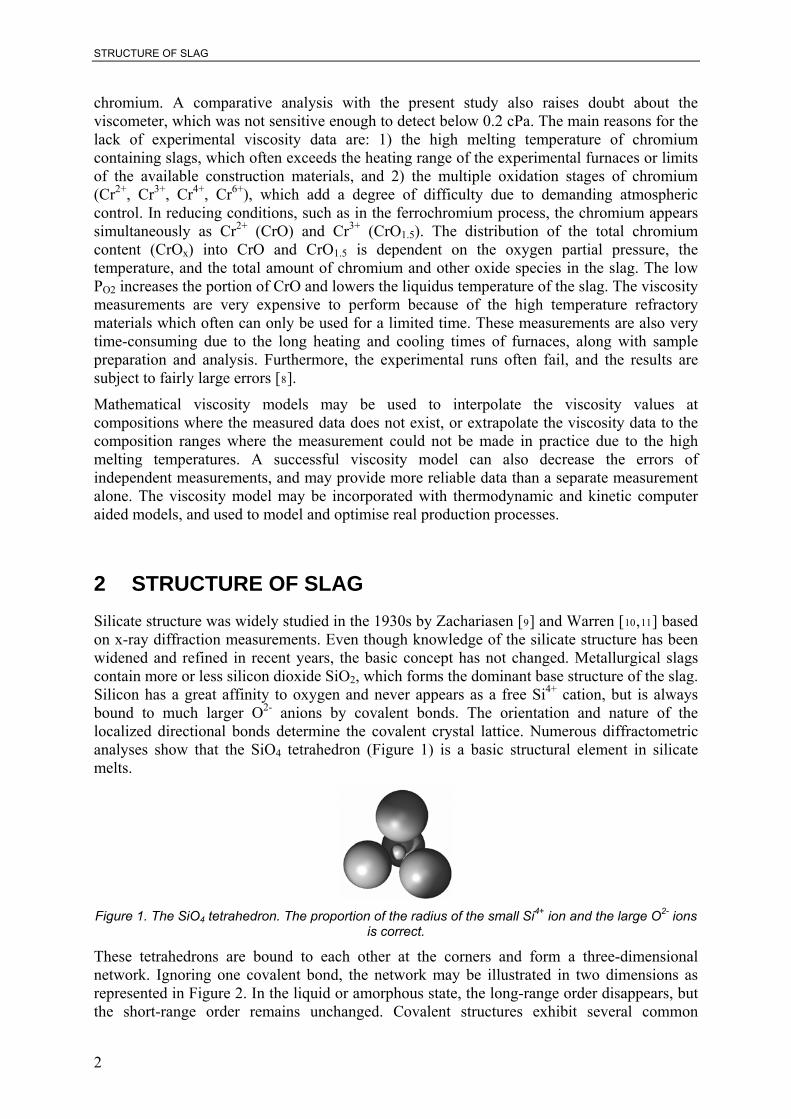
2 STRUCTURE OF SLAG Silicate structure was widely studied in the 1930s by Zachariasen [9] and Warren [10,11] based on x-ray diffraction measurements. Even though knowledge of the silicate structure has been widened and refined in recent years, the basic concept has not changed. Metallurgical slags contain more or less silicon dioxide SiO2, which forms the dominant base structure of the slag. Silicon has a great affinity to oxygen and never appears as a free Si4+ cation, but is always bound to much larger O2- anions by covalent bonds. The orientation and nature of the localized directional bonds determine the covalent crystal lattice. Numerous diffractometric analyses show that the SiO4 tetrahedron (Figure 1) is a basic structural element in silicate melts.
Figure 1. The SiO4 tetrahedron. The proportion of the radius of the small Si4+ ion and the large O2- ions
is correct.
These tetrahedrons are bound to each other at the corners and form a three-dimensional network. Ignoring one covalent bond, the network may be illustrated in two dimensions as represented in Figure 2. In the liquid or amorphous state, the long-range order disappears, but the short-range order remains unchanged. Covalent structures exhibit several common
2

STRUCTURE OF SLAGS
macroscopic features; they are extremely hard and difficult to deform in the solid state, and the bonds remain strong in the liquid state. Therefore, the viscosity of molten silicate is very high, as illustrated by common window glass.
Figure 2. Schematic representation of the SiO2 crystal lattice in the solid state (left) and the structure in the liquid state. Figures adapted from Richardson [12].
When a basic oxidei [13] MO or M2O is added to a slag based on SiO2, where element M is K, Na, Li, Ca, Mg, Fe, Mn, Pb, Zn, Ni or Cu, the basic oxide strives to dissociate into metallic cations and oxygen anions. These extra O2- anions bond with silicon in the SiO2 structure and break up the network, as shown in Figure 3.
Figure 3. The de-polymerisation reaction of silica by basic oxides [12].
With small additions of basic oxide, the oxygen remains bound to the silicate molecule by one covalent bond (O-), but is negatively charged. If more and more basic oxide is added, free oxygen (O2-) ions will eventually appear, as represented in Figure 4.
Figure 4. The de-polymerisation reaction of silica by basic oxides until free oxygen (O2-) appears in the
structure.
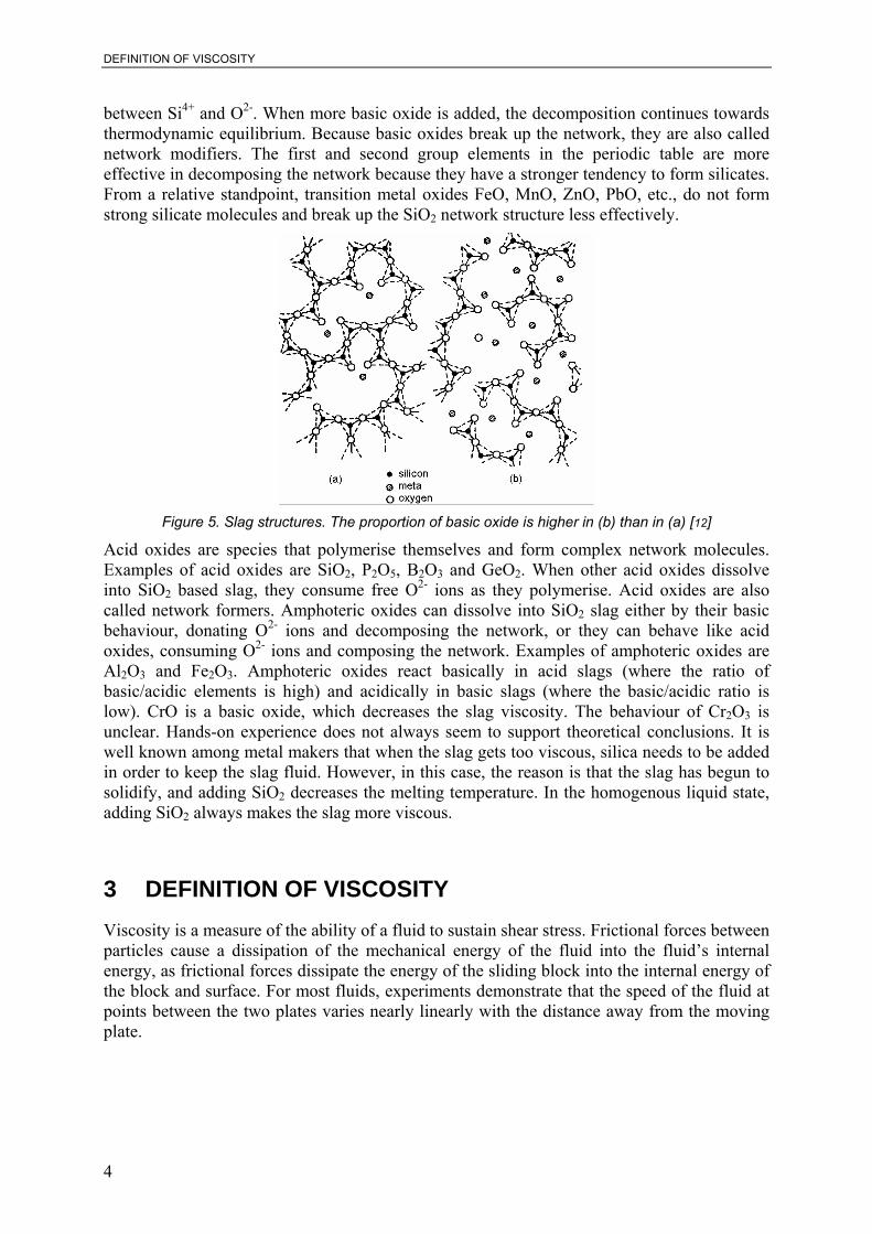
As the network decomposes, the viscosity decreases (Figure 5) because the bond between M2+ and O2- is ionic in nature, is not well oriented and is clearly weaker than the covalent bond
i The concept of basicity is defined analogously with water solutions; as (acid = base + H+) in water solutions, (base = acid + O2-) in silicate solutions.
3
DEFINITION OF VISCOSITY
between Si4+ and O2-. When more basic oxide is added, the decomposition continues towards thermodynamic equilibrium. Because basic oxides break up the network, they are also called network modifiers. The first and second group elements in the periodic table are more effective in decomposing the network because they have a stronger tendency to form silicates. From a relative standpoint, transition metal oxides FeO, MnO, ZnO, PbO, etc., do not form strong silicate molecules and break up the SiO2 network structure less effectively.
Figure 5. Slag structures. The proportion of basic oxide is higher in (b) than in (a) [12]
Acid oxides are species that polymerise themselves and form complex network molecules. Examples of acid oxides are SiO2, P2O5, B2O3 and GeO2. When other acid oxides dissolve into SiO2 based slag, they consume free O2- ions as they polymerise. Acid oxides are also called network formers. Amphoteric oxides can dissolve into SiO2 slag either by their basic behaviour, donating O2- ions and decomposing the network, or they can behave like acid oxides, consuming O2- ions and composing the network. Examples of amphoteric oxides are Al2O3 and Fe2O3. Amphoteric oxides react basically in acid slags (where the ratio of basic/acidic elements is high) and acidically in basic slags (where the basic/acidic ratio is low). CrO is a basic oxide, which decreases the slag viscosity. The behaviour of Cr2O3 is unclear. Hands-on experience does not always seem to support theoretical conclusions. It is well known among metal makers that when the slag gets too viscous, silica needs to be added in order to keep the slag fluid. However, in this case, the reason is that the slag has begun to solidify, and adding SiO2 decreases the melting temperature. In the homogenous liquid state, adding SiO2 always makes the slag more viscous.
3 DEFINITION OF VISCOSITY Viscosity is a measure of the ability of a fluid to sustain shear stress. Frictional forces between particles cause a dissipation of the mechanical energy of the fluid into the fluid’s internal energy, as frictional forces dissipate the energy of the sliding block into the internal energy of the block and surface. For most fluids, experiments demonstrate that the speed of the fluid at points between the two plates varies nearly linearly with the distance away from the moving plate.
4

MEASUREMENT OF VISCOSITY
Figure 6. Model of viscous flow. When the upper plate is pulled slowly at a constant speed, the viscous
fluid between the plates flows in lamina, and the speed is proportional to the distance from the stationary plate at the bottom.
Fluids for which the horizontal force component required to move the plate is proportional to the speed of the plate are called Newtonian fluids. The magnitude of the force F on the moving plate depends not only on the speed v of the moving plate, but is also proportional to the area of plate A and inversely proportional to the distance l between the moving and stationary plates [14].
lAvF η
= (1)
A constant of proportionality η (sometimes μ) is called the dynamic viscosity. The SI unit for viscosity is Pas (Nsm-2). A common non-SI unit for viscosity is P (poise), equal to 0.1 Pas. In many scenarios, it is practical to use a quantity called the kinematic viscosity ν, which is viscosity divided by density (ν = μ / ρ). The SI unit for kinematic viscosity is m2s-1, and a common non-SI unit is St (stoke), equal to 0.0001 m2s-1. All gases and most simple liquids, including molten metals and most metallurgical slags, obey Newtonian behaviour in the homogenous liquid state [15]. Those fluids that do not closely obey the linear proportionality of the speed and force to be fitted in equation 1 are called non-Newtonian fluids. Examples of non-Newtonian fluids are certain plastics and suspensions such as blood and water-clay mixtures, and liquids that are not homogenous such as partly solidified slag in the mushy zone.
4 MEASUREMENT OF VISCOSITY The concentric cylinder method using molybdenum or platinum components provides the most accurate results for measurements of slag viscosities at high temperatures in a ‘round robin’ test coordinated by BCR (Bureau Communautaire de Référence) [8,16].
Figure 7. Concentric cylinder method [17].
5

MEASUREMENT OF VISCOSITY
In the concentric cylinder method, the slag is contained in an annular gap between two concentric cylinders and either the spindle (the inner cylinder) or the crucible (the outer cylinder) is rotated at a constant speed. The viscosity of the fluid transmits a torque, and the viscosity is calculated from the measured torsional resistance. If the laminar Couett flow occurs between two coaxial cylinders, absolute viscosity can be calculated according to equation [18]:
ηπ
= −⎛
⎝⎜
⎞
⎠⎟
Mnh r ri o8
1 12 2 2
(2)
where M = torque, n = revolutions, h = height of the cylinder, ri = radius of the inner cylinder and ro = radius of the outer cylinder measured surface. The equation is valid for infinitely long cylinders and does not take into account the error resulting from the boundary effect. G.F.C. Searle showed that complete elimination of the boundary effect can be achieved by differential immersion of cylinders in the liquid and measurement of the difference in transferred torque at constant revolution speed [18]. The viscosity is obtained as:
( )η
π=
−−
−⎛
⎝⎜
⎞
⎠⎟
M Mn h h r ri o
1 22
1 22 28
1 1 (3)
In practice, it is more convenient to calibrate the equipment with a liquid of known viscosity. This method eliminates errors that would be difficult to express in the form of an equation and may vary between test runs, such as boundary effects, displacement of concentric cylinders and spindle sway. In the present study, re-calibration was necessary for new spindles even when they were made with the same dimensions. In principle, the calibration is done by defining the system-dependent constant, which relates the applied force to viscosity. Instead of the force, electric voltage, torque or any other measure of applied force can be used depending on the display configuration:
Saa
UaFa
4
3
2
1
====
ητη
ηη
(4)
where (a) is a system dependent constant, (F) is force, (U) is voltage, (τ) is torque and (S) is any measure of force which causes the defined deflection of the measurement scale. As the applied force (equation 1) is proportional to the speed, or in this case, the spindle rotational speed, the equation for Newtonian fluids may be represented as:
nSG ×=η (5)
where G = cell constant, S = scale deflection and n = speed of rotation. The easiest method to determine the system constant (or cell constant) is to use three or more standard viscosity fluids and measure the applied forces. When viscosity is plotted against the applied force, a straight line should be observed where the slope is the system-dependent constant. Different speeds should give the same value for the constant (for Newtonian fluids), but if there is a deviation, the measurement system may be unstable, e.g., the spindle may sway, either because it is not balanced or because the spindle shaft is not straight. The concentric cylinder method has become the most popular method of viscosity measurement, especially for scientific purposes. There are also other methods such as oscillation of the plate/cylinder [19], falling body and capillary/run-out methods, which have been described in depth in the Slag Atlas [18]. The works of Wilhelm Eitel, “The physical chemistry of the silicates, 1954,” and
6
VISCOSITY MODELS
“Silicate science, 1965,” shed significant light on the historical development of viscosity measurement devices for molten slag [20,21]. For practical purposes, quick and easy methods have been developed to determine the approximate slag viscosities. The Herty viscometer is made of two steel blocks, which are attached to each other. There are vertical and horizontal grooves in the middle interface [18], and these grooves meet such that the slag poured onto the vertical groove runs into the horizontal groove. The distance travelled by the slag before freezing is measured, and an approximation of viscosity is obtained. In the inclined plane method, the melted sample of slag is poured onto an inclined plane. The viscosity is then derived by supposing that it is proportional to the length of the cooled ribbon slag formed on
the plane. This method is used frequently in industry to provide quick and approximate values for comparative purposes [22].
5 VISCOSITY MODELS At the end of the 18th century, Arrhenius found that many temperature dependent processes and properties, such as viscosity, are logarithmically correlated with temperature [23]:
⎟⎠⎞
⎜⎝⎛ Δ
=RT
GAexpμ (6)
where A is a proportionality constant, ΔG is the activation energy for viscous flow, T represents temperature and R is the universal gas constant. Later, the viscosity equation was derived from basic fundamental principles of physics. The most famous solutions were conducted by Eyring based on absolute reaction rate theory (equation 7, Appendix 1) [24], Bockris and Reddy based on Hole theory (equation 8, Appendix 2) [25], and Weymann based on Hole theory (equation 9) [26]:
η ρ= ⋅ ⎛
⎝⎜⎞⎠⎟
= ⋅ ⎛⎝⎜
⎞⎠⎟
hNV
GRT
hNM
GRTm
exp * exp *Δ Δ (7)
where h = Planck’s constant, N = Avogadro’s number, Vm = molar volume, ΔG* = Gibbs energy of activation of viscous flow, R = the universal gas constant, T = absolute temperature, ρ = density and M = molecular weight.
( )η π= ⟨ ⟩⎛⎝⎜
⎞⎠⎟2
32
12n r mkT eh h
ERT (8)
where nh = number of holes per unit volume, ⟨rh⟩ = the average radius of the holes, m = mass of the ionic unit, k = Boltzmann constant, T = absolute temperature, E = the energy of the ionic unit for viscous flow and R = the universal gas constant.
( )⎟⎠⎞
⎜⎝⎛⋅⋅⎟⎟
⎠
⎞⎜⎜⎝
⎛=
kTE
Pv
mkTERT W
VW
exp2
32
21
21
η (9)
where m and v are the mass and volume of the structural unit, EW the energy well, k and T Boltzmann constant and absolute temperature, and PV is the “hole” probability connected with the structural model of liquid. The above solutions may be expressed in a form sometimes referred to as the general form of the Arrhenius equation, which is distinct from the classical Arrhenius equation:
)/exp( TBAT n=η (10)
7
VISCOSITY MODELS
where n is either 0, ½, or 1 for the Eyring, Bockris & Reddy or Weymann equations, respectively. It may be perceived that the Eyring equation is consistent with the classical Arrhenius equation. These theoretical equations have mainly been applied to liquid metals, which have a simple mono-atomic nature. For more complicated liquids like silicate melts, these equations have not been able to provide satisfactory results. However, the concept of activation energy and the logarithmic relationship between viscosity and temperature offer a very good framework for the further development of viscosity models of complicated silicate melts. It is also common that the handbooks for physico-chemical properties represent the viscosity data as formulas logη=A+B/T or logη=A+B/T+C/T2, instead of providing a separate table of viscosity values at each given temperature. The problem is how to incorporate the influence of composition on viscosity into the viscosity equation. In other words, how can the composition dependent parameters A and B of equation 6 be determined? The first attempt to control slag quality using the theory of silicate melts was to calculate the silicate degree of the slag:
oxidesacidinoxygenofweightoxidesbasicinoxygenofweightdegreeSilicate = (11)
Roberts showed (1959) that the silicate degree does not provide a useful indication of slag quality as far as viscosity is concerned, and suggested that another parameter be used, which he termed the viscosity index [27]:
)%80.0(%)%67.0(% 322
CaOwtFeOwtOAlwtSiOwtindexViscosity
++
= (12)
The factors for SiO2 and FeO were obtained by supposing that FeO and SiO2 have efficiencies equal to unity as fluidity and viscosity increasing oxides, respectively. The factor for lime was calculated as the ratio of the ion-oxygen attractioni of Ca2+ and Fe2+, and for alumina as the ratio of ion-oxygen attraction of Al3+ and Si4+. Using Roberts´ results, Dannat proposed his own parameter, the viscosity ratio, which is used in viscosity quality checking [28]:
at%OAl)at%(SiratioViscosity +
= (13)
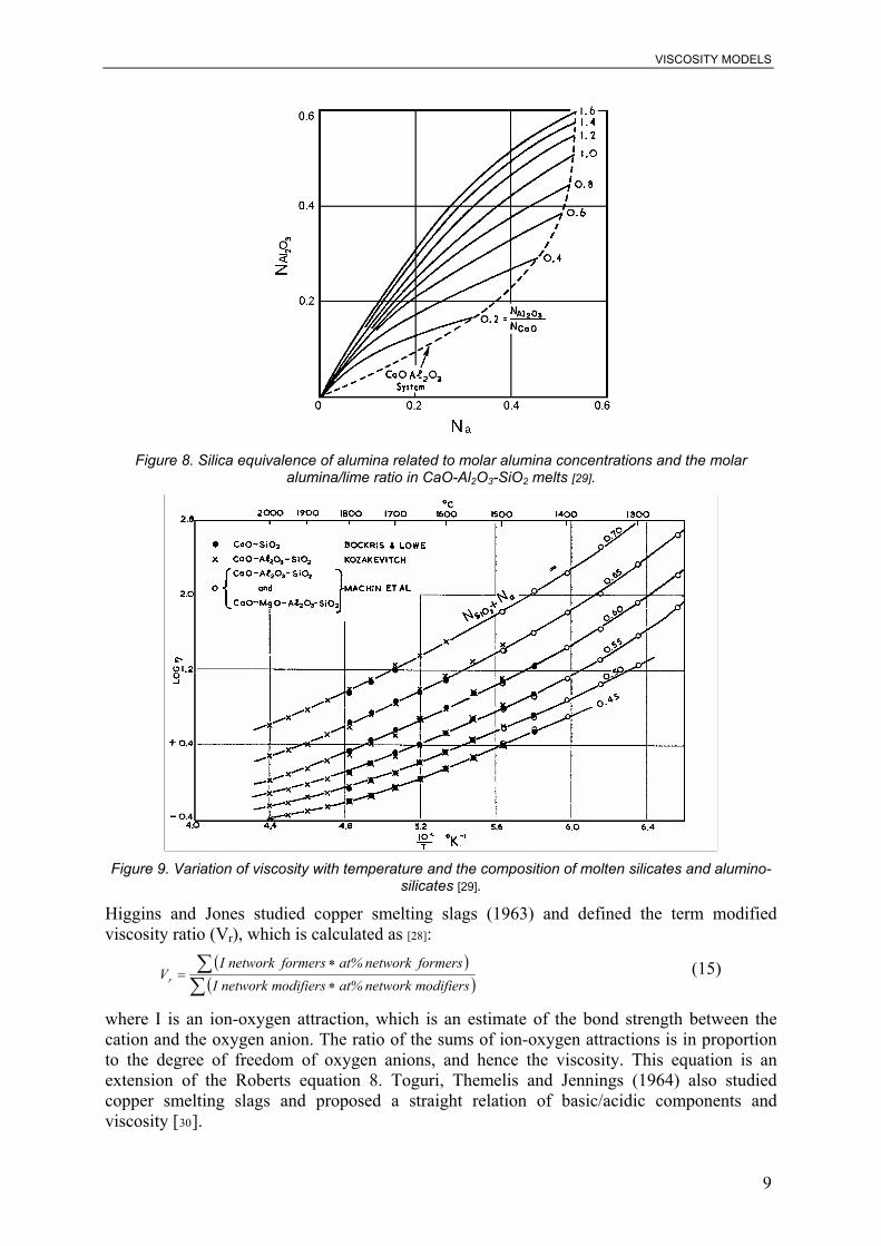
This equation gave a good relationship with Roberts´ results, where silica and alumina were the main constituents of high ion-oxygen attraction. However, for other slags, the relationship is worse. Turkdogan and Bills studied the viscosity of CaO-MgO-Al2O3-SiO2 melts (1960) [29], and introduced a parameter called a silica equivalent. For a given temperature and viscosity, the silica-equivalence of aluminium (Na) is given by the difference between the silica concentrations of the binary (CaO-SiO2) and ternary (CaO -Al2O3-SiO2) melts, i.e..
(ternary)N(binary)NNN2232 SiOSiOaOAl −== (14)
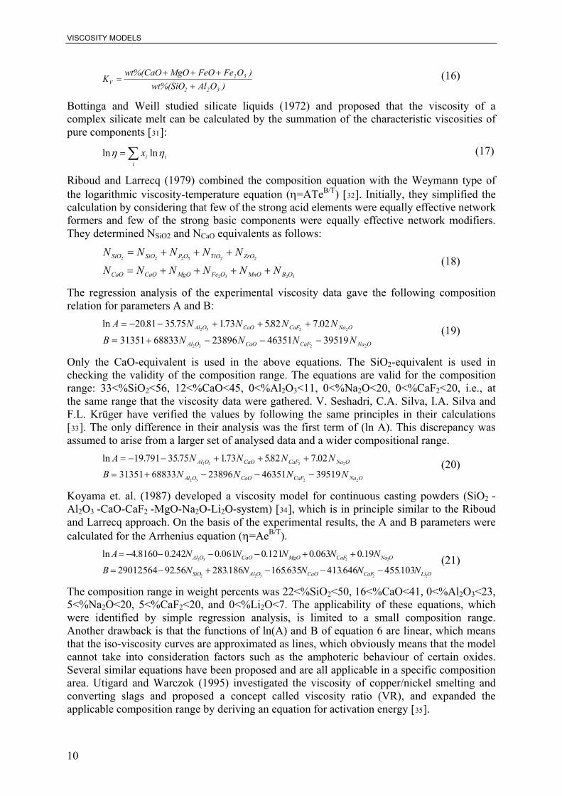
On the basis of earlier studies, Turkdogan and Bills concluded that CaO and MgO are interchangeable in terms of their effects on viscosity. The effect of acid oxide Al2O3 is equal to Na units of SiO2, which is plotted in Figure 8. Any compositional variation of the CaO-MgO-Al2O3-SiO2 solution and the corresponding viscosity at a certain temperature can then be found on the one curve on a graph, where the axis of the abscissa is (Na+NSiO2), and the axis of the ordinate is the viscosity (Figure 9).
i The ion-oxygen attraction = the ionic field strength = Z/a2, where Z = ionisation degree of the cation and a = rc + rO = radius of the cation + radius of the oxygen anion. Coulomb force ∝ Z/a2. The stronger the bond between the cation and oxygen anion, the more acidic the component is.
8
VISCOSITY MODELS
Figure 8. Silica equivalence of alumina related to molar alumina concentrations and the molar
alumina/lime ratio in CaO-Al2O3-SiO2 melts [29].
Figure 9. Variation of viscosity with temperature and the composition of molten silicates and alumino-
silicates [29].
Higgins and Jones studied copper smelting slags (1963) and defined the term modified viscosity ratio (Vr), which is calculated as [28]:
( )( )∑
∑∗
∗=
modifiersnetworkat%modifiersnetworkIformersnetworkat%formersnetworkI
Vr (15)
where I is an ion-oxygen attraction, which is an estimate of the bond strength between the cation and the oxygen anion. The ratio of the sums of ion-oxygen attractions is in proportion to the degree of freedom of oxygen anions, and hence the viscosity. This equation is an extension of the Roberts equation 8. Toguri, Themelis and Jennings (1964) also studied copper smelting slags and proposed a straight relation of basic/acidic components and viscosity [30].
9
VISCOSITY MODELS
)OAlwt%(SiO)OFeFeOMgOwt%(CaO
K322
32V +
+++= (16)
Bottinga and Weill studied silicate liquids (1972) and proposed that the viscosity of a complex silicate melt can be calculated by the summation of the characteristic viscosities of pure components [31]:
∑=i
iix ηη lnln (17)
Riboud and Larrecq (1979) combined the composition equation with the Weymann type of the logarithmic viscosity-temperature equation (η=ATeB/T) [32]. Initially, they simplified the calculation by considering that few of the strong acid elements were equally effective network formers and few of the strong basic components were equally effective network modifiers. They determined NSiO2 and NCaO equivalents as follows:
3232
225222
OBMnOOFeMgOCaOCaO
ZrOTiOOPSiOSiO
NNNNNN
NNNNN
++++=
+++= (18)
The regression analysis of the experimental viscosity data gave the following composition relation for parameters A and B:
ln . . . . .A N N N N
B N N NAl O CaO CaF Na O
Al O CaO CaF Na O
= − − +
N
+ +
= + − − −
2081 3575 173 582 7 02
31351 68833 23896 46351 395192 3 2 2
2 3 2 2
(19)
Only the CaO-equivalent is used in the above equations. The SiO2-equivalent is used in checking the validity of the composition range. The equations are valid for the composition range: 33<%SiO2<56, 12<%CaO<45, 0<%Al2O3<11, 0<%Na2O<20, 0<%CaF2<20, i.e., at the same range that the viscosity data were gathered. V. Seshadri, C.A. Silva, I.A. Silva and F.L. Krüger have verified the values by following the same principles in their calculations [33]. The only difference in their analysis was the first term of (ln A). This discrepancy was assumed to arise from a larger set of analysed data and a wider compositional range.
ln . . . . .A N N N N
B N N NAl O CaO CaF Na O
Al O CaO CaF Na O
= − − +
N
+ +
= + − − −
19 791 3575 173 582 7 02
31351 68833 23896 46351 395192 3 2 2
2 3 2 2
(20)
Koyama et. al. (1987) developed a viscosity model for continuous casting powders (SiO2 -Al2O3 -CaO-CaF2 -MgO-Na2O-Li2O-system) [34], which is in principle similar to the Riboud and Larrecq approach. On the basis of the experimental results, the A and B parameters were calculated for the Arrhenius equation (η=AeB/T).
OLiCaFCaOOAlSiO
ONaCaFMgOCaOOAl
NNNNNB
NNNNNA
22322
2232
103.455646.413635.165186.28356.92564.29012
19.0063.0121.0061.0242.08160.4ln
−−−+−=
++−−−−= (21)
The composition range in weight percents was 22<%SiO2<50, 16<%CaO<41, 0<%Al2O3<23, 5<%Na2O<20, 5<%CaF2<20, and 0<%Li2O<7. The applicability of these equations, which were identified by simple regression analysis, is limited to a small composition range. Another drawback is that the functions of ln(A) and B of equation 6 are linear, which means that the iso-viscosity curves are approximated as lines, which obviously means that the model cannot take into consideration factors such as the amphoteric behaviour of certain oxides. Several similar equations have been proposed and are all applicable in a specific composition area. Utigard and Warczok (1995) investigated the viscosity of copper/nickel smelting and converting slags and proposed a concept called viscosity ratio (VR), and expanded the applicable composition range by deriving an equation for activation energy [35].
10

VISCOSITY MODELS
222232
322322
6.17.0)(3.27.08.0)(5.02.18.12.15.1
,
CaFOCuOKONaCaOMgOPbOOFeFeOBOAlZrOOCrSiOA
whereBAVR
++++++++=+++=
= (22)
Regression analysis of the viscosity data at 1300 ºC gave the following equation:
968.0,59.282.2)(log 25.0 =⋅+−= RVRPasη (23)
This relationship was derived from the graph which depicted viscosity versus the inverse of the absolute temperature, which showed that the slope of the activation energy increases with increasing viscosity. The activation energies of several slags were plotted against the logarithm of viscosity at 1300 ºC, which clearly showed a correlation. The following equation for this trend was found by the least square method.
88.0),(log5.894.182)/( 2 =⋅+= RPasmolkJEa η (24)
By combining equations 23 and 24, viscosity can be calculated as a function of temperature and composition:
)(1208036601.549.0)(log
5.05.0
KTVRVRPas +−
+−−=η (25)
More sophisticated approaches have been developed to represent the viscosity of any silicate melt composition, including the effect of amphoteric oxides. The structure related parameters A and B of the Arrhenius equation are expressed with apparently structure related equations, which often contain polynomial series. Polynomial series can be set to follow any continuous phenomenon, such as viscosity as a function of temperature, by adjusting the polynomial constants. Each structural component or oxide has a set of constants or so called ‘viscosity parameters’, which can be deduced from experimental data. Polynomial series, i.e., viscosity parameters, can be summed to represent the viscosity of multi-component slags.
5.1 Urbain model and the modified Urbain model G. Urbain (1981) conducted a viscosity expression starting from the statistical viscosity model proposed by H.D. Weymann (equation 9) [36, 37]. The two parameters A and B in equation 10 were related to the composition, which was first simplified by dividing components into glass forming, modifying and amphoteric cations, and calculating the equivalent composition of each element. H.D. Weymann constructed viscosity equation 9 on the basis of the hole theory of liquids, according the ‘hole’ probability Pv, which is proportional to the concentration Nv of ‘holes’ given at T by the equilibrium:
⎟⎠⎞
⎜⎝⎛ Δ−
⋅⎟⎠⎞
⎜⎝⎛ Δ
=RT
HRSN V
V expexp (26)
where ΔHV and ΔSV are the partial molar enthalpy and entropy associated with ‘hole’ formation. Parameters A and B expressed in equation 10 in molar quantities are:
( ) ⎟⎠⎞
⎜⎝⎛ Δ−
⎟⎠⎞
⎜⎝⎛
⎟⎟⎠
⎞⎜⎜⎝
⎛=
kS
vmk
EkA V
w
exp1232
212
1
(27)
RHE Vw Δ+
=B . (28)
The “hole” equilibrium is governed by the free energy:
11

VISCOSITY MODELS
VVV STHTG Δ−Δ=Δ )( (29)
At the ‘critical’ temperature T=TC, the free energy becomes zero (ΔGV=0) and the equation can be written as:
C
VV T
HS Δ=Δ (30)
which is also valid for the partial molar quantities. To simplify the notation:
32
21
012
⎟⎠⎞
⎜⎝⎛
⎟⎟⎠
⎞⎜⎜⎝
⎛=
vEmkAw
(31)
Substituting equation 31 into equation 27 after taking the logarithm:
kSAA vΔ
−= 0ln (32)
and substituting equation 30 into 32, we obtain:
c
v
kTHAA Δ
−= 0lnln (33)
Again, substituting equation 28 into 33 gives:
CC
w
TB
kTEAA −+= 0lnln (34)
where A0, E and TC are constants for a given liquid. A simple formulation is:
nBmA +⋅=− ln (35)
The parameters m and n may be deduced from the experimental parameters A and B. Each liquid has a specific m and n value, but Urbain found that for similar liquids, the m and n values were close to each other. For hydrogen bonded liquids, such as methanol, ethanol, water, mineral oils, glycerol and glucose, the mean value of m was 2.427 and n was 11.457. For network liquids (B2O3, GeO2, SiO2), m=0.207 and n=10.288. From a group of 54 ionic liquids (oxides, silicates and alumino-silicates), Urbain calculated mean values for m and n to be 0.293 and 11.571, respectively. If the slag is extremely acidic and the fraction of network formers is 0.85 to 0.90 mole fraction of tetrahedral TO2 (see the next paragraph), the liquid behaves more like a pure network liquid, and the m and n parameters must be changed accordingly. A linear equation allows for the calculation of the viscosity at temperature T if the enthalpy parameter B is known. The model of viscosity estimation is now limited to an interpolation of B with the composition of the slag. Urbain classified all cations into the three categories of glass formers, modifiers and amphoteric cations:
- Glass formers are Si4+, Ge4+, P5+, etc., forming poly-anions SiO44-, Si2O7
6-, PO43-, etc.
- Modifiers are Na+, K+, Mg2+, Ca2+, Fe2+, Cr3+, Ti4+, etc. - Amphoteric cations are Al3+ and Fe3+.
Chemical analysis gives the weight percentage of each component. Mole fractions are calculated and normalized to unity and the equivalent mole fraction is obtained for a hypothetical ternary TO2-A2O3-MO, where T is a glass former, A is an amphoteric cation and M is a modifier cation associated with one oxygen. For example, in a slag with only silicon as a network former, it is clear that T=Si and the mole fractions are the same if there are no
12
VISCOSITY MODELS
changes in the other mole fractions. When silicates and phosphates are present in the slag, T=Si+P:
- analysis gives wt.%(P2O5) - mole fraction is calculated N(P2O5) - charge equivalence T=4/5P, (TO2 refers to structural element TO4
4- ⇒ T4+ equals 4/5P5+) - mole equivalence N(TO2)=8/5N(P2O5) - For this slag N(TO2)=N(SiO2) + 8/5N(P2O5)
For modifier cations M2+ or M+ associated with one oxygen MO or M2O, the mole fractions are equivalent. The mole fraction of trivalent cations N(M2O3) are converted to the equivalent for one oxygen, 3N(M2O3). Tetra-, pentavalent, and higher valency cations are converted according to the relationship N(equi.MO)=yN(MXOY). Changes in the number of moles alter all mole fractions, and normalization to unity is required for further calculations. To enable the estimation of viscosity of a ternary melt, it is necessary to define two compositional parameters, the network former mole fraction X=N(TO2) and α=MO/(MO+ A2O3). B can then be represented by the polynomial equation:
B=B0+B1X+B2X2+B3X3, BI=a(i)+b(i) α+c(i) α2, with i = 0,1,2,3 (36)
It is possible to calculate B for two ternaries: B(Mg) for SiO2-Al2O3-MgO and B(Ca) for SiO2-Al2O3-CaO, and to obtain the mean B for a quaternary melt by considering the B(Mg) and B(Ca) using the mole fractions of N(MgO) and N(CaO). When parameter B is calculated, the viscosity at temperature T(K) can be calculated. According to Urbain, slags (ionic liquids) have very distinctive values of m and n. Kondratiev and Jak challenged this generalization, because it did not provide an accurate description of A and B over the entire compositional range of the studied slag systems [38]. Therefore, they modified the Urbain formalism so that the m value would be a composition dependent variable:
∑= ii Xmm (37)
where mi is a value of pure oxide (Al2O3, CaO, ‘FeO’, SiO2, etc.), and Xi is the mole fraction of the corresponding oxide. Often, experimental viscosity data do not exist for pure oxides because of their high melting temperatures, but it is possible to extrapolate the activation energies (B-parameters) of pure oxides from the binary data (e.g.CaO-SiO2). The n parameter was still considered to be a constant, but a new value was proposed to be 9.322, which was more coherent with the new m values. As a result, Kondratiev and Jak constructed a viscosity model, which was able to predict the viscosities of the Al2O3-CaO-‘FeO’-SiO2 system with good accuracy. As a part of this thesis, the model was expanded to include MgO, CrO and Cr2O3 in order to expand its use to metallurgical processes, where chromium and magnesium are slag constituents. Viscosity η in the modified Urbain model is expressed through the Urbain equation:
⎟⎟⎠
⎞⎜⎜⎝
⎛=
TBA
310expη (38)
where T is the absolute temperature [K], and the pre-exponential term A is linked to the parameter B through the compensation law (m and n are the adjustable parameters):
nmBA +=− ln . (39)
If CrO and Cr2O3 are treated as two different modifiers, expressions for m and B for the Al2O3-CaO-CrO-Cr2O3-‘FeO’-MgO-SiO2 system can be written as follows:
SSMMFFCrCrCrCrCCAA XmXmXmXmXmXmXmm ++++++= '''''''''' (40)
13
VISCOSITY MODELS
iS
j
i j
MFCrCrC
MjMi
MFCrCrC
FjFi
MFCrCrC
CrjCri
MFCrCrC
CrjCri
MFCrCrC
CjCi
i
iSi X
XXXXXXb
XXXXXXb
XXXXXXb
XXXXXXb
XXXXXXb
XbB α∑∑∑= ==
⎟⎟⎟⎟⎟⎟⎟⎟
⎠
⎞
⎜⎜⎜⎜⎜⎜⎜⎜
⎝
⎛
+++++
+++++
+++++
+
+++++
+++++
+=3
0
2
1
'''''
,
'''''
,
'''''
''','''
'''''
'',''
'''''
,
3
0
0
(41)
MFCrCrCA
MFCrCrC
XXXXXXXXXXX+++++
++++=
'''''
'''''α (42)
where XA, XC, XCr’’, XCr’’’, XF, XM, XS are the molar fractions of Al2O3, CaO, CrO, Cr2O3, FeO, MgO and SiO2, respectively; n is a constant; mY, , and (i = 0, 1, 2, 3; j = 1, 2) are the adjustable model coefficients (Y = A, C, Cr’’, Cr’’’, F, M, S). For model consistency, it is necessary that
0ib jY
ib ,
03
0
2
1
,3
0
2
1
,3
0
2
1
,'''3
0
2
1
,''3
0
2
1
, ===== ∑∑∑∑∑∑∑∑∑∑= == == == == = i j
jMi
i j
jFi
i j
jCri
i j
jCri
i j
jCi bbbbb (43)
5.2 KTH model Du Sichen, J.Bygdén and Seetharaman expanded the viscosity formula (equation 3) presented by Glasstone, Laider and Eyring for estimation of the viscosities of complex ionic melts [39]. The modification was made by applying a classical Temkin ion model (1945) [40] and polynomial approach, similar to Redlich-Kister formalism (1948), to determine the Gibbs energy of activation of viscous flow (ΔG*). Because the viscosity model is analogous to the thermodynamic model used in the SolGasMix (SGM) program, which was also developed at KTH (Royal Institute of Technology), the calculating power and drawing capability of SGM could be harnessed for the viscosity calculation and presentation of results. The optimised viscosity parameters could be introduced into SGM by the Fortran programmed subroutine, with procedures similar to the non-ideal interaction parameters for activities in the case of thermodynamic calculations. Currently, the KTH model is also available as a commercial software package called ‘Thermoslag’. Additionally, Zhang et.al. have applied the KTH model in their computer program for creating a metallurgical-thermophysical database system, “Thermophysdata” [41]. The molecular weight (M) and density (ρ) were calculated as a function of the melt composition. In the case of unary systems, the pre-exponent term in equation 7 can be calculated from the molecular weight and the density of the pure liquid. The Gibbs energy of activation of viscous flow as a function of temperature can be described as:
...ln* +++=Δ TcTbTaGi (44)
The parameters a, b and c can be optimised from the experimental data. In the case of a pure oxide system, the first two or three parameters of the equation are necessary for the satisfactory description of viscosity. When multi-component systems are under consideration, the molecular weight can be calculated by the equation:
M X Mi j i j= ∑ ⋅ (45)
where Xij = mole fraction and Mij = molecular weight of the component CiPAjQ in the solution. Similarly, the first approximation of the density of multi-component slag may be represented as:
ρ ρ= ∑ ⋅X i j i j (46)
14

VISCOSITY MODELS
If the temperature dependence of density is considered, the ρij can be expressed by the following equation:
ρ ij ijD D T D T Tij ij
= + +0 1 2 ln (47)
where the parameters Dijk are defined experimentally. The determination of the Gibbs energy
of activation of viscous flow for a multi-component solution is the difficult part of the calculation. The ionic solution can be represented by the formula
(C1,C2,...,Ci)P (A1,A2,...,Aj)Q (48)
Ci = cations, Aj = anions in the slag, and P and Q are stoichiometric coefficients, which are determined by the electrical charge neutrality in the system. As the molten slag is composed of anions and cations, the electrical charges cause strong attraction and repulsion forces. In 1945, Temkin concluded that cations are always surrounded by anions and vice versa. Consequently, the solution may contain two hypothetical lattices, namely the cation lattice and the anion lattice. The ionic fraction of cations Ci among all cations is defined as:
y NNCiCi
C
=∑
(49)
where N is the number of ions. Similarly, the ionic fraction of anions Aj among all anions is defined as:
∑=
A
AjAj N
Ny (50)
According to Du Sichen, J.Bygdén and Seetharaman, the Gibbs energy of activation for viscous flow, which is analogous to the integral molar energies of solution, may be expressed as:
( ) (( ( *lnln** tan
GyyQyyPRTGyyGGGG
Ejjiijiji
excessidealdards
Δ+∑+∑−+Δ∑∑=
++=Δ
)) ) (51)
The first term (Gstandard) represents the linear summation of Gibb’s energies of the pure components. The ΔGij* is the activation of pure component viscous flow (CiviAjvj). The ΔGij* is measured experimentally. The second term (Gideal) is the change in Gibb’s energy resulting from the ideal mixing of components, i.e., mixing in both sub-lattices is independent and random. This is identical with Temkin’s expression for the ideal entropy of mixing in ionic melts. The third term (Gexcess) is the change in Gibb’s energy, where the distribution of elements is not random and takes into account the mutual interaction between different species. The Gibbs excess energy depends on the chosen thermodynamic model. To minimise Gibbs excess energy, the model may contain sub-lattices, such as interstitial lattices or anion and cation-lattices, like in Temkin’s model. The modified Redlich-Kister equation of the Gibb’s excess energy for Temkin’s ion model can be written as:
( )( )
ΔEi i j i i j j j i j j i
i i i j i i i j j j j i j j j i
G y y y L y y y L
y y y y L y y y y L
*
...
, ( ) , ( )
, , ( ) , , ( )
= ∑ ∑ ∑ + ∑ ∑ ∑
+ ∑ ∑ ∑ ∑ + ∑ ∑ ∑ ∑ +
1 2 1 2 1 2 1 2
1 2 3 1 2 3 1 2 3 1 2 3
(52)
The first summation represents the binary interactions between different species, i.e., the interaction between two cations (Ci1 and Ci2) when anion Aj is present. The second term in the first brackets represents the binary interactions between anions. The first term in the second brackets represents the ternary interaction (between Ci1, Ci2, Ci3) when anion Aj is
15
VISCOSITY MODELS
present. The following terms are defined similarly. Usually, only the binary interaction terms are needed to express the viscosity satisfactorily. In cases where the complexity of ions strongly interacts with viscosity, the higher order terms are introduced. The experimentally obtainable L parameters can be expressed as the summation of a power series (equation 52). Usually, only the first three terms of the binary interaction parameters (Li1,i2,(j), Lj1,j2,(i)) are used. If the experimentally determined behaviour of viscosity is more complex, then the ternary parameters are introduced.
L L L y y L y y L y y L y y
L L L y y L y y L y y L y y
L L L Y L Y m i i
L
i i j i i i i i ik
i ik
k o
n
j j i j j j j j jk
j jk
k o
n
i i i j m m m m
j
1 20 1
1 22
1 22 3
1 23
1 2
1 20 1
1 22
1 22 3
1 23
1 2
1 2 30 1 2 2 1 2
, ( )
, ( )
, , ( )
( ) ( ) ( ) ... ( )
( ) ( ) ( ) ... (
,
= + − + − + − + = −
= + − + − + − + = −
= +∑ +∑ =
=
=
∑
∑
1 2 30 1 2 2 1 2, , ( ) ,j j i n n n nL L Y L Y n j j= +∑ +∑ =
)
)
(53)
The temperature dependence of L parameters follows the equations:
(( )
k k k
km
km
km
km
km
kn
kn
kn
L L L T
L L L T L T T
L L L T L T T
= +
= + +
= + +
1 2
1 2 3
1 2 3
ln
ln
(54)
where k stands for 0, 1 or 2 (as higher terms are not used). When L parameters are experimentally determined, the viscosity of the complex ionic melt can be calculated by substituting values into the above equations. Du Sichen, J.Bygdén and Seetharaman have reported good compatibility of the model with the measured values of the viscosity in several unary to quinary systems. The model also enables extrapolation of the available experimental data over wide composition and temperature ranges. The viscosity in higher order systems can be predicted by using the information from lower order systems. In that case, the accuracy of prediction could be greatly improved by including only a very few experimental data points from higher order systems in the calculation [42,43,44]. The KTH model is the most well developed viscosity model so far. The description of the slag structure is logical and easy to understand for those who are familiar with the thermodynamics of non-ideal solutions (Redlich-Kister and Wagner-Lupis-Elliot formalisms).
5.3 Reddy model R.G. Reddy, J.Y. Yen, and Z. Zhang (1997) applied the Bockris expression of viscosity (equation 8) for estimation of the viscosity of Na2O-SiO2-B2O3 melts [45]. H. Flood and K. Grjotheim (1952) proposed that the electrical charge of ions should be considered when the equilibrium of molten slags was calculated [46]. Their generally valid equations have been treated here in the case of the ternary system Na2O-SiO2-B2O3. SiO2 and B2O3 are network formers and Na2O is a network modifier. For network breakdown, one mole of B2O3 glass network needs 3 moles of free oxygen (Na2O → 2Na+ + O2-). An SiO2 network needs 4 moles of free oxygen. The mole fractions of electrically equivalent cations are:
Nn
n nBB
B Si
3
3
3 4
33 4+
+
+ +
=+
(55)
Nn
n nSiSi
B Si
4
4
3 4
43 4+
+
+ +
=+
(56)
16

VISCOSITY MODELS
and the same can be written in terms of molecules B2O3 and SiO2:
( )( )N
X
X X
XX XB
B O
B O SiO
B O
B O SiO3
2 3
2 3 2
2 3
2 3 2
3 2
3 2 4
33 2+ =
+=
+ (57)
( )NX
X X
XX XSi
SiO
B O SiO
SiO
B O SiO4
2
2 3 2
2
2 3 2
4
3 2 4
23 2+ =
+=
+ (58)
Keeping in mind the equivalent mole fractions, the equation can now be solved. The first part of the calculation is (2πmkT)½. The mass of an ionic unit is:
NkRMM
NNnMm
A
=== (59)
where m = mass of an ionic unit, M = molar mass of an ionic unit, n = amount of moles, N = number of ionic units (= 1), NA = Avogadro’s constant, k = Boltzmann’s constant and R = gas constant (R=kNA).
(2 mkT) = (6.28 MR
) kT12
12
12π (60)
where M = the molecular weight of an ionic unit BO3 or SiO4. The average weight of the molecular unit is:
M N M N MB BO Si SiO= ++ +3 3 4 4
(61)
where MBO3 = 0.059 (kg/mole) and MSiO4 = 0.092 (kg/mole):
21
232
232
21
21
4321
21
21
21
24
2304.1
)1075.4(
)092.0059.0()/28.6(kT(6.28M/R)
TXXXX
kTNNR
SiOOB
SiOOB
SiB
⎟⎟⎠
⎞⎜⎜⎝
⎛
+
+×=
×+×=
−
++
(62)
Fürth has shown that the size of a typical hole in a liquid is roughly the same size as the ionic unit. The basic building units are BO3 triangles and SiO4 tetrahedrons. S. Shrivastava and R.G. Reddy calculated the radius of the BO3 triangle, and H. Hu and R.G. Reddy calculated the radius of the SiO4 tetrahedron. The average radius of an ionic unit is:
R N R N Rh B h Si hBO Si= ++3
34
4+ (63)
where RhBO3 = 2.94Å and RhSiO4 = 3.4Å. The average radius of an ionic unit in an Na2O-SiO2-B2O3 melt is thus:
⎟⎟⎠
⎞⎜⎜⎝
⎛
+
+×= −
232
232
2377.0
)1082.8( 10
SiOOB
SiOOBh XX
XXR (64)
Calculation of Nh, the number of holes per unit volume, is expressed in terms of NO0, the mole fraction of bridging oxygen in melt. This calculation assumes that the number of holes in the melt is equal to the BO3
3- and SiO44- units present in the melt and all the holes are
occupied.
N NO A NOh v= × = ×o 6 023 1023. o (65)
Substituting (6.28mKT)½, Rh and Nh, the following expression can be obtained:
17

VISCOSITY MODELS
RTE
SiOOBSiOOBSiOOB eTNOXXXXXX 21
23
232
21
232232)()23()04.1)((1068.1 9 o
−
+×++×= −η (66)
Two unknown parameters NO° and E in the equation have to be solved. If B moles of B2O3, S moles SiO2 and C moles of Na2O are mixed, the mole fraction of bridging oxygens in the melt (NO0) can be calculated by following method. B2O3 and SiO2 are network formers that create bridging oxygen into the melt.
no B S noo = + − −3 2 12 (67)
where noo is the number of bridging oxygens in the melt and no- is the number of non-bridging oxygens which are bonded only to one silicon or boron atom. When basic oxide Na2O is added to the melt, it dissociates into metallic cations and free oxygen anions (no2-). A part of the free oxygen breaks down the B2O3-SiO2-network structure by combining either with silicon or boron. This can be expressed in the form of an equation:
no C no2 12
− = − − (68)
The parameter no- connects the two equations above. The total number of anions in the melt is obtained by the summation of the two equations:
no no no B S Co + + = + +− −2 3 2 (69)
The mole fraction of the bridging oxygen of the total number of oxygens is
NO noB S C
oo
=+ +3 2
(70)
In terms of mole fractions, the same can be expressed as:
NOX X noX X X
X X nX X
B O SiO
B O SiO Na O
B O SiO
B O SiO
o =+ −
+ +=
+ −
+ +
− −3 23 2
3 22 1
2 3 2
2 3 2 2
2 3 2
2 3 2
12
12 o
(71)
where no- is the number of non-bridging oxygens per one mole of melt. The XNa2O has been eliminated by recalling that XB2O3+XSiO2+ XNa2O = 1. The de-polymerisation reaction can be expressed as (noo + no2- = 2[no-]). The equilibrium constant for the de-polymerisation reaction is then K=[[no-]2/ [noo][no2-], and the Gibbs energy is ΔG0 = -RTlnK. The number of non-bridging oxygens can be calculated from the equation:
0)23)(1(4)12(2)(1232232232
2 =+−−+++−⎟⎟⎠
⎞⎜⎜⎝
⎛− −−
Δ
SiOOBSiOOBSiOOBRTG
XXXXnoXXnoeo
(72)
If the Gibbs energy of the de-polymerisation reaction is assumed to be the same as the Gibbs energy for the formation of the molecules in equations 73 and 74, then ΔG0 can be calculated, as expressed in equation 75.
Na O l SiO Na SiO l2 2 2( ) ( )+ = 3
Δ o
(73)
Na O l B O Na B O l2 2 3 2 2 4( ) ( )+ = (74)
Δ ΔG N G N GB B Si si
o o= ++ +3 4 (75)
where ΔG0Si and ΔG0
B are the Gibbs energies for the reaction equations 73 and 74, respectively. The above-mentioned assumptions could seem unreasonable since the melt is much more complex than equation 61 and 62. The calculation of E, the energy of the ionic unit for viscous flow, is a function of composition and temperature. The energy is calculated
18

VISCOSITY MODELS
from the existing experimental data and the composition is defined as a ratio of XSiO2/ XNa2O (=R) and XB2O3. The energy term is considered to be equal to the energy necessary to break the bond of the ionic unit and move it into the hole. The energy term can be written using a linear function:
E = A + BT (76)
where A and B are functions of composition and must be defined experimentally. The fit to experimental results is made using the polynomial functions:
A k mX nX pXB O B O B O= + + +
2 3 2 3 2 3
2 3
3
(77)
B X X XB O B O B O= + + +α β γ δ
2 3 2 3 2 3
2 (78)
According to Reddy, the calculated parameters for the slag in question are:
k = -4.10909×10⁵-3.16176×10⁵R + 1.216120×10⁶R2 - 5.13104×10⁵R3
m = -1.343160×10⁶ + 1.7586×10⁷R - 2.2046×10⁷R2 + 1.768940×10⁶R3
n = 1.59975×10⁷ -8.4629×10⁷R + 9.18343×10⁷R2 - 2.76946×10⁶R3
p = -2.15337×10⁷ + 9.79282×10⁷R -1.01984×10⁷R2 + 2.99583×10⁶R3 (79)
α = 1557.73 - 2146.51R + 684.746R2 + 66.530R3
β = -8493.96 + 8023.87R + 1457.36R2 - 297.47R3
γ = 13734.2 + 2565.39R - 22661.9R2 + 9981.06R3
δ = -7326.2 - 14018.2R + 28442.3R2 + 10587.9R3
where R is the ratio of XSiO2/ XNa2O.
According to Reddy et. al., the model has given satisfactory results. At the composition R=0.5, the model gave good results only at higher temperatures. The deviation at lower temperatures was assumed to result from the formation of solid particles in the liquid.
5.4 CSIRO model L. Zhang and S. Jahanshahi (1998) constructed a structurally related model for the calculation of the viscosity of silicate melts [47,48]. The temperature dependence of viscosity is presented by the Weymann equation η=ATexp(E/RT). In silicate melts, the polymerisation reaction by addition of basic oxides can be expressed as 2O- ↔ Oo + O2-. There, O- is a non-bridging oxygen bonded only to one silicon atom, Oo is a bridging oxygen bonded to two silicon atoms, and O2- is a free oxygen. The more the melt is de-polymerised, the lower the activation energy for viscous flow. As the degree of polymerisation is a function of the mole fractions of different oxygen species in the melt, the activation energy can be calculated if a relating function is found. Mole fractions of the three oxygen species can be deduced from experimental data obtained by molar refractivity, and infrared and Raman spectroscopy. They can also be calculated from molecular dynamics simulations of silicate melts. However, both experimental and simulated data are very limited at present. On the other hand, some of the structural slag models, such as Kapoor and Frohberg’s cell model [49] with the parameters assessed by Taylor and Dinsdale [50], may be used in the calculation of mole fractions of three oxygen species. When the mole fractions of the three oxygen species in a particular melt have been calculated and the experimental data of viscosity is available, the function for E can be found. The suitable form of an equation has been found to be:
19

VISCOSITY MODELS
( ) ( ) ( ) (80) −+++= 223 NOdNOcNObaE oo
where a, b, c and d are fitting parameters to be optimised against experimental data, and NO0 and NO2- are the mole fractions of bridging and free oxygens, respectively. The other quantity, which has to be determined for the calculation of viscosity, is the pre-exponential term A. Plotting (ln A) against activation energy E reveals a strong linear correlation. This linear relationship can be written into the equation:
WW EbaA η''ln += (81)
where coefficients a’ and b’ are unique for a particular system. When all parameters are known, the viscosity within the system is only a function of bridging and free oxygen in the slag. During modelling, the fitting parameters are determined using only the experimental data of binary silicates, for example CaO-SiO2, MgO-SiO2, MnO-SiO2 and FeO-SiO2. For higher order systems such as CaO-MgO-MnO-FeO-SiO2, the model parameters have been assumed to be linear functions of the binary silicate systems. Accordingly, parameter b for multi-component slag can be expressed as:
∑=
⋅=m
iii bXb
1' (82)
where m is the number of non-silica components in the system, i is the ith non-silica component, and X’i is a normalized mole fraction of the ith non-silica component, which is calculated from the mole fractions of the non-silica components in the silicate melts. For example, the parameter b for the ternary CaO-MgO-SiO2 system is determined by calculating the normalized mole fractions for CaO and MgO (X’CaO= XCaO / XCaO+ XMgO and X’MgO= XMgO / XCaO+ XMgO) and then substituting into the equation b = X’CaO bCaO + X’MgO bMgO. According to Zhang and Jahanshahi, the model based on the viscosity of binary systems provides a good estimation of viscosity for ternary silicate melts over the broad temperature and composition ranges for which experimental data exist. For higher order systems, the model is in agreement with most of the experimental data. The model is said to be equal to the Utigard and Warczok model and superior to the Urbain model in the composition range of the tested silicate melts [48]. This model has also been incorporated into the multiphase equilibrium package (MPE) software developed at CSIRO [51].
5.5 Iida model and the modified Iida model Iida’s viscosity model is based on the Arrhenius type of equation, where the network structure of the slag is taken into account by using the basicity index Bi. The original Iida model is elegant with respect to the fact that all the parameters needed, i.e., melting temperature (Tm), density (ρm), molar volume (Vm) at melting temperature, formula weight (M), viscosity of non-network forming (hypothetical) melts (μ0), and specific coefficient (α), can be found from handbooks of physical properties, or can be calculated from the physical properties (μ0 and α as defined in equations 87 and 90, respectively). The only optimization using measured viscosity values was done for the temperature-dependent parameters A and E in equation 83. The Iida model, which divided all the oxides into basic and acidic oxides, could not sufficiently describe the viscosities of slag systems that contain certain amphoteric oxides, such as Al2O3 and Fe2O3. Therefore, the model was modified by defining composition dependent α-parameters for the amphoteric oxides (α*). Composition dependence is found by minimizing the deviation between the model prediction and measured data. This improved model is commonly known as the modified Iida model [52,53,54,55]. The drawback of the
20
VISCOSITY MODELS
modified Iida model is that it becomes significantly more complicated, as the α*-parameters should be defined separately for each slag system and temperature.
⎟⎠⎞
⎜⎝⎛=
BiEA exp0μμ (83)
263 10050.110078.2029.1 TTA −− ×+×−= (84) 262 10000.4100884.246.28 TTE −− ×+×−= (85)
∑= ii X00 μμ (86)
( )[ ] (( )
)( )[ ]imiim
iimii TRHV
RTHTMexp
exp108.1
32
21
70
−×=μ (87)
( ) 2/11.5 mi TH ≡ (88)
where A and E are parameters determined to fit a wide range of experimental data, μ = viscosity, T = absolute temperature, μ0 = hypothetical viscosity of pure oxide, Xi = mole fraction, Tm = melting temperature, R = universal gas constant, Vm = molar volume at the melting point. The modified basicity index is similar to the basicity index Bi, but the amphoteric oxides αi are replaced with α*i’s.
( )( )∑
∑++
+=
223232
3232
T*TA
*AAii
Fe*FeBii) j (
iOiOOlOl
OO
WWWWW
Biααα
αα (89)
where Bi(j) = modified basicity index, αi is a specific coefficient, and Wi = weight percentage. The specific coefficient αi
is a weight factor of basicity, i.e. the stronger the acidic or basic behaviour of the oxide, the bigger is the αi parameter. αi is defined as
100 56.1
×−
=i
ii M
Iα (90)
where Ii is the ion-oxygen attraction parameter and a constant 1.56 was derived so that the middle point between ISiO2 (2.45) and ICaO (0.70) roughly represents neutrality, that is, α = 0. Therefore, when Ii –1.56 < 0, the oxide is basic (numerator in the basicity index), and when Ii –1.56 > 0, the oxide is acid (denominator in the basicity index). Mi is the molar weight of an oxide, which relates the molar property (Ii) to weight percentage of an oxide. Ii is expressed by
2
2
i
ii a
ZI+
= (91)
where is the valence of a positive ion and ai is the atomic distance between the positive ion and oxygen. A straightforward calculation for alumina indicates that it is a weak acid oxide (IAl2O3 –1.56 = 0.085, αAl2O3 = 0.083), and is placed as denominator in the basicity index. As alumina is amphoteric; a positive value of indicates that alumina acts as an acid, whereas in the case of a negative value, it behaves as a basic oxide. for a slag can be calculated by the following procedure:
+iZ
*OAl 32
α*
OAl 32α *
OAl 32α
⎟⎠⎞
⎜⎝⎛= 00mea exp
BiEAμμ (92)
When the slag contains only an amphoteric oxide of alumina,
21

VISCOSITY MODELS
( )( )∑
∑+
=3232 OAl
0OAlAii
Bii0
WWW
Biαα
α (93)
Combining the above equations yields:
( ) ( ) ⎥⎦
⎤⎢⎣
⎡−⎟⎟
⎠
⎞⎜⎜⎝
⎛= ∑ AiiBii
0
mea
OAl
0OAl ln1
32
32WEW
AEWαα
μμα (94)
Using equation (94), it is possible to calculate a particular for each slag, but this alone is not helpful in finding the viscosity for a slag that has not been measured. As a result, it is assumed that the correlates linearly to the weight percentage of Al2O3 (WAl2O3) and the basicity index (Bi), and a correlation equation is formed at each temperature.
0OAl 32
α
0OAl 32
α
cbWaBi ++=≈ ∗323232 OAlOAl
0OAl αα (95)
Using this correlation equation, it is possible to calculate for a slag that has no experimentally measured viscosity value. In addition, equations correlating to coefficients a, b and c and the temperature may be formed (second order correlation).
*OAl 32
α
5.6 Models based on optical basicity (NPL) K. Mills applied a concept called corrected optical basicity to determine A and B for the Arrhenius equation (η=AeB/T) [56,57]. This model is generally called the NPL model (for the National Physical Laboratory, UK). The corrected optical basicity (Λcor) is calculated similarly to theoretical optical basicity, but the mole fractions (xn) have been balanced to take into account the amphoteric AlO4
5- - anions.
ΛΛ Λ Λ
thx n x n x n
x n x n x n=
+ + ++ + +
1 1 1 2 2 2 3 3 3
1 1 2 2 3 3
......
(96)
where n is the number of oxygen atoms in the oxide, e.g., 3 for Al2O3, and xn is the mole fraction of the oxide. The optical basicities of pure oxides (Λn), according to Mills, are given in Table 1 [57]. Table 1.The optical basicities of pure oxides (Λn).
K2O Na2O BaO SrO Li2O CaO MgO Al2O3 TiO2 SiO2 B2O3 P2O5 FeO Fe2O3 MnO CaF2 1.4 1.15 1.15 1.10 1.0 1.0 0.78 0.60 0.61 0.48 0.42 0.40 1.0 0.75 1.0 0.43
The AlO45- anions are charge balanced by cations with higher Λn values. These cations are
consumed and play no part in the de-polymerisation of the melt. The corrected optical basicity (Λcor) considers the cations required to balance the AlO4
5- anions with cations in basic oxides. The first consumed oxides have higher Λn values. For example, if the melt composition is (xSiO2=0.5 xAl2O3=0.15, xCaO=0.2, xMgO=0.1and xK2O=0.05), the values used for calculation of Λcor are (xSiO2=0.5, xAl2O3=0.15, xK2O=0, xCaO=0.1, xMgO=0.1and xK2O=0). Mills proposed the parameters A and B for the Arrhenius equation:
A e
B e
cor
cor
T
=
=
−⎛
⎝⎜
⎞
⎠⎟
− +⎛⎝⎜
⎞⎠⎟
10 15 0 44
1 77 2 88
. .
. .
Λ
Λ (97)
22
VISCOSITY MODELS
V. Seshadri, C.A. Silva, I.A. Silva and F.L. Krüger re-examined these parameters [58], and the difference in their conclusions was assumed to be a result of their larger and wider study. However, Seshadri et. al. reported the following consumption order of basic oxides required to balance AlO4
5- anions : Li2O> Na2O> K2O> MgO> CaO> (SrO), (BaO). This is not the order of decreasing Λn values which Mills used in his study, but the hierarchy of increasing cationic radius within Group I and Group II: Li2O> Na2O> K2O and MgO> CaO> (SrO), (BaO), which Mills used in estimating the electrical conductivities. In this case, the discrepancy between the two studies is expected.
A e
B e
cor
cor
T
=
=
−−
⎛
⎝⎜
⎞
⎠⎟
− +⎛⎝⎜
⎞⎠⎟
10 15 0 44
1 374
2 624 2 88
. ..
. .
Λ
Λ (98)
V. Seshadri, et al. also calculated parameters for the equation η=ATeB/T:
⎟⎠⎞
⎜⎝⎛ Λ
+−
⎟⎟⎠
⎞⎜⎜⎝
⎛−
Λ−
=
=
Tcor
cor
eB
eA88.2
624.2
793.844.015.0
1
(99)
H.S. Ray and S. Pal applied the optical basicity concept to the Weymann-Frenkel type of equation [59]:
TBA
T1000lnln +=
η (100)
where A and B are related, and B is a function of optical basicity:
492.122056.0ln +=− BA (101)
22.19669.46614.297 2 +Λ−Λ=B (102)
The model is said to accurately predict viscosities of standard glasses, but is less accurate for slags. Analogous to Bell’s work on sulphide capacity prediction [60], A.Shankar proposed a new concept, which he named a new basicity ratio [61]:
∑∑
∑∑
Λ
Λ
=Λ
11 AA
AiAiAi
BiBi
BiBiBi
new
nxnx
nxnx
(103)
In this definition, basicity is the ratio of optical basicities of basic to acidic oxides. A. Shankar calculated the A and B parameters for the Arrhenius equation to be:
7374.63068.0ln −−= BA (104)
347.31897.9 +Λ−= newB (105)
The model is said to be applicable to all blast furnace slags, in addition to those containing high titania and magnesia (both up to 20%) and slags with very low basicity (~0.3).
5.7 Pyrosearch quasi-chemical viscosity model Kondratiev and Jak continued their work on viscosity models (see chapter 4.1) and developed a viscosity model based on a quasi-chemical thermodynamic model for Al2O3-CaO-‘FeO’-
23

VISCOSITY MODELS
SiO2 at the iron saturation point [62,63,64,65]. The quasi-chemical thermodynamic model is built into FactSage software, which enables the calculation of viscosities and the illustration of the results when the viscosity model and optimised parameters have been incorporated into the software. The viscosity equation 88, which Kondratiev and Jak applied, is a version of the Eyring viscosity equation.
( )⎟⎠⎞
⎜⎝⎛
Δ=
RTE
vkTm
ERT a
SU
SU
vap
exp23
2
½πη (106)
where R is the universal gas constant, k is the Boltzmann constant, T is the absolute temperature, ΔEvap is the energy of vaporization, Ea is the activation energy of viscous flow, and mSU and vSU are the weight and volume of the structural unit. The activation energy Ea is related to the potential barrier that has to be overcome by a structural unit (SU) to move to the adjacent hole. The energy of vaporization ΔEvap has also been called the energy of hole formation and is related to the probability of the formation of the hole, or a ‘free’ volume in the liquid. For simple liquids, the ΔEvap may be approximated by the latent heat of vaporization. The solution for equation 88 requires four parameters, mSU, vSU, ΔEvap and Ea, all of which are affected by the definition of the structural unit. Fincham and Richardson suggested that the structure of the silicate slag can be expressed by three types of oxygen; 1) ‘bridging’ O0, connected to two Si cations, 2) ‘non-bridging’ O- connected to one Si cation, and 3) ‘free’ O2- connected with no Si cations. The simple structural unit may be defined as one oxygen associated with cations so that the charge balance is maintained. In this case, for binary MeO-SiO2 slag, the structural units are Si0.5O, Men+
2/nO and Men+1/nSi1/4O, identified as
(Si-Si), (Me-Me) and (Si-Me), respectively. The concentrations of the structural units are calculated with the quasi-chemical thermodynamic model (using FactSage), which also takes into account short-range order and the second-nearest-neighbour cations in the ionic melt. The average molecular weight mSU and the average volume vSU of the structural units for the binary MeO-SiO2 can be expressed by the concentrations of different units:
MeMeMeMeSiMeSiMeSiSiSiSiSU XmXmXmm −−−−−− ++= (107)
MeMeMeMeSiMeSiMeSiSiSiSiSU XvXvXvv −−−−−− ++= (108)
where mSi-Si , vSi-Si and XSi-Si ; mMe-Si , vMe-Si and XMe-Si ; mMe-Me , vMe-Me and XMe-Me are the weights, volumes and molar fractions of the structural units. Weights and volumes of the structural units are equal to the weights and volumes of single molecules Si0.5O, Men+
2/nO and Men+
1/nSi1/4O, where n is an oxidation stage of a cation. The vMe-Si was calculated from densities of the corresponding liquid orthosilicates. If no experimental data were available, the values were approximated using linear interpolation between the pure components. It was also assumed that the volume of the structural unit does not change with temperature. In the binary system, the integral molar activation energy for viscous flow may be assumed to be a sum of the partial molar activation energies of each structural unit
( )cchaMeMeMeMeaSiMeSiMeaSiSiSiSiaa EXEXEXEE /
,,, +++= −−−−−− (109)
The partial activation energies (related to bond strength) are also affected by the neighbouring cations, to an extent which is dependent on the concentration of the other structural elements. The partial molar activation energy for each type of SU may be expressed as follows:
SiMeSiMeSiSiaSiSi
SiSiSiSiaSiSi
SiSiSiSiaSiSiaSiSia XEXEXEEE −
−−−
−−−
−−−− +++= 1,
,22,
,1,
,0,, (110)
MeMeMeMe
SiMeaSiSiSiSi
SiMeaSiMeSiMe
SiMeaSiMeaSiMea XEXEXEEE −−
−−−
−−−
−−− +++= ,,,0,, (111)
24

VISCOSITY MODELS
SiMeSiMe
MeMeaMeMeMeMe
MeMeaMeMeaMeMea XEXEEE −−
−−−
−−− ++= ,,0,, (112)
The term X2Si-Si was introduced to describe the experimental data satisfactorily. The quasi-
chemical model does not describe the amphoteric nature of Al2O3. Therefore, the following ‘charge compensation’ term was added to the activation energy of viscous flow:
( ) ( ) SiSiMeAlSiMeMeMeMeAlSiAlAlAlcchAlMea
ccha XXXXXXXEE −−−−−−− +++= βα 22/
_/
(113)
where Ech/ca-AlMe, α and β are adjustable parameters. For the system Al2O3-CaO-SiO2 , the α-
and β-parameters were optimised such that the Ech/ca achieved a maximum at XCaO/XAl2O3 ≈1,
which was consistent with the experimental data. An adequate description for ΔEvap was found by analyzing experimental data from a number of silicate systems.
( )MeMeMeMevSiMeSiMevSiSiSiSivvap XEXEXEE −−−−−− ++=Δ ,,,exp (114)
where Ev,Si-Si, Ev,Me-Si and Ev,Me-Me are the vaporization energies of each type of SU as a pure component.
5.8 Nakamoto - Tanaka model Nakamoto, Lee and Tanaka developed a viscosity model based on a new flow mechanism for silicate melts and a silicate structure model similar to the one Zhang and Jahanshahi applied in their model of viscosity [66]. The silicate slag is a network structure composed of SiO4
4- tetrahedrons, which are bonded at the corners by oxygen bridges. The bridging oxygen is named O0. When basic oxides are added, the network breaks down and non-bridging O- and free oxygen O2- ions are introduced into the silicate slag. Usually, the silica tetrahedron has been considered a ‘flow unit’ instead of a whole macro-network-molecule. According to ‘hole theory’, a hole must be created which is large enough to accommodate the silica tetrahedron for flow to occur. Nakamoto suggested that holes do not need to be created. Instead, the non-bridging O- and free oxygen O2- ions may act as active agents, which constantly ‘cut-off’ the network structure when shear stress is applied to the silicate melt. In other words, the active O- and O2- oxygen may change places with O0. The ‘cutting-off’ movements of the oxygen bridges (O0) would be a cause for viscous flow. In consequence, viscosity is dependent on the number of non-bridging and free oxygen ions. These two basic ideas are applied into the Arrhenius equation:
⎟⎠⎞
⎜⎝⎛=
RTEA Vexpη
(115)
where A is a constant and EV is the activation energy for viscous flow. It is assumed that the activation energy is inversely proportional to the distance S. The ‘cutting point’ moves when shear stress is applied to the liquid.
SEEV
'≡ (116)
When shear stress is applied to a silicate melt, which causes a defined movement (m) on a macro-scale, some parts of the silica network structure are assumed to be broken in a micro-scale. The number of broken points that originated from one ‘cut-off’ point is defined as nB, which is associated with the weakness of bonding between cations and oxygen ions at the ‘cut-off’ point, and also depends on cations which are decomposed from the basic oxide added into the silicate melt. The distance the ‘cut-off’ point moves from one ‘cut-off’ position
25
VISCOSITY MODELS
to the next-neighbour ‘cut-off’ position is expressed as s. Thus, the distance that the ‘cut-off’ point moves from its initial position due to the shear stress is nB·s. When there are a total n ‘cut-off’ points, the total distance would be nB·n·s. However, because the silicate has a random network structure, the ‘cut-off’ point movements are not directly aligned to the direction of a shear stress, but can also assumed to be random. On the basis of the ‘random-walk’ theory, the total moving distance is S=( nB·n)½ ·s. The number of the broken points nB is proportional to the weakness of the cations and oxygen ions at each point, which may be expressed as α’, i.e., nB=k· α’, where k is a proportionality constant. The total moving distance is thus:
( ) snkS ⋅⋅⋅= ½'α (117)
The number of the ‘cut points’ is calculated from the number of non-bridging oxygens nO- and free oxygens nO
2-. In pure SiO2, there are no bridging nor free oxygen ions, so the flow of fluid, and considering the present model, the ‘cut points’, must originate from other sources. For pure SiO2, the α’ and n are expressed as β’ and nβ’, respectively. The total moving distances of the ‘cut-off’ points in the SiO2-(Mi)uiOvi system (Mi is a cation and ui and vi are the stoichiometric coefficients) are the sum of the moving distance of the ‘cut-off’ points generated from O- and O2- oxygen ions Sα=[ k· α’· (nO
- + nO2-)]½·s, and the moving distance of
the ‘cut-off’ points, which are independent of these oxygen ions Sβ’=(k· β’· nβ’)½ ·s. The assumption is made that s is constant in any composition. Consequently, the activation energy may be written as:
( ) ( )[ ]
( ) ( ) ( )
( )[ ]( ) ( )
( )( )[ ]½½
½
½
½
½½
222
2
22
2
1
''
1
''
''
'
''''
−−−−−−
−−
−−−−
−−
+⋅+=
⎥⎥⎦
⎤
⎢⎢⎣
⎡
⋅⋅
+⋅++⋅⋅+
⋅⋅⋅÷=
⋅⎥⎥⎦
⎤
⎢⎢⎣
⎡
++
+⋅++⋅⋅+⋅⋅⋅
=
⋅+⋅⋅+⋅⋅⋅=
+≡
ooooooo
ooo
ooooo
oo
V
NNE
nkNNnnnk
snkE
snnn
nnnnnksnk
E
snnksnkE
SSEE
α
βα
β
αβ
αβ
β
β
β
βαβ
(118)
where nO0 is the number of bridging oxygens, E is the activation energy of pure SiO2, and NO-
and NO2- are the molar fractions of non-bridging and free oxygen ions, respectively. Α is a
parameter related to the bond strength at the ‘cut-off’ point. For pure molten SiO2, EV becomes E since (NO
-+NO2-) is zero. It was found that the composition dependence of the A
parameter in the Arrhenius equation was negligible by considering it as a function of (NO-
+NO2-). Thus, A was assumed to be a constant. For pure molten SiO2, the A and E parameters
of the Arrhenius equation can be determined by fitting the equation to the experimental data;
)(1021.5,1080.4 58 JEA ×=×= − (119)
NO- and NO
2- are calculated using Gaye’s model [67]. The values of α for different basic oxides are determined by fitting the above equations to the experimental viscosity data. The method was applied to binary and ternary silicate slags containing CaO, FeO and Al2O3, for which the α values were found to be:
95.0,8.3,0.232
=== OAlFeOCaO ααα (120)
In the case of a multi-component system, the activation energy EV is defined as:
26

VISCOSITY MODELS
½)(1 mV
EEα+
≡ (121)
The αm parameter is evaluated by the following equation:
( ) ( )ji
viuijviuii
iiiviui MOM
m
i
m
ij
OMOMMOMMOSi
m
iOMm NNN −−
−
= +=−−−−
=
⋅+
++⋅= ∑ ∑∑1
1 1
)()(
1 21
αααα (122)
where m is the number of oxides excluding SiO2, and NSi-O-Mi and NMi-O-Mi are the fractions of the non-bridging and free oxygen ions, respectively. The second term in the equation takes into account the contribution of free oxygen atoms that exist between the two different cations. The model was shown to accurately predict the viscosities of binary and ternary silicate melts composed of CaO, FeO and Al2O3, over wide compositional ranges.
5.9 Modelling viscosity of a heterogeneous liquid The viscosity models which have been discussed in the previous sections are only valid for homogenous Newtonian liquids. At lower temperatures, when the solid phase starts to precipitate out of slag, the viscosity quickly becomes non-Newtonian. The limit of the Newtonian/non-Newtonian transition has been reported to be from 10 to 40 vol% solid fraction of melt depending on the shape and size of solid particles. If the logarithm of viscosity (log η) is plotted against the inverse of absolute temperature (1/T), the viscosity of homogenous Newtonian liquid is expressed as a straight line. However, when the temperature decreases below the liquidus, the viscosity starts to deviate upwards from the straight line of the homogenous liquid more and more as the fraction of the solid increases. The effect of solid particles on viscosity has been studied and several equations have been formulated. The most famous is the one theoretically derived by Einstein (1911) [68]:
( )θμμ 5.21+=e [123]
where μe is the viscosity of a solid-liquid mixture, or so-called “effective viscosity”, μ is the viscosity of a pure homogeneous melt, and θ is the volume fraction of solid particles in the slag. Brinkman (1952) proposed a similar linear relationship with the increasing volume fraction of solid particles in the melt [69]:
( )θμμ 5.51+=e [124]
Experiments demonstrated that the linear relationship is valid only at very low solid concentrations. Consequently, Roscoe (1952) proposed a non-linear relationship between the volume fraction of solid particles and viscosity [70]:
( 5.235.11 −−= θμμe ) [125]
and Happel (1957) presented a similar formula to that of Roscoe [71]:
( ) 5.21 −−= θμμe [126]
Recently, these equations have been used in a more general form, commonly known as the Einstein-Roscoe type of equations:
( ) ne R −−= θμμ 1 [127]
27

VISCOSITY MODELS
where R and n are empirical parameters, which equal 1.35 and 2.5 for rigid spheres of equal size and 1 and 2.5 for rigid spheres of very diverse sizes, respectively. These formulas assume that the solid (or liquid) dispersions are spherical and homogeneously distributed in the molten slag. As expected, these formulas give a rapid increase in viscosity as the volume
fraction of particles increases. Taylor extended Einstein’s work by replacing the rigid spheres with viscous (Newtonian) drops [72]:
⎟⎠⎞
⎜⎝⎛
++
+=λ
λθμμ1
5.211e [128]
where λ = μp/μ and μp is the viscosity of the disperse phase. An application for this equation could be found in FeCr-process, where ferrochromium metal droplets and slag form an emulsion. In practice, the solid particles in slag have complicated forms, which are not dispersed homogeneously throughout the liquid. Often, there exists a deep temperature gradient where particles precipitate heterogeneously on the cooler zones. The solid phase is also denser and may sink under gravitational force, which leads to compositional macro-segregation. Altogether, the above equations can be applied, for example, in the foaming model for iron and steel-making processes. Kondratiev and Jak calculated the effective viscosity of the partly solidified slag in the Al2O3-CaO-“FeO”-SiO2 system by combining 1) the modified Urbain model for predicting the viscosity of the fully liquid slag (Chapter 4.1), 2) the thermodynamic computer program FACT for calculating the solid fraction of the melt, and 3) the Einstein-Roscoe equation for calculating the effective viscosity [73,74,75]. A good fit up to 30% of volume of solids was observed using the coefficients, R=2.04 and n=1.29, which were obtained by fitting the predictions to experimental data.
6 EXPERIMENTAL TECHNIQUES AND METHODS
6.1 Viscosity measurement arrangement
6.1.1 Furnace The furnace is an Entech ETF 50 –175 V, equipped with molybdenum silicide (MoSi2) heating elements and a maximum continuous temperature of 1750 ºC. A controller unit contains a Eurotherm 903P-unit, where temperature control programs are set. The furnace is air-cooled, and the top and bottom stoppers of the alumina furnace tube are water-cooled. Care should be taken when the furnace tube is positioned. The crucible stands in the direction of the furnace tube, but the spindle points (hangs) towards the ground, so the furnace tube has to be placed as vertically as possible. A plumb line can be hung through the furnace tube so that the verticality can be inspected appropriately. The furnace stands on legs with adjusting screws so that the whole furnace can be tilted to get the furnace tube vertical, and thus no bending force is applied to the tube itself. The furnace tube may bend and bulge over time, especially if the tube is forced to be vertical. Therefore, the furnace tube should only be fastened in one place at the bottom end, which guarantees that in the case of breakdown the hot furnace tube will not drop on the floor. The furnace has a narrow, uniform temperature zone, and the crucible has to be placed precisely in the middle. During measurement, the thermocouple is located inside the alumina furnace tube and the lower support so that the tip of the thermocouple is just under the bottom of the crucible. Before the first measurement, the furnace temperature profile must be inspected with all radiation shields in place, which is done by lifting a thermocouple in a furnace one centimeter at a time. The temperature zone
28

EXPERIMENTAL TECHNIQUES AND METHODS
was also inspected with an empty crucible in place with a hole in the bottom for adjusting the thermocouple position. The results of one such experiment are presented in Figure 10.
Figure 10. Furnace temperature zones at programmed temperatures 1650º (red curve) and 1700 ºC
(blue curve).
6.1.2 Viscometer A commercially available and affordable solution was found in the Brookfield LVDV-II+ viscometer, which was originally designed for use at room temperature and had to be incorporated in a high temperature furnace. The principle of operation is to drive a spindle, which is immersed in the test fluid, through a calibrated spring with certified error limits within ±1% of the maximum viscosity range. The measurement range is determined by the rotational speed of the spindle, the size and shape of the spindle, the size of the crucible, and the full scale of the rotating spring. The full scale is the maximum viscosity reading at a selected spindle and speed can be discovered if the “auto-range” button is pressed any time during the measurement. The viscous drag of the fluid against the spindle is measured by spring deflection and detected with a rotary transducer. The viscometer is installed in the lift, which enables immersion and removal of the spindle from the liquid slag. The viscometer comes with a set of four spindles, for which the measuring range of viscosity is 15 – 6,000,000 cP, where the lowest viscosity is measured with the largest spindle and highest speed, and the highest viscosity with the smallest spindle and lowest speed. The standard spindles are designed to be used at room temperature, are equipped with a short shaft and are well balanced, resulting in a measurement accuracy ±1.0% of the full-scale viscosity range.
6.1.3 Spindle and crucible For high temperature measurement purposes, the spindles must be prepared using refractory materials such as molybdenum or chromium. More errors may result from spindle construction, particularly from the long shaft, which sways easily at high rotational speeds. Neither the molybdenum shaft nor the threading for the coupling is absolutely straight. Only a
29
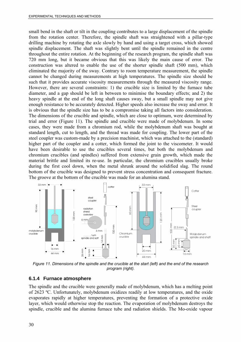
EXPERIMENTAL TECHNIQUES AND METHODS
small bend in the shaft or tilt in the coupling contributes to a large displacement of the spindle from the rotation center. Therefore, the spindle shaft was straightened with a pillar-type drilling machine by rotating the axle slowly by hand and using a target cross, which showed spindle displacement. The shaft was slightly bent until the spindle remained in the centre throughout the entire rotation. At the beginning of the research program, the spindle shaft was 720 mm long, but it became obvious that this was likely the main cause of error. The construction was altered to enable the use of the shorter spindle shaft (500 mm), which eliminated the majority of the sway. Contrary to room temperature measurement, the spindle cannot be changed during measurements at high temperatures. The spindle size should be such that it provides accurate viscosity measurements through the measured viscosity range. However, there are several constraints: 1) the crucible size is limited by the furnace tube diameter, and a gap should be left in between to minimise the boundary effects; and 2) the heavy spindle at the end of the long shaft causes sway, but a small spindle may not give enough resistance to be accurately detected. Higher speeds also increase the sway and error. It is obvious that the spindle size has to be a compromise taking all factors into consideration. The dimensions of the crucible and spindle, which are close to optimum, were determined by trial and error (Figure 11). The spindle and crucible were made of molybdenum. In some cases, they were made from a chromium rod, while the molybdenum shaft was bought at standard length, cut to length, and the thread was made for coupling. The lower part of the steel coupler was custom-made by a precision machinist, which was attached to the (standard) higher part of the coupler and a cotter, which formed the joint to the viscometer. It would have been desirable to use the crucibles several times, but both the molybdenum and chromium crucibles (and spindles) suffered from extensive grain growth, which made the material brittle and limited its re-use. In particular, the chromium crucibles usually broke during the first cool down, when the metal shrunk around the solidified slag. The round bottom of the crucible was designed to prevent stress concentration and consequent fracture. The groove at the bottom of the crucible was made for an alumina stand.
Figure 11. Dimensions of the spindle and the crucible at the start (left) and the end of the research
program (right).
6.1.4 Furnace atmosphere The spindle and the crucible were generally made of molybdenum, which has a melting point of 2623 ºC. Unfortunately, molybdenum oxidizes readily at low temperatures, and the oxide evaporates rapidly at higher temperatures, preventing the formation of a protective oxide layer, which would otherwise stop the reaction. The evaporation of molybdenum destroys the spindle, crucible and the alumina furnace tube and radiation shields. The Mo-oxide vapour
30
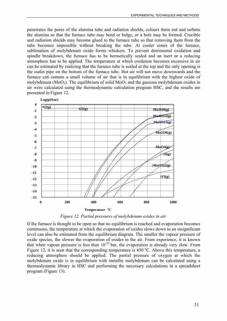
EXPERIMENTAL TECHNIQUES AND METHODS
penetrates the pores of the alumina tube and radiation shields, colours them red and softens the alumina so that the furnace tube may bend or bulge, or a hole may be formed. Crucible and radiation shields may become glued to the furnace tube so that removing them from the tube becomes impossible without breaking the tube. At cooler zones of the furnace, sublimation of molybdenum oxide forms whiskers. To prevent detrimental oxidation and spindle breakdown, the furnace has to be hermetically sealed and an inert or a reducing atmosphere has to be applied. The temperature at which oxidation becomes excessive in air can be estimated by realizing that the furnace tube is sealed at the top and the only opening is the outlet pipe on the bottom of the furnace tube. Hot air will not move downwards and the furnace can contain a small volume of air that is in equilibrium with the highest oxide of molybdenum (MoO3). The equilibrium of solid MoO3 and the gaseous molybdenum oxides in air were calculated using the thermodynamic calculation program HSC, and the results are presented in Figure 12.
0 200 400 600 800 1000-15
-14
-13
-12
-11
-10
-9
-8
-7
-6
-5
-4
-3
-2
-1
0
ºC
Log(pi/bar)
Temperature
N2(g) O2(g) Mo3O9(g)
Mo2O6(g)
Mo4O12(g)
MoO3(g)
Mo5O15(g)
O(g)
(MoO3)2(g)
O3(g)
Figure 12. Partial pressures of molybdenum oxides in air.
If the furnace is thought to be open so that no equilibrium is reached and evaporation becomes continuous, the temperature at which the evaporation of oxides slows down to an insignificant level can also be estimated from the equilibrium diagram. The smaller the vapour pressure of oxide species, the slower the evaporation of oxides in the air. From experience, it is known that when vapour pressure is less than 10-10 bar, the evaporation is already very slow. From Figure 12, it is seen that the corresponding temperature is 450 ºC. Above this temperature, a reducing atmosphere should be applied. The partial pressure of oxygen at which the molybdenum oxide is in equilibrium with metallic molybdenum can be calculated using a thermodynamic library in HSC and performing the necessary calculations in a spreadsheet program (Figure 13).
31

EXPERIMENTAL TECHNIQUES AND METHODS
1.00E-50
1.00E-45
1.00E-40
1.00E-35
1.00E-30
1.00E-25
1.00E-20
1.00E-15
1.00E-10
1.00E-05
1.00E+00
0 200 400 600 800 1000 1200 1400 1600 1800 2000
Temperature (ºC)
pO2 (
bar)
Mo + O2 = MoO2
4/3Cr + O2 = 2/3Cr2O3
aCr2O3=0.1aCr2O3=0.2aCr2O3=0.5aCr2O3=1.0
Figure 13. Partial pressure of oxygen and temperature at which molybdenum and chromium are in
equilibrium with their oxides.
The partial pressure of oxygen should be below the equilibrium line (Mo+O2 = MoO2) to avoid oxidation. Equilibrium calculation has also been performed for chromium because a part of the present study also concentrates on chromium containing slags at relatively high oxygen partial pressure (Article II in the appendices). The partial pressure of oxygen should be below the molybdenum equilibrium line (Mo+O2 = MoO2) to avoid oxidation, but above the chromium equilibrium line (4/3Cr+O2 = 2/3Cr2O3) to avoid the reduction of chromium oxide in the slag to chrome metal. Unfortunately, the required partial oxygen pressures are so small that they are impossible to obtain by using pure inert gas. Even the most pure commercial argon has much higher impurity levels of oxygen. One way to solve this problem is to use a mixture of carbon monoxide (CO) and carbon dioxide (CO2). Oxygen partial pressure can be calculated from a reaction equation (CO+½O2 =CO2), and equilibrium with molybdenum as well as carbon can be calculated. In Figure 14, it is seen that the mixture with a CO2/CO ratio below 1/10 can be used for the measurement of Cr2O3 containing slags in the molybdenum crucible. Other advantages for the use of the CO2/CO mixture include the fact that gas flow rates do not need to be adjusted during warm up and cooling the furnace, and small air leaks are effectively neutralized by large amounts of carbon monoxide. Disadvantages of this system include the fact that carbon monoxide is poisonous and requires significant care to avoid leakage to the laboratory environment. The measurement arrangement was built in a closed room with good ventilation so that escaped gases were vented directly outside of the building.
32

EXPERIMENTAL TECHNIQUES AND METHODS
Figure 14. Oxidation of Mo, Cr and C in CO2/CO atmosphere at 1 bar pressure
6.1.5 Arrangement Over the span of these studies, the measurement apparatus was improved and the measurement practice was refined due to trial and error, and often after system breakdown. The three different stages of development are presented in Figure 15, Figure 16 and Figure 19.
Figure 15. The arrangement at the start of the research program, which was used to measure the
Al2O3-CaO-MgO-SiO2 slag viscosities (Article I in the appendices).
During the measurement of Al2O3-CaO-MgO-SiO2 ‘ferrochrome base slag’ (Article I), the arrangement was as presented in Figure 15. The measurement of this slag is relatively easy because all the oxides are stable and insensitive to the oxygen partial pressure. The protective gas was chosen to be a slightly reducing mixture (95% argon + 5% carbon-monoxide). In case of a leak, carbon-monoxide is capable of eliminating a portion of the oxygen in air. The gas flow was adjusted to be about 1 litre per minute. The outgoing gas was sucked in to the ventilation system. The necessary latitude of the viscometer was obtained with air-tight teflon bellows. The construction limited the length of the spindle shaft to 720 mm at the shortest
33

EXPERIMENTAL TECHNIQUES AND METHODS
distance, which decreased the measurement accuracy (6.1.3). The only radiation shield at the top end of the furnace was a metal ring, which adversely affected the furnace’s temperature gradient. The lower radiation shields were made from molybdenum sheets, which became brittle after hot furnace use and often broke during crucible removal.
Figure 16. The arrangement for determining the viscosities of CaO-CrOx-SiO2 under high oxygen
partial pressure (Article II).
For measurements on the CaO-CrOx-SiO2 slag at a relatively high oxygen partial pressure (Article II, 6.1.4), the construction was equipped with a gas flow system designed so that gas bottles could be changed during the measurement while the furnace was hot. This system enables the use of a gas bottle until it is practically empty. It is also possible to use pure argon below the slag melting point and change to a CO/CO2 mixture at the measurement temperature. The furnace atmosphere is controlled by adjusting gas flow rates with gas flow controllers. The flow controllers used here are Brooks PC8842 and PC8845 with needle valve sizes 1 and 4, correspondingly. These valves are designed to control flows when downstream pressure is constant (in this case, normal air pressure) and upstream pressure is variable.
Figure 17. Flow rate determination with a soap bubble flow meter.
34
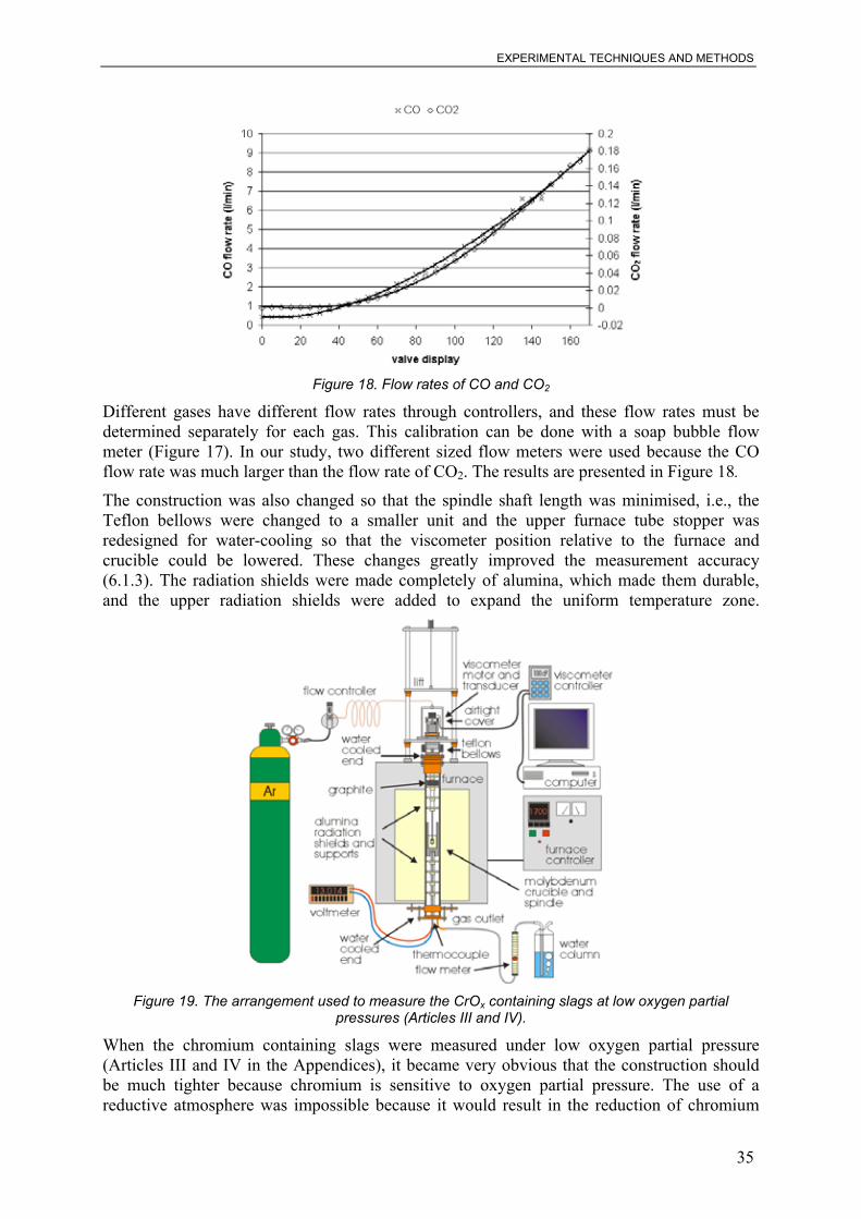
EXPERIMENTAL TECHNIQUES AND METHODS
Figure 18. Flow rates of CO and CO2
Different gases have different flow rates through controllers, and these flow rates must be determined separately for each gas. This calibration can be done with a soap bubble flow meter (Figure 17). In our study, two different sized flow meters were used because the CO flow rate was much larger than the flow rate of CO2. The results are presented in Figure 18.
The construction was also changed so that the spindle shaft length was minimised, i.e., the Teflon bellows were changed to a smaller unit and the upper furnace tube stopper was redesigned for water-cooling so that the viscometer position relative to the furnace and crucible could be lowered. These changes greatly improved the measurement accuracy (6.1.3). The radiation shields were made completely of alumina, which made them durable, and the upper radiation shields were added to expand the uniform temperature zone.
Figure 19. The arrangement used to measure the CrOx containing slags at low oxygen partial
pressures (Articles III and IV).
When the chromium containing slags were measured under low oxygen partial pressure (Articles III and IV in the Appendices), it became very obvious that the construction should be much tighter because chromium is sensitive to oxygen partial pressure. The use of a reductive atmosphere was impossible because it would result in the reduction of chromium
35
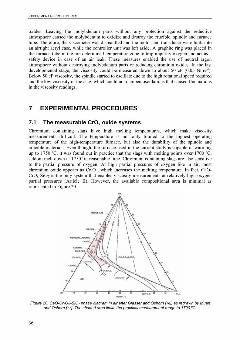
EXPERIMENTAL PROCEDURES
oxides. Leaving the molybdenum parts without any protection against the reductive atmosphere caused the molybdenum to oxidize and destroy the crucible, spindle and furnace tube. Therefore, the viscometer was dismantled and the motor and transducer were built into an airtight acryl case, while the controller unit was left aside. A graphite ring was placed in the furnace tube in the pre-determined temperature zone to trap impurity oxygen and act as a safety device in case of an air leak. These measures enabled the use of neutral argon atmosphere without destroying molybdenum parts or reducing chromium oxides. In the last developmental stage, the viscosity could be measured down to about 50 cP (0.05 Nm/s2). Below 50 cP viscosity, the spindle started to oscillate due to the high rotational speed required and the low viscosity of the slag, which could not dampen oscillations that caused fluctuations in the viscosity readings.
7 EXPERIMENTAL PROCEDURES
7.1 The measurable CrOx oxide systems Chromium containing slags have high melting temperatures, which make viscosity measurements difficult. The temperature is not only limited to the highest operating temperature of the high-temperature furnace, but also the durability of the spindle and crucible materials. Even though, the furnace used in the current study is capable of warming up to 1750 ºC, it was found out in practice that the slags with melting points over 1700 ºC, seldom melt down at 1750º in reasonable time. Chromium containing slags are also sensitive to the partial pressure of oxygen. At high partial pressures of oxygen like in air, most chromium oxide appears as Cr2O3, which increases the melting temperature. In fact, CaO-CrOx-SiO2 is the only system that enables viscosity measurements at relatively high oxygen partial pressures (Article II). However, the available compositional area is minimal as represented in Figure 20.
Figure 20. CaO-Cr2O3 -SiO2 phase diagram in air after Glasser and Osborn [76], as redrawn by Muan
and Osborn [77]. The shaded area limits the practical measurement range to 1700 ºC.
36

EXPERIMENTAL PROCEDURES
A reducing atmosphere increases the amount of CrO relative to Cr2O3, but if the atmosphere is constantly reducing, all the chromium oxide is reduced to metallic chromium. A controlled atmosphere can be obtained by equilibrating the slag with metallic chromium, either by using a chromium crucible (and spindle) or by putting chromium grains in the bottom of the molybdenum crucible. Thus, the system is fixed relative to metallic chromium, and the proportion of CrO is the highest possible, which is also the case in FeCr and stainless steel production where the slag is in contact with molten metal. Consequently, the melting point is the lowest possible. The effect of using chromium equilibrated slag can be seen in a CaO-CrOx-SiO2 phase diagram in equilibrium with metallic chromium. Now, the 1700 ºC liquidus has been extended across the centre of the phase diagram, which enables a more profound study of viscosity (Figure 21).
Figure 21. CaO-CrOx -SiO2 phase diagram in equilibrium with metallic chromium [78].
Making measurements in equilibrium with metallic chromium enables several more slag systems to be measured, such as CrOx-SiO2, CrOx-MgO-SiO2, Al2O3-CrOx-SiO2 and Al2O3-CrOx-MgO-SiO2, as represented in Figure 22, Figure 23, Figure 24 and Figure 25, respectively. The phase diagram of the CaO-CrOx-MgO-SiO2 and Al2O3-CaO-CrOx-SiO2 systems in equilibrium with metallic chromium were not observed in the literature, but they are expected to be measurable. The fewer the oxide components there are in the slag, the easier it is to see the effect of a particular oxide on viscosity. Therefore, it would be important to know the viscosities of binary and ternary slag systems. However, fewer components results in a smaller available measurement area usually. Therefore, measurements were restricted to the pseudo-ternary slag systems and one pseudo-quaternary system, namely Al2O3-CrOx-MgO-SiO2.
37

EXPERIMENTAL PROCEDURES
Figure 22. CrOx-SiO2 phase diagram in equilibrium with metallic chromium [79].
Figure 23. CrOx-MgO-SiO2 phase diagram in equilibrium with metallic chromium as reported by Muan
[80], according to the results of Collins et. al. [81]. Figure adopted from Slag Atlas [18].
38

EXPERIMENTAL PROCEDURES
Figure 24. Al2O3-CaO-CrOx under mildly reducing conditions after Kaiser et al. Figure adopted from
Slag Atlas [18].
Figure 25. Al2O3-CrOx–MgO-SiO2 in equilibrium with metallic chromium (MgO+Al2O3 weight ratio
MgO/Al2O3 =2) [82].
39
EXPERIMENTAL PROCEDURES
7.2 Sample preparation The most important aim in preparing samples is to ensure that the slag will melt and form homogenous liquids when heated. If the sample does not melt, viscosity cannot be measured. The sample state cannot be inspected in a closed furnace, and there is also the threat that the spindle shaft will bend or break when immersed into the crucible if the slag has not melted. Second, the oxide powders should be treated such that required amounts fit into the crucible. There must be enough molten slag so the spindle is immersed to the required depth and is fully covered with liquid slag. Different oxides have different densities, and finer oxide grains require more volume than coarse grains. The third important aim is to prepare oxides to form a slag, which is as close to the target composition as possible. This is achieved by using oxides which have little impurities, heat treating oxides before weighing at 400 ºC to remove moisture and crystalline water, and heat carbide forming substances at 800 ºC to remove carbon. Finally, the oxides must be weighed carefully in a micro-scale, blended and mixed in a powder mixing machine to achieve total mixing of different oxide species. The slag is analysed after the viscosity measurement, and the results are used for the construction of mathematical viscosity models, which enable the calculation of viscosity at the exact composition and temperature, even though the real composition of the sample differs from the desired target composition. These two important aims may be achieved by similar methods. In practice, it is best to use a method requiring minimal effort. The possible methods are listed here from the least to the most laborious effort:
If the slag has a low melting point and high density, the crucible can be filled with well-mixed oxide powder with slight treading. Good mixing breaks up agglomerates and helps melt down the material. 100 grams is usually enough for a crucible of the size in Figure 11.
If an oxide mixture has a lower density and 100 g will not fit in to the crucible, it can be pressed into pellets in a hydraulic press. This also brings the oxide grains closer to each other, which also helps meltdown. This method was used for slag samples in Articles 3 and 4 in the Appendices.
It is also possible to pre-melt an oxide mixture in a separate graphite crucible in a vacuum induction furnace, which can be heated to higher temperatures relative to the resistance furnace. After the slag has been melted once, the second meltdown is easier. After pre-melting, the slag is poured on the metal plate, where it immediately solidifies, forming a glass like microstructure. Fast cooling is necessary because it prevents equilibrium freezing along the solidus and liquidus, which would cause compositional segregation. The solidified slag is then crushed and mixed. Usually, when the oxide species reacted, the volume shrank and it easily fit in the measurement crucible. It is better to fill the vacuum furnace with argon so the volatile oxides are not so easily evaporated. Excessively high temperatures should also be avoided for similar reasons. Certain oxides like Fe2O3 and Cr2O3 can react with the graphite crucible, so this method cannot be used. Even SiO2 (SiO) will evaporate at high temperatures, especially if carbon is present, which consequently changes the composition. This method was used for the Al2O3-CaO-MgO-SiO2 slag in Article I in the appendices.
Fe2O3 and Cr2O3 containing slags can also be pre-melted directly in the measurement crucible of a vacuum induction furnace at argon atmosphere. This method was used for a CaO-CrOx-SiO2 slag in Article II because the melt down proved to be extremely difficult. Pre-melting had to be performed in a more powerful induction furnace because the molybdenum crucible consumed part of the furnace output. Unfortunately, furnace control was very difficult and SiO started to evaporate intensively close to the melting point, so that the mixture started to boil over, changed the composition, or even reduced the amount of slag so that measuring the viscosity was no longer possible. Because of the compositional segregation during
40
EXPERIMENTAL PROCEDURES
solidification, the samples should be homogenized at high temperature long enough before the first measurement (Ch.7.3). The successful samples were used for viscosity measurement in Article II.
7.3 Viscosity measurement procedure The crucible was filled with 100 - 110 g of a slag and placed into the furnace. The spindle was attached to a viscometer and the viscometer was let to ‘auto-zero’, the furnace was closed, and free rotation of the spindle, flow of cooling water and protective gas were verified. It is possible to save gas by waiting to open the gas valve until the furnace reaches 400 ºC. The furnace was programmed to heat to a maximum temperature of 1750 ºC at a rate of four degrees per minute. This takes approximately seven hours. When maximum temperature was reached, the furnace was maintained at maximum temperature for one to three hours to stabilize the temperature variations and ensure that high melting point slags formed homogenous liquids. During that time, the spindle was immersed into the molten slag and heated with the slag. Care must be taken when the spindle is immersed because if the slag has not melted, the spindle shaft and the viscometer bearings might break. The spindle was rotated while slowly lowering the spindle, and the torque reading was followed constantly. First, the torque reading (as well as viscosity) should be zero. When the spindle touched the slag, the torque reading began to rise. If the slag melted, the torque reading increased slowly as the spindle sank into the slag. However, if the torque reading increased rapidly and went out of zone, this suggested that the slag had not melted. After temperature stabilization, the first viscosity measurement was taken using several rotational speeds, but not speeds that exceeded 60 RPM, and not speeds in which the torque was less than 10%, because higher speeds increase the sway and the error became significant. Low resistance (torque-%) did not give accurate readings either. The furnace was programmed to cool down in steps (50 ºC with lower- and 20 ºC with higher- melting point slags). The temperature stabilized for 30 minutes after every 50 ºC temperature drop and 20 minutes after every 20 ºC before new measurements were taken, while using several rotational speeds. After measurements, the furnace was heated to help the slag drain from the spindle when the spindle was removed from the slag. The furnace was then cooled to room temperature, which took even more time than heating. At high temperatures, the furnace cooled quickly and power was necessary to decrease the cooling rate. When the temperature was near 1000 ºC, the cooling rate decreased so that power was no longer necessary. The protective gas flow was stopped when the temperature reached 400 ºC. In the first experiments, the viscosity was measured both during the cooling and heating cycles. It was believed that the viscosity would show hysteresis because of temperature differences during the cycles. However, the hysteresis behaviour was far too strong for the small temperature variations. It was concluded that irrevocable compositional segregation occurred during the cooling cycle, where the solid phase collected on the sides of the crucible and did not dissolve the liquid during heating. An example of such an experiment is shown in Figure 26.
41

EXPERIMENTAL PROCEDURES
0
500
1000
1500
2000
2500
3000
3500
4000
1450 1500 1550 1600 1650 1700 1750
Temperature (ºC)
Visc
osity
(cP)
Figure 26. Basic behaviour of viscosity during cooling and heating cycles. The first measurement was
taken at the highest temperature following the cooling cycle.
During temperature stabilization time at high temperature, the slag forms a homogeneous liquid. When the first measurements were taken, the slag was in a homogeneous liquid state and the viscosity followed the Arrhenius equation. When the temperature decreased to the melting (liquidus) point, a solid phase started to segregate from the melt on top of the slag, on the walls and the bottom of the crucible, according to the temperature gradient. This solid phase had a different composition relative to the remaining liquid phase, as can be verified from a suitable phase diagram. When the amount of the solid phase increased so much that it touched the spindle, the viscosity seemed to increase rapidly, as schematically represented in Figure 27.
Figure 27. Schematic illustration of solidification in a crucible during the cooling period.
Consequently, viscosity may seem to increase smoothly well below the liquidus temperature, until the solid phase finally hinders the spindle movement. When the temperature is increased again, the viscosity is much higher than during the preceding cooling cycle. This occurs because the solid phase, which might have a very high melting point, does not melt again in a reasonable period of time. Melting would need compositional homogenisation, which occurs by diffusion and requires time. Nevertheless, the measured viscosity below the melting point (liquidus) is not the viscosity of the same slag above the liquidus, because the remaining liquid slag has diluted components and the composition was altered. Therefore, the only
42
EXPERIMENTAL PROCEDURES
“right” viscosity values can be obtained at temperatures above the melting point during the first cooling cycle, when no compositional segregation has occurred. The existence of the remaining solid phase at temperatures above the liquidus has also been proven by adjusting the spindle height in the slag. At the normal position, the viscosity was very high, but at a position a few millimetres above the normal level, the viscosity decreased to very low values. At higher positions, the viscosity seemed to rise again, which was taken as proof of a solid slag cover. In one trial, the spindle was raised several times up and down through the solid cover. This was thought to break the solid lid, which, as a heavier phase, was thought to sink to the bottom of the crucible. The spindle was then removed from the slag and the furnace was able to cool. The crucible was split in two halves, and an optical examination of the longitudinal section showed a darker phase at the bottom of the crucible (Figure 28). During splitting the crucible by sawing and emptying the used crucibles by drilling, it was observed that the slag on the bottom of the crucible was harder than the slag on the top. Compositional analysis was made by SEM-EDS, which also supported compositional segregation. The last solidified liquid was collected in the centre of the crucible, i.e., in the middle of the longitudinal section. The bottom phase differed from the top, because it solidified earlier (as the first solidified top was broken by the spindle and sank to the bottom).
Figure 28. Scanned image of a longitudinal section of the slag, and compositions from top to bottom.
Image contrast was enhanced.
For this reason, the concentric cylinder methods cannot be used to determine the melting points nor to verify the corresponding phase diagrams.
7.4 Sample analysis As explained in the previous chapter, compositional segregation occurs during solidification. The sample should be taken so that it best represents the total composition of the slag, which means emptying the whole crucible for sample analysis. At the beginning of the program, the crucibles were emptied by percussion drill, which was extremely arduous (Article I). Later, the crucibles were emptied by using a water cooled diamond (cylinder) drill, which had a size close to the inner diameter of the crucible. A solid piece of slag from the crucible was crushed in an eccentric mill and used for analysis. The total chromium content as well as Al2O3, CaO, MgO and SiO2 were analysed by an x-ray spectrometer, except for the samples with more than 45% CrOx, which were analysed by the wet-chemical method. The amount of “CrO” was measured by wet-chemical analysis. The resulting value was subtracted from the total CrOx content to determine the amount of Cr2O3. The main procedure of the wet-chemical analysis of CrO begins with dissolution of the slag in HCl in an inert gas atmosphere in the presence of
43

SUMMARY OF THE PUBLICATIONS
Fe3+ chloride (FeCl3). Cr2+ is then oxidized with 3-valent iron to Cr3+, and the same molar amount of Fe3+ is reduced to Fe2+:
++++ +=+ 2332 FeCrFeCr (129)
The quantity of Fe2+ ions can then be determined by titration with standard permanganate solution:
OHMnFeHMnOFe 223
42 4585 ++=++ +++−+ (130)
The wet-chemical analysis was performed for slowly cooled slag samples. During the cooling period, some of the CrO decomposes to Cr2O3 and Cr metal, but had no effect on wet-chemical analysis results, since the reducing power remains similar:
FeOOCrOFeCrO 33 3223
3223 +=+ (131)
323 OCrCrCrO += (132)
FeOOCrOFeOCrCr 33223
3223
32 +=++ (133)
According to previous studies [1,83], the effect of temperature on the distribution of di- and trivalent chromium is relatively small, and was thus ignored.
8 SUMMARY OF THE PUBLICATIONS
8.1 Experimental study of the viscosities of selected CaO-MgO-Al2O3-SiO2 slags and application of the Iida model
The selected compositions in the first article are in the same compositional area relative to the ‘base slag’ used in ferrochromium production. In FeCr-production, the base slag dissolves already partly reduced solid ferrochrome concentrate (lumpy ore or pellets). Carbon (coke) tends to react with oxygen atoms in the slag, forming carbon monoxide (CO). Removal of oxygen ions from an oxide results in metal formation. In the FeCr process, slag iron is the least stable oxide and chromium oxide is the next least stable. Thus, iron will preferentially precipitate out of slag and coalesce into metal droplets. At temperatures over 1500 °C, chromium oxide can be reduced into metallic chromium, which is dissolved into iron. The ferrochrome droplets are separated out of slag under gravitational force due to the weight difference of slag and metal, and they form a metal bath in the bottom of the furnace. It is obvious that viscosity plays an important role for each of the process steps, and for the overall process efficiency. The base slag typically has low basicity with fairly high Al2O3, MgO and SiO2 contents, but low CaO. The liquidus temperatures are high and vary from about 1580 °C to over 1700 °C. There are plenty of measured viscosity data available in the Al2O3-CaO2-MgO-SiO2 system, but none were performed near the base slag region in the ferrochromium process (Outokumpu). The viscosity results of this study can be used for re-optimising the available viscosity models for better applicability, with respect to the compositional range of ferrochromium process slag. The modified Iida model was also applied to the measured viscosities. The ‘modification’ model parameter for Al2O3 (α*Al2O3) was determined using the measured viscosities of the present study, while all other parameters were ‘classical’ Iida parameters, which were based on the characteristic properties of the elements. The model accurately reproduced the viscosities within the composition range in question.
44

SUMMARY OF THE PUBLICATIONS
8.2 Viscosity of CaO-CrOx-SiO2 slags in relatively high oxygen partial pressure atmosphere
Because of the high melting temperatures of chromium containing slags, viscosity could only be measured using the available apparatus in neutral or oxidizing atmosphere for CaO-CrOx-SiO2. The compositional area in which the measurements could be made proved to be even smaller than the indicated phase diagram. Several measurement attempts failed, with slags containing more than 10% Cr2O3, in a narrow peninsula on the phase diagram extending the 1700 °C liquidus close to 20 weight-% of Cr2O3 (Figure 20, Ch.7.1) The oxygen partial pressure was adjusted using a mixture of carbon monoxide (CO) and carbon dioxide (CO2) to be reducing relative to Mo+O2=MoO2 equilibrium, but oxidizing concerning Cr+½O2=CrO and 2CrO+½O2=Cr2O3 equilibria. An effort was made to inspect the effect of adjusting the oxygen partial pressure during the trial by changing the ratio of CO and CO2 flow rates, but no result was observed in a reasonable time frame. The Iida model was applied for the measured viscosities. The previously undefined specific coefficient αCrO and the hypothetical viscosity of pure oxide μ0CrO were determined solely on theoretical bases. The Iida model showed very good consistency with the measured values, taking into account that no adjustment was made to the model parameters using the results of the present study. On the other hand, the chromium content in the measured slags was low, and thus the effect on viscosity was small.
8.3 Viscosity of SiO2-CaO-CrOx slags in contact with metallic chromium and application of the Iida model
Equilibrating the slag with metallic chromium decreases the partial pressure of oxygen, which was proved to increase the proportion of CrO relative to Cr2O3, and decreased the melting temperatures as well. In a reducing atmosphere, the SiO2-CaO-CrOx system offers the widest compositional area where the viscosity measurements may be performed. The viscosities were measured up to 60 wt%CrOx concentration. The distribution of CrOx into CrO and Cr2O3 was determined by a regression analysis based on the previous study on activities by Y. Xiao. The Iida model with ‘fundamental’ α-parameters based on the physical properties of elements was not consistent with the measured values of the high chromium containing slags. By adjusting the α-parameters for CrO and Cr2O3 , good consistency was found. In the Iida model, the α-parameter can be considered a measure of the characteristic basicity of an oxide. The new adjusted parameters indicated that CrO was stronger and Cr2O3 was a much stronger basic oxide relative to the indicated ‘fundamental’ α-parameters.
8.4 Experimental study and modelling of viscosity of chromium containing slags
Equilibrating the CrOx containing slag with chromium metal extends the possibility of viscosity measurements in several oxide systems. The slag systems CrOx-SiO2, CrOx-MgO-SiO2, Al2O3-CrOx-MgO-SiO2, CaO-CrOx-MgO-SiO2 and Al2O3-CaO-CrOx were explored and viscosities were measured. The results, including the previously measured CrOx-CaO-SiO2 system, were used to expand the modified Urbain model and include CrO and Cr2O3, in addition to oxides which already existed in the model, i.e., Al2O3, CaO, FeO and SiO2. A literature review was conducted to gather viscosity data on MgO containing slags to include MgO into the model. The modified Urbain model gave a reasonable fit with the measured viscosity values, and can be applied in a wide variety of oxide systems over large compositional areas.
45

RESULTS AND ERROR ANALYSIS
8.5 Assessment of viscosity of slags in ferrochromium process A neural network method was applied to the viscosity data measured during the course of this study combined with the literature review data of the unary, binary, ternary and quaternary
sub-systems of the Al2O3-CaO-CrO-CrO1.5-MgO-SiO2 slag. The model was used to estimate the effect of chromium oxides on the viscosities of slags as well as to predict viscosities in typical FeCr process slags. The neural network approach proved to be a practical tool in predicting the viscosities of multi-component slags containing chromium.
9 RESULTS AND ERROR ANALYSIS The viscosity measurements failed frequently because the slag could not be melted, the viscosity arrangement broke due to an air leak or the materials could not stand the high temperatures. A number of failed experiments were not recorded, but roughly 50% of the measurements were successful, and the results of those experiments are shown in Table 2. The same results are presented in the five articles in the appendices. The compositions of the CaO-CrOx-SiO2 in equilibrium with metallic chromium (slags 21-34) are target compositions, and the distribution of total (target) chromium content CrOx into CrO and Cr2O3 was estimated by regression analysis based on Y.Xiao’s work [1]. Table 2. Results of the viscosity measurements. The compositions of slags 21-34 are target compositions, for which the distribution of total chromium CrOx into CrO and Cr2O3 was estimated by regression analysis. All other compositions were analysed after the measurements.
CrO Cr2O3 Al2O3 CaO MgO SiO2 Log η (P), T(K) temp. Range (°C)
1 51.91 48.09 8724.39.7443−
T 1460-1750
2 54.5 45.5 1227.41.7989−
T 1440-1750
3 37.4 62.6 0138.43.8890−
T 1550-1750
4 24.6 24.0 51.4 0672.43.7971−
T 1440-1750
5 23.46 10.09 25.3 41.13 4364.47.9655−
T 1580-1750
6 27.05 10.21 19.57 43.16 2274.44.8987−
T 1590-1750
7 23.02 2.20 34.43 40.35 0039.44.8345−
T 1620-1750
8iii 29.48 2.03 27.52 40.97 323.2656949
−T
1640-1750
9 28.96 1.84 27.53 41.66 2285.39.7318−
T 1640-1750
10 20.30 10.32 31.45 37.92 4987.47.9181−
T 1660-1750
11 23.65 10.86 25.08 40.41 2809.44.8982−
T 1670-1750
12 22.22 2.08 39.25 36.45 2775.41.8554−
T 1690-1750
13 26,10 19,34 29,38 25,18 3648.44.8660−
T 1690-1750
iii Slag 8 was melted several times in order to test the repeatability of the viscosity measurements. The repeatability proved to be very good, but due to the compositional segregation in the crucible, the result was not representative for the given composition.
46

RESULTS AND ERROR ANALYSIS
CrO Cr2O3 Al2O3 CaO MgO SiO2 Log η (P), T(K) temp. Range (°C)
14 24.85 19.25 15.58 40.33 821.30.8498−
T1550-1750
15 4.41 4.54 52.46 38.62 2853.36026−
T1660-1750
16 1.60 1.58 52.84 43.98 9934.33.7479−
T1570-1750
17 2.16 0.34 51.75 45.75 7775.32.7176−
T1470-1750
18 3.00 1.60 50.26 45.14 1689.47.8063−
T1470-1750
19 1.41 0.82 47.82 49.95 9328.34.7931−
T1480-1750
20 2.22 0.27 45.91 51.61 9372.31.8051−
T1490-1750
21 1.83 0.53 37.77 59.88 8021.36.8587−
T1500-1750
22 40 60 1266.49.8612−
T1440-1750
23 9.77 0.23 55 55 2288.48.8658−
T1440-1750
24 17.88 2.12 50 50 0721.48067−
T1450-1750
25 23.61 6.39 45 45 7161.36.6921−
T1500-1750
26 27.27 12.73 40 40 5109.32.6237−
T1550-1750
27 28.96 21.04 35 35 3615.47698−
T1600-1750
28 28.84 31.16 30 30 0355.55.8521−
T1550-1750
29 50 50 5577.36.6694−
T1350-1750
30 9.05 0.95 45 45 3057.32.6093−
T1500-1750
31 15.82 4.18 40 40 3927.42.7926−
T1500-1750
32 20.29 9.71 35 35 2864.38.5662−
T1500-1750
33 22.42 17.58 30 30 1908.41.7275−
T1550-1750
34 22.22 27.78 25 25 6443.42.7908−
T1600-1750
35 19.65 40.35 20 20 0929.59.8686−
T1600-1750
36 32.62 33.08 34.30 5826.49.8353−
T1480-1750
37 1.40 18.37 27.05 53.18 056.57.9948−
T1500-1750
38 3.10 26.24 24.31 46.36 9907.510984−
T1400-1750
39 3.24 37.31 13.93 45.53 7385.510717−
T1430-1750
40 1.14 18.17 14.78 10.74 55.18 0937.48.9361−
T1600-1750
41 2.52 25.51 9.73 9.32 52.93 5761.42.996.9−
T1600-1750
42 4.08 33.63 7.71 7.30 47.28 6094.511437−
T1630-1750
43 2.17 6.63 23.23 20.90 47.07 0557.43.7754−
T1445-1750
44 5.04 12.18 21.17 18.85 42.75 1844.59513−
T1445-1750
47

RESULTS AND ERROR ANALYSIS
CrO Cr2O3 Al2O3 CaO MgO SiO2 Log η (P), T(K) temp. Range (°C)
45 8.12 12.46 21.48 16.61 41.33 7736.1020501−
T1550-1750
46 15.92 19.96 16.80 14.84 32.47 9583.1122652−
T1590-1750
47 22.15 26.23 12.47 12.06 27.09 Not melted
48 2.86 7.54 38.69 50.91 2619.1019557−
T1680-1750
The validity of the viscosity measurements was verified at room temperature by calibrating the construction for each spindle with at least three silicon oils (50 cP, 100 cP, 500 cP, and sometimes 5000 cP), and at high temperatures using a reference slag with a previously measured composition (without chromium). At the beginning of this research program, the first sample (Slag 8) was measured several times to test the repeatability of the viscosity measurements. The measurements were made with the same crucible and slag, but with a different spindle. The separate measurements agreed remarkably well with the viscosity values as presented in Figure 29. The largest difference above the melting point was about 5%. Later, it was noticed that irreversible compositional segregation occurred during solidification. Therefore, the sample and trial were reproduced (Slag 9).
Figure 29. Repeatability of the viscosity measurements
A few examples of the validity tests are shown in Figures 30, 31 and 32. The compositions were selected to provide a reference point to compare the addition of chromium. The comparisons show a very good resemblance, although not all of the comparisons were as assertive. The viscosity of Slag 22 (40 wt% CaO-SiO2) and Slag 29 (50 wt%CaO-SiO2) were somewhat lower compared to Bockris´ results [84], although the shape of the measured viscosity curve was exactly same.
48

RESULTS AND ERROR ANALYSIS
Figure 30. CaO-SiO2 system. Comparison of viscosity values with data provided by Bockris and Lowe
[84].
Figure 31. Comparison of slags 2, 3 and 4 to the data found in literature [84,85,86].
49
RESULTS AND ERROR ANALYSIS
Figure 32. Chromium containing slags 17 and 18 compared to the slag viscosity measured by B.
Vidacak. [87]
It is very difficult to estimate the error margins quantitatively. This would require the use of a reference material, in which viscosity would be known, and the measurements for this material would be repeated multiple times to solve the standard deviation. Furthermore, measurement of the reference material would be easier than the measurement of a chromium containing slag, which is sensitive to measurement conditions. The various sources of error are discussed qualitatively in the following:
1. The error of the measurement device (Brookfield LVDV 2+) is caused by the calibrated spring, which is ±1% of the full range viscosity reading and is dependent on the particular spindle and rotational speed. This uncertainty cannot be avoided and must be summarized for other uncertainties.
2. Misinterpretation of the viscosity reading arises from the toss of viscosity display. This can be minimised by calculating an average between several measurements or by noting the minimum and the maximum readings and calculating an average.
3. Additional error originated from the determination of the system constant (SMC). This can be due to dirty or old standard calibration fluid, and to the accuracy of the temperature control at which the determination must be performed (25 ºC). These effects can be minimised by checking the calibration oil before its use, i.e., measuring the viscosity with a standard spindle, and by being careful with the temperature control.
4. Although the SMC has been successfully determined, the actual measurement may have been changed so that the corresponding SMC should be different. The amount of slag compared to the amount of calibration oil may be different. The dimensions of the spindle and crucible change are due to thermal expansion. The position of the spindle in the crucible may change because the crucible is not exactly in the same position (for example if the furnace tube has been bent). These effects can be minimised by being careful and checking the SMC every time a change in measurement settings is suspected.
50
DISCUSSION
5. The increasing sway of the spindle at higher rotational speeds promotes additional viscometer resistance. This effect shows that when the SMC constant is determined, i.e., the SMC at low speed (and more viscous calibration oil) seems to be different relative to the SMC at high speeds (and a less viscous calibration oil). The gap between these two SMC values can be minimised by reducing the spindle mass using a straighter shaft and ensuring that the connection with the spindle and shaft is as straight as possible. It was observed that the length of the spindle shaft and the mass of the spindle has a great effect on the accuracy of the SMC constant. The shorter (more rigid) shaft and lighter spindle gave a narrower difference in SMC values.
6. The exactness of temperature during measurement is another source of error. The thermocouple was placed under the crucible c.a. 10 mm below the slag, therefore for a steep temperature gradient, the temperature is not exactly similar to that of the slag. Also, the thermocouple may age and give incorrect readings. The thermocouple should be checked from time to time.
7. Errors in compositional analysis. The crucible should be totally emptied to obtain a representative sample. Smaller samples taken from the centre of the crucible may not include the compositions which have been segregated on the sides during solidification. In particular, the wet chemical analysis of chromium is prone to errors and should be conducted with great exactness.
8. The viscometer may lose its calibration. Therefore, the calibration should be checked periodically.
Although there are many variables that might influence the accuracy of the measurement, nearly all can be controlled by careful repair of the experimental apparatus, careful determination of the SMC and careful measurement of viscosity. These all are dependent on the person conducting the experiment.
10 DISCUSSION The chromium content in a real process slag is normally relatively low due to reducing process conditions. In ferrochrome production, the chromium content in terms of Cr2O3 is about 5 wt-%, and in stainless steel production it varies from 1.5 wt-% to about 10 wt-% (Cr2O3). For practical purposes such as chromium recovery, the most interesting slags have fairly low chromium content. However, due to experimental errors in compositional analysis, temperature and viscosity measurements, it would be difficult to determine the effect of chromium addition on viscosity with such low chromium concentrations. Therefore, the effect of chromium on viscosity has to be measured using higher chromium concentrations, and the compositional range of interest between 0-10 wt% has to be interpolated from the measured values. The high chromium slags are especially valuable for the construction of the mathematical viscosity models and for defining the model parameters.
10.1 Effect of chromium oxide addition on viscosity The addition of chromium oxide decreases the viscosity but increases melting temperature. As an example, two systems are considered. The first is a CaO-CrOx-SiO2 system with the target compositions represented in Table 3 and the same compositions illustrated in the phase diagram in Figure 33, and the second is a CaO-CrOx-MgO-SiO2 system with the analysed
51

DISCUSSION
Table 3. Target compositions in the CaO-CrOx-SiO2 system.
Target compositions (weight%)
Slag CrOx CaO SiO2
1 0 40 60
2 10 35 55
3 20 30 50
4 30 25 45
5 40 20 40
6 50 15 35
7 60 10 30
Figure 33. The slag compositions in Table 3 are illustrated using a CaO-CrOx-SiO2 phase diagram in
equilibrium with metallic Cr.
compositions as represented in Table 4. Both systems were equilibrated with metallic chromium.
The measured viscosities of the CaO-CrOx-SiO2 slags are represented in Figure 34. The data points that do not fit the linear (Newtonian) trend line have been ignored because it has been assumed that the slag has begun to solidify, causing increases in the viscosity. Also, this figure shows that the more CrOx is present in the slag, the less data is acquired because of the higher melting temperatures.
52

DISCUSSION
Figure 34. Logarithm of the viscosities of CaO-CrOx-SiO2 slags versus the reciprocal of the absolute
temperature.
Plotting the viscosities of the slags against the increasing CrOx content in Figure 35 shows that small CrOx additions resulted in a relatively strong decrease in the viscosity. With increasing CrOx additions, the viscosity decrease became gradually weaker (to about 55 mol% of CrOx). However, because the ratio of CaO/SiO2 decreases when the amount of CrOx increases, the absolute viscosity decreasing effect of CrOx cannot be directly observed.
Figure 35. Effect of CrOx addition on the viscosity of CaO-SiO2 slag.
53

DISCUSSION
The effect of CrOx addition on viscosity could also be verified with CaO-CrOx-MgO-SiO2 slags. The analysed compositions are presented in Table 4. The basicity ratios of the slags are quite close to each other [(CaO+MgO)/SiO2 ≈ 1.2], which enables the viscosity comparison as presented in Figure 36.
Table 4. Analysed compositions in the CaO-CrOx-MgO-SiO2 system
CrOx CrO CrO1,5 CaO MgO SiO2 CaO+MgO
SiO2
0.00 0.00 0.00 23.22 31.51 45.27 1.21 6.49 1.74 4.75 22.57 28.25 42.69 1.19
13.09 4.14 8.95 21.08 26.11 39.73 1.19 16.04 6.76 9.28 21.69 23.33 38.94 1.16 29.14 13.73 15.41 17.57 21.59 31.70 1.24 40.83 19.82 21.00 13.53 18.21 27.44 1.16
Figure 36. The effect of CrOx addition on the viscosity of CaO-MgO-SiO2 slag
Under reducing conditions, the chromium in a slag is distributed as divalent and trivalent oxides. The divalent to trivalent oxide ratio depends on experimental conditions, which were fixed for the slags in question using metallic chromium in contact with the slag. The reaction equation can be written:
2(CrO1.5) + Cr = 3(CrO) (134)
The analysed distributions of CrOx into CrO and CrO1.5 from Table 4 are plotted in Figure 37.
54

DISCUSSION
Figure 37. Distribution of total CrOx content into CrO and CrO1.5.
10.2 The applied viscosity models The modified Iida model (Article I) was developed for the FeCr process base slag (24.6-31.5 wt% Al2O3, 1.8-19.6 wt% CaO, 17.8-38.4 wt% MgO, 25.6-41.2 wt% SiO2). The model optimisation using the measured values was only done by defining the α*-parameter for amphoteric Al2O3. The α*-parameter is dependent on basicity (Bi) and the amount of Al2O3 (WAl2O3) in the slag. The modified Iida model prediction is illustrated for a typical FeCr process base slag in Figure 38 (cross-section of an Al2O3-CaO-MgO-SiO2 slag with constant 25 wt% Al2O3 content). The dashed iso-viscosity lines are inclined from left to right, which means that for a similar effect on viscosity, more MgO than CaO has to be added to SiO2. This is logical because CaO has been reported to be a slightly stronger basic oxide. The solid iso-viscosity lines in Figure 38 have been calculated using the modified Urbain model. In this case, the lines are inclined from right to left, which would indicate that MgO is a more basic oxide than CaO, which should not be the case. Figure 38 shows that the modified Iida model and the modified Urbain model predictions become closer to each other in the CaO depleted area, whereas the deviation increases in the CaO rich area. Iida et. al. extensively applied the viscosity data measured by Machin et. al. to optimise their model [52,54], whereas Kondratiev et. al. omitted these data completely [38]. In this study, the modified Urbain model was optimised only with respect to the MgO and CrOx parameters, while the parameters for Al2O3 and CaO (and FeO) had been previously optimised. Clearly, the biggest proportion of the available viscosity data of MgO containing slag was provided by Machin et. al., and was used for MgO parameter optimisation. Therefore, it is logical that the predictions of the two models approach each other when the slag is MgO rich, but deviate when the amount of MgO decreases. However, both models accurately predict the measured viscosities of the measured FeCr-process base slags (Article I); the average deviation of the modified Iida model was 9.7%, and the modified Urbain model was slightly worse, 15% (Article IV). According to both models, the viscosity of the FeCr-process base slag is between 10-20 cPas (circled area, above the liquidus in Figure 38).
55

DISCUSSION
Figure 38. Comparison of the modified Iida model (dashed lines ----) and the modified Urbain model (continuous lines ___) predictions for the Al2O3-CaO-MgO-SiO2 slag with constant 25 wt% Al2O3 at 1700 °C. The circled area represents the compositional range of FeCr process base slag.
The effect of hypothetical pure CrO and CrO1.5 additions into FeCr process base slag is illustrated in Figure 39A and B, and in Figure 40A and B. Figure 39A was constructed using the modified Iida model (Article I) with the CrO and Cr2O3 parameters, which were determined from the valences, ionic radii of Cr2+, Cr3+ and O2- and molecular weights of CrO and Cr2O3 (Article II). However, the Iida model could not reproduce sufficiently the viscosities of slags that contain higher amounts of chromium, as was proven in the study of CaO-CrOx-SiO2 slag in contact with metallic chromium (Article III). Therefore, the αCrO and αCr2O3 parameters were optimised using measured data. The congruence between the measurements and predictions was greatly improved giving an average deviation of 13.1% for the slag system in question, but the optimised α parameters indicated that CrO and Cr2O3 were stronger basic oxides than the classical Iida definition would propose based on the characteristic physical properties of the elements (Ch.5.5). According to both approaches, CrO decreases the viscosity more than CrO1.5, and the minimum viscosities are reached close to the addition of 50 wt% to the chromium oxides. In real slag, the CrOx distributes both to divalent and trivalent oxides, which is roughly estimated here by assuming a fifty-fifty distribution, and is presented as ‘semi-dash’ lines between the pure oxides in Figure 39 and Figure 40.
56

DISCUSSION
(A) (B)
Figure 39. A) Effects of hypothetical pure CrO and CrO1.5 additions into typical FeCr process base slag (FeCr-BS) on viscosity according to the modified Iida model with classically defined α-parameters, and B) according to optimised α-parameters . The composition of the FeCr-BS was 25 wt% Al2O3-5 wt% CaO-35 wt% MgO-35 wt% SiO2 and the temperature was 1700 °C.
Figure 40A was constructed using the modified Urbain model, for which the CrO and Cr2O3 parameters were optimised using the measured viscosities of several slag systems containing chromium (Article IV). Figure 40B was constructed using Neural network computation (Article V). The formulas used in the Neural-network computation do not describe the inner structure of the silicate network like formulas used in the Iida model, the Urbain model and the other structure related viscosity models. A model, which is based on the logical description of the silicate structure, can be optimised using fewer measured data points and should be better able to predict the viscosities of compositional areas where measured data are not available. On the other hand, the model, which does not try to emulate the silicate structure like the model based on Neural-network computation, does not have the eventual weaknesses and simplified assumptions of the structure-related models. In that respect, results of the Neural-network model are ‘neutral’ or ‘clean’ and can provide self-sufficient evidence of properties such as the characteristic basicities of the oxides. At zero concentration of CrOx, the modified Urbain model deviates from the modified Iida models by the moderate amount of 1.12 cPas, which arises mainly from the applied viscosity data and the formalism of amphoteric oxides. The Neural-network model deviates 1.8 cPas from the Iida model prediction, which arises mainly from the applied optimisation data. For practical purposes, it is most interesting to know the viscosities of the slags which contain chromium less than 10 wt% and are in contact with metallic iron and chromium. In this region, the addition of a total of 10 wt% of 50% CrO-50% CrO1.5 mixture decreases the viscosity by 2 cPas in the Iida model with conventional parameters α, and by 2.87 cPas with optimised α parameters. Similarly, the addition of 10 wt% CrOx mixture decreases the viscosity by 4.87 cPas according to the modified Urbain model, and 3.62 cPas according to the Neural network model. For the CaO-CrOx-SiO2 slags measured at high oxygen partial pressure (Article II) and containing less than 9 wt% of CrOx, the Iida model and the modified Urbain model performed equally well with average deviations of 11.77% and 11.90%, respectively. The measure of
57

DISCUSSION
characteristic basicity of an oxide in the Urbain model can be considered the value of the m parameter, i.e., the lower the m-value, the more acidic the oxide, and vice versa. Even though
the m parameter for CrO was defined to be 0.75 and considerably less than 0.5 for CrO1.5, the modified Urbain model predicts that CrO1.5 decreases viscosity more effectively than CrO up to 25 wt% CrOx concentration. For viscosity predictions of real slags, this is not an issue because real slags contain a mixture of CrO and CrO1.5 oxides, and the error is counterbalanced. This also illustrates the weakness of the Urbain formalism, which requires a large number of viscosity parameters (polynomial constants) to be identified, which is quite difficult, especially in the case of multivalent elements such as chromium. According to Figure 40A, the modified Urbain model predicts that viscosity approaches zero when enough pure CrO is added, but will increase strongly if enough pure CrO1.5 is added into the slag. However, when a 50 wt% CrO-50 wt% CrO1.5 mixture is added to slag, the effect of CrO overrides the effect of CrO1.5. According to the Neural-network prediction, the viscosity approaches a minimum value, but not zero. Obviously, if there were any measured data available over 60 wt% CrOx compositions, the Urbain model and the Neural-network model would accommodate themselves to the results.
(A) (B)
Figure 40. A) Effects of hypothetical pure CrO and CrO1.5 additions into typical FeCr-process base slag (FeCr-BS) on viscosity according to the modified Urbain model, and B) according to the Neural network model. The composition of the FeCr-BS was 25 wt% Al2O3-5 wt% CaO-35 wt% MgO-35 wt% SiO2, and the temperature was 1700 °C.
58
CONCLUSIONS
11 CONCLUSIONS In spite of extreme experimental difficulties arising from the high melting temperatures, construction materials prone to oxidation, atmosphere sensitive chromium oxides and segregation during cooling, significant results were obtained when measuring the viscosity of Ferrochromium process slags. The measured viscosity data of chromium containing slags can now be used to determine CrO and Cr2O3 parameters in a variety of viscosity models, or in testing the models in which parameters are defined solely on a theoretical basis. The viscosity values of the Al2O3-CaO-MgO-SiO2 ‘base slag’ can be used to adjust existing models for the compositional range corresponding to the FeCr-process. The viscosity models can be further combined into the kinetic and thermodynamic models for the simulation of the whole process and consequent optimisation.
The applied viscosity models, the Iida model, the modified Iida model, the modified Urbain model and the Neural-network model, can be used to estimate viscosities of ferro-chromium slags at homogeneous liquid states, which contain less than 10 wt% chromium oxides. The difference between the model predictions arises from the viscosity data used in model optimisation, but also the structure of the model. Every model predicts significant decreases in viscosity when chromium oxides are added to the melt. As usual, from the perspective of real processes, it is more important to determine the compositional area where viscosity is close to minimal, as opposed to determining the absolute viscosity values.
The viscosity measurement arrangement and methods were greatly developed during the research program. Consequently, it would be desirable to repeat some of the viscosity measurements, such as the Al2O3-CaO-MgO-SiO2-‘FeCr-base slag.’ After the ‘FeCr-base slag’ measurements, the spindle shaft was shortened from 720 mm to 500 mm and the spindle size was increased from ∅14 mm to ∅16 mm, which greatly improved the measurement accuracy. Also, it would be reasonable to repeat the viscosity measurements of the CaO-CrOx-SiO2 system in equilibrium with metallic chromium because after the measurements, the air-tightness of the furnace was improved by building the viscometer motor and transducer into an airtight acryl case, which improved control over the oxygen partial pressure in the furnace. Furthermore, the wet-chemical analysis partly failed and the CrO/Cr2O3 distribution had to be estimated by regression analysis based on the earlier activity studies. Fortunately, both of these systems can be easily measured because of the stable oxides in the Al2O3-CaO-MgO-SiO2 system and the relatively low melting temperatures in the CaO-CrOx-SiO2 system in equilibrium with metallic chromium.
An attempt was made to perform measurements with real FeCr-process slags, but in the experiment, the viscometer was still without acryl case and a reducing gas atmosphere was used to avoid oxidation of the equipment components. This caused some reduction in the slag and the formation of metallic droplets was observed after the trial on the spindle and in the crucible. This proved that measurements with real FeCr-process slags are particularly difficult to carry out and should be done either with iron free slags or in an inert atmosphere. In the latter case, however, the oxygen potential would be undefined.
59
REFERENCES
12 REFERENCES
1 Xiao Y., Thermodynamic study on CrOx containing slags, Dr. Tech. Thesis, Acta Polytechnica Scandinavica, Ch. 210, 1993, The Finnish Academy of Technology, Helsinki, 78 pp.
2 Kekkonen M. Kinetic study on solid state and smelting reduction of chromite ore, Dr. Tech. Thesis, Acta Polytechnica Scandinavica, Ch. 276, 2000, The Finnish Academy of Technology, Helsinki, 96 pp.
3 Lyutikov R.A., Tsylev A.M., Effect of chromium oxides on viscosity and resistivity of SiO2-MgO-Al2O3 melts, Izvestiya AN SSSR, Metallurgiya I gornoe delo, no.2, pp.59-66, 1963.
4 Zhilo N.L., Ostretsova I.S., Mizin V.G., Charushnikova G.V, Koloyartsev V.L., Physico-chemical properties of slags from carbon ferrochromes, Stal, no.3., pp.35-39, 1983.
5 Zhilo N.L., At the Chelyabinsk scientific research institute of metallurgy, Stal, no.9, p.816, 1962.
6 Kadarmetov N.Kh., Zhilo N.L., Pershina R.F., Electrometallurgical charasteristics of carbon –rich ferrochrome slags, Izvestiya Akademii Nauk SSSR, Metally, no.1, pp.35-39, 1986.
7 Zhilo N.L., Ostretsova I.S., Mizin V.G., Mirkova M.I., Kulinich V.I., An investication of the physico-chemical properties of slags of the MgO-Al2O3-SiO2 system, pp.25-29, 1979
8 Mills K.C., Chapman L., Fox A.B., Sridhar S., ‘Round robin’ project on the estimation of slag viscosities, Scand.J.Metall 2001, vol 30. pp.396-403, ISSN 0371-0459
9 Zachariasen W.H., J. Am. Chem. Soc., p.54, 3841, 1932. 10 Warren B.E., Z.Kristall., p.86, 349, 1933. 11 Warren B.E., Phys. Rev., p.45, 657, 1934. 12 Richardson F.D., Proceedings of the Conference The Physical Chemistry and Steelmaking,
Endicott House, Dedham 1956. The Technology Press of the MIT and John Wiley & Sons. New York, 1958.
13 Lux H., “Säuren” und “Basen” in Schmelzfluss: Die bestimmung der Sauerstoffionen-konzentration. Ztschr.Electrochem. 45, 1939, 4, 303-309.
14 Gettys W.E., Keller F.J., Scove M.J., Physics Classical and Modern, United States, McGRaw-Hill, 1989, p.1094, ISBN 0-07-033523-0.
15 Jokilaakso A., Virtaustekniikan ja lämmönsiirron perusteet, Espoo, Finland, Otakustantamo 1987, p.113, ISBN 951-672-015-3.
16 Broadbent C.P., Franken, Gould M. D., Mills K.C., Standard reference material (SRM) for high temperature viscosity measurements, In: Proceedings of the 4th international slag conference on molten slags, fluxes and salts, Sendai, Japan, 1992.
17 Ji, F., Du, S. and Seetharaman, S. Experimental studies of viscosities of multicomponent slags, In: Proceedings of the 5th international conference of molten slags, fluxes and salts, Sydney, Australia, 1997. The Iron & Steel Society. ISBN 1-886362-14-9.
18 The slag atlas, Verlag Stahleisen m.b.H, Düsseldorf, Germany, 1981. 19 Iida T., Tanaka T., Characteristics of a new oscillating-plate viscometer, 4th Int.Conf. on molten
slags and fluxes, Sendai, ISIJ, 1992.
60
REFERENCES
20 Eitel, W. The physical chemistry of the silicates, The university of Chicago press, Chicago, 1954.
21 Eitel, W. Silicate Science, volume II, Glasses, enamels, slags. Academic press, New York, 1965.
22 Mills, K.C., Halali, M., Lörtz, H.P., Kinder, A., Pomfret, R. and Walker, B. A simple test for the measurement of slag viscosities, In: Proceedings of the 5th international conference of molten slags, fluxes and salts, Sydney, Australia, 1997. The Iron & Steel Society. ISBN 1-886362-14-9.
23 Arrhenius S., Z.Phys.Chem.,1, p.285, 1887. 24 Glasstone S., Laider K.J., Eyring H. The Theory of Rate Processes, McGraw-Hill, New York,
1941. 25 Bockris J.O’M., Reddy A.K.N., Modern Electrochemistry, Vol.1, Chapter 6, Ionic Liquids,
Plenum Press, New York, 1970. 26 Weymann H.D. On the hole theory of viscosity and expansivity of liquids, Kolloid Z. Polymere
181, p.131-137, 1962. 27 Roberts D.A., The measurement of the viscosity-temperature characteristics of copper smelting
slags, Ph.D thesis, University of Wales, 1959. 28 Higgins R., Jones T.J.B., Viscosity charasteristics of Rhodesian copper smelting slags, Bulletin
of Institution of mining and metallurgy. 72, No.682, pp. 825-864, 1963. 29 Turkdogan E.T., Bills P.M., A critical review of viscosity of CaO-MgO-Al2O3-SiO2 melts,
British ceramic bulletin, vol.39, No.11, pp.682-687, 1960. 30 Toguri J.M., Themelis N.J., Jennings P.H., A review of recent studies on copper smelting,
Canadian metallurgical quarterly 3, pp.197-220, 1964. 31 Bottinga Y., Weill D.F., The viscosity of magnetic silicate liquids: a model for calculation,
Am.J.Sci 272, pp.438-475, 1972. 32 Riboud P.V., Larrecq M. Lubrification and heat transfer in continuous casting mould,
Steelmaking proceedings, ISS-AIME, vol.62, p.78-87, 1979. 33 Seshadri V., Silva C.A., Silva I.A., Krüger F.L. Evaluation of correlations for viscosity of blast
furnace type of slags as a function of composition and optical basicity, In: Proceedings of the 5th International conference of molten slags, fluxes and salts, Sydney, Australia, 1997. The Iron & Steel Society. ISBN 1-886362-14-9.
34 Koyama K., et al., Design for chemical and physical properties of continuous casting powders, Nippon Steel technical report, 34, pp.41-48, 1987.
35 Utigard T.A., Warczok A., Density and viscosity of copper/nickel sulphide smelting and converting slags, Proceedings of COPPER 95 – COBRE 95 International conference, volume IV-Pyrometallurgy of copper, Edited by W.J.(Pete) Chen, C. Diaz, A. Luraschi and P.J. Mackey, Metallurgical society of CIM, pp.423-437, 1995.
36 Urbain G., Viscosity of silicate melt: Measure and estimation, J.Mater.Educ. vol.7, 1985. 37 Urbain G., Viscosity estimation of slags, Steel research 58, No.3, p.111-116, 1987. 38 Kondratiev A., Jak E., Review of experimental data and modeling of the viscosities of fully
liquid slags in the Al2O3-CaO-‘FeO’-SiO2 system, Metall. Mater. Trans.32B, 2001, pp.1015-1025
39 Du Sichen, Bygdén J., Seetharaman S., A theoretical model for ionic melts and its application in the estimation of slag viscosities, In: Proceedings of the 4th International slag conference on molten slags, fluxes and salts, Sendai, Japan, 1992.
61

REFERENCES
40 Temkin M. Acta Phys-Chim. 20, p.411, 1945. 41 Zhang J., Zhou T., Ma Y., Fang X., Lei J., A metallurgical–thermophysical database system,
Steel Research, No.1, 1997. 42 Ji F., Du Sichen, Seetharaman S., Experimental studies of viscosities of multicomponent slags,
In: Proceedings of the 5th International conference of molten slags, fluxes and salts, Sydney, Australia, 1997. The Iron & Steel Society. ISBN 1-886362-14-9.
43 Du Sichen, Bygdén J., Seetharaman S., A model for estimation of viscosities of complex metallic and ionic melts, Metallurgical and materials transactions B, volume 25B, 1994.
44 Ji F., Licentiate thesis, Experimental studies of viscosities of some multicomponent slags, Department of metallurgy, Division of theoretical metallurgy, Royal institute of technology, Stockholm, 1997. ISBN 91-7107-203-2, ISSN 0280-8536.
45 Reddy R.G., Yen J.Y., Zhang Z., Viscosities of Na2O-SiO2-B2O3 melts, Proceedings of the 5th International conference of molten slags, fluxes and salts, Sydney, Australia, 1997. The Iron & Steel Society. ISBN 1-886362-14-9.
46 Flood H., Grjotheim K., Thermodynamic calculation of slag equilibria, Journal of the Iron and Steel Institute, May 1952.
47 Zhang L, Jahanshahi S., Review and modeling of viscosity of silicate melts: Part I Viscosity of binary and ternary silicates containing CaO, MgO and MnO, Metallurgical and materials transactions B, volume 29B, pp.177-186, 1998.
48 Zhang L., Jahanshahi S., Review and modeling of viscosity of silicate melts: Part II Viscosity of melts containing iron oxide in the CaO-MgO-MnO-FeO-Fe2O3-SiO2system, Metallurgical and materials transactions B, volume 29B, pp.187-194, 1998.
49 Kapoor M.L., Frohberg M.G., Chemical metallurgy of iron and steel, The iron and steel institute , pp.17-22, London, 1971.
50 Taylor J.R., Dinsdale A.T. CALPHAD, vol.14, pp.71-88,1990. 51 Zhang L., Jahanshahi S., Sun S., Chen C., Bourke B., Wright S., Somerville M., CSIRO’s
multiphase reaction models and their industrial applications, JOM, pp.51-56, November 2002. 52 Iida T, Sakai H, Kita Y, Shigeno K. ISIJ International, 2000, vol. 40, pp. S110-S114. 53 Iida T, Kita Y. The 19th Committee, the Japan Society for Promotion of Science, Report No.
11949, January 2002. 54 Iida T. A model for accurate viscosity predictions of various types of molten slags and glasses,
a draft of a report for Ken Mills Symposium August 2002. 55 Iida T, Kita Y, Sasaki S, Toda Y, Sakamoto N. CAMP (Report of the ISIJ Meeting), 15(2002),
No.4. 56 Mills K.C., The structures of silicate melts, NPl report DMM(A), vol 43, pp.1408-1416, 1991. 57 Mills K.C., The influence of structure on the physico-chemical properties of slags, ISIJ
international, vol.33, No.1. pp.148-155, 1993. 58 Seshadri V., Silva C.A., Silva I.A., Krüger, F.L. Evaluation of correlations for viscosity of blast
furnace type of slags as a function of composition and optical basicity, Proceedings of the 5th international conference of molten slags, fluxes and salts, Sydney, Australia, 1997. The Iron & Steel Society. ISBN 1-886362-14-9.
59 Ray H.S., Pal S., Ironmaking Steelmaking, 2004, 31, pp.125-130. 60 Bell H.B., J.Sheffield Univ. Met. Soc., 1969, 8, pp.39-42.
62
REFERENCES
61 Shankar A., Görnerup M., Lahiri A.K., Seetharaman S., Estimation of viscosity for blas furnace type slags, Ironmaking and Steelmaking, vol.34, 2007.
62 Kondratiev J, Jak E., A quasi-chemical viscosity model for fully liquid slags in the Al2O3-CaO-‘FeO’-SiO2 system, Metall.Mater.Trans., 36B, 2005, pp.623-638.
63 Kondratiev J, Hayes P.C., Jak E., Development of a quasi-chemical viscosity model for fully liquid slags in the Al2-CaO-‘FeO’-MgO-SiO2 system. Part 1., ISIJ Int., 46, 2006, p.359.
64 Kondratiev J, Hayes P.C., Jak E., Development of a quasi-chemical viscosity model for fully liquid slags in the Al2-CaO-‘FeO’-MgO-SiO2 system. Part 2., ISIJ Int., 46, 2006, p.368.
65 Kondratiev J, Hayes P.C., Jak E., Development of a quasi-chemical viscosity model for fully liquid slags in the Al2-CaO-‘FeO’-MgO-SiO2 system. Part 3., ISIJ Int., 46, 2006, p.375.
66 Nakamoto M., Lee J., Tanaka T., A model for estimation of viscosity of molten silicate slag, ISIJ Int., vol.45, 2005, No.5, pp.651-656.
67 Gaye H., Welfringer J., Proc. 2nd Int. Symp. Metall. Slags and Fluxes, Met. Soc. Of AIME, Warrendale, PA, 1984, p.357.
68 Einstein A., Investigations on the theory of the Brownian movement, Dover Publications, New York, 1956.
69 Brinkman H.C., J. Chem. Phys., vol.20, p.571, 1952. 70 Roscoe R., Br. J.Appl. Phys., 3, pp.267-269, 1952. 71 Happel J., J. Appl. Phys., vol.28, pp.1288-1292, 1957. 72 Taylor G.I., Proc. Roy. Soc., vol.138A, pp.41-48, 1932. 73 Jak E., Degterov S., Zhao B., Pelton A.D., Hayes P.C., Coupled experimental and
thermodynamic modelling studies for metallurgical smelting and coal combustion slag systems, Metall. Mater. Trans., vol.31B, pp.621-630, 2000.
74 Kondratiev A., Jak E., Modeling of viscosities of the partly crystallized slags in the Al2O3-CaO-”FeO”-SiO2 system, Metall. Mater. Trans., vol.32B, pp.1027-1032, 2001.
75 Jak E, Kondratiev A., Christie S., Hayes P.C., The prediction and representation of phase equilibria and physicochemical properties in complex slag systems, Metall. Mater. Trans. vol.34B, pp.595-603, 2003.
76 Glasser F.P., Osborn E.F., Phase equilibrium studies in the system CaO-Cr2O3-SiO2, J.Am.Ceram.Soc., 41, pp.358-367, 1958.
77 Muan A, Osborn E.F., Phase equilibria among oxides in steelmaking, Addison-Wesley, Reading, MA, 1965.
78 de Villers P.R., Muan A., Liquidus-solidus phase relations in the system CaO-CrO-Cr2O3-SiO2, J.Amer.ceram.Soc. vol.75, no.6, pp.1333-41, 1992.
79 Healy G.W., Schottmiller J.C., Trans. Metall. Soc., AIME 230, No.3, pp.420-425, 1964. 80 Muan A., Adv.ceram. 3rd meeting date, pp.25-44, 1988. (the figure adopted from Slag Atlas) 81 Collins H., Merkel G., Muan A., in preparation (the figure adopted from Slag Atlas) 82 Kossyrev K.L., Pavlov A.V., Olsen S.E., Phase equilibria and oxygen potential in SiO2-CrO-
MgO-Al2O3 slags (MgO/Al2O3=2.0), INFACON 8, p.203. 83 Xiao Y., Holappa L., Reuter M.A., Metall. Mater. Trans., 2 (2002), p. 595. 84 Bockris J.O’M., Lowe D.C., Viscosity and the structure of molten silicates, vol.226, pp.423-
435, 1954. 85 Bockris J’O.M., Mackenzie J.D., Kitchener J.A., Trans. Faraday Soc.pp.1734-1748, 1955.
63

REFERENCES
86 Machin J.S., Yee T.B., Hanna D.L., J.Amer.Ceram.Soc., 35, pp.322-325, 1952. 87 Vidacak B, Viscosities of complex slags and the impact of the same on foaming in EAF,
Licentiate thesis, Royal Institute of Technology, Stockholm, Sweden, November 2001, ISBN 91-7283-209-4.
64

13.6 Derivation of the Eyring equation for viscosity
13.6.1 Determination of the Maxwell-Boltzmann equation, i.e. the classical law for the distribution of energy
The probability of finding a particle in a certain position in a three dimensional space:
P x y z= ψ ( , , ) 2 (1)
The ψ is called the wave function or the matter-field amplitude. The probability function must be integrated over a particular volume to get the probability of finding a particle in that volume. If the integration is done over the all space, then the probability is obviously one. The wave function can be calculated if the potential energy and the total energy of the particle are known. Erwin Schrödinger formulated in 1926 the equation for ψ:
( )− + +⎛
⎝⎜
⎞
⎠⎟ +
hm x y z
E x y z Ep
2
2
2
2
2
2
2
28π∂ ψ∂
∂ ψ∂
∂ ψ∂
ψ, , = ψ (2)
If the particle is free the potential energy term disappears:
− + +⎛
⎝⎜
⎞
⎠⎟ =
hm x y z
E2
2
2
2
2
2
2
28π∂ ψ∂
∂ ψ∂
∂ ψ∂
ψ (3)
If the assumption is made, that ψ can be represented by
ψ = X x Y y Z z( ) ( ) ( ) (4)
then the equation (3) can be divided by ψ and then substituting in equation (4) yields:
− + +⎛
⎝⎜
⎞
⎠⎟ =
hm X
Xx Y
Yy Z
Zz
E2
2
2
2
2
2
2
281 1 1
π∂∂
∂∂
∂∂
(5)
The total energy E can be now divided into three constant parts Ex, Ey and Ez. The energy parallel to X-coordinate Ex is then:
−⎛
⎝⎜
⎞
⎠⎟ =
hm X
Xx
E x
2
2
2
281
π∂∂
(6)
The general solution of this kind of a differential equation is:
(X C Ax B= sin )+ (7)
where A, B and C are constants. The probability of finding a particle in the walls is zero. Therefore X=0, for x=0 and x=a, these being the x-coordinates for the two walls perpendicular to the x-axis. These conditions can be satisfied only if:
Ana
Bx= =π
0 (8)
where nx must be an integer. The satisfactory solution is then:
X Cna
xx= sinπ (9)
1

Substitution of this value of X in the equation (6) gives the Ex, and analogous calculation of Ey and Ez gives:
En ha m
and En hb m
En hc mx
xy
yz
z= =2
2
2
2
2
28 8, =
8 (10)
It can be seen from the above equation that there are nx quantum levels or energy states lying between zero and Ex(n). The n is proportional to Ex
1/2(n), so that the number of levels L1 with energy from 0 to E, in one direction (i.e. one degree of freedom), is given by:
L E112∝ (11)
If the particle has two degrees of freedom, e.g., x and y, then two quantum numbers are required to specify the energy:
2
2
2
222
2
2
2
2
22
2
22
2
22
,8888 b
nanlwherel
mh
bn
an
mh
mbhn
mahnEEE yxyxyx
yx +==⎟⎟⎠
⎞⎜⎜⎝
⎛+=+=+= (12)
The quantum levels , with energy 0 to E in two degrees of freedom, can be studied by imaging a system of two Cartesian coordinates and plotting nx/a and nb/b in the two directions. For each positive integral values of nx and ny, there is a point on the diagram corresponding to definite quantum state. If the energy of the system does not exceed E, then:
na
nb
lx y2
2
2
22+ ≤ (13)
The total number of quantum states is obtained by drawing the quadrant of a circle of radius l, having its centre at the origin.
l
0
1
2
3
4
5
0 1 2 3 4 5 6 7 ny/b
nx/a
l
Figure 1A Number of quantum states inside the quadrant of circle
The number of quantum levels is proportional to the area of quadrant ¼(πl2), hence:
L l22∝ (14)
L2 ∝ E (15)
for energy in two degrees of freedom. The energy in three degrees of freedom is:
2

E E E E hm
na
nb
ncx y z
x y z= + + = + +⎛
⎝⎜⎜
⎞
⎠⎟⎟
2 2
2
2
2
2
28 (16)
The quantum sates with energy between 0 and E must satisfy the equation:
na
nb
nc
lx y z2
2
2
2
2
22+ + ≤ (17)
If a three dimensional plot is made, in analogous to two degrees of freedom, the quantum levels lie within the octant of a sphere of radius l, i.e. in the volume 1/6πl3. The number of the quantum states is proportional to:
L l33∝ (18)
L E33
2∝ (19)
In general the number of quantum states Ls with energy between 0 and E in s degrees of freedom is given by:
L Ess∝
12 (20)
The number of energy levels between E and E+dE can be obtained by differentiating the equation with respect to E:
dL const s E dE const E dEss s= × = ×− −. .
212
121 1
(21)
since s/2 is constant.
If a box contains N non-interacting particles, each of which has energy of translation in three degrees of freedom, 3N quantum numbers are needed to describe the system. The number of states for which the total energy lies between 0 and E is thus proportional to E3/2N. Suppose that one extra particle is added to the box and the total energy of system N+1 is W. The probability P(w) that the precise amount of energy w shall be uniquely in the extra particle is equal to the probability that remaining particles shall have energy W-w. The probability P(w) is virtually identical with that for the N particles to have translational energy between W-w and W-w+dw and is consequently equal to the “concentration” or “thickness” of quantum levels, i.e. dL/dw, in the vicinity of the energy W-w.
( )dL const W w dwN= × − −.32 1
(22)
( ) ( )P w dLdw
const W w N= = × − −.3
2 1 (23)
If, instead of the energy w being present in additional particle in a unique manner, there are g levels or quantum states corresponding to this amount of energy, the probability P(w) will be g times as great:
( ) ( )P w const g W w N= × − −.3
2 1 (24)
3

Dividing the right hand side by constant W, it is seen that:
( )P w const g wW
N
= × −⎛⎝⎜
⎞⎠⎟
−
. 13
2 1
(25)
If (1-w/W)3/2N-1 is expanded by means of binomial theorem and making use of the fact that 3N is large and w/W is small, it is found that:
( )P w const g eN wW= ×
−
.32 (26)
If the constant quantity 2W/3N, the average energy of a molecule in two translational degrees of freedom, is renamed as γ, the equation simplifies to:
( )P w const g ew
= × −. γ (27)
The argument developed above is applicable irrespective of the nature of the energy w; it may be nuclear, electronic, vibrational, rotational or translational. For the probability that a particle shall have energy εI of a particular kind designed by I may be written:
( )P const g ei i
i
εεγ= ×
−. (28)
where the degeneracy gi is generally called the “statistical weight”. For non-degenerate level gi is unity:
( )P const ei
i
εεγ= ×
−. (29)
If the energy is translational, it is convenient to write in place of gi, the number of quantum states dL for the single particle whose energy lies between w and w+dw. For three degrees of freedom, it follows from equation (21) that:
g dL const d= = ×31
2. ε ε (30)
The probability that a particle have translational energy between (ε)3 and (ε+dε)3 in three degrees of freedom is
P const e d( ) .ε ε γ3
12= × − ε ε (31)
For one degree of freedom, dL1 is ε-½dε and
P const e( ) .ε ε γ1
12= × − − dε ε (32)
Consider N particles in a rectangular box of volume v. The pressure on the walls of the box is due the bombardment of the particles. If the |x| is the root mean square velocity component in the x-direction, the mean change of momentum from impact of a single molecule under consideration is |Δp|=2m|x|. The particles within a distance |x| would reach each square centimetre of the wall in unit time. Since there are N particles in the unit volume v, it follows that N|x|/v particles strike the wall in unit time. The rate of change of momentum per square centimetre of wall is 2mN|x|/v, which, by definition, is equal to the pressure p exerted by the particles.
4

p =2 2mN x
v| |
(33)
The |x|2can be derived, with the aid of equation (32); remembering that the translational, i.e., kinetic, energy in one degree of freedom (parallel to x-axis), is ½m|x|2. The probability that the molecule have velocity between x’ and x’+dx’, in a particular direction is:
P x const e dxmx
( ' ) . ''
1
1 22
= ×−
γ (34)
The mean value of |x|2 is then given by
| |( ' ) '
'
_ _
_ _xe x
e dx
m x
m x
2
1 22
0
1 2
2
2=
−∞
−
−∞
∞
∫
∫
γ
γ
dx (35)
where the integral in the numerator is taken between 0 and ∞, since only those particles moving toward the appropriate face of the box need to be considered, whereas in the denominator the integration between -∞ and ∞ makes allowance for the possibility of motion in both directions. Upon evaluating the standard form integrals, it follows that
| |xm
2
2=
γ (36)
and insertion in equation 33. gives
p =nvγ
(37)
The foregoing derivation applies to an ideal gas system, the pressure of which is more commonly expressed as p=RT/v per mole of gas. It is therefore clear that γ=RT/NA, where NA is the Avogadro´s number, the number of particles in a mole. The quantity R/N is the gas constant per molecule, more commonly known as the Boltzmann constant k. The gamma may be written:
γ = kT (38)
The probability equation may be written:
P const g e T( ) .ε ε= × − k (39)
which is the general form of the Maxwell-Boltzmann equation, or classical law for the distribution of energy. The same result can be derived from classical statistical mechanics.
13.6.2 The theory of absolute reaction rates
The particular application of Maxwell-Boltzmann equation is the theory of absolute reaction rates. A chemical reaction needs an activation energy, the atoms or molecules must first come together to form an activated complex, or in general an “activated state” must be formed. The activated complex is regarded as being situated at the top of an energy barrier (at the length δ) lying between the initial and final states, and the rate of reaction is given by the velocity at
5
which the activated complex travels over the top of the barrier. For the statistical treatment of reaction rates, it is supposed that the initial reactants are always in equilibrium with the activated complexes and the activated complexes decompose at definite rate. It was shown in the equation (34) that the probability of a molecule having a velocity between x’ and dx’ in one degree of freedom, and by replacing γ by its equivalent value kT, can be written:
P x const e dxmx
T( ' ) . ''
1
1 22
= ×−
k (40)
On the assumption that there is an equilibrium distribution of velocities in the activated state, the velocity of the complexes in one direction is then:
| |' '
'
'
'x
e x d
e dx
mxkT
mxkT
=
−∞
−
−∞
∞
∫
∫
1 2
0
1 2
2
2
x (41)
where the limits of integration in the denominator are taken from -∞ and ∞ to allow the fact that the complexes are moving in both directions., whereas in the numerator the limits are zero to infinity because it is the mean velocity in the direction of decomposition that is required. Evaluation of standard integrals gives
| |x kTm
=⎛⎝⎜
⎞⎠⎟
2
12
π (42)
The average rate of passage of activated complexes over the energy barrier of activation energy, in one direction along the coordinate of decomposition is (kT/2πm*), where m* is the effective mass of the complex in the same direction. The average time τ of crossing the barrier, which is the mean life of activated complex, is equal to the length δ of the top of the barrier divided by the average rate of crossing |x| as given by equation 43.
τ δ δπ
= = ⎛⎝⎜
⎞⎠⎟| |
*x
mkT
212
(43)
The fraction of the activated complexes crossing the barrier in unit time is equal to 1/τ. If c‡ is the number of activated complexes per unit volume lying in the length of the coordinate of decomposition, the quantity c‡/τ gives the number of complexes crossing the barrier per unit volume in unit time. If every complex that moves across the barrier falls to pieces (the transmission coefficient is unity), c‡/τ is equal to the reaction velocity.
rate of reactionc
c kTm
= =⎛⎝⎜
⎞⎠⎟‡
‡τ π21
12
* δ (44)
If the pieces A, B, C,... are reacting together to form the activated complex and k is the specific reaction rate using concentration units, the actual velocity, i.e., the number of molecules decomposing per unit volume in unit time is kcAcB..., where cAcB... are the concentrations. It follows that:
6

rate of reaction c c c c kTmA B C≡ =
⎛⎝⎜
⎞⎠⎟k ‡...
*21
12
π δ (45)
and:
k = ‡cc c c
kTmA B C ... *2
112
π⎛⎝⎜
⎞⎠⎟
δ (46)
Since it has postulated that the activated complex is in equilibrium with reactants, it is possible to write the equilibrium constant for the system as:
Ka
a a aA B c
= ‡
. . . (47)
where the parameters a are the activities of various species. If the substances involved may be regarded as behaving ideally, the activities may be replaced by concentrations:
Kc
c c cA B c
= ‡
. . . (48)
The alternative method of expressing equilibrium constant is to employ partition functions. Since the probability that any molecule or atom shall have energy ε in any quantum state that is g-fold degenerate is proportional to the quantity g·e-ε/kT (equation (39)), the total probability of the occurrence of a particular atomic or molecular species , i.e., the number of species in a given volume , is proportional to the sum of the g·e-ε/kT terms. The sum is defined by the partition function f of the atom or molecule for the given volume.
f g eik T
i
i≡ −∑ ε (49)
If any system in a state A can pass into the state B, and vice versa, as the result of chemical or physical transformation, then the equilibrium constant K of the system is given by:
Kconsentartion in final stateconsentartion in initial stateno of molecules in final state volume of systemno of molecules in initial state volume of system
=
=. /. /
(50)
The number of molecules of any kind contained in a given volume is proportional to the complete partition function of the particular species in that volume, and so the equation may be written:
Kf Vf V
f
i
=// (51)
where ff and fi are the partition functions of final and initial states, respectively, and V is the volume of the system.
7

i
f
FF
K = (52)
where the F terms are the partition functions per unit volume. By using similar arguments to those above, it can be readily shown that, for the reversible reaction aA+bB+cC+…↔ lL+mM+nN+…, the equilibrium constant can be written
...
...c
Cb
Ba
A
nN
mM
lL
FFFFFFK = (53)
The equilibrium constant for activated complex can now be expressed by using the partition functions.
KF
F F FA B C
= ‡ '. . . (54)
where the F terms are the complete partition functions per unit volume.
Suppose the energy curve for any change is as presented in Figure 2A, in which various quantum levels for a particular type of energy are indicated by horizontal lines. The lowest (zero-level) quantum level of the initial state, i.e., at the absolute zero, may be taken as the arbitrary zero of reference; all energies εI for the initial state and εf’ for the final state should then be reckoned from this level in calculating the partition function. Alternatively εf’ may be taken as the sum of ε0 and εf, the former being the difference in the zero-level energies of the initial and final states and the latter being the energy of any level in the final state εf with reference to its own zero-level, thus εf’ = ε0 +εf.
εi ε0
εf
ε’f
initial state final state
Pot
entia
l ene
rgy
Reaction coordinate
Figure 2A Energy levels for calculation of partition functions It follows that:
F g e e g ef fk T
f
k Tf
k T
f
f= =− − −∑ f∑ε ε ε' 0 (55)
By following the device of equation 55 and taking the difference in the zero-level energies out of the partition functions the equation 54. becomes:
8
KF
F F Fe
A B C
ERT=
−‡ '. . .
0
(56)
By combining equations (46), (48) and (56), it is seen that
k ‡=⎛⎝⎜
⎞⎠⎟
−FF F F
kTm
eA B C
ERT
'. . . *2
112 0
π δ (57)
The translational partition function is given by
f m kThtr ( )
( * )1
122
‡ =π δ (58)
so that the equation (57) becomes
k ‡= ⋅−kT
hF
F F Fe
A B C
ERT
. . .
0
(59)
If ε0 is the energy of activation at 0ºK, i.e., the height of the barrier, when no force is acting on the liquid, then the number of times a molecule crosses over the barrier per second is given by
k ‡= ⋅−kT
hFF
e RTε 0
(60)
In this equation F‡ and F are the partition functions, for unit volume, of the molecule in the activated and initial states. The height of the barrier is altered by ½fλ2λ3λ when the force causing the liquid to flow is applied, the specific rate of flow in the forward direction, i.e., in the direction of force is
k f = ⋅ =+−
−kTh
FF
e kef
k Tfk T
ε λ λ λ λ λ01
2 2 31
2 2 3λ
(61)
and the specific rate in the backward direction is
k b =−
kefk T
12 2 3λ λ λ
(62)
The net rate of flow in the forward direction Δu=(kf – kb)λ:
Δu k e e kf
kT
fk T
fk T= −
⎛
⎝⎜⎜
⎞
⎠⎟⎟ =
−
λ λλ λ λ
λ λ λ λ λ λ12 2 3
12 2 3
22
2 3sinh (63)
13.6.3 Reaction rate theory for viscosity If two layers of molecules in a liquid, at a distance λ1 apart, and one slides past the other under the influence of applied force; if f is the force per square centimetre and Δu is the difference in the velocity of the two layers, then by definition of viscosity:
9
η λ≡
fu1
Δ (64)
Now the Δu in the equation (63) can be substituted in the equation (64):
ηλ
λλ λ λ= 1
2 322
f
kf
kTsinh
(65)
For ordinary viscous flow f is relatively small, and since λ2, λ3 and λ are all of about molecular dimensions (10-8cm), it follows that 2kT >> fλ2λ3λ. It is thus possible, in expanding the exponentials included in equation (65), to neglect all terms beyond the first:
ηλ
λ λ λ= 1
2 32
kTk
(66)
If the expression for the frequency k, as given by equation (60), is now inserted, this becomes:
ηλ
λ λ λε= ⋅1
2 32
0h F
Fe kT
k +
/ (67)
Although λ is not necessarily equal to λ1, the two quantities are same order of magnitude, and may be taken to be identical as a first approximation:
ηλ λ λ
ε= ⋅h F
Fe kT
2 3 1
0
k +
/ (68)
The product λ2λ3λ is approximately the volume inhabited by a single molecule in the liquid state, and may be put equal to Vm/NA, where Vm is the molar volume and NA is the Avogadro´s number.
η ε= ⋅hNV
FF
eA
m
kT
‡
0 / (69)
This equation may be written in another form by utilizing the identity:
KFF
e kT‡ ‡= −ε0 / (70)
and the thermodynamic relationship: kTGeK /*‡ Δ−= (71)
where ΔG* is the standard free energy of activation per mole. It follows from equation (24), therefore, that:
η ρ= ⋅ ⎛
⎝⎜⎞⎠⎟= ⋅ ⎛
⎝⎜⎞⎠⎟
hNV
GRT
hNM
GRT
A
m
Aexp * exp *Δ Δ (72)
where h = Planck’s constant, N = Avogadro’s number, Vm = molar volume, ΔG* = Gibbs energy of activation of viscose flow, R = the universal gas constant, T = absolute temperature,
10

ρ = density and M = molecular weight. Liquid may be considered to be composed of individual molecules each moving in a volume vf in an average potential field, of which partition function is:
( )⎟⎠⎞
⎜⎝⎛ −=
RTEbv
hmkTF lf
03 exp2 2
3π
(73)
where first term on the right hand side is the translational contribution of a single molecule moving in its free volume vf and bl is the combined vibrational and rotational partition function. The E0 is the difference in energy (per mole) between the molecules in the liquid and in the gas at 0°K, and may be identified approximately as ΔEvap. The difference between the initial (non-activated) state and in the activated state for flow is that in the activated state there is one degree of translational freedom less than in the initial state. The product of Frot and Fvib is almost the same in the two states, because these degrees of freedom should not be affected. It follows that:
( )3
12
12
‡fv
hmkT
FF π
= (74)
Substitution this into equation 69 gives
( ) ⎟⎠⎞
⎜⎝⎛=
kTvmkT
VN
f0exp2 3
12
1 επη (75)
where vf is the free volume of the molecules in the liquid. Free volume of the liquid can be determined as follows. Consider, a cubical packing in the liquid. The center molecule is oscillating in the space restricted by the six nearest neighbour molecules which are fixed in their mean positions along the three axis. One of the axes presented in Figure 3A.
O
d
v⅓v⅓
½d
Figure 3A Determination of the free volume of a molecule from the volume inhabited and the diameter
Each molecule is located at distance V⅓ from the origin (O), d is the diameter of the molecule. The molecule is free to move the distance (2V⅓ -2d) along each axis, and the total free volume is thus (2V⅓ -2d)3, i.e.,
( 33
18 dvv f −= ) (76)
It may be supposed that a similar equation holds also for other types of packing of the molecules in the liquid, so that, in general,
( 33 31 dvcv f −= ) (77)
Differentiation of the above equation gives:
11

31
32
ln
fT
f
vvc
vv
=⎟⎟⎠
⎞⎜⎜⎝
⎛δ
δ (78)
According to thermodynamics the derivate of the Helmholtz free energy with respect to volume at constant temperature, gives the negative of pressure. It can shown that for a liquid the external pressure p is given by
T
l
vFRTp ⎟⎠⎞
⎜⎝⎛
∂∂
=ln
(79)
where v is the total volume of the liquid divided by the number of molecules contained in it, and the Fl is the partition function. By substituting the partition function into pressure equation we get:
T
vap
T
f
vE
vv
RTp ⎟⎟⎠
⎞⎜⎜⎝
⎛∂
∂−⎟⎟
⎠
⎞⎜⎜⎝
⎛∂
∂=
lnln (80)
Now, substituting the equation we get
cRTvvv
Ep f
T
vap =⎥⎥⎦
⎤
⎢⎢⎣
⎡⎟⎟⎠
⎞⎜⎜⎝
⎛ Δ+ 3
13
2
δδ
(81)
It is a reasonable approximation to replace δ(ΔEvap)/ δv by ΔEvap/v, and the pressure can generally be neglected in comparison of the ΔEvap/v, so that the equation may be reduced to:
cRTvv
E fvap =Δ
31
31
(82)
If v is replaced by V/N, where V is the molar volume and N is the Avogadro´s number, then
vapf EN
cRTVvΔ
=3
1
31
31
(83)
It follows that the equation 75may be written:
( ) ⎟⎟⎠
⎞⎜⎜⎝
⎛Δ
⎟⎠⎞
⎜⎝⎛=
kTmkT
EcRT
VN
vap
0
exp2 21
32
επη (84)
For a cubic packing the c is 2, and as (v = V/N), we may write the equation also in the form which was used in the Pyrosearch viscosity model by Kondratiev and Jak.
( )⎟⎟⎠
⎞⎜⎜⎝
⎛Δ
=RTv
mkTERT o
vap
επη exp223
2
21
(85)
where R (JK-1mol-1) is the universal gas constant, k (JK-1) is the Bolzmann constant, π≈ 3.1416, T(K) is the absolute temperature, ΔEvap(Jmol-1) is the energy needed for vaporization and ε0 (Jmol-1) is the activation energy for viscous flow, m (kg) and v (m3) are the mass and the volume of a structural unit.
12

13.7 Derivation of Bockris equation for viscosity The molecular-kinetic expression of the viscosity has been incorporated with the hole model of ionic liquid. The equation has been conducted from the basic principles and the assumptions are explained. The equation has been applied to multi-component slag.
The Hole model was introduced by R. Fürth in 1941. In the hole model the sizes and spatial location of empty space in the molten salt are random. There, is no connection with adjacent lattice structure, like in the vacancy model proposed by J. Frenkel and developed further by F.H. Stillinger.
The molecular-kinetic expression for the viscosity η can be calculated as follows. Consider three parallel layers of fluid T, M, B, moving with velocities v+(δv/δz)λ, v and v-(δv/δz)λ, respectively, where z is the direction of normal to the planes and λ is the mean distance travelled by the particles without collisions, i.e., the mean free path of the particles on the layers.
The momentum of the particles in the direction of the moving layers are m[v+(δv/δz)λ], mv and m[v-(δv/δz)λ]. When a particle jumps from the layer T to the layer M, the net momentum gained by the M layer is mv- m[v+(δv/δz)λ] = -m(δv/δz)λ. If there are n particles per cubic centimetre of the liquid, and the area of the layer is A cm2, and the ⟨ω⟩ is the mean velocity (cm/s) of particles in the direction normal to the layers, then n⟨ω⟩A particles jump from the layer T to the layer M per second. The change of momentum per second is thus -[n⟨ω⟩Am(δv/δz)λ]. When a particle jumps from B to M, the net momentum gained by the M layer is mv-m[v-(δv/δz)λ] = +m(δv/δz)λ. The momentum transferred to opposite direction from M to B is obviously -m(δv/δz)λ, and the change of momentum per second is -[n⟨ω⟩Am(δv/δz)λ]. The total momentum transferred per second in the downward direction is -2n⟨ω⟩Am(δv/δz)λ. This rate of change of momentum is equal to a viscous force and can be expressed as:
F n m Avzη ω λ
δδ
= − ⟨ ⟩2 (1)
But according to the Newton’s law of viscosity:
F A vzη η
δδ
= − (2)
Comparing the equations 1 and 2, it is clear that:
η ω λ= ⟨ ⟩2nm (3)
On the basis of the hole model, it can be considered that the holes can act like particles transferring momentum between adjacent layers, thus being responsible for a viscous drag of a molten salt. The equation 3 then becomes:
η ω λ= ⟨ ⟩2n mh h h (4)
where nh is the number of the holes per unit volume, mh is the apparent mass for translational motion of the holes and the λh is the mean free path of the holes. The mean velocity of the holes ⟨ω⟩ can be written by ratio of the mean distance between the collisions λh and the mean time between the collisions τ.
13

⟨ ⟩ = ⇒ ⟨ ⟩ = ⟨ ⟩ωλτ
ω λ ω τhh
h h h2
(5)
Hence, the viscosity can be written as follows:
η τ ω= ⟨2 2n mh h( ⟩ ) (6)
The principle of the equipartition of energy can now be applied to the one-dimensional motion:
12
2 12mh ⟨ ⟩ ≈ω kT (7)
Alonso-Finn, Fundamental University Physics III, The principle of equipartition of energy: “At temperatures sufficiently high so that kT is large compared with the spacing of the energy levels associated with a certain degree of freedom is 1/2kT. (Vibrational energy contributes an amount of energy kT per vibrational degree of freedom because of the potential energy involved.)” This assumption (equation 7) is very bold, because it assumes that the hole in the ionic liquid has same energy than an ideal gas particle with one degree of freedom, i.e. motion along one coordinate axis. For example, a rotation of a diatomic molecule increases two degrees of freedom.
Substituting the equation 7. to the equation 6., the following equation is obtained:
η τ= 2n kTh (8)
In an ionic liquid the parameter τ needs more consideration. Now, it is no longer thought to be the time between the collisions of holes, but the average time between creation and destruction of a hole through thermal fluctuation (?). To calculate the mean lifetime of holes the following formula has been used.
a c kTm
eA
RT=⎛⎝⎜
⎞⎠⎟
−
2
12
π (9)
where a is number of particles escaping from the surface of a body per unit time per unit area into empty space, c is the number of particles per unit volume, m is the mass of a particle and A is the work necessary to remove a mole of particles from the surface to an infinite distance.
Now, the hole can be thought to be the empty space and the boundary of the hole is the surface of the body. The A is the work necessary for a mole of particles lying on the surface of the hole to be released into its interior. In a time t, the number of particles that escape from the exterior into spherical hole of radius ⟨rh⟩, is 4π⟨rh⟩2at. The hole will be destructed if the amount of these particles is enough to fill the volume of the hole 4/3π⟨rh⟩3. As (c) is the number of particles per unit volume, there is room for 4/3π⟨rh⟩3c particles in the hole. The destruction time of hole can be calculated:
4 43
13
2 3π π⟨ ⟩ = ⟨ ⟩ ⇔ = τ⟨ ⟩
=r at r c tr cah hh
(10)
The time of the destruction is equal to time of the formation of the hole. Combining equation 9 and 10, the following equation is obtained:
14

τπ
=⟨ ⟩ ⎛
⎝⎜⎞⎠⎟
r mkT
ehA
RT
32
12
(11)
If the mean life time of the hole (equation 11) is inserted in to the molecular kinetic equation of viscosity (equation 8), then the viscosity can be written:
( )⎟⎠⎞
⎜⎝⎛
⟩⟨=⎥⎥⎦
⎤
⎢⎢⎣
⎡⎟⎠⎞
⎜⎝⎛⟩⟨= RT
A
hhRTA
hh emkTrnekT
mrkTn 21
2322
312
21
ππη (12)
15
ISBN 978-951-22-9032-1 ISBN 978-951-22-9033-8 (electronic) ISSN 1455-2329
HELSINKI UNIVERSITY OF TECHNOLOGY PUBLICATIONS IN MATERIALS SCIENCE AND ENGINEERING
TKK-MT-182 Lundström, M., Selin, L., (eds) Thermodynamic and Kinetic Phenomena in Hydrometallurgical Processes. Graduate School Course, 25-27, Espoo, Finland. 2006
TKK-MT-183 Heiskanen, K., Virtaustekniikka materiaalitekniikassa. Luentomoniste kurssille MT-0.2211. 2006
TKK-MT-184 Kekkonen, M., (ed.), Materials Production and Synthesis / 2006. MT-0.3201
TKK-MT-185 Bunjaku, A., Holappa, L., On Production of Ferronickel. 2006
TKK-MT-186 Miettinen, J., Kytönen, H., Calculation of Dendrite Arm Spacing in Soliedified Steels. 2006
TKK-MT-187 Miettinen, J., Kytönen, H., Calculation of Density in Liquid Steels. 2006
TKK-MT-188 Miettinen, J., Kytönen, H., Calculation of Viscosity in Liquid Steels. 2006
TKK-MT-189 Kankaanpää, T., Behaviour of Organic-Aqueous Dispersion in Solvent Extraction Mixer-Settler Processes. 2007
TKK-MT-190 Liukkonen, M., Friman. M., Hämäläinen, M., Holappa, L., Compilation and Critical Examination of Surface Energy Values of Solid Alloys and Inorganic Compounds. 2007
TKK-MT-191 Liukkonen, M., Friman, M., Nakamoto, M., Hämäläinen, M., Holappa, L., Assessment of Surface Energy Functions for Solid Elements. 2007
TKK-MT-192 Miettinen, J., Thermodynamic Substitutional Solution Descriptions of Fe-B-C, Fe-B-N and Fe-C-N Systems. 2007
TKK-MT-193 Miettinen, J., Thermodynamic Substitutional Solution Descriptions of Fe-Al-C and Fe-Al-N Systems. 2007
TKK-MT-194 Selin, L. (ed.), Activity Report 2004 – 2006. Department of Materials Science and Engineering. 2007
TKK-MT-195 Hooli, P., study on the Layers in the Film Originating from the Casting Powder between Steel Shell and Mould and Associated Phenomena in Continuous Casting of Stainless Steel. Doctoral Thesis. 2007