1

University of Potsdam, Institute of PhysicsAdvanced lab experimentsMay 28, 2002

F 10 Electrical Poling of Polymers

Tutor: Dr. Michael Wegener*

Contents

1 Introduction 2

2 Tasks 3

3 Theoretical background 4

3.1 Polarization phenomena . . . . . . . . . . . . . . . . . . 4

3.2 Theory of ferroelectricity . . . . . . . . . . . . . . . . . . 4

3.3 Electric poling of ferroelectric polymers . . . . . . . . . . . . . 7

4 Experiment 9

4.1 Polymer samples . . . . . . . . . . . . . . . . . . . . 9

4.2 Poling and measurement setup . . . . . . . . . . . . . . . 10

4.3 Running the experiment . . . . . . . . . . . . . . . . . . 13

5 References 14

*Tel.: (0331) 977-1144, Email: mwegener@rz.uni-potsdam.de, Room 1.19.215

2

1. Introduction

Piezo-, pyro- or ferroelectric polymers receive a lot of attention because of their potential usein sensor and actuator applications [Nalwa 95]. These electrical properties can only be foundin non-centrosymmetric materials. To break the centrosymmetry, the polymers usually haveto be polarized. The resultimg polarization can be caused by the orientation of dipoles and/ordomains, the build-up of charge layers in heterogeneous polymer materials, as well as acombination of both effects. In order to achieve dipole orientation in the material, asufficiently high electric field must be applied between the surfaces of a polymer film orlayer. There are various possibilities for generating the electric field across the samplethickness. Often the internal electric field is generated by charging the polymer in a coronadischarge, by poling two-side metallized samples in direct electrode contact, by depositingcharge layers with an electron beam or by charging the surface with a liquid contact.Several methods are available to investigate the polarization distribution in the poled polymeracross the thickness or the surface of the polymer film. Sophisticated techniques such as thepiezoelectrically generated pressure-step method (PPS), the laser-induced pressure-pulsemethod (LIPP), the laser-intensity modulation method (LIMM) were employed after electricpoling for non-destructive probing.This lab experiment is focused on the investigation of the polarization build-up inferroelectric polymers during the poling process. For comparison poling of in a non-ferroelectric polymer is also carried out.It is necessary to study this manual in detail before starting the experiment.For testing of your basic understanding there are a few checkpoints in the text. You should beprepared to answer the questions in the discussion with the tutor prior the experiment.

Physical concepts

• electric polarization • theory of ferroelectricity

• polar and non polar polymers

Equipment

• different polymer films (free standing films)• different HV-devices• function generator• oscilloscope, electrometer

Safety instruction

Be careful when using high voltage. Turn off the high-voltage when building up theelectrical circuits. The tutor will connect the HV-power supply with the sample holder.

3

2. Tasks

Poling of a ferroelectric polymer sample with constant electric fieldsMeasure the poling currents during poling with constant electric field. Record the polingcurrents during switching using positive and negative electric fields. Calculate thepolarization and compare the result with the theoretical values.

Poling of a ferroelectric polymer sample with varying electric fields using different fieldshapesMeasure the poling currents during poling with varying electric fields. Use different shapes ofthe electric field, i.e. bipolar poling cycles as well as a combination of bipolar and unipolarpoling cycles, respectively. Calculate the different current contributions in the measuredpoling current. Discuss the calculated polarization values.

Poling of a ferroelectric polymer sample with varying electric fields using differentfrequencies of the poling fieldMeasure the poling currents during poling with varying electric fields with bipolar cycles. Usefive different frequencies for the applied electric field in the range from 50 mHz to 1 mHz.Calculate the different current contributions in the measured poling current. Discuss thecalculated polarization values and the dependence on the frequency of the poling field.

Poling of a ferroelectric polymer sample with varying electric fields using different polingvoltagesMeasure the poling currents during poling with varying electric fields with bipolar cycles. Usedifferent electric fields in the range from 30 MV/m up to 100 MV/m. Calculate thepolarization for each poling field and discuss the polarization as a function of the poling field.

Poling of a non-polar sampleMeasure the poling currents during poling with constant as well as varying electric field(bipolar poling cycles and a combination of bipolar and unipolar poling cycles). Discuss themeasured dependencies of the poling current.

4

3 Theoretical background

3.1 Polarization phenomena

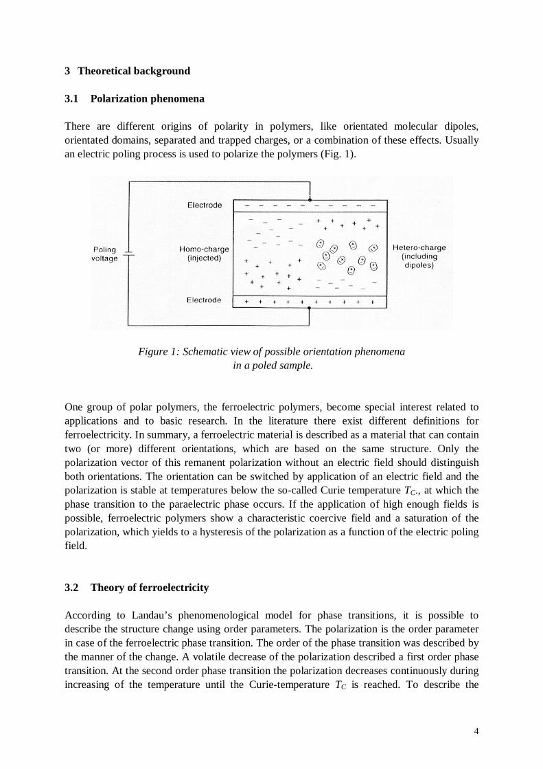
There are different origins of polarity in polymers, like orientated molecular dipoles,orientated domains, separated and trapped charges, or a combination of these effects. Usuallyan electric poling process is used to polarize the polymers (Fig. 1).

Figure 1: Schematic view of possible orientation phenomena in a poled sample.

One group of polar polymers, the ferroelectric polymers, become special interest related toapplications and to basic research. In the literature there exist different definitions forferroelectricity. In summary, a ferroelectric material is described as a material that can containtwo (or more) different orientations, which are based on the same structure. Only thepolarization vector of this remanent polarization without an electric field should distinguishboth orientations. The orientation can be switched by application of an electric field and thepolarization is stable at temperatures below the so-called Curie temperature TC., at which thephase transition to the paraelectric phase occurs. If the application of high enough fields ispossible, ferroelectric polymers show a characteristic coercive field and a saturation of thepolarization, which yields to a hysteresis of the polarization as a function of the electric polingfield.

3.2 Theory of ferroelectricity

According to Landau’s phenomenological model for phase transitions, it is possible todescribe the structure change using order parameters. The polarization is the order parameterin case of the ferroelectric phase transition. The order of the phase transition was described bythe manner of the change. A volatile decrease of the polarization described a first order phasetransition. At the second order phase transition the polarization decreases continuously duringincreasing of the temperature until the Curie-temperature TC is reached. To describe the

5

ferroelectric phase transition the free energy density F (or the Gibbs function G) is expandedin terms of the polarization P as shown in equation (1) ([Devonshire 54], [Smolenskij 84]).

F(T,P) = F0(T) + 1

2α(T)P2 +

1

4γ(T)P4 +

1

6δ(T)P6 (1)

In equation (1) it was assumed that F is symmetrical with respect to P. F0 is the free energydensity of the paraelectric phase. F, α, γ and δ are functions of temperature T.The consideration was limited by the expansion up to the sixth term of the order parameter,furthermore mechanical deformations are negligible and to simplify only one-dimensionalferroelectrics are described.The free energy density has a minimum in thermodynamic equilibrium, therefore theequations (2) must be fulfilled.

P

F

∂∂

= 0,2

2

P

F

∂∂

> 0 (2)

Differentiating F with respect to P yields

P

F

∂∂

= α(T)P + γ(T)P3 + δ(T)P5,2

2

P

F

∂∂

= α(T) + 3γ(T)P2 + 5δ(T)P4. (3)

From (2) and (3) it follows for the non-polar case (P = 0) that α must be greater than zero. Tosolve the condition (2) also in the polar case (P ≠ 0), α must change its sign at the transitiontemperature TC. This can be mathematically achieved using the assumption (4) (Devonshireapproximation).

α = α0(T−TC) (4)

Therefore equation (5) follows to describe F as a function of P.

F(P) = F0 + 1

2α0(T−TC)P2 +

1

4γP4 +

1

6δP6 (5)

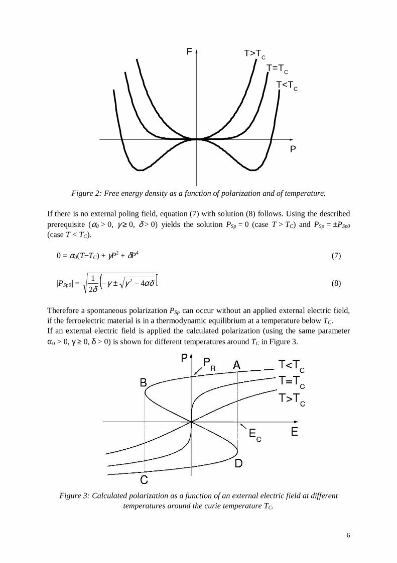
Different possibilities for first-order or second-order phase transitions according to theparameter α, γ, δ, T and TC follow from equation (5), which are discussed in the literature(e.g. [Furukawa 89]).The free energy density F as a function of polarization P for the second-order phase transition(α0 > 0, γ ≥ 0 and δ > 0) is shown in Figure 2 for different values of the parameter α.According to equation (4) the different cases α < 0, α = 0 and α > 0, respectively, aredescribing the behavior below, at and above the Curie temperature TC.Differentiating F with respect to P yields the dependence of the polarization as a function ofthe electric field (6).

E = α0(T−TC)P + γP3 + δP5 (6)

6

T=TC

F

P

T<TC

T>TC

Figure 2: Free energy density as a function of polarization and of temperature.

If there is no external poling field, equation (7) with solution (8) follows. Using the describedprerequisite (α0 > 0, γ ≥ 0, δ > 0) yields the solution PSp = 0 (case T > TC) and PSp = ±PSp0

(case T < TC).

0 = α0(T−TC) + γP2 + δP4 (7)

|PSp0| = ( )αδγγδ

42

1 2 −±− (8)

Therefore a spontaneous polarization PSp can occur without an applied external electric field,if the ferroelectric material is in a thermodynamic equilibrium at a temperature below TC.If an external electric field is applied the calculated polarization (using the same parameterα0 > 0, γ ≥ 0, δ > 0) is shown for different temperatures around TC in Figure 3.

Figure 3: Calculated polarization as a function of an external electric field at differenttemperatures around the curie temperature TC.

7

In the case T < TC the polarization dependence corresponds to an unstable condition betweenthe points B and D. Therefore during poling of an idealized ferroelectric material withincreasing absolute values of the electric field a jump occurs, i.e. a discontinuity place, in thepolarization at positive and negative electric field, respectively. These are symbolized inFigure 3 by dotted lines between A and D as well as B and C. Such a behavior results in ahysteresis of the polarization as a function of the electric field, with significant values for theremanent polarization PR and the coercive field EC.Therefore a ferroelectric polymer shows a P(E)-hysteresis under special conditions, i.e. duringapplication of a high enough poling field at a temperature below TC. However, it has beenshown ([Lines 77]), that no ferroelectric properties can be concluded from a measuredhysteresis during poling of a material. The hysteresis behavior is a necessary but not sufficientcondition.

3.3 Electric poling of ferroelectric polymers

As explained before, different processes, e.g. dipole orientation, orientation of domains,movement and trapping of charges, aging effects, etc. can occur during electrical poling. Toinvestigate and to separate these effects different procedures have been developed for theelectrical poling of polymers or other polar materials. Special procedures also exist for polingof ferroelectric polymers, based on the build up of a remanent polarization after a firstapplication of an electric field.Usually to characterize the orientation phenomena the poling current or the charge build upare measured during the electrical poling process. Here we focus on the description of thepoling current, according to the experimental setup in the lab experiment.The poling current can contain different origins (eq. (9)), e.g. a possible polarization build upIp, a capacitive charging Ic as well as a current based on the conductivity Icon of the sample. Ais the sample area, C the sample capacitance, Vp the poling voltage and R the resistance.

I(t) = Ip(t) + Ic(t) + Icon(t) = dt

AdP+

dt

CdVP +R

VP (9)

If we neglect aging effects, it is possible to separate the contributions to the poling currentusing special measurement procedures. Useful also for the interpretation of microscopicsample properties are poling procedures with constant and (e.g. sinusoidally) varying electricfields.

Poling with constant electric fields

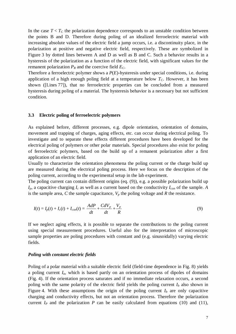
Poling of a polar material with a suitable electric field (field-time dependence in Fig. 8) yieldsa poling current Ia, which is based partly on an orientation process of dipoles of domains(Fig. 4). If the orientation process saturates and if no immediate relaxation occurs, a secondpoling with the same polarity of the electric field yields the poling current Ib also shown inFigure 4. With these assumptions the origin of the poling current Ib are only capacitivecharging and conductivity effects, but not an orientation process. Therefore the polarizationcurrent IP and the polarization P can be easily calculated from equations (10) and (11),

8

respectively. For the calculation (11) it was assumed that the sample was previously poledwith opposite field polarity.

IP(t) = Ia(t) − Ib(t) (10)

P = �

dttIA P )(

2

1(11)

Figure 4: Theoretical currents during poling of polar materials with constant electric fields ofthe same polarity (assuming the saturation of the orientation process).

The advantage of such switching experiments is that the switching time of the orientationprocess can be determined, if the time resolution of the experimental equipment is highenough.

Poling with varying electric fields

Usually poling with varying electric fields is performed using a sinusoidal or triangular time-shape of the electric field. Performing of orientation processes in the polymer using differentcombinations of poling cycles with positive or negative polarities (e.g. Figures 10 and 11)gives the possibility to analyze hysteresis phenomena in the polymer.For poling with varying fields the same physical consideration can be carried out to separatethe contributions in the poling current.

Checkpoint: Discuss the proposed separation of the different current contributions to thepoling current during poling with bipolar electric fields according to the reference[Dickens 92].

9

4 Experiment

4.1 Polymer samples

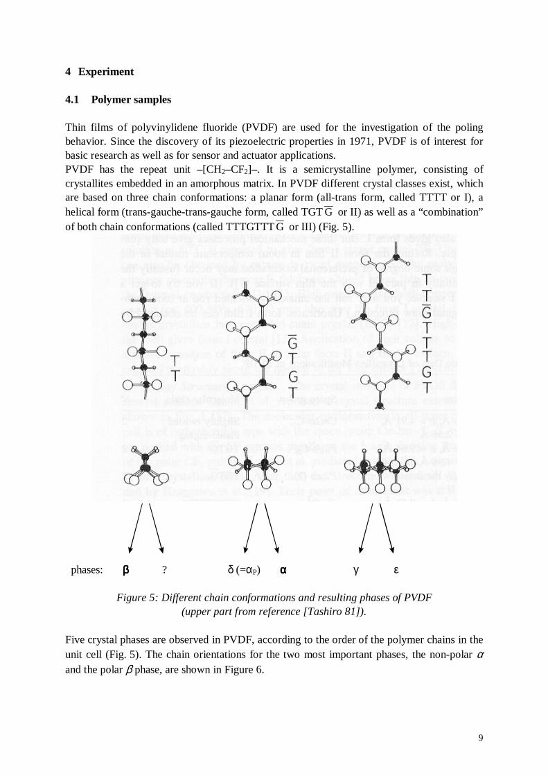
Thin films of polyvinylidene fluoride (PVDF) are used for the investigation of the polingbehavior. Since the discovery of its piezoelectric properties in 1971, PVDF is of interest forbasic research as well as for sensor and actuator applications.PVDF has the repeat unit –[CH2–CF2]–. It is a semicrystalline polymer, consisting ofcrystallites embedded in an amorphous matrix. In PVDF different crystal classes exist, whichare based on three chain conformations: a planar form (all-trans form, called TTTT or I), ahelical form (trans-gauche-trans-gauche form, called TGT G or II) as well as a “combination”of both chain conformations (called TTTGTTT G or III) (Fig. 5).

phases: ββββ ? δ (=αP) αααα γ ε

Figure 5: Different chain conformations and resulting phases of PVDF(upper part from reference [Tashiro 81]).

Five crystal phases are observed in PVDF, according to the order of the polymer chains in theunit cell (Fig. 5). The chain orientations for the two most important phases, the non-polar αand the polar β phase, are shown in Figure 6.

10

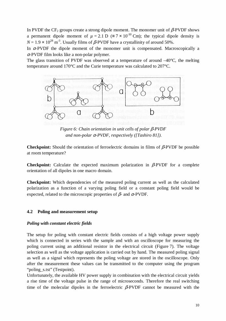
In PVDF the CF2 groups create a strong dipole moment. The monomer unit of β-PVDF showsa permanent dipole moment of µ = 2.1 D (≡ 7 × 10-30 Cm); the typical dipole density isN = 1.9 × 1028 m-3. Usually films of β-PVDF have a crystallinity of around 50%.In α-PVDF the dipole moment of the monomer unit is compensated. Macroscopically aα-PVDF film looks like a non-polar polymer.The glass transition of PVDF was observed at a temperature of around –40°C, the meltingtemperature around 170°C and the Curie temperature was calculated to 207°C.

Figure 6: Chain orientation in unit cells of polar β-PVDF and non-polar α-PVDF, respectively ([Tashiro 81] ).

Checkpoint: Should the orientation of ferroelectric domains in films of β-PVDF be possibleat room temperature?

Checkpoint: Calculate the expected maximum polarization in β-PVDF for a completeorientation of all dipoles in one macro domain.

Checkpoint: Which dependencies of the measured poling current as well as the calculatedpolarization as a function of a varying poling field or a constant poling field would beexpected, related to the microscopic properties of β- and α-PVDF.

4.2 Poling and measurement setup

Poling with constant electric fields

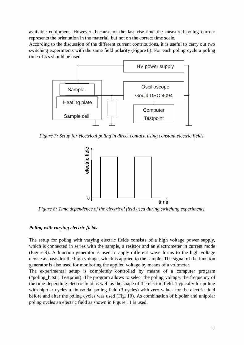
The setup for poling with constant electric fields consists of a high voltage power supplywhich is connected in series with the sample and with an oscilloscope for measuring thepoling current using an additional resistor in the electrical circuit (Figure 7). The voltageselection as well as the voltage application is carried out by hand. The measured poling signalas well as a signal which represents the poling voltage are stored in the oscilloscope. Onlyafter the measurement these values can be transmitted to the computer using the program“poling_s.tst” (Testpoint).Unfortunately, the available HV power supply in combination with the electrical circuit yieldsa rise time of the voltage pulse in the range of microseconds. Therefore the real switchingtime of the molecular dipoles in the ferroelectric β-PVDF cannot be measured with the

11

available equipment. However, because of the fast rise-time the measured poling currentrepresents the orientation in the material, but not on the correct time scale.According to the discussion of the different current contributions, it is useful to carry out twoswitching experiments with the same field polarity (Figure 8). For each poling cycle a polingtime of 5 s should be used.

HV power supply

Oscilloscope

Gould DSO 4094Sample

Heating plate

Computer

TestpointSample cell

Figure 7: Setup for electrical poling in direct contact, using constant electric fields.

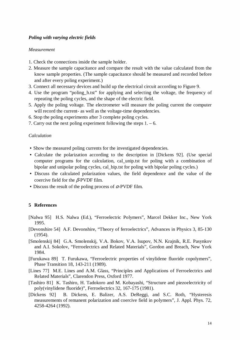
Figure 8: Time dependence of the electrical field used during switching experiments.

Poling with varying electric fields

The setup for poling with varying electric fields consists of a high voltage power supply,which is connected in series with the sample, a resistor and an electrometer in current mode(Figure 9). A function generator is used to apply different wave forms to the high voltagedevice as basis for the high voltage, which is applied to the sample. The signal of the functiongenerator is also used for monitoring the applied voltage by means of a voltmeter.The experimental setup is completely controlled by means of a computer program(“poling_h.tst” , Testpoint). The program allows to select the poling voltage, the frequency ofthe time-depending electric field as well as the shape of the electric field. Typically for polingwith bipolar cycles a sinusoidal poling field (3 cycles) with zero values for the electric fieldbefore and after the poling cycles was used (Fig. 10). As combination of bipolar and unipolarpoling cycles an electric field as shown in Figure 11 is used.

12

ElectrometerHP 3458A

Sample

Heating plate

ComputerTestpoint

FUG HCB 7-6500

Function generatorHP 33120A

MultimeterHP 34401A

RV

Sample cell

Figure 9: Setup for electrical poling in direct contact, using varying electric fields

Figure 10: Time dependence of the electrical field used during poling with bipolar poling cycles.

Figure 11: Time dependence of the electrical field used during poling with a combination of bipolar and unipolar poling cycles.

13

4.3 Running the Experiment

The samples are inserted in different sample holders; the sample surfaces are connected to aninsulated BNC connector. These connections have to be prepared at least one day before thepoling experiments, allowing the connecting glue to set.

Poling with constant electric fields

Measurement

1. Check the connections inside the sample holder.2. Measure the sample capacitance and compare the result with the value calculated from the

know sample properties. (The sample capacitance should be measured and recorded beforeand after every poling experiment.)

3. Connect all necessary devices and build up the electrical circuit according to Figure 7.After checking the electrical circuit, disconnect the sample holder from the HV powersupply.

4. Select the first poling voltage using the potentiometer of the HV power supply.5. Check the applied voltage using a measurement of the “1/1000” output of the HV power

supply with the oscilloscope. Optimize the voltage selection.6. Connect the sample to the HV power supply.7. Set the correct trigger level and measurement level at the oscilloscope.8. Apply the poling voltage; the oscilloscope will measure the current- as well as the voltage-

time dependence.9. Store the measured dependencies at the oscilloscope.10. Stop the poling experiment after 5 seconds.11. Use the program “poling_s.tst” to read out the measured data from the oscilloscope.12. Carry out more than one switching experiments for each sample at each voltage.13. Carry out the next poling experiment following the steps 1. – 12.

Calculation

• Compare the measured currents during switching experiment for each sample / dependence. • Calculate and set the new time basis. • Calculate the polarization according to equation (11). (Use the second switching process, so

that the assumptions of (11) are fulfilled. • Discuss the calculated polarization values for the β-PVDF film and the result of the poling

process on the α-PVDF sample.

14

Poling with varying electric fields

Measurement

1. Check the connections inside the sample holder.2. Measure the sample capacitance and compare the result with the value calculated from the

know sample properties. (The sample capacitance should be measured and recorded beforeand after every poling experiment.)

3. Connect all necessary devices and build up the electrical circuit according to Figure 9.4. Use the program “poling_h.tst” for applying and selecting the voltage, the frequency of

repeating the poling cycles, and the shape of the electric field.5. Apply the poling voltage. The electrometer will measure the poling current the computer

will record the current- as well as the voltage-time dependencies.6. Stop the poling experiments after 3 complete poling cycles.7. Carry out the next poling experiment following the steps 1. – 6.

Calculation

• Show the measured poling currents for the investigated dependencies. • Calculate the polarization according to the description in [Dickens 92]. (Use special

computer programs for the calculation, cal_unip.tst for poling with a combination ofbipolar and unipolar poling cycles, cal_bip.tst for poling with bipolar poling cycles.)

• Discuss the calculated polarization values, the field dependence and the value of thecoercive field for the β-PVDF film.

• Discuss the result of the poling process of α-PVDF film.

5 References

[Nalwa 95] H.S. Nalwa (Ed.), “Ferroelectric Polymers”, Marcel Dekker Inc., New York1995.

[Devonshire 54] A.F. Devonshire, “Theory of ferroelectrics”, Advances in Physics 3, 85-130(1954).

[Smolenskij 84] G.A. Smolenskij, V.A. Bokov, V.A. Isupov, N.N. Krajnik, R.E. Pasynkovand A.I. Sokolov, “Ferroelectrics and Related Materials”, Gordon and Breach, New York1984.

[Furukawa 89] T. Furukawa, “Ferroelectric properties of vinylidene fluoride copolymers”,Phase Transition 18, 143-211 (1989).

[Lines 77] M.E. Lines and A.M. Glass, “Principles and Applications of Ferroelectrics andRelated Materials”, Clarendon Press, Oxford 1977.

[Tashiro 81] K. Tashiro, H. Tadokoro and M. Kobayashi, “Structure and piezoelectricity ofpoly(vinylidene fluoride)”, Ferroelectrics 32, 167-175 (1981).

[Dickens 92] B. Dickens, E. Balizer, A.S. DeReggi, and S.C. Roth, “Hysteresismeasurements of remanent polarization and coercive field in polymers”, J. Appl. Phys. 72,4258-4264 (1992).