Chapter 2

Scattering forces

“Untersuchungen ber die Druckkrafte des Lichtes” by Peter Lebedew (Lebe-dew, 1901)

“Radiation in the solar system” by J. H. Poynting (Poynting, 1904a)

“Radiation in the solar system: its effect on temperature and its pressure onsmall bodies” by J. H. Poynting (Poynting, 1904b)

“Contributions of John Henry Poynting to the understanding of radiationpressure” by R. Loudon and C. Baxter (Loudon & Baxter, 2012)

“Radiation forces on small particles in the solar system” by Joseph A. Burnsand Philippe L. Lamy and Steven Soter (Burns & al., 1979)

2.1 Photons and particle

Scattering event between ‘photon’ and ‘particle’ (or ‘atom’).

Energy conservation, elastic scattering: |k| = |k0|. (Exercise: recoil shift.)

Momentum conservation, momentum transfer:

p

0A � pA = ~(k� k

0) (2.1)

Average over many scattering events, collimated beam, isotropic re-emission

k� k

0= k (2.2)

Typical expression (Cohen-Tannoudji, laser cooling).

radiation pressure force: F

rad

= ~kpe�e (2.3)

2

with scattering rate pe�e. Background: two-level atom with states |gi and|ei. Population/probability pe of excited state. Decay rate �e, lifetime ⌧e =

1/�e of excited state (like radioactive decay).

Order of magnitude: ⇠ 10

5

m/s

2, huge compared to gravity. Typical number⌧e ⇠ 50 ns, mass M = 100 amu, population pe ⇠ 1/2, visible light wave-length 500 nm.

Link to classical electrodynamics: scattering rate and (total) cross section

pe�e =|S(r)|~! �

tot

(2.4)

with Poynting vector S(r) (energy / area / time). Re-interpret as numberof photons / area / time by dividing by ~!. Cross-section �

tot

is an effec-tive area. Simple model of harmonically bound charge (electrodynamicslecture): �

tot

⇠ �

2 possible on resonance.

Re-write radiation pressure (2.3) with the Poynting vector for collimatedbeam (k and S are parallel):

F

rad

= k

|S(r)|!

�

tot

=

S(r)

c

�

tot

(2.5)

using the free space dispersion relation ! = c|k|. Hence interpret S(r)/c asa pressure (force/area) associated with the light beam.

Key concept from momentum balance Eq.(2.2): recoil momentum ±~k atabsorption and emission events.

2.2 Photons reflected at a surface

Incident beam: angle ✓ with normal, reflected beam: angle ✓

0 (need eventu-ally an average for a diffusely reflecting surface).

Balance for normal component of momentum, absorption and re-emission

P

abs

=

~!c

cos ✓, P

em

=

~!0

c

cos ✓

0 (2.6)

Positive if a ‘pressure force’ (the light pushes the mirror).

3

Translated into pressure (need projected area, hence the cos ✓) with incidentPoynting vector S = |S)

p =

S

c

cos ✓

�cos ✓ + cos ✓

0� (2.7)

Observe that both absorption and re-emission give a ‘recoil push’ in the samedirection. This is different from the atom (particle) where the emission wasisotropic.

Numerical value for sunlight, integrated over the entire spectrum. See prob-lem sheet 1: the spectrum is in good approximation that of a black body. Theresulting Poynting vector at the surface of Earth is known as the

‘solar constant’ S ⇡ 1367

W

m

2

(2.8)

so that the associated pressure (assuming that Earth is a specularly reflectingmirror, cos ✓0 = cos ✓) is in order of magnitude (normal incidence, sun inzenith)

p ⇠ 2S

c

⇠ 10

�5

Pa (2.9)

This is negligible compared to the atmospheric pressure – and high up in theatmosphere where the pressure drops, there is no efficient reflection takingplace.

You estimate in the problem sheet that this radiation pressure is also neg-ligible when it is integrated over the cross section of the Earth – at leastcompared to the gravitational force between Sun and Earth. We shall seethat radiation pressure becomes significant for smaller objects in the solarsystem.

Exercise: estimation for a small mirror and a cavity. Go back to photonpicture, introduce ‘round-trip time’ ⌧ = 2L/c with cavity length L. Assumethat the mirror is moving in a harmonic potential with spring constant M⌦

2

and estimate the displacement due to the radiation pressure for one photon,in units of the light wavelength.

4

Chapter 3

Continuous media

“The enigma of optical momentum in a medium” by Stephen M. Barnett andRodney Loudon (Barnett & Loudon, 2010)

3.1 Radiation force on a liquid surface

Experiment performed in 1973 by Ashkin & Dziedzic (1973). Theory workedout by Lai & Young (1976). Our discussion follows closely Brevik (1979).

3.1.1 Experimental setting

For the typical parameters, see below in the text. A pulsed laser beam (wave-length 530 nm), focused near the water surface, is incident from above. Oneobserves that the water ‘bulges’ upward as the beam enters. This createsa convex lens that focuses the beam: one observes that the focal length isfirst very large, goes through a minimum O(200µm) and the focusing dis-appears again. The typical time scale is O(100 � 500 ns), much longer thanthe duration of the laser pulse (⇠ 60 ns).

5

168 1. Brevik, Experiments in phenomenological electrodynamics and the electromagnetic energy-momentum tensor

Fig. 6. Shape of beam focused on the free liquid surface.

that a local hydrodynamical description of the liquid should be appropriate. For we recall fromthe previous subsection that the mean time between two molecular collisions in the liquid is onlyof the order of a picosecond, which is much less than the experimental time scale. We can thereforeintroduce the concept of a local hydrodynamical pressure p. Moreover, we observe that thedimensions are such that the time required for the beam to traverse the liquid is only about 0.01 ns.This enables us to make the assumption that the electromagnetic forces start to act simultaneouslythroughout the liquid. The motion of the free surface is determined by the electromagnetic surfaceforce, the electrostriction force, gravity, and surface tension.Assuming that the beam is switched on at the instant t = 0, we obtain the following picture

for the distribution of forces that govern the motion of the liquid. In those interior regions of theliquid where the field is inhomogenous, electrostrictive compressive forces immediately arise. Theproduced elastic deformations propagate inwards at the speed of sound u. In addition, at the freesurface there act electrostriction forces tending to press the surface downwards. The magnitudeof this force, per unit surface area, is

—~s0E2pdn2/dp = —*C

0E2(n2 — 1) (n2 + 2), (4.30)

where the minus sign signifies that the force acts downwards. The electric field E is the rms-valueof the net field at the free surface, thus equal to the field in the transmitted wave when we ignorethe influence from reflections at the lower boundary of the liquid.Apart from the surface force density (4.30), the free surface is subject also to the Abraham—

Minkowski surface force density acting upwards:

a~’= a~’= ~C0E2(n2— 1). (4.31)

This result is found by integrating the z-component of the force density (1.3) over the boundarylayer of the free surface. In the Abraham case, the additive Abraham term appearing in (1.6)describes avolume effect which obviously gives no contribution after integration over the boundarylayer. The Abraham and Minkowski surface force expressions are thus identical. It is necessaryto stress this point, because statements to the contrary have recently appeared [45].Just after the onset of the pulse the free surface is subject to the combined effect of the forces

(4.30) and (4.31). Note that the negative force (4.30) is stronger than the positive force (4.31), sothat the net electromagnetic force in reality acts downwards to begin with. (Recall the analogous

3.1.2 Short times: sound waves

Hydrodynamic description for the first few ns of the pulse. Brevik focuseson the electrostriction force: this is a volume force with density

f

es

= r�, � =

1

2

E

2

%

@"

@%

(3.1)

where % is the mass density and " the dielectric function of the liquid. Inthe standard arguments for electrostriction, the derivative @"/@% is takenat constant temperature. Due to the short time scales (a few ns), one mayrather take the adiabatic regime (constant entropy), considering that theexchange of heat is too slow to enforce a constant temperature.

The force density on the liquid gives the equation of motion for the velocityfield (the Euler equation)

%

@v

@t

= �rp+r� (3.2)

where p is the hydrodynamic pressure. We neglect viscosity here. FromEq.(3.2), we see that the vorticity r ⇥ v can be taken as zero at all times.Hence, we can express the velocity in terms of a velocity potential �

v = r� (3.3)

and get from the Euler equation, up to a spatially constant reference value(for the pressure):

%

@�

@t

= �p+ � (3.4)

The equation of continuity is

0 =

@%

@t

+r · (%v) = d%

dt

+ %r · v (3.5)

6

where d/dt = @/@t+v ·r is the co-moving (or substantial) derivative.

We take the substantial derivative of the Euler Eq.(3.4) and neglect termsquadratic in the velocity (sound waves of small amplitude). This gives onthe left-hand side

d

dt

%

@�

@t

⇡ %

@

2

�

@

2

t

(3.6)

On the right-hand side, we express the pressure change in terms of thechange in density, assuming that at each instant, we have an equation ofstate

�dp

dt

+

d�

dt

= �@p

@%

d%

dt

+

d�

dt

⇡ +u

2

%r · v +

@�

@t

(3.7)

where in the last step, the continuity Eq.(3.5) was used. (We also assumethat the speed of sound u, given by u

2

= @p/@% taken at constant entropy,is a constant.) The divergence r · v becomes a second derivative of thevelocity potential so that we get:

@

2

�

@

2

t

� u

2r2

� =

1

%

@�

@t

(3.8)

This is a wave equation with a source term. The dispersion relation for thesound waves follows from a plane wave ansatz �(r, t) ⇠ exp i(k · r � !t)

as! = u|k| (3.9)

The source term on the right-hand side (rhs) of Eq.(3.8) is the volumeforce density due to electrostriction. The boundary conditions at the wa-ter surface z = h(x, y) is that the velocity there equals the change in height:vz(x, y, h) = @th(x, y). The simplest approximation to calculate the sound inthe bulk of the water is to assume that the water surface remains flat h = 0.This gives vz(x, y, 0) = @z�(x, y, 0) = 0, a so-called von Neumann boundarycondition.

Brevik solves the inhomogeneous wave equation (3.8) with the ‘method ofimages’, using a gaussian beam approximation for the light intensity distri-bution in the liquid. One finds that the pressure at the surface, p(x, y, 0, t) inthe center of the beam rises on a time scale O(w

0

/u) given by the beam waistw

0

and the speed of sound. Typical numbers are w

0

/u ⇠ 2µm/10

3

m/s =

2 ns. Long after this time, sound waves leave into the bulk of the water, andthe pressure equilibrates to compensate for the electrostrictive force density:p = � in Eq.(3.4).

Longer times: surface force and tension

In the experiment of Ashkin & Dziedzic, the laser was pulsed with a timemuch longer than 1ms. What happens at longer times is that the water

7

surface changes. To simplify the calculations, Brevik adopts the model of anideal (no viscosity) and incompressible fluid. The density % is then constant,and the pressure p becomes an independent dynamical variable. In addition,one has to apply boundary conditions for the force density at the surface thattake into account surface tension. For completeness, we also include gravityhere (natural if the pressure rises deep in the water).

For technical details on surface tension, see the lecture by John W. M. Bushfrom MIT (Boston), online athttp://web.mit.edu/1.63/www/Lec-notes/Surfacetension/Lecture2.pdf

The density of forces in the bulk of the water, incompressible and neglectingviscosity, becomes

d

dt

(%v) = %

d

dt

v = �rp+ %g (3.10)

where d/dt = @/@t + v · r is the convective derivative and g = �gez theacceleration vector due to gravity. (We take the z-axis pointing upwards,from water to air.) When linearized for small v, this equation gives dv/dt ⇡@tv.

We represent the velocity field again by a potential, v = r� and get fromthe equation of continuity

0 = @t%+r · (%v) = d%

dt

+ %(r · v) = %(r · v) (3.11)

so that we have the simple Laplace equation r2

� = 0.

When we integrate the force Eq.(3.10) along the z-axis, we get

%@t�(r) = �p(r)� %gz (3.12)

This is value up to just below the surface at z = h(x). We can use thefreedom of choosing the integration constant to define that the pressurep = 0 at the surface.

In the water surface, we have to add the force densities due to the opticalforce and due to surface tension. The optical force per area is given by thedifference in the electromagnetic stress tensors in air (dielectric constant 1)and in water (" = n

2 with n ⇡ 1.33 in the visible range):

Tzz ="

0

2

(n

2 � 1)E

2

(x, h, t) (3.13)

where E

2

(x, h, t) is the light intensity evaluated at the surface. Note thatthis formula is the same for both viewpoints, by Minkowski and Abraham,on the energy-momentum tensor.

8

The surface tension � depends on the curvature of the surface (see the lec-ture by Bush mentioned above):

� = �(

1

R

1

+

1

R

2

) = �(rs · ˆn) (3.14)

where � is the surface tension and R

1,2 are the principal radii of curvature.The curvature is calculated from the unit vector ˆ

n normal to the surface(pointing from the liquid into air) and rs·, the divergence evaluated alongthe surface. (This is natural since the vector field ˆ

n ‘lives’ only on the sur-face.) For clean water (no soap!), a typical value for the surface tension is� ⇡ 0.073 J/m

2.

For a surface described by the height function z = h(x), the normal vectorcan be constructed from the gradient

ˆ

n =

r(z � h(x))

|r(z � h(x))| =ez �rsh

(1 + (rsh)2

)

1/2(3.15)

Expanding this to first order in h, we get for the curvature the expres-sion

rs · ˆn ⇡ �r2

sh (3.16)

so that the surface tension is proportional to the second derivative of theheight function.

Finally, by adding surface tension and the optical surface force to Eq.(3.12),the balance of surface stresses takes the form (recall that p = 0 at the sur-face)

%@t� = �%gh+ �r2

sh+

"

0

2

(n

2 � 1)E

2

(x, h, t) (3.17)

To complete the equations, we have to apply the boundary condition for themotion of the surface: the vertical velocity is equal to the rate of change ofthe height

@th(x) = vz(x, h) = @z�(x, h) (3.18)

This is known as a ‘free surface’. (A ‘fixed surface’ would correspond toh = 0, for example.)

Solving for the surface deformation

The hydrodynamic equations derived so far provide a description for waterwaves, also known as capillary waves. We shall make the small-amplitudeapproximation and continue to work to lowest order in h. This means, forexample, that in the free surface condition (3.18) the velocity potential canbe evaluated at z = 0: �(x, h) ⇡ �(x, 0).

9

To analyze the water wave equation (3.17), we assume a solution in theform of a plane wave exp ik ·x (here, k is a two-dimensional wave vector inthe surface). From the Laplace equation in the bulk for �, we get

0 = r2

�(k, z) = �k

2

�+ @

2

z� (3.19)

This can be solved by exponentials e±kz with k = |k|. The physical solutionthat remains finite ‘deep inside the water’ is �(k, z) = �(k) e

kz. Evaluatedat the (approximate) surface z = 0, this gives us the derivative @z� = k�.The condition for the free surface therefore yields � = (1/k)@th so that thewave equation becomes

%@

2

t h+ %gkh+ �k

3

h = kI(k, h, t) ⇡ kI(k, 0, t) (3.20)

where I =

1

2

"

0

(n

2 � 1)E

2 is the optical surface stress. We again used thesmall-amplitude approximation. This is a wave equation with a ‘source term’provided by the optical stress. The left-hand side (lhs) of Eq.(3.20) gives thedispersion relation of the capillary waves: we assume a time dependenceh ⇠ e

�i!t and get

!

2

= gk +

�

%

k

3

= gk(1 + (k�)

2

), �

2

=

�

%g

(3.21)

The length � is called the ‘capillary length’, its value for water and gravityat the surface of earth is � ⇡ 2.7mm. For wavelength much larger than this,surface tension can be neglected, and we find the dispersion relation

k� ⌧ 1 : ! ⇡p

gk, vg ⇡r

g

4k

(3.22)

Exercise. Get typical numbers for the group velocity vg: waves on the beach,very-long wavelength waves on the ocean (note that the penetration depthinto deep water is O(1/k)).

The laser beam that excites surface waves in the experiment has a typicalwidth w

0

of a few microns. In additional, the spatial profile is often a gaus-sian. Adopting the convention that w

0

gives the beam radius where theintensity has fallen by a factor 1/e2, we get for the spatial Fourier transformthe gaussian

I(k, 0, t) = I(t) e

�k2w20/8 (3.23)

where I(t) is proportional to the power of the laser beam and carries thetime-dependence of the laser pulse. With this form, the wave equation tosolve takes the form of a driven oscillator

@

2

t h+ ⌦

2

kh = I(t)k e

�k2w20/8 (3.24)

where ⌦k is the capillary wave dispersion relation (3.21).

10

With a specific model for the pulse shape, Brevik works out the solution toEq.(3.24). The observable that he finally calculates is related to the curva-ture of the water bulge: indeed, as the water is pulled upwards, its curvedsurface acts like a collecting lens that focuses the laser beam. Adopting theapproximation of a spherical lens, geometrical optics yields the inverse focallength

1

f

=

n� 1

n

1

R

⇡ �n� 1

n

r2

sh (3.25)

where R is the radius of curvature and n the index of water relative to air.From the Fourier expansion of h, we get on the beam axis

�r2

sh(0, t) =

Zd

2

k k

2

h(k, t) (3.26)

The result is shown here:I. Brevik, Experiments in phenomenological electrodynamics and the electromagnetic energy-momentum tensor 173

104(m~)

100 200 300 400 500 600 700

Fig. 7. Time development of the inverse focal length 1/f Full line gives the theoretical result calculated from (4.43) with the effectivebeam radius w

0 = 4.5 jnn. Broken line gives the experimental result of Ashkin and Dziedzic [8] displaced by 60 ns to the left.

whereafter it falls relatively slowly. At t ~ 1000 ns the height will have decreased to one half of itsmaximum value.It is worthwhile to summarize the points where the above calculation differs from the pioneering

calculation of Lai and Young:(i) For reasons given above, the form (4.38) for T(t) implies that we have displaced Ashkin and

Dziedzic’s curves by 60 ns to the left.(ii) A correction factor 4(n + ~

2 appears in the main result (4.43) because of the fact that Ein (4.34) means the net tangential field at the surface. The result of Lai and Young corresponds toputting E in (4.34) equal to the field in the incident beam.(iii) Whereas the expression for E2(R) was above taken to be the Gaussian (4.39), the corres-

ponding expression E2(R)Ly in Lai and Young’s theory can be written as

4 p(i) k 3/2E2(R)Ly = (n + 1)2 21rE

0c Idk k J0(kR) exp[—(~~_)] (4.44)

(we have inserted an extra factor 4(n + 1)- 2 in front to make the expression directly comparableto (4.39)). Here k0 is a frequency cut-off parameter that was chosen equal to 0.5 pm 1, i.e. equalto the inverse value of the beam radius given by Ashkin and Dziedzic. The reason for the choice(4.44) was to make the integral in (4.43) amenable to analytic evaluation. *Finally, the following point should be noted. Above we encountered difficulties in reconciling

theory with the Ashkin—Dziedzic result w0 = 2.1 pm for the beam. It is therefore at first somewhatsurprising that Lai and Young obtained reasonable agreement with observation using the Ashkin—Dziedzic input data in an apparently straightforward way. The explanation for this agreementseems, however, to be the following: Theirchoice 0.5 pm~’for the value of the cut-offparameter k0implicitly determines the beam radius to be actually greater than 2 pm. To show this, we calculatethe ratio of the expression (4.44) to the square of the field at the symmetry axis R = 0 (i.e. therelative intensity):

E2(R)Ly — 3 ~ dk kJ

0(kR) exp [—(k/k0)312] 445E2(0)Ly — 2k~f(4/3) . ( . )

~It ought to be mentioned that the exponent 10/3 in the denominator in the last term in the parenthesis in Lai and Young’s eq. (15)should be replaced by 5/3.

The typical focal length (maximum of the curve) is of the order of (1/4)10�4

m =

25µm. It is reached after a time O(300 ns). If we estimate the second deriva-tive in Eq.(3.25) by a factor 1/w2

0

, we get an elevation of the surface of theorder of maxh ⇠ w

2

0

/f ⇠ 0.1 � 1µm, depending on the waist w0

and thenumerical factor involving the index n. This is relatively small and difficultto detect directly. But it roughly validates our assumption that the height his ‘small’ compared to the spot size w

0

. The period of capillary waves withk = 2/w

0

is of the order of 150 ns which is roughly the time scale for thebuild-up in the figure above.

These numbers correspond to an experiment performed with a beam ofpower 3 kW (quite high) and waist w

0

= 2.1µm. For a quantitative eval-uation, one has to take into account that a part is reflected from the watersurface: one needs the field intensity right at the interface which gives an-other factor depending on the index n.

Brevik compares in detail theory and experiment: the maximum of the in-verse focal length is displaced in time with respect to the experimental work– this may be related to the ‘timing’ of the measurement and the uncertaintyin determining the ‘start’ of the pulse. The value for 1/f comes out a factor

11

O(10) too large – this can be improved if a larger value for the beam waistw

0

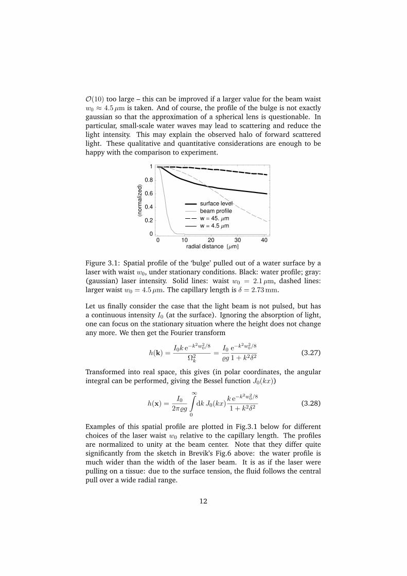
⇡ 4.5µm is taken. And of course, the profile of the bulge is not exactlygaussian so that the approximation of a spherical lens is questionable. Inparticular, small-scale water waves may lead to scattering and reduce thelight intensity. This may explain the observed halo of forward scatteredlight. These qualitative and quantitative considerations are enough to behappy with the comparison to experiment.

0 10 20 30 40radial distance !Μm"

0

0.2

0.4

0.6

0.8

1

#no

rma

lize

d$

surface level

beam profile

w " 45. Μm

w " 4.5 Μm

Figure 3.1: Spatial profile of the ‘bulge’ pulled out of a water surface by alaser with waist w

0

, under stationary conditions. Black: water profile; gray:(gaussian) laser intensity. Solid lines: waist w

0

= 2.1µm, dashed lines:larger waist w

0

= 4.5µm. The capillary length is � = 2.73mm.

Let us finally consider the case that the light beam is not pulsed, but hasa continuous intensity I

0

(at the surface). Ignoring the absorption of light,one can focus on the stationary situation where the height does not changeany more. We then get the Fourier transform

h(k) =

I

0

k e

�k2w20/8

⌦

2

k

=

I

0

%g

e

�k2w20/8

1 + k

2

�

2

(3.27)

Transformed into real space, this gives (in polar coordinates, the angularintegral can be performed, giving the Bessel function J

0

(kx))

h(x) =

I

0

2⇡%g

1Z

0

dk J

0

(kx)

k e

�k2w20/8

1 + k

2

�

2

(3.28)

Examples of this spatial profile are plotted in Fig.3.1 below for differentchoices of the laser waist w

0

relative to the capillary length. The profilesare normalized to unity at the beam center. Note that they differ quitesignificantly from the sketch in Brevik’s Fig.6 above: the water profile ismuch wider than the width of the laser beam. It is as if the laser werepulling on a tissue: due to the surface tension, the fluid follows the centralpull over a wide radial range.

12

Bibliography

A. Ashkin & J. Dziedzic (1973). Radiation Pressure on a Free Liquid Surface,Phys. Rev. Lett. 30 (4), 139–42.

S. M. Barnett & R. Loudon (2010). The enigma of optical momentum in amedium, Phil. Trans. R. Soc. (London) A 368 (1914), 927–39.

I. Brevik (1979). Experiments in phenomenological electrodynamics and theelectromagnetic energy-momentum tensor, Phys. Rep. 52 (3), 133–201.

J. A. Burns, P. L. Lamy & S. Soter (1979). Radiation forces on small particlesin the solar system, Icarus 40 (1), 1–48.

H.-M. Lai & K. Young (1976). Response of a liquid surface to the passage ofan intense laser pulse, Phys. Rev. A 14 (6), 2329–33.

P. Lebedew (1901). Untersuchungen uber die Druckkrafte des Lichtes, Ann.

Phys. (Berlin) 311 (11), 433–58.

R. Loudon & C. Baxter (2012). Contributions of John Henry Poynting tothe understanding of radiation pressure, Proc. Roy. Soc. (London) A 468(2143), 1825–38.

J. H. Poynting (1904a). Radiation in the solar system, Nature 70, 512—15.

J. H. Poynting (1904b). Radiation in the solar system: its effect on tempera-ture and its pressure on small bodies, Phil. Trans. R. Soc. (London) A 202,525–552.

13