phase synchr - uni-potsdam.de
TRANSCRIPT
PHASE SYNCHRONIZATIONOF REGULAR AND CHAOTIC
SELF-SUSTAINED OSCILLATORS
ARKADY S. PIKOVSKY and MICHAEL G. ROSENBLUM
Department of Physics, Potsdam University, Am Neuen Palais19, PF 601553, D-14415, Potsdam, Germany
Abstract
In this review article we discuss eects of phase synchronization of nonlinear
self-sustained oscillators. Starting with a classical theory of phase locking,
we extend the notion of phase to autonoumous continuous-time chaoticsystems. Using as examples the well-known Lorenz and Rossler oscillators,
we describe the phase synchronization of chaotic oscillators by periodic ex-
ternal force. Both statistical and topological aspects of this phenomenon are
discussed. Then we proceed to more complex cases and discuss phase syn-
chronization in coupled systems, lattices, large globally coupled ensembles,
and of space-time chaos. Finally, we demonstrate how the synchronization
eects can be detected from observations of real data.
1. Introduction
Synchronization, a basic nonlinear phenomenon, discovered at the begin-
ning of the modern age of science by Huygens [27], is widely encountered in
various elds of science, often observed in living nature [25, 24] and nds a
lot of engineering applications [7, 8]. In the classical sense, synchronization
means adjustment of frequencies of self-sustained oscillators due to a weak
interaction [49].
The history of synchronization goes back to the 17th century when
the famous Dutch scientist Christiaan Huygens [27] reported on his ob-
servation of synchronization of two pendulum clocks. Systematic study
of this phenomenon, experimental as well as theoretical, was started by
Edward Appleton [3] and Balthasar van der Pol [70]. They showed that
the frequency of a triode generator can be entrained, or synchronized, by a
188 PIKOVSKY AND ROSENBLUM
weak external signal with slightly dierent frequency. These studies were of
high practical importance because such generators became basic elements
of radio communication systems.
Next impact to the development of the theory of synchronization was
given by the representatives of the Russian school. Andronov and Vitt [2, 1]
further developed methods of van der Pol and generalized his results. The
case of n : m external synchronization was studied by Mandelshtam and
Papaleksi [40]. Mutual synchronization of two weakly nonlinear oscillators
was analytically treated by Mayer [41] and Gaponov [23]; relaxation oscil-
lators were studied by Bremsen and Feinberg [9] and Teodorchik [68]. An
important step was done by Stratonovich [64, 65] who developed a theory
of external synchronization of a weakly nonlinear oscillator in the presence
of random noise.
Development of rigorous mathematical tools of the synchronization the-
ory started with Denjoy works on circle map [19] and with treatment of
forced relaxation oscillators by Cartwright and Littlewood [11, 12]. Recent
development has been highly in uenced by Arnold [4] and by Kuramoto
[34].
In the context of interacting chaotic oscillators, several eects are usu-ally referred to as\synchronization" [49, 47, 35]. Due to a strong interaction
of two (or a large number) of identical chaotic systems, their states can coin-
cide, while the dynamics in time remains chaotic [22, 51]. This eect is called
\complete synchronization" of chaotic oscillators. It can be generalized to
the case of non-identical systems [51, 38, 39], or that of the interacting
subsystems [46, 31]. Another well-studied eect is the \chaosdestroying"
synchronization, when a periodic external force acting on a chaotic system
destroys chaos and a periodic regime appears [36], or, in the case of an
irregular forcing, the driven system follows the behavior of the force [32].
This eect occurs for a relatively strong forcing as well. A characteristic
feature of these phenomena is the existence of a threshold coupling value
depending on the Lyapunov exponents of individual systems [22, 51, 6, 20].
In this article we concentrate on the recently described eect of phasesynchronization of chaotic systems, which generalizes the classical notion
of phase locking. Indeed, for periodic oscillators only the relation between
phases is important, while no restriction on the amplitudes is imposed.
Thus, we dene phase synchronization of chaotic system as an appearance
of a certain relation between the phases of interacting systems or between
the phase of a system and that of an external force, while the amplitudes can
remain chaotic and are, in general, non-correlated. This type of synchroniza-
tion has been observed in experiments with electronic chaotic oscillators [52,
45], plasma discharge [69], and electrochemical oscillators [28].
PHASE SYNCHRONIZATION 189
2. Synchronization of periodic oscillators
2.1. PHASE LOCKING
In this section we remind basic facts on the synchronization of periodic
oscillations (see, e.g., [43]). Stable periodic oscillations are represented by a
stable limit cycle in the phase space. The motion of the phase point along
the cycle can be parametrized by the phase (t), it's dynamics obeys
d
dt= !0; (1)
where !0 = 2=T0, and T0 is the period of the oscillation. It is impor-
tant that starting from any monotonically growing variable on the limit
cycle (so that at one rotation increases by ), one can introduce the
phase satisfying Eq. (1). Indeed, an arbitrary obeys _ = () with a
periodic \instantaneous frequency" ( + ) = (): The change of vari-
ables = !0R
0[ ()]1d gives the correct phase, with the frequency !0
being dened from the condition 2 = !0R 0[()]1d: A similar approach
leads to correct angle-action variables in Hamiltonian mechanics. We have
performed this simple consideration to underline the fact that the notions
of the phase and of the phase synchronization are universally applicable to
any self-sustained periodic behavior independently on the form of the limit
cycle.
From (1) it is evident that the phase corresponds to the zero Lyapunov
exponent, while negative exponents correspond to the amplitude variables.
Note that we do not consider the equations for the amplitudes, as they are
not universal.
When a small external periodic force with frequency is acting on this
periodic oscillator, the amplitude is relatively robust, so that in the rst
approximation one can neglect variations of the amplitude to obtain for the
phase of the oscillator and the phase of the external force the equations
d
dt= !0 + "G(; ) ;
d
dt= ; (2)
where G(; ) is 2-periodic in both arguments and " measures the strength
of the forcing. For a general method of derivation of Eq. (2) see [34]. The
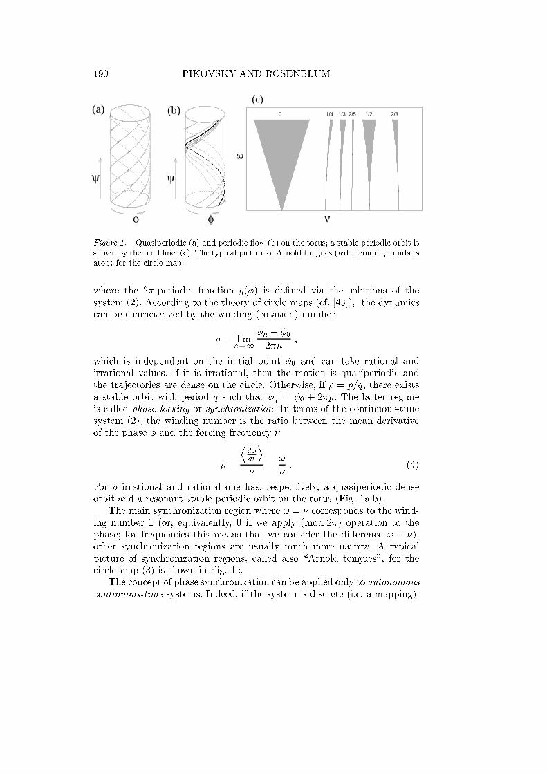
system (2) describes a motion on a 2-dimensional torus that appears from
the limit cycle under periodic perturbation (see Fig. 1a,b). If we pick up
the phase of oscillations stroboscopically at times tn = n2, we get a
circle map
n+1 = n + "g(n) ; (3)
190 PIKOVSKY AND ROSENBLUM
(a)
ψ
φ
(b)
ψ
φ
(c)
νε
0 1/4 1/3 2/5 1/2 2/3
Figure 1. Quasiperiodic (a) and periodic ow (b) on the torus; a stable periodic orbit is
shown by the bold line. (c): The typical picture of Arnold tongues (with winding numbers
atop) for the circle map.
where the 2-periodic function g() is dened via the solutions of the
system (2). According to the theory of circle maps (cf. [43]), the dynamics
can be characterized by the winding (rotation) number
= limn!1
n 0
2n;
which is independent on the initial point 0 and can take rational and
irrational values. If it is irrational, then the motion is quasiperiodic and
the trajectories are dense on the circle. Otherwise, if = p=q, there exists
a stable orbit with period q such that q = 0 + 2p. The latter regime
is called phase locking or synchronization. In terms of the continuous-time
system (2), the winding number is the ratio between the mean derivative
of the phase and the forcing frequency
=
Dd
dt
E
=!
: (4)
For irrational and rational one has, respectively, a quasiperiodic dense
orbit and a resonant stable periodic orbit on the torus (Fig. 1a,b).
The main synchronization region where ! = corresponds to the wind-
ing number 1 (or, equivalently, 0 if we apply (mod 2) operation to the
phase; for frequencies this means that we consider the dierence ! ),
other synchronization regions are usually much more narrow. A typical
picture of synchronization regions, called also \Arnold tongues", for the
circle map (3) is shown in Fig. 1c.
The concept of phase synchronization can be applied only to autonomouscontinuous-time systems. Indeed, if the system is discrete (i.e. a mapping),
PHASE SYNCHRONIZATION 191
its period is an integer, and this integer cannot be adjusted to some other
integer in a continuous way. The same is true for forced continuous-time
oscillations (e.g., for the forced DuÆng oscillator): here the frequency of
oscillations is completely determined by that of the forcing and cannot be
adjusted to some other value. We can formulate this also as follows: in
discrete or forced systems there is no zero Lyapunov exponent, so there is
no corresponding marginally stable variable (the phase) that can be aected
by small external perturbations.
The synchronization condition (4) does not mean that the dierence
between the phase of an oscillator and that of the external force (or
between phases of two oscillators) must be a constant, as is sometimes
assumed (see, e.g. [66]). Indeed, (2) implies, that to enable = const,
the function G should depend not on separate phases but only on their
dierence: G(; ) = G( ). Denoting this phase dierence as ' = we can rewrite Eq. (2) as
d'
dt= !0 + "q(') : (5)
In the synchronous state this equation should have (at least one) stable
point. This happens if the frequency mismatch (detuning) is small enough,
"qmin < !0 < "qmax, and this condition determines the synchronization
(phase-locking, mode-locking) region on the (!; ") plane. Within this region,
the phase dierence remains constant, = Æ, and the value of this constant
depends on the detuning, Æ = q1[( !0)="] (here the stable branch of
the inverse function should be chosen). Generally, the coupling function
G(; ) cannot be reduced to a function of the phase dierence '. Then,
even in a synchronous regime ' is not constant but uctuates, although
these uctuations are bounded. Thus, we can dene phase locking according
to relation
j(t) (t) Æj < const ; (6)
from which the condition of frequency locking h _i = naturally follows.
The latter denition of phase locking will be used in the treatment of chaotic
oscillations below, but even for periodic regimes it has an advantage when
the forced oscillations are not close to the original limit cycle.
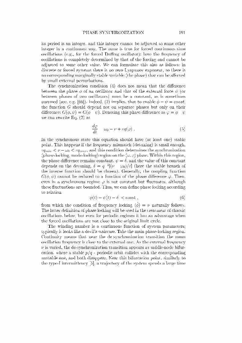
The winding number is a continuous function of system parameters;
typically it looks like a devil's staircase. Take the main phase-locking region.
Continuity means that near the de-synchronization transition the mean
oscillation frequency is close to the external one. As the external frequency
is varied, the de-synchronization transition appears as saddle-node bifur-
cation, where a stable p=q - periodic orbit collides with the corresponding
unstable one, and both disappear. Near this bifurcation point, similarly to
the type-I intermittency [5], a trajectory of the system spends a large time
192 PIKOVSKY AND ROSENBLUM
+
∆
∆
V
V
-
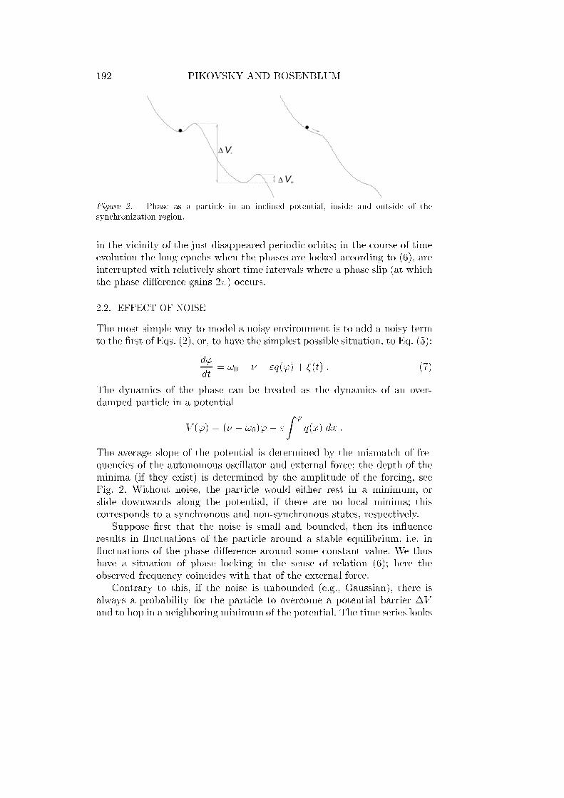
Figure 2. Phase as a particle in an inclined potential, inside and outside of the
synchronization region.
in the vicinity of the just disappeared periodic orbits; in the course of time
evolution the long epochs when the phases are locked according to (6), are
interrupted with relatively short time intervals where a phase slip (at which
the phase dierence gains 2) occurs.
2.2. EFFECT OF NOISE
The most simple way to model a noisy environment is to add a noisy term
to the rst of Eqs. (2), or, to have the simplest possible situation, to Eq. (5):
d'
dt= !0 + "q(') + (t) : (7)
The dynamics of the phase can be treated as the dynamics of an over-
damped particle in a potential
V (') = ( !0)' "
Z'
q(x) dx :
The average slope of the potential is determined by the mismatch of fre-
quencies of the autonomous oscillator and external force; the depth of the
minima (if they exist) is determined by the amplitude of the forcing, see
Fig. 2. Without noise, the particle would either rest in a minimum, or
slide downwards along the potential, if there are no local minima; this
corresponds to a synchronous and non-synchronous states, respectively.
Suppose rst that the noise is small and bounded, then its in uence
results in uctuations of the particle around a stable equilibrium, i.e. in
uctuations of the phase dierence around some constant value. We thus
have a situation of phase locking in the sense of relation (6); here the
observed frequency coincides with that of the external force.
Contrary to this, if the noise is unbounded (e.g., Gaussian), there is
always a probability for the particle to overcome a potential barrier V
and to hop in a neighboring minimum of the potential. The time series looks
PHASE SYNCHRONIZATION 193
0 200 400 600 800 1000time
−30
−20
−10
0
10ϕ/
2πa) b)
c)
d)
−π 0 π
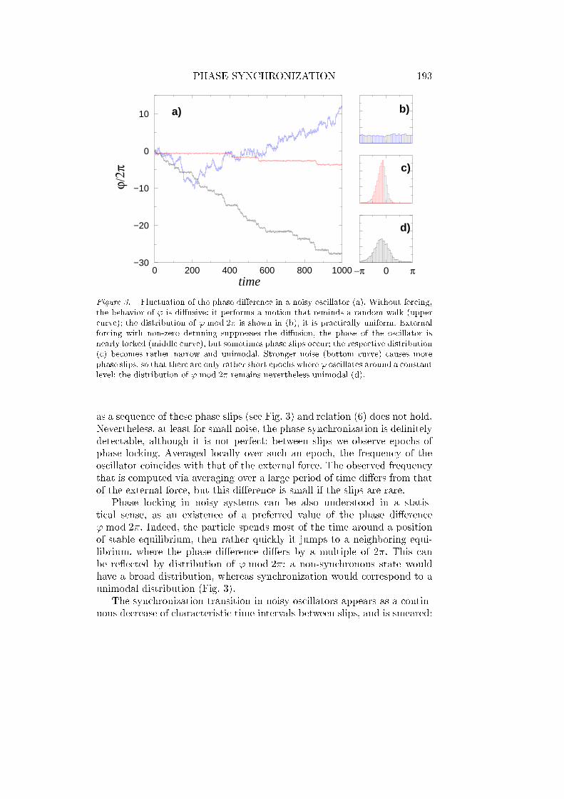
Figure 3. Fluctuation of the phase dierence in a noisy oscillator (a). Without forcing,
the behavior of ' is diusive: it performs a motion that reminds a random walk (upper
curve); the distribution of ' mod 2 is shown in (b), it is practically uniform. External
forcing with non-zero detuning suppresses the diusion, the phase of the oscillator is
nearly locked (middle curve), but sometimes phase slips occur; the respective distribution
(c) becomes rather narrow and unimodal. Stronger noise (bottom curve) causes more
phase slips, so that there are only rather short epochs where ' oscillates around a constant
level; the distribution of ' mod 2 remains nevertheless unimodal (d).
as a sequence of these phase slips (see Fig. 3) and relation (6) does not hold.
Nevertheless, at least for small noise, the phase synchronization is denitely
detectable, although it is not perfect: between slips we observe epochs of
phase locking. Averaged locally over such an epoch, the frequency of the
oscillator coincides with that of the external force. The observed frequency
that is computed via averaging over a large period of time diers from that
of the external force, but this dierence is small if the slips are rare.
Phase locking in noisy systems can be also understood in a statis-
tical sense, as an existence of a preferred value of the phase dierence
' mod 2. Indeed, the particle spends most of the time around a position
of stable equilibrium, then rather quickly it jumps to a neighboring equi-
librium, where the phase dierence diers by a multiple of 2. This can
be re ected by distribution of ' mod 2: a non-synchronous state would
have a broad distribution, whereas synchronization would correspond to a
unimodal distribution (Fig. 3).
The synchronization transition in noisy oscillators appears as a contin-
uous decrease of characteristic time intervals between slips, and is smeared:

194 PIKOVSKY AND ROSENBLUM
−20 −10 0 10 20x
−20.0
−10.0
0.0
10.0
20.0
y
(a)
−15 −10 −5xn
−15
−10
−5
x n+1
6.0
6.1
6.2
6.3
6.4
6.5
retu
rn ti
me
T
(b)
(c)
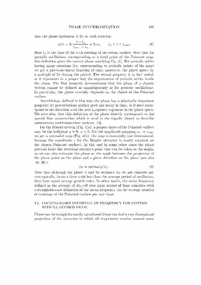
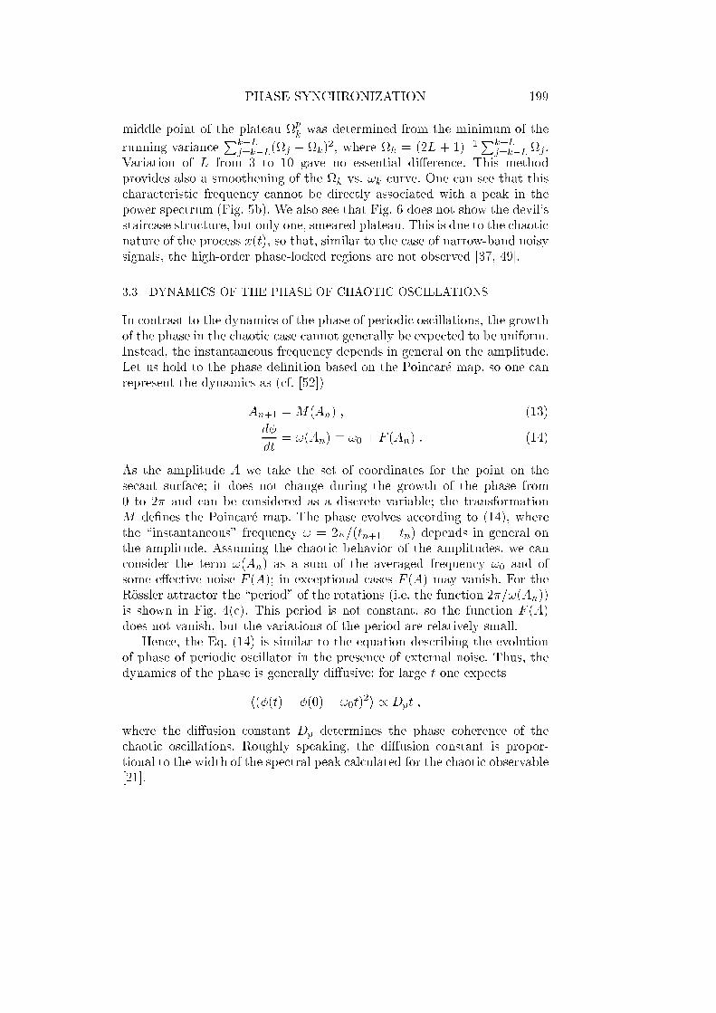
Figure 4. Projection of the phase potrait of the Rossler system (a). The horizontal line
shows the Poincare section that is used for computation of the amplitude mapping (b)
and dependence of the return time (rotation period) on the amplitude (c).
we cannot unambiguously determine the border of this transition.
3. Phase and frequency of a chaotic oscillator
3.1. DEFINITION OF THE PHASE
The rst problem in extending the basic notions from periodic to chaotic
oscillations is to dene properly a phase. There seems to be no unambiguous
and general denition of phase applicable to an arbitrary chaotic process.
Roughly speaking, we want to dene phase as a variable which is related to
the zero Lyapunov exponent of a continuous-time dynamical system with
chaotic behavior. Moreover, we want this phase to correspond to the phase
of periodic oscillations satisfying (1).
To be not too abstract, we illustrate a general approach below on the
well-known Rossler system. A projection of the phase portrait of this au-
tonomous 3-dimensional system of ODEs (see Eqs. (17) below) is shown in
Fig. 4.
Suppose we can dene a Poincare map for our autonomous continuous-
time system. Then, for each piece of a trajectory between two cross-sections
with the Poincare surface we dene the phase just proportional to time, so
PHASE SYNCHRONIZATION 195
that the phase increment is 2 at each rotation:
(t) = 2t tn
tn+1 tn+ 2n; tn t < tn+1: (8)
Here tn is the time of the n-th crossing of the secant surface. Note that for
periodic oscillations corresponding to a xed point of the Poincare map,
this denition gives the correct phase satisfying Eq. (1). For periodic orbits
having many rotations (i.e. corresponding to periodic points of the map)
we get a piecewise-linear function of time, moreover, the phase grows by
a multiple of 2 during the period. The second property is in fact useful,
as it represents in a proper way the organization of periodic orbits inside
the chaos. The rst property demonstrates that the phase of a chaotic
system cannot be dened as unambiguously as for periodic oscillations.
In particular, the phase crucially depends on the choice of the Poincare
surface.
Nevertheless, dened in this way, the phase has a physically important
property: its perturbations neither grow nor decay in time, so it does corre-
spond to the direction with the zero Lyapunov exponent in the phase space.
We note also, that this denition of the phase directly corresponds to the
special ow construction which is used in the ergodic theory to describe
autonomous continuous-time systems [15].
For the Rossler system (Fig. 4(a)) a proper choice of the Poincare surface
may be the halfplane y = 0; x < 0. For the amplitude mapping xn ! xn+1
we get a unimodal map (Fig. 4(b), the map is essentially one-dimensional,
because the coordinate z for the Rossler attractor is nearly constant on
the chosen Poincare surface). In this and in some other cases the phase
portrait looks like rotations around a point that can be taken as the origin,
so we can also estimate the phase as the angle between the projection of
the phase point on the plane and a given direction on the plane (see also
[48, 26]):
P = arctan(y=x) : (9)
Note that although the phase and its estimate P do not coincide mi-
croscopically, i.e on a time scale less than the average period of oscillation,
they have equal average growth rates. In other words, the mean frequency
dened as the average of dP =dt over large period of time coincides with
a straightforward denition of the mean frequency via the average number
of crossings of the Poincare surface per unit time.
3.2. LOCKING-BASED DEFINITION OF FREQUENCY FOR SYSTEMS
WITH ILL-DEFINED PHASE
Phase can be straightforwardly introduced if one can nd a two-dimensional
projection of the attractor in which all trajectories revolve around some
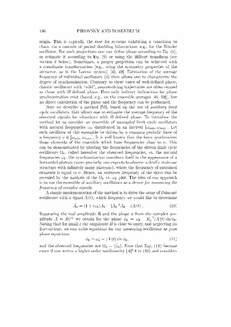
196 PIKOVSKY AND ROSENBLUM
origin. This is typically the case for systems exhibiting a transition to
chaos via a cascade of period doubling bifurcations; e.g., for the Rossler
oscillator. For such projections one can dene phase according to Eq. (8),
or estimate it according to Eq. (9) or using the Hilbert transform (see
section 8 below). Sometimes, a proper projection can be achieved with
a coordinate transformation (e.g., using the symmetry properties of the
attractor, as in the Lorenz system) [50, 49]. Estimation of the average
frequency of individual oscillators h _i then allows one to characterize the
degree of synchronization. Contrary to these cases of well-dened phase,
chaotic oscillators with \wild", non-revolving trajectories are often termed
as those with ill-dened phase. Here only indirect indications for phase
synchronization exist (based, e.g., on the ensemble averages [48, 50]), but
no direct calculation of the phase and the frequency can be performed.
Nere we describe a method [59], based on the use of auxiliary limitcycle oscillators, that allows one to estimate the average frequency of the
observed signals for situations with ill-dened phase. To introduce the
method let us consider an ensemble of uncoupled limit cycle oscillators
with natural frequencies !k distributed in an interval [!min; !max]. Let
each oscillator of this ensemble be driven by a common periodic force of
a frequency 2 [!min; !max]. It is well-known that the force synchronizes
those elements of the ensemble which have frequencies close to . This
can be demonstrated by plotting the frequencies of the driven limit cycle
oscillators k, called hereafter the observed frequencies, vs. the natural
frequencies !k: the synchronization manifests itself in the appearance of a
horizontal plateau (more precisely, one expects to observe a devil's staircase
structure with innitely many plateaus), where the frequency of entrained
elements is equal to . Hence, an unknown frequency of the drive can be
revealed by the analysis of the k vs. !k plot. The idea of our approach
is to use the ensemble of auxiliary oscillators as a device for measuring thefrequency of complex signals.
A simple implementation of the method is to drive the array of Poincare
oscillators with a signal X(t), which frequency we would like to determine
_Ak = (1 + i!k)Ak jAkj2Ak + "X(t) : (10)
Separating the real amplitude R and the phase from the complex am-
plitude A = Rei we obtain for the phase _k = !k R1k"X(t) sink.
Noting that for small " the amplitude R is close to unity, and neglecting its
uctuations, we can write equations for our measuring oscillators as pure
phase equations:_k = !k "X(t) sink; (11)
and the observed frequencies are k = h _ki. Note that Eqs. (11) become
exact if one writes a higher order nonlinearity jAjpA in (10) and considers
PHASE SYNCHRONIZATION 197
the limit p ! 1. In calculations below we normalize the signal X(t) to
have zero mean and unit variance so that the coupling constant " is the
only parameter of the method (the mean value can slightly in uence the
result).
To show how the method works we consider a model quasiharmonic
process with mean frequency !0 and slowly varying amplitude and phase:
X(t) = 2(1 + a(t)) cos(!0t (t)). Substituting this in (11) and averaging
over the period of fast oscillations 2=!0, we obtain for the slowly varying
phase dierence = !0t+ the equation
_ = ! !0 + _(t) "(1 + a(t)) sin ;
for a harmonic signal ( _ = a = 0) it has for " j! !0j the synchronizedsolution 0 = arcsin ((! !0)="). For weak modulation we can linearize
around this state and obtain for the deviations Æ :
d(Æ )
dt= _ a(t)(! !0)
p"2 (! !0)2Æ :
Assuming that and a are independent random processes, we can express
the power spectrum of the phase uctuations through the spectra of these
processes:
SÆ () =2S() + (! !0)
2Sa()
"2 (! !0)2 + 2:
One can see that the uctuations are small only in the middle of the
synchronization region (for ! !0); here only the phase uctuations Scontribute. Modeling S by the Lorentz-like spectrum
S =2V
(2 +2);
where V and are the variance and the characteristic maximal frequency
of uctuations of , we obtain
VÆ =
Z1
0
SÆ ()d = V("+)1 :
This nal formula shows that good synchronization (i.e. small variance of
Æ ) can be achieved if " is suÆciently larger than , i.e. if the coupling
constant is larger than the characteristic frequency of phase uctuations.
From the other side, in the limit " ! 1 the dependence of the observed
frequency on the natural one disappears, and the measured frequency is
the Rice frequency of the process X(t).
198 PIKOVSKY AND ROSENBLUM
−10 0 10x
−10
0
10y
0 1 2 3 4 5ω−1
1
3
5
log 10
S(ω
)
0.5 1.0 1.51
3(a) (b)
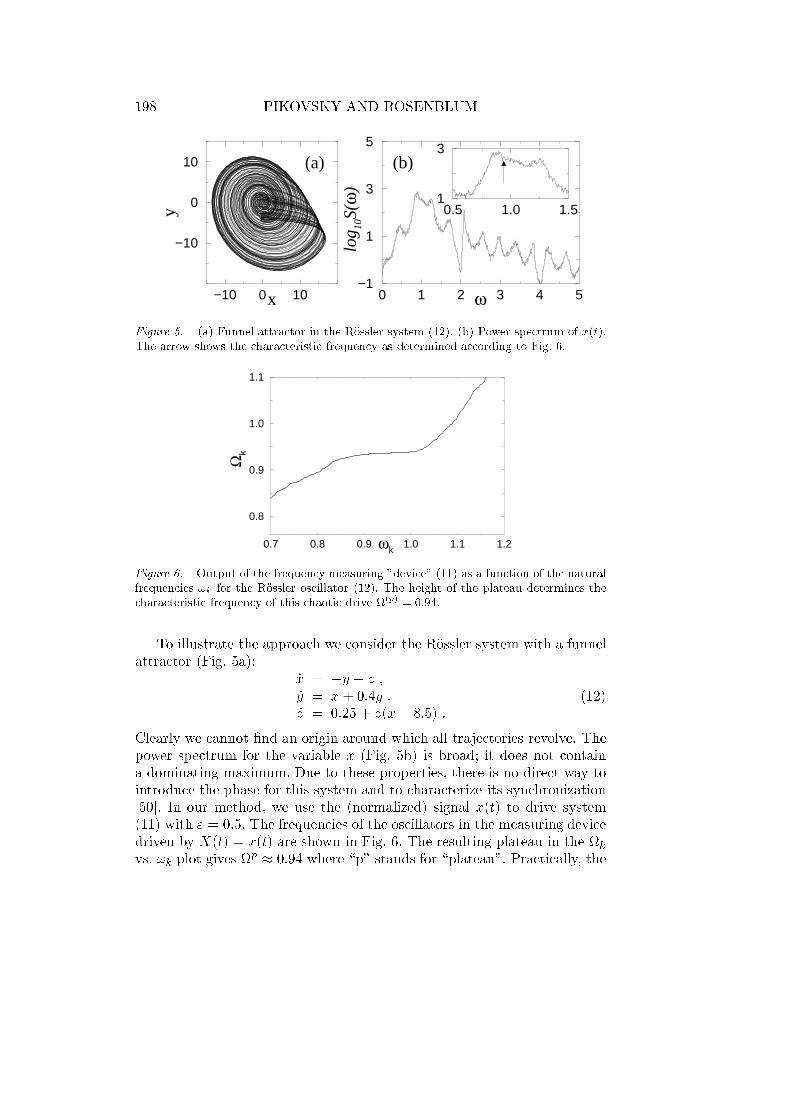
Figure 5. (a) Funnel attractor in the Rossler system (12). (b) Power spectrum of x(t).
The arrow shows the characteristic frequency as determined according to Fig. 6.
0.7 0.8 0.9 1.0 1.1 1.2ωk
0.8
0.9
1.0
1.1
Ωk
Figure 6. Output of the frequency measuring "device" (11) as a function of the natural
frequencies !k for the Rossler oscillator (12). The height of the plateau determines the
characteristic frequency of this chaotic drive (p) = 0:94.
To illustrate the approach we consider the Rossler system with a funnel
attractor (Fig. 5a):
_x = y z ;
_y = x+ 0:4y ;
_z = 0:25 + z(x 8:5) :(12)
Clearly we cannot nd an origin around which all trajectories revolve. The
power spectrum for the variable x (Fig. 5b) is broad; it does not contain
a dominating maximum. Due to these properties, there is no direct way to
introduce the phase for this system and to characterize its synchronization
[50]. In our method, we use the (normalized) signal x(t) to drive system
(11) with " = 0:5. The frequencies of the oscillators in the measuring device
driven by X(t) = x(t) are shown in Fig. 6. The resulting plateau in the kvs. !k plot gives
p 0:94 where \p" stands for \plateau". Practically, the
PHASE SYNCHRONIZATION 199
middle point of the plateau p
kwas determined from the minimum of the
running varianceP
k+Lj=kL(j k)
2, where k = (2L + 1)1P
k+Lj=kLj.
Variation of L from 3 to 10 gave no essential dierence. This method
provides also a smoothening of the k vs. !k curve. One can see that this
characteristic frequency cannot be directly associated with a peak in the
power spectrum (Fig. 5b). We also see that Fig. 6 does not show the devil's
staircase structure, but only one, smeared plateau. This is due to the chaotic
nature of the process x(t), so that, similar to the case of narrow-band noisy
signals, the high-order phase-locked regions are not observed [37, 49].
3.3. DYNAMICS OF THE PHASE OF CHAOTIC OSCILLATIONS
In contrast to the dynamics of the phase of periodic oscillations, the growth
of the phase in the chaotic case cannot generally be expected to be uniform.
Instead, the instantaneous frequency depends in general on the amplitude.
Let us hold to the phase denition based on the Poincare map, so one can
represent the dynamics as (cf. [52])
An+1 =M(An) ; (13)
d
dt= !(An) !0 + F (An) : (14)
As the amplitude A we take the set of coordinates for the point on the
secant surface; it does not change during the growth of the phase from
0 to 2 and can be considered as a discrete variable; the transformation
M denes the Poincare map. The phase evolves according to (14), where
the \instantaneous" frequency ! = 2=(tn+1 tn) depends in general on
the amplitude. Assuming the chaotic behavior of the amplitudes, we can
consider the term !(An) as a sum of the averaged frequency !0 and of
some eective noise F (A); in exceptional cases F (A) may vanish. For the
Rossler attractor the \period" of the rotations (i.e. the function 2=!(An))
is shown in Fig. 4(c). This period is not constant, so the function F (A)
does not vanish, but the variations of the period are relatively small.
Hence, the Eq. (14) is similar to the equation describing the evolution
of phase of periodic oscillator in the presence of external noise. Thus, the
dynamics of the phase is generally diusive: for large t one expects
h((t) (0) !0t)2i / Dpt ;
where the diusion constant Dp determines the phase coherence of the
chaotic oscillations. Roughly speaking, the diusion constant is propor-
tional to the width of the spectral peak calculated for the chaotic observable
[21].
200 PIKOVSKY AND ROSENBLUM
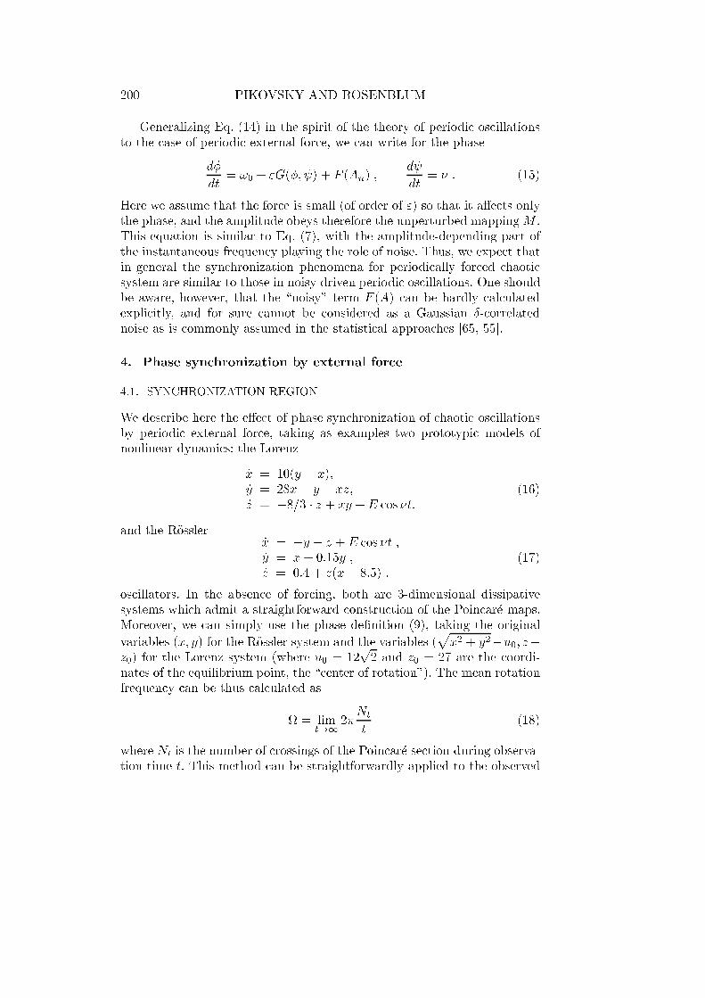
Generalizing Eq. (14) in the spirit of the theory of periodic oscillations
to the case of periodic external force, we can write for the phase
d
dt= !0 + "G(; ) + F (An) ;
d
dt= : (15)
Here we assume that the force is small (of order of ") so that it aects only
the phase, and the amplitude obeys therefore the unperturbed mappingM .
This equation is similar to Eq. (7), with the amplitude-depending part of
the instantaneous frequency playing the role of noise. Thus, we expect that
in general the synchronization phenomena for periodically forced chaotic
system are similar to those in noisy driven periodic oscillations. One should
be aware, however, that the \noisy" term F (A) can be hardly calculated
explicitly, and for sure cannot be considered as a Gaussian Æ-correlated
noise as is commonly assumed in the statistical approaches [65, 55].
4. Phase synchronization by external force
4.1. SYNCHRONIZATION REGION
We describe here the eect of phase synchronization of chaotic oscillations
by periodic external force, taking as examples two prototypic models of
nonlinear dynamics: the Lorenz
_x = 10(y x);
_y = 28x y xz;
_z = 8=3 z + xy +E cos t:
(16)
and the Rossler_x = y z +E cos t ;
_y = x+ 0:15y ;
_z = 0:4 + z(x 8:5) :(17)
oscillators. In the absence of forcing, both are 3-dimensional dissipative
systems which admit a straightforward construction of the Poincare maps.
Moreover, we can simply use the phase denition (9), taking the original
variables (x; y) for the Rossler system and the variables (px2 + y2u0; z
z0) for the Lorenz system (where u0 = 12p2 and z0 = 27 are the coordi-
nates of the equilibrium point, the \center of rotation"). The mean rotation
frequency can be thus calculated as
= limt!1
2Nt
t(18)
where Nt is the number of crossings of the Poincare section during observa-
tion time t. This method can be straightforwardly applied to the observed

PHASE SYNCHRONIZATION 201
0.90.95
11.05
1.11.15
ν 0.2
0.4
0.6
0.8
1
E
-0.1
0
0.1
0.2
ν−Ω (a)
8.28.25
8.38.35
8.48.45
8.5ν 0
24
68
1012
E
-0.15
-0.1
-0.05
0
0.05
0.1
0.15
0.2
ν−Ω (b)
Figure 7. The phase synchronization regions for the Rossler (a) and the Lorenz (b)
systems.
202 PIKOVSKY AND ROSENBLUM
time series, in the simplest case one can, e.g., take for Nt the number of
maxima (of x(t) for the Rossler system and of z(t) for the Lorenz one).
Dependence of the frequency obtained in this way on the amplitude
and frequency of the external force is shown in Fig. 7. Synchronization here
corresponds to the plateau = . One can see that the synchronization
properties of these two systems dier essentially. For the Rossler system
there exists a well-expressed region where the systems are perfectly locked.
Moreover, there seems to be no amplitude threshold of synchronization
(cf. Fig. 1c, where the phase-locking regions start at " = 0). It appears
that the phase locking properties of the Rossler system are practically the
same as for a periodic oscillator. On the contrary, for the Lorenz system
we observe the frequency locking only as a tendency seen at relatively large
forcing amplitudes, as this should be expected for oscillators subject to
a rather strong noise. In this respect, the dierence between Rossler and
Lorenz systems can be described in terms of phase diusion properties (see
Sect. 3.3). Indeed, the phase diusion coeÆcient for autonomous Rossler
system is extremely small Dp < 104, whereas for the Lorenz system it
is several oder of magnitude larger, Dp 0:2 [50]. This dierence in the
coherence of the phase of autonomous oscillations implies dierent response
to periodic forcing.
In the following sections we discuss the phase synchronization of chaotic
oscillations from the statistical and the topological viewpoints.
4.2. STATISTICAL APPROACH
We dene the phase of an autonomous chaotic system as a variable that
corresponds to the zero Lyapunov exponent, i.e. to the invariance with
respect to time shifts. Therefore, the invariant probability distribution as a
function of the phase is nearly uniform. This follows from the ergodicity of
the system: the probability is proportional to the time a trajectory is spend-
ing in a region of the phase space, and according to the denition (8) the
phase motion is (piecewise) uniform. With external forcing, the invariant
measure depends explicitly on time. In the synchronization region we expect
that the phase of oscillations nearly follows the phase of the force, while
without synchronization there is no denite relation between them. Let
us observe the oscillator stroboscopically, at the moments corresponding to
some phase 0 of the external force. In the synchronous state the probability
distribution of the oscillator phase will be localized near some preferable
value (which of course depends on the choice of 0). In the non-synchronous
state the phase is spread along the attractor. We illustrate this behavior of
the probability density in Fig. 8. One can say that synchronization means
localization of the probability density near some preferable time-periodic
state. In other words, this means appearance of the long-range correlation
PHASE SYNCHRONIZATION 203
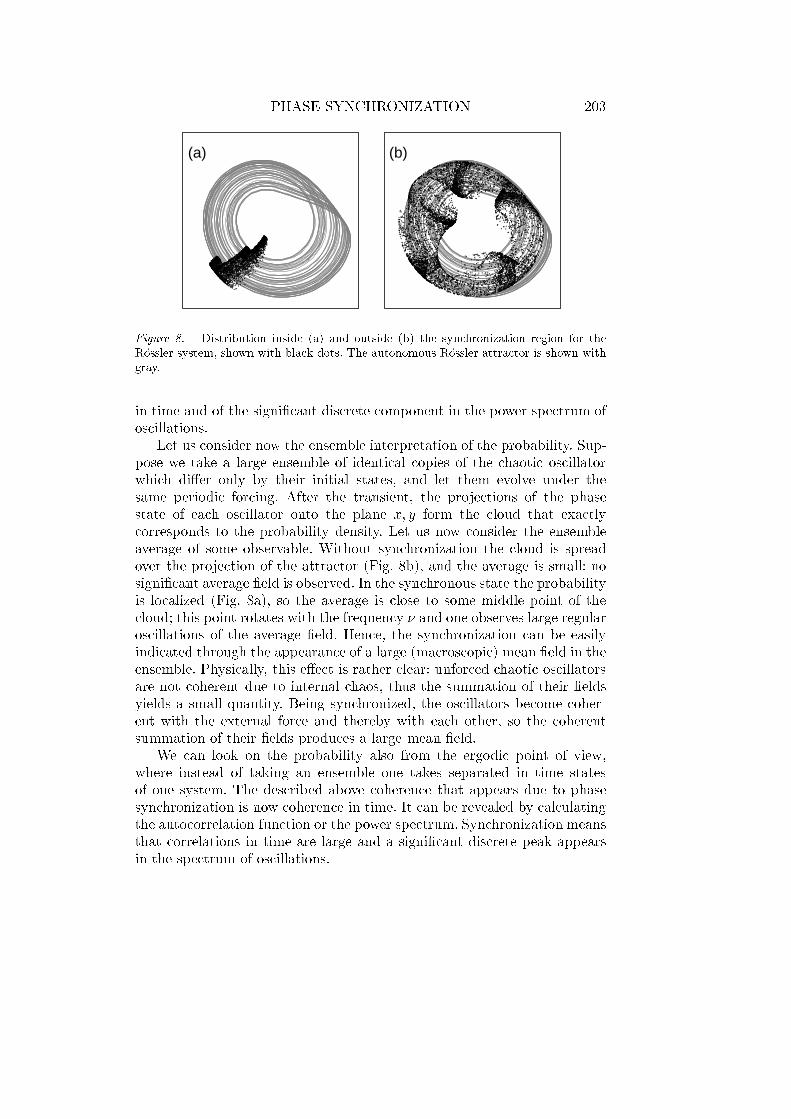
(a) (b)
Figure 8. Distribution inside (a) and outside (b) the synchronization region for the
Rossler system, shown with black dots. The autonomous Rossler attractor is shown with
gray.
in time and of the signicant discrete component in the power spectrum of
oscillations.
Let us consider now the ensemble interpretation of the probability. Sup-
pose we take a large ensemble of identical copies of the chaotic oscillator
which dier only by their initial states, and let them evolve under the
same periodic forcing. After the transient, the projections of the phase
state of each oscillator onto the plane x; y form the cloud that exactly
corresponds to the probability density. Let us now consider the ensemble
average of some observable. Without synchronization the cloud is spread
over the projection of the attractor (Fig. 8b), and the average is small: no
signicant average eld is observed. In the synchronous state the probability
is localized (Fig. 8a), so the average is close to some middle point of the
cloud; this point rotates with the frequency and one observes large regular
oscillations of the average eld. Hence, the synchronization can be easily
indicated through the appearance of a large (macroscopic) mean eld in the
ensemble. Physically, this eect is rather clear: unforced chaotic oscillators
are not coherent due to internal chaos, thus the summation of their elds
yields a small quantity. Being synchronized, the oscillators become coher-
ent with the external force and thereby with each other, so the coherent
summation of their elds produces a large mean eld.
We can look on the probability also from the ergodic point of view,
where instead of taking an ensemble one takes separated in time states
of one system. The described above coherence that appears due to phase
synchronization is now coherence in time. It can be revealed by calculating
the autocorrelation function or the power spectrum. Synchronization means
that correlations in time are large and a signicant discrete peak appears
in the spectrum of oscillations.
204 PIKOVSKY AND ROSENBLUM
An important consequence of the statistical approach described above
is that the phase synchronization can be characterized without explicit
computation of the phase and/or the mean frequency: it can be indicated
implicitly by the appearance of a macroscopic mean eld in the ensemble
of oscillators, or by the appearance of the large discrete component in
the spectrum. Although there may be other mechanisms leading to the
appearance of macroscopic order, the phase synchronization appears to be
one of the most common ones.
5. Phase synchronization in coupled systems
Now we demonstrate the eects of phase synchronization in coupled chaotic
oscillators. We start with the simplest case of two interacting systems,
and then brie y discuss oscillator lattices, globally coupled systems, and
space-time chaos.
5.1. SYNCHRONIZATION OF TWO INTERACTING OSCILLATORS
We consider here two non-identical coupled Rossler systems
_x1;2 = !1;2y1;2 z1;2 + "(x2;1 x1;2);
_y1;2 = !1;2x1;2 + ay1;2;
_z1;2 = f + z1;2(x1;2 c);
(19)
where a = 0:165, f = 0:2, c = 10. The parameters !1;2 = !0 !
and " determine the mismatch of natural frequencies and the coupling,
respectively.
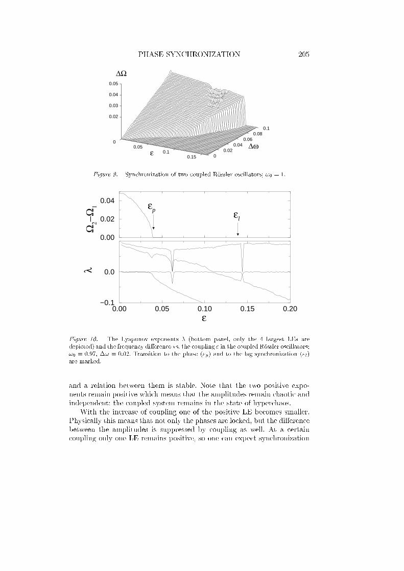
Again, like in the case of periodic forcing, we can dene the mean fre-
quencies 1;2 of oscillations of each system, and study the dependence of the
frequency mismatch 2 1 on the parameters !; ". This dependence is
shown in Fig. 9 and demonstrates a large region of synchronization between
two oscillators.
It is instructive to characterize the synchronization transition by means
of the Lyapunov exponents (LE). The 6-order dynamical system (19) has
6 LEs (see Fig. 10). For zero coupling we have a degenerate situation of
two independent systems, each of them has one positive, one zero, and
one negative exponent. The two zero exponents correspond to the two
independent phases. With coupling, the phases become dependent and the
degeneracy must be removed: only one LE should remain exactly zero. We
observe, however, that for small coupling also the second zero Lyapunov
exponent remains extremely small (in fact, numerically indistinguishable
from zero). Only at relatively stronger coupling, when the synchronization
sets on, the second LE becomes negative: now the phases are dependent
PHASE SYNCHRONIZATION 205
00.05
0.10.15 0
0.020.04
0.060.08
0.1
0.02
0.03
0.04
0.05
ε∆ω
∆Ω
Figure 9. Synchronization of two coupled Rossler oscillators; !0 = 1.
0.00 0.05 0.10 0.15 0.20ε
−0.1
0.0λ
0.00
0.02
0.04
Ω2−
Ω1 εp εl
Figure 10. The Lyapunov exponents (bottom panel, only the 4 largest LEs are
depicted) and the frequency dierence vs. the coupling " in the coupled Rossler oscillators;
!0 = 0:97, ! = 0:02. Transition to the phase ("p) and to the lag synchronization ("l)
are marked.
and a relation between them is stable. Note that the two positive expo-
nents remain positive which means that the amplitudes remain chaotic and
independent: the coupled system remains in the state of hyperchaos.
With the increase of coupling one of the positive LE becomes smaller.
Physically this means that not only the phases are locked, but the dierence
between the amplitudes is suppressed by coupling as well. At a certain
coupling only one LE remains positive, so one can expect synchronization
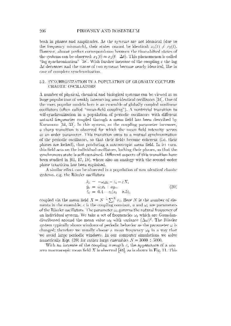
206 PIKOVSKY AND ROSENBLUM
both in phases and amplitudes. As the systems are not identical (due to
the frequency mismatch), their states cannot be identical: x1(t) 6= x2(t).
However, almost perfect correspondence between the time-shifted states of
the systems can be observed: x1(t) x2(tt). This phenomenon is called
\lag synchronization" [58]. With further increase of the coupling " the lag
t decreases and the states of two systems become nearly identical, like in
case of complete synchronization.
5.2. SYNCHRONIZATION IN A POPULATION OF GLOBALLY COUPLED
CHAOTIC OSCILLATORS
A number of physical, chemical and biological systems can be viewed at as
large populations of weakly interacting non-identical oscillators [34]. One of
the most popular models here is an ensemble of globally coupled nonlinear
oscillators (often called \mean-eld coupling"). A nontrivial transition to
self-synchronization in a population of periodic oscillators with dierent
natural frequencies coupled through a mean eld has been described by
Kuramoto [34, 33]. In this system, as the coupling parameter increases,
a sharp transition is observed for which the mean eld intensity serves
as an order parameter. This transition owes to a mutual synchronization
of the periodic oscillators, so that their elds become coherent (i.e. their
phases are locked), thus producing a macroscopic mean eld. In its turn,
this eld acts on the individual oscillators, locking their phases, so that the
synchronous state is self-sustained. Dierent aspects of this transition have
been studied in [61, 17, 18], where also an analogy with the secondorder
phase transition has been exploited.
A similar eect can be observed in a population of non-identical chaoticsystems, e.g. the Rossler oscillators
_xi = !iyi zi + "X;
_yi = !ixi + ayi;
_zi = 0:4 + zi(xi 8:5);
(20)
coupled via the mean eld X = N1P
N
1 xi. Here N is the number of ele-
ments in the ensemble, " is the coupling constant, a and !i are parameters
of the Rossler oscillators. The parameter !i governs the natural frequency of
an individual system. We take a set of frequencies !i which are Gaussian-
distributed around the mean value !0 with variance (!)2. The Rossler
system typically shows windows of periodic behavior as the parameter ! is
changed; therefore we usually choose a mean frequency !0 in a way that
we avoid large periodic windows. In our computer simulations we solve
numerically Eqs. (20) for rather large ensembles N = 3000 5000.
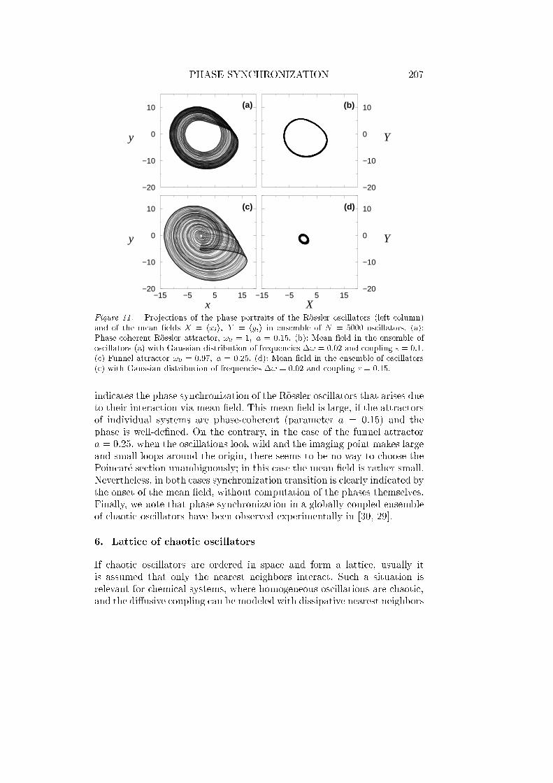
With an increase of the coupling strength ", the appearance of a non-
zero macroscopic mean eld X is observed [48], as is shown in Fig. 11. This
PHASE SYNCHRONIZATION 207
−15 −5 5 15x
−20
−10
0
10
y
−20
−10
0
10
y
(a) (b)
(c) (d)
−15 −5 5 15X
−20
−10
0
10
Y
−20
−10
0
10
Y
Figure 11. Projections of the phase portraits of the Rossler oscillators (left column)
and of the mean elds X = hxii; Y = hyii in ensemble of N = 5000 oscillators. (a):
Phase-coherent Rossler attractor, !0 = 1; a = 0:15. (b): Mean eld in the ensemble of
oscillators (a) with Gaussian distribution of frequencies ! = 0:02 and coupling " = 0:1.
(c) Funnel attractor !0 = 0:97; a = 0:25. (d): Mean eld in the ensemble of oscillators
(c) with Gaussian distribution of frequencies ! = 0:02 and coupling " = 0:15.
indicates the phase synchronization of the Rossler oscillators that arises due
to their interaction via mean eld. This mean eld is large, if the attractors
of individual systems are phase-coherent (parameter a = 0:15) and the
phase is well-dened. On the contrary, in the case of the funnel attractor
a = 0:25, when the oscillations look wild and the imaging point makes large
and small loops around the origin, there seems to be no way to choose the
Poincare section unambiguously; in this case the mean eld is rather small.
Nevertheless, in both cases synchronization transition is clearly indicated by
the onset of the mean eld, without computation of the phases themselves.
Finally, we note that phase synchronization in a globally coupled ensemble
of chaotic oscillators have been observed experimentally in [30, 29].
6. Lattice of chaotic oscillators
If chaotic oscillators are ordered in space and form a lattice, usually it
is assumed that only the nearest neighbors interact. Such a situation is
relevant for chemical systems, where homogeneous oscillations are chaotic,
and the diusive coupling can be modeled with dissipative nearest neighbors
208 PIKOVSKY AND ROSENBLUM
(a)
yj/Aj
0 25 50 75 1000
50
100
150
200
250
300
350
400
space
time
(b)
yj/Aj
0 25 50 75 1000
50
100
150
200
250
300
350
400
space
time
phase gradient
0 25 50 75 100space
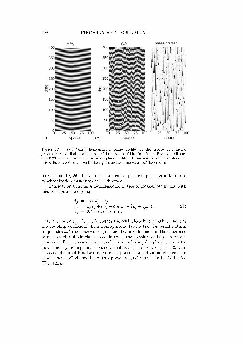
Figure 12. (a): Nearly homogeneous phase prole for the lattice of identical
phase-coherent Rossler oscillators. (b) In a lattice of identical funnel Rossler oscillators
a = 0:23, " = 0:05 an inhomogeneous phase prole with numerous defects is observed.
The defects are clearly seen in the right panel as large values of the gradient
interaction [10, 26]. In a lattice, one can expect complex spatio-temporal
synchronization structures to be observed.
Consider as a model a 1-dimensional lattice of Rossler oscillators with
local dissipative coupling:
_xj = !jyj zj ;
_yj = !jxj + ayj + "(yj+1 2yj + yj1);
_zj = 0:4 + (xj 8:5)zj :
(21)
Here the index j = 1; : : : ; N counts the oscillators in the lattice and " is
the coupling coeÆcient. In a homogeneous lattice (i.e. for equal natural
frequencies !j) the observed regime signicantly depends on the coherence
properties of a single chaotic oscillator. If the Rossler oscillator is phase-
coherent, all the phases nearly synchronize and a regular phase pattern (in
fact, a nearly homogeneous phase distribution) is observed (Fig. 12a). In
the case of funnel Rossler oscillator the phase at a individual element can
\spontaneously" change by , this prevents synchronization in the lattice
(Fig. 12b).
PHASE SYNCHRONIZATION 209
yj/Aj
0
200
400
600
800tim
eSj Aj
0 25 50j
1.0
1.2
1.4
Ωj
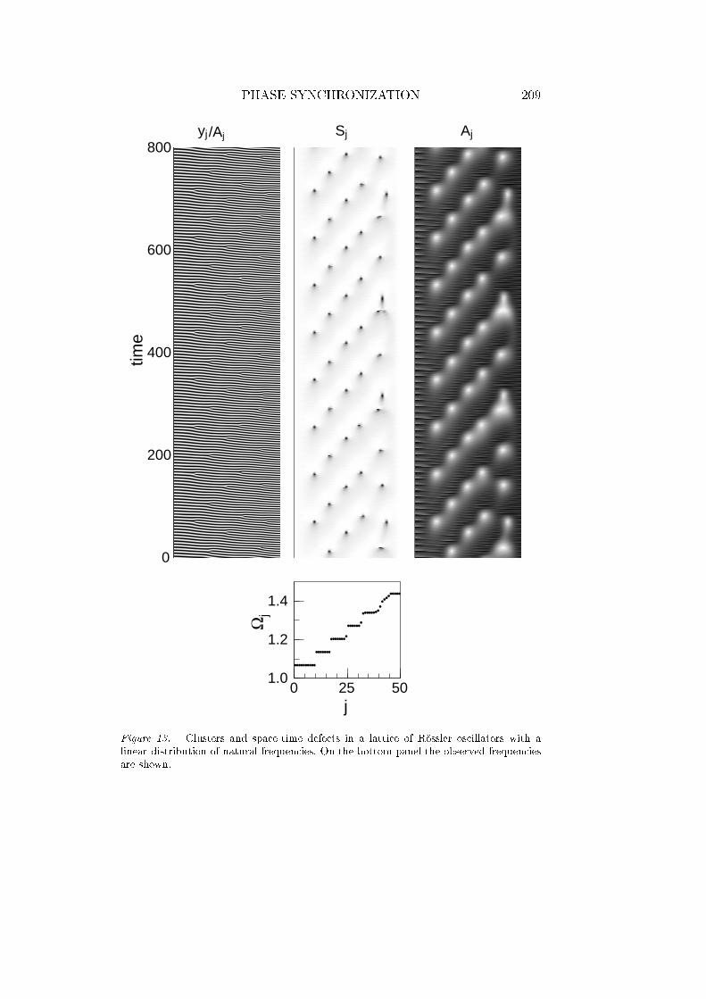
Figure 13. Clusters and space-time defects in a lattice of Rossler oscillators with a
linear distribution of natural frequencies. On the bottom panel the observed frequencies
are shown.
210 PIKOVSKY AND ROSENBLUM
To study synchronization in a lattice of non-identical oscillators, we
introduce a linear distribution of natural frequencies !j
!j = !1 + Æ(j 1) (22)
where Æ is the frequency mismatch between neighboring sites. Depending
on the values of Æ we observed two scenarios of transition to synchronization
[42]. For small Æ, the transition occurs smoothly, i.e. all the elements along
the chain gradually adjust their frequencies. If the frequency mismatch
is larger, clustering is observed: the oscillators build phase-synchronized
groups having dierent mean frequencies (Fig. 13). At the borders between
clusters phase slips occur; this can be considered as appearance of defects
in the spatio-temporal representation. Both regular and irregular patterns
of defects can be seen in Fig. 13.
7. Synchronization of space-time chaos
The idea of phase synchronization can be also applied to space-time chaos.
For example, in the famous complex Ginzburg-Landau equation (CGLE) [16,
13, 63]
@ta = (1 + i!0)a (1 + i)jaj2a+ (1 + i)@2t a ; (23)
there are regimes where the complex amplitude a rotates with some mean
frequency, but these rotations are not regular: the phase deviates irregu-
larly in space and time (this regime is called \phase turbulence"). Another
regime, where the complex amplitude a not always rotates but experiences
space-time defects (the places where the absolute value of the amplitude
vanishes whereas the phase is not dened); this regime is analogous to
oscillations with ill-dened phase like in the funnel Rossler oscillator.
Let us now add periodic in time spatially homogeneous forcing of am-
plitude B and frequency !e. Transition into a reference frame rotating with
this external forcing (a! A a exp(i!et)) reduces Eq. (23) to
@tA = (1 + i)A (1 + i)jAj2A+ (1 + i)@2tA+B ; (24)
where = !0 !e is the frequency mismatch between the frequency of
the external force and the frequency of small oscillations. An analysis of
dierent regimes in the system (24) has been recently performed [14]. As
one can expect, a very strong force suppresses turbulence and the spatially
homogeneous periodic in time synchronous oscillations are observed, while
a small force has no signicant in uence on the turbulent state. A nontrivial
regime is observed for intermediate forcing: in some parameter range the
irregular uctuations of the phase are not completely suppressed but are
bounded: the whole system oscillates \in phase" with the external force
PHASE SYNCHRONIZATION 211
(a)
00.1
0.20.3
0.40.5
0.60.7
B -2.2-1.8
-1.4-1
-0.6-0.2
ν
-1
-0.5
0
0.5
1
Ω
(b)
00.1
0.20.3
0.40.5
0.60.7
B -2.2-1.8
-1.4-1
-0.6-0.2
ν
0
0.5
1
1.5
2
defect density
(c)
00.1
0.20.3
0.40.5
0.60.7
B -2.2
-1.8
-1.4
-1
-0.6
-0.2
ν
-0.1
0
0.1
0.2
0.3
0.4
Lyap. exp.
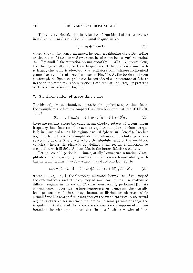
Figure 14. Synchronization of defect turbulence ( = 2, = 2): (a) Average frequency
as a function of the amplitude B and the frequency of the external force. The contour
lines are drawn at levels 0:5, 0:01, 0:01, 0:5. (b) Density of defects (arbitrary units).
The contour line shows the border of the defect-free region. (c) The largest Lyapunov
exponent. The contour line shows the border of the turbulent region.
and is highly coherent, although some small chaotic variations persist. In
Figs. 14,15 we show how the forcing acts on the regimes with defect and
phase turbulence in the CGLE. One can see that the forcing can supress
defects while not supressing completely the space-time chaos; this regime
is analogous to phase synchronization of individual oscillators. In the case
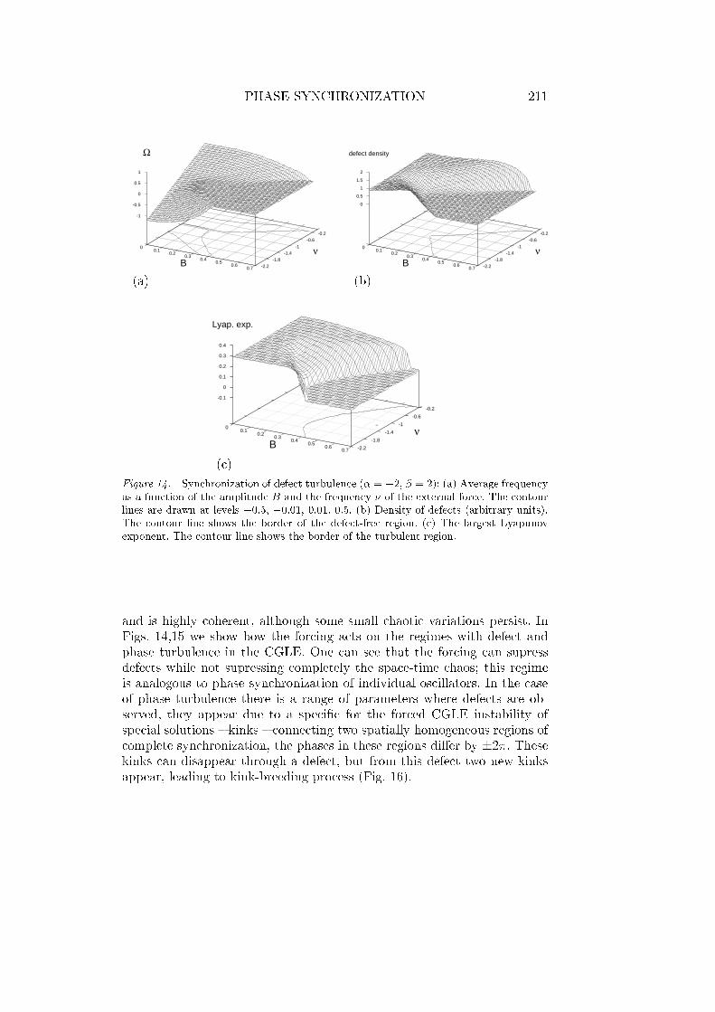
of phase turbulence there is a range of parameters where defects are ob-
served, they appear due to a specic for the forced CGLE instability of
special solutions kinks connecting two spatially homogeneous regions of
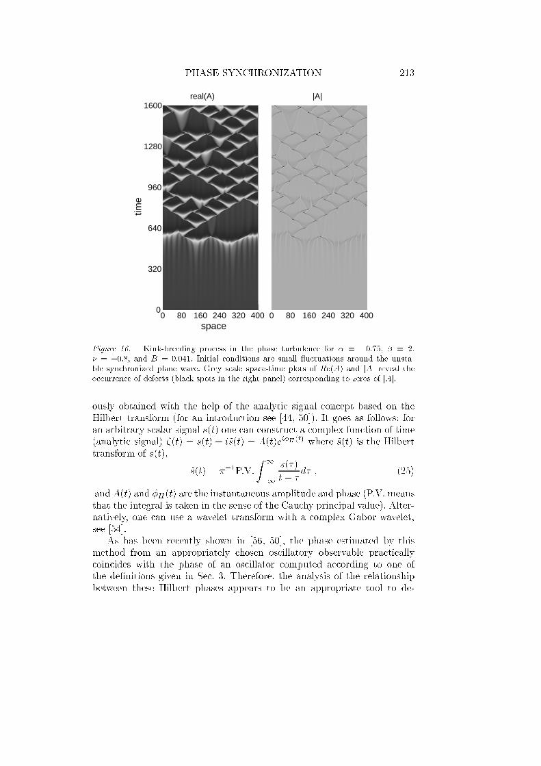
complete synchronization, the phases in these regions dier by 2. Thesekinks can disappear through a defect, but from this defect two new kinks
appear, leading to kink-breeding process (Fig. 16).
212 PIKOVSKY AND ROSENBLUM
(a)-0.8
-0.78
-0.76
-0.74
-0.72
-0.7
ν
00.01
0.020.03
0.040.05
0.060.07
0.08
B
-0.05
0
0.05
Ω
(b)-0.8
-0.78
-0.76
-0.74
-0.72
-0.7
ν
00.01
0.020.03
0.040.05
0.060.07
0.08
B
0
0.5
1
defect density
(c)-0.8
-0.78
-0.76
-0.74
-0.72
-0.7
ν
00.01
0.020.03
0.040.05
0.060.07
B
-0.04
-0.02
0
0.02
lyap exp
Figure 15. Synchronization of phase turbulence ( = 0:75, = 2). (a) The average
frequency as a function of the amplitude B and the frequency of the external force.
The contour line shows the border of the synchronization region. (b) The density of
defects (arbitrary units). (c) The largest Lyapunov exponent. The contour lines show the
borders between the regions of positive, zero, and negative exponents.
8. Detecting synchronization in data
The analysis of relation between the phases of two systems, naturally arising
in the context of synchronization, can be used to approach a general prob-
lem in time series analysis. Indeed, bivariate data are often encountered in
the study of real systems, and the usual aim of the analysis of such data is
to nd out whether two signals are dependent or not. As experimental data
are very often non-stationary, the traditional techniques, such as cross
spectrum and crosscorrelation analysis [44], or nonlinear characteristics
like generalized mutual information [53] or maximal correlation [71] have
their limitations. From the other side, sometimes it is reasonable to assume
that the observed signals originate from two weakly interacting systems.
The presence of this interaction can be found by means of the analysis
of instantaneous phases of these signals. These phases can be unambigu-
PHASE SYNCHRONIZATION 213
real(A)
0 80 160 240 320 4000
320
640
960
1280
1600
space
time
|A|
0 80 160 240 320 400
Figure 16. Kink-breeding process in the phase turbulence for = 0:75, = 2,
= 0:8, and B = 0:041. Initial conditions are small uctuations around the unsta-
ble synchronized plane wave. Grey scale space-time plots of Re(A) and jAj reveal theoccurrence of defects (black spots in the right panel) corresponding to zeros of jAj.
ously obtained with the help of the analytic signal concept based on the
Hilbert transform (for an introduction see [44, 50]). It goes as follows: for
an arbitrary scalar signal s(t) one can construct a complex function of time
(analytic signal) (t) = s(t) + i~s(t) = A(t)eiH (t) where ~s(t) is the Hilbert
transform of s(t),
~s(t) = 1P.V.
Z1
1
s()
t d ; (25)
andA(t) and H(t) are the instantaneous amplitude and phase (P.V. means
that the integral is taken in the sense of the Cauchy principal value). Alter-
natively, one can use a wavelet transform with a complex Gabor wavelet,
see [54].
As has been recently shown in [56, 50], the phase estimated by this
method from an appropriately chosen oscillatory observable practically
coincides with the phase of an oscillator computed according to one of
the denitions given in Sec. 3. Therefore, the analysis of the relationship
between these Hilbert phases appears to be an appropriate tool to de-
214 PIKOVSKY AND ROSENBLUM
tect synchronous epochs from experimental data and to check for a weak
interaction between systems under study. It is very important that the
Hilbert transform does not require stationarity of the data, so we can trace
synchronization transitions even from nonstationary data.
We recall again the above mentioned similarity of phase dynamics in
noisy and chaotic oscillators (see Sect. 3.3). A very important consequence
of this fact is that, using the synchronization approach to data analysis,
we can avoid the hardly solvable dilemma \noise vs chaos": irrespectively
of the origin of the observed signals, the approach and techniques of the
analysis are unique. Quantication of synchronization from noisy data is
considered in [67].
Application of these ideas allowed us to nd phase locking in the data
characterizing mechanisms of posture control in humans while quiet stand-
ing [60, 57]. Namely, the small deviations of the body center of gravity in
anteriorposterior and lateral directions were analyzed. In healthy subjects,
the regulation of posture in these two directions can be considered as
independent processes, and the occurrence of some interrelation possibly
indicates a pathology. It is noteworthy that in several records conventional
methods of time series analysis, i.e. the crossspectrum analysis and the
generalized mutual information failed to detect any signicant dependence
between the signals, whereas calculation of the instantaneous phases clearly
showed phase locking.
Complex synchronous patterns have been found recently in the analysis
of interaction of human cardiovascular and respiratory systems [62]. This
nding possibly indicates the existence of a previously unknown type of
neural coupling between these systems.
Analysis of synchronization between brain and muscle activity of a
Parkinsonian patient [67] is relevant for a fundamental problem of neu-
roscience: can one consider the synchronization between dierent areas of
the motor cortex as a necessary condition for establishing of the coordi-
nated muscle activity? It was shown [67] that the temporal evolution of
the coordinated pathologic tremor activity directly re ects the evolution of
the strength of synchronization within a neural network involving cortical
motor areas. Additionally, the brain areas with the tremor-related activity
were localized from noninvasive measurements.
9. Conclusions
The main idea of this paper is to demonstrate that synchronization phenom-
ena in periodic, noisy and chaotic oscillators can be understood within a
unied framework. This is achieved by extending the notion of phase to the
case of continuous-time chaotic systems. Because the phase is introduced as
PHASE SYNCHRONIZATION 215
a variable corresponding to the zero Lyapunov exponent, this notion should
be applicable to any autonomous chaotic oscillator. Although we are not
able to propose a unique and rigorous approach to determine the phase,
we have shown that it can be introduced in a reasonable and consistent
way for basic models of chaotic dynamics. Moreover, we have shown that
even in the case when the phases are not well-dened, i.e. they cannot be
unambiguously computed explicitly, the presence of phase synchronization
can be demonstrated indirectly by observations of the mean eld and the
spectrum, i.e. independently of any particular denition of the phase.
In a rather general framework, any type of synchronization can be con-
sidered as appearance of some additional order inside the dynamics. For
chaotic systems, e.g., the complete synchronization means that the dynam-
ics in the phase space is restricted to a symmetrical submanifold. Thus, from
the point of view of topological properties of chaos, the synchronization
transition usually means the simplication of the structure of the strange
attractor. In discussing the topological properties of phase synchronization,
we have shown that the transition to phase synchronization corresponds
to splitting of the complex invariant chaotic set into distinctive attractor
and repeller. Analogously to the complete synchronization, which appears
through the pitchfork bifurcation of the strange attractor, one can say that
the phase synchronization appears through tangent bifurcation of strange
sets.
Because of the similarity in the phase dynamics, one may expect that
many, if not all, synchronization features known for periodic oscillators can
be observed for chaotic systems as well. Indeed, here we have described
eects of phase and frequency entrainment by periodic external driving,
both for simple and space-distributed chaotic systems. Further, we have
described synchronization due to interaction of two chaotic oscillators, as
well as self-synchronization in globally coupled large ensembles.
As an application of the developed framework we have discussed a
problem in data analysis, namely detection of weak interaction between
systems from bivariate data. The three described examples of the analysis
of physiological data demonstrate a possibility to detect and characterize
synchronization even from nonstationary and noisy data.
Finally, we would like to stress that contrary to other types of chaotic
synchronization, the phase synchronization phenomena can happen already
for very weak coupling, which oers an easy way of chaos regulation.
Acknowledgements
We thank M. Zaks, J. Kurths, G. Osipov, H. Chate, O. Rudzick, U. Parlitz,
P. Tass, C. Schafer for useful discussions.
216 PIKOVSKY AND ROSENBLUM
References
1. Andronov, A. A. and A. A. Vitt: 1930a, `On mathematical theory of entrainment'.
Zhurnal prikladnoi ziki (J. Appl. Phys.) 7(4), 3. (In Russian).
2. Andronov, A. A. and A. A. Vitt: 1930b, `Zur Theorie des Mitnehmens von van der
Pol'. Archiv fur Elektrotechnik 24(1), 99110.
3. Appleton, E. V.: 1922, `The Automatic Synchronization of Triode Oscillator'. Proc.
Cambridge Phil. Soc. (Math. and Phys. Sci.) 21, 231248.
4. Arnold, V. I.: 1961, `Small denominators. I. Mappings of the circumference onto
itself'. Izv. Akad. Nauk Ser. Mat. 25(1), 2186. (In Russian); English Translation:
AMS Transl. Ser. 2, v. 46, 213-284.
5. Berge, P., Y. Pomeau, and C. Vidal: 1986, Order within chaos. New York: Wiley.
6. Bezaeva, L., L. Kaptsov, and P. S. Landa: 1987, `Synchronization Threshold as the
Criterium of Stochasticity in the Generator with Inertial Nonlinearity'. Zhurnal
Tekhnicheskoi Fiziki 32, 467650. (In Russian).
7. Blekhman, I. I.: 1971, Synchronization of Dynamical Systems. Moscow: Nauka. (In
Russian).
8. Blekhman, I. I.: 1981, Synchronization in Science and Technology. Moscow: Nauka.
(In Russian); English translation: 1988, ASME Press, New York.
9. Bremsen, A. S. and I. S. Feinberg: 1941, `Analysis of functioning of two coupled
relaxtion generators'. Zhurnal Technicheskoi Fiziki (J. Techn. Phys.) 11(10). (In
Russian).
10. Brunnet, L., H. Chate, and P. Manneville: 1994, `LongRange Order with Local
Chaos in Lattices of Diusively Coupled ODEs'. Physica D 78, 141154.
11. Cartwright, M. L.: 1948, `Forced oscillations in nearly sinusoidal systems'. J. Inst.
Elec. Eng. 95, 88.
12. Cartwright, M. L. and J. E. Littlewood: 1945, `On nonlinear dierential equations
of the second order'. J. London Math. Soc. 20, 180189.
13. Chate, H.: 1994, `Spatiotemporal intermittency regimes of the one-dimensional
complex Ginzburg-Landau equation'. Nonlinearity 7, 185204.
14. Chate, H., A. Pikovsky, and O. Rudzick: 1999, `Forcing Oscillatory Media: Phase
Kinks vs. Synchronization'. Physica D 131(1-4), 1730.
15. Cornfeld, I. P., S. V. Fomin, and Y. G. Sinai: 1982, Ergodic Theory. New York:
Springer.
16. Cross, M. C. and P. C. Hohenberg: 1993, `Pattern formation outside of equilibrium'.
Rev. Mod. Phys. 65(3), 851.
17. Daido, H.: 1986, `Discrete-time population dynamics of interacting self-oscillators'.
Prog. Theor. Phys. 75(6), 14601463.
18. Daido, H.: 1990, `Intrinsic Fluctuations and a Phase Transition in a class of Large
Population of Interacting Oscillators'. J. Stat. Phys. 60(5/6), 753800.
19. Denjoy, A.: 1932, `Sur les courbes denes par les equations dierentielles a la syrface
du tore'. Jour. de Matheematiques Pures at Appliquees 11, 333375.
20. Dykman, G. I., P. S. Landa, and Y. I. Neymark: 1991, `Synchronizing the Chaotic
Oscillations by External Force'. Chaos, Solitons & Fractals 1(4), 339353.
21. Farmer, J. D.: 1981, `Spectral broadening of period-doubling bifurcation sequences'.
Phys. Rev. Lett 47(3), 179182.
22. Fujisaka, H. and T. Yamada: 1983, `Stability theory of synchronized motion in
coupled-oscillator systems'. Prog. Theor. Phys. 69(1), 3247.
23. Gaponov, V.: 1936, `Two coupled generators with soft self-excitation'. Zhurnal
Technicheskoi Fiziki (J. Techn. Phys.) 6(5). (In Russian).
PHASE SYNCHRONIZATION 217
24. Glass, L.: 2001, `Synchronization and rhythmic processes in physiology'. Nature
410, 277284.
25. Glass, L. and M. C. Mackey: 1988, From Clocks to Chaos: The Rhythms of Life.
Princeton, NJ: Princeton Univ. Press.
26. Goryachev, A. and R. Kapral: 1996, `Spiral waves in chaotic systems'. Phys. Rev.
Lett. 76(10), 16191622.
27. Huygens, C.: 1673, Horologium Oscillatorium. Parisiis, France: Apud F. Muguet.
English translation: The Pendulum Clock, Iowa State University Press, Ames, 1986.
28. Kiss, I. and J. Hudson: 2001, `Phase synchronization and suppression of chaos
through intermittency in forcing of an electrochemical oscillator'. Phys. Rev. E
64, 046215.
29. Kiss, I., Y. Zhai, and J. Hudson: 2002a, `Collective dynamics of chaotic chemical
oscillators and the law of large numbers'. Phys. Rev. Lett. 88(23), 238301.
30. Kiss, I., Y. Zhai, and J. Hudson: 2002b, `Emerging coherence in a population of
chemical oscillators'. Science 296, 16761678.
31. Kocarev, L. and U. Parlitz: 1995, `General approach for chaotic synchronization
with applications to communication'. Phys. Rev. Lett. 74(25), 50285031.
32. Kocarev, L., A. Shang, and L. O. Chua: 1993, `Transitions in dynamical regimes by
driving: a unied method of control and synchronization of chaos'. International
Journal of Bifurcation and Chaos 3(2), 479483.
33. Kuramoto, Y.: 1975, `Self-entrainment of a Population of Coupled Nonlinear Oscil-
lators'. In: H. Araki (ed.): International Symposium on Mathematical Problems in
Theoretical Physics. New York, p. 420.
34. Kuramoto, Y.: 1984, Chemical Oscillations, Waves and Turbulence. Berlin:
Springer.
35. Kurths, Editor, J.: 2000, `A focus issue on phase synchronization in chaotic systes'.
Int. J. Bifurcation and Chaos.
36. Kuznetsov, Y., P. S. Landa, A. Ol'khovoi, and S. Perminov: 1985, `Relationship
Between the Amplitude Threshold of Synchronization and the entropy in stochastic
selfexcited systems'. Sov. Phys. Dokl. 30(3), 221222.
37. Landa, P. S.: 1980, SelfOscillations in Systems with Finite Number of Degrees of
Freedom. Moscow: Nauka. (In Russian).
38. Landa, P. S. and M. G. Rosenblum: 1992, `Synchronization of Random Self
Oscillating Systems'. Sov. Phys. Dokl. 37(5), 237239.
39. Landa, P. S. and M. G. Rosenblum: 1993, `Synchronization and Chaotization of
Oscillations in Coupled SelfOscillating Systems'. Applied Mechanics Reviews 46(7),
414426.
40. Mandelshtam, L. and N. Papaleksi: 1947, `On the nth Kind Resonance Phenom-
ena'. In: Collected Works by L.I. Mandelshtam, Vol. 2. Moscow: Izd. Akademii
Nauk, pp. 1320. (in Russian).
41. Mayer, A.: 1935, `On the theory of coupled vibrations of two self-excited generators'.
Technical physics of the USSR 11.
42. Osipov, G., A. Pikovsky, M. Rosenblum, and J. Kurths: 1997, `Phase Synchroniza-
tion Eects in a Lattice of Nonidentical Rossler Oscillators'. Phys. Rev. E 55(3),
23532361.
43. Ott, E.: 1992, Chaos in Dynamical Systems. Cambridge: Cambridge Univ. Press.
44. Panter, P.: 1965,Modulation, Noise, and Spectral Analysis. New York: McGrawHill.
45. Parlitz, U., L. Junge, W. Lauterborn, and L. Kocarev: 1996, `Experimental
Observation of Phase Synchronization'. Phys. Rev. E. 54(2), 21152118.

218 PIKOVSKY AND ROSENBLUM
46. Pecora, L. M. and T. L. Carroll: 1990, `Synchronization in chaotic systems'. Phys.
Rev. Lett. 64, 821824.
47. Pecora, Editor, L.: 1997, `A focus issue on synchronization in chaotic systes'.
CHAOS.
48. Pikovsky, A., M. Rosenblum, and J. Kurths: 1996, `Synchronization in a Population
of Globally Coupled Chaotic Oscillators'. Europhys. Lett. 34(3), 165170.
49. Pikovsky, A., M. Rosenblum, and J. Kurths: 2001, Synchronization. A Universal
Concept in Nonlinear Sciences. Cambridge: Cambridge University Press.
50. Pikovsky, A., M. Rosenblum, G. Osipov, and J. Kurths: 1997, `Phase Synchroniza-
tion of Chaotic Oscillators by External Driving'. Physica D 104, 219238.
51. Pikovsky, A. S.: 1984, `On the interaction of strange attractors'. Z. Physik B 55(2),
149154.
52. Pikovsky, A. S.: 1985, `Phase synchronization of chaotic oscillations by a periodic
external eld'. Sov. J. Commun. Technol. Electron. 30, 85.
53. Pompe, B.: 1993, `Measuring Statistical Dependencies in a Time Series'. J. Stat.
Phys. 73, 587610.
54. Quian Quiroga, R., A. Kraskov, T. Kreuz, and P. Grassberger: 2002, `Per-
formance of dierent synchronization measures in real data: A case study on
electroencephalographic signals'. Phys. Rev. E 65, 041903.
55. Risken, H. Z.: 1989, The FokkerPlanck Equation. Berlin: Springer.
56. Rosenblum, M., A. Pikovsky, and J. Kurths: 1996, `Phase synchronization of chaotic
oscillators'. Phys. Rev. Lett. 76, 1804.
57. Rosenblum, M., A. Pikovsky, and J. Kurths: 1997a, `Eect of Phase Synchronization
in Driven and Coupled Chaotic Oscillators'. IEEE Trans. CAS-I 44(10), 874881.
58. Rosenblum, M., A. Pikovsky, and J. Kurths: 1997b, `From Phase to Lag Synchro-
nization in Coupled Chaotic Oscillators'. Phys. Rev. Lett. 78, 41934196.
59. Rosenblum, M., A. Pikovsky, J. Kurths, G. Osipov, I. Kiss, and J. Hudson: 2002,
`Locking-based frequency measurement and synchronization of chaotic oscillators
with complex dynamics'. Phys. Rev. Lett. 89(26), 264102.
60. Rosenblum, M. G., G. I. Firsov, R. A. Kuuz, and B. Pompe: 1998, `Human Postural
Control: Force Plate Experiments and Modelling'. In: H. Kantz, J. Kurths, and G.
Mayer-Kress (eds.): Nonlinear Analysis of Physiological Data. Berlin: Springer, pp.
283306.
61. Sakaguchi, H., S. Shinomoto, and Y. Kuramoto: 1987, `Local and global self-
entrainments in oscillator lattices'. Prog. Theor. Phys. 77(5), 10051010.
62. Schafer, C., M. G. Rosenblum, J. Kurths, and H.-H. Abel: 1998, `Heartbeat
Synchronized with Ventilation'. Nature 392(6673), 239240.
63. Shraiman, B. I., A. Pumir, W. van Saarlos, P. Hohenberg, H. Chate, and M. Holen:
1992, `Spatiotemporal Chaos in the One-dimensional Ginzburg-Landau equation'.
Physica D 57, 241248.
64. Stratonovich, R.: 1958, `Oscillator synchronization in the presence of noise'. Ra-
diotechnika i Elektronika 3(4), 497. (In Russian); English translation in: Non-
linear Transformations of Stochastic Processes, Edited by P.I. Kuznetsov, R.L.
Stratonovich and V.I. Tikhonov, Pergamon Press, Oxford London, 1965, pp.
269-282.
65. Stratonovich, R. L.: 1963, Topics in the Theory of Random Noise. New York: Gordon
and Breach.
66. Tang, D. Y. and N. R. Heckenberg: 1997, `Synchronization of Mutually Coupled
Chaotic Systems'. Phys. Rev. E 55(6), 66186623.
67. Tass, P., M. G. Rosenblum, J. Weule, J. Kurths, A. S. Pikovsky, J. Volkmann,
PHASE SYNCHRONIZATION 219
A. Schnitzler, and H.-J. Freund: 1998, `Detection of n : m Phase Locking from
Noisy Data: Application to Magnetoencephalography'. Phys. Rev. Lett. 81(15),
32913294.
68. Teodorchik, K.: 1943, `On the theory of synchronization of relaxational self-
oscillations'. Doklady Akademii Nauk SSSR (Sov. Phys. Dokl) 40(2), 63. (In
Russian).
69. Ticos, C. M., E. Rosa Jr., W. B. Pardo, J. A. Walkenstein, and M. Monti: 2000, `Ex-
perimental Real-Time Phase Synchronization of a Paced Chaotic Plasma Discharge'.
Phys. Rev. Lett. 85(14), 29292932.
70. van der Pol, B.: 1927, `Forced oscillators in a circuit with non-linear resistance.
(Reception with reactive triode)'. Phil. Mag. 3, 6480.
71. Voss, H. and J. Kurths: 1997, `Reconstruction of Nonlinear Time Delay Models from
Data by the Use of Optimal Transformations'. Phys. Lett. A 234, 336344.