Department of Economics and Finance

Working Paper No. 09-37

http://www.brunel.ac.uk/about/acad/sss/depts/economics

Econ

omic

s an

d Fi

nanc

e W

orki

ng P

aper

Ser

ies

Guglielmo Maria Caporale, Christophe Rault, Robert Sova and Anamaria Sova

Financial Development and Economic Growth: Evidence from Ten New EU Members

October 2009

Financial Development and Economic Growth:

Evidence from Ten New EU Members

Guglielmo Maria CAPORALE

Brunel University (London), CESifo and DIW Berlin

Christophe RAULT

LEO, University of Orleans and IZA

Robert SOVA

CES, Sorbonne University and ASE

Anamaria SOVA

CES, Sorbonne University and EBRC

October 2009

Abstract This paper reviews the main features of the banking and financial sector in ten new EU

members, and then examines the relationship between financial development and economic

growth in these countries by estimating a dynamic panel model over the period 1994-2007. The

evidence suggests that the stock and credit markets are still underdeveloped in these economies,

and that their contribution to economic growth is limited owing to a lack of financial depth. By

contrast, a more efficient banking sector is found to have accelerated growth. Furthermore,

Granger causality test indicate that causality runs from financial development to economic

growth, but not in the opposite direction.

Keywords: Financial Development, Economic Growth, Causality Tests, Transition Economies

JEL classification codes: E44, E58, F36, P26

Corresponding author: Professor Guglielmo Maria Caporale, Centre for Empirical Finance,

Brunel University, West London, UB8 3PH, UK. Tel.: +44 (0)1895 266713. Fax: +44 (0)1895

269770. Email: Guglielmo-Maria.Caporale@brunel.ac.uk

1 

 

1. Introduction

The relationship between financial development and economic growth has been extensively

analysed in the literature. Most empirical studies conclude that the former, together with a more

efficient banking system, accelerates the latter (Levine, 1997, 2005; Wachtel, 2001). Levine

(2005) suggests that financial institutions and markets can foster economic growth through

several channels, i.e. by (i) easing the exchange of goods and services through the provision of

payment services, (ii) mobilising and pooling savings from a large number of investors, (iii)

acquiring and processing information about enterprises and possible investment projects, thus

allocating savings to their most productive use, (iv) monitoring investment and carrying out

corporate governance, and (v) diversifying, increasing liquidity and reducing intertemporal risk.

Each of these functions can influence saving and investment decisions and hence economic

growth. Since many market frictions exist and laws, regulations, and policies differ markedly

across economies and over time, improvements along any single dimension may have different

implications for resource allocation and welfare depending on other frictions in the economy.

The reform of the financial sector in Central and Eastern Europe (CEE) started from the banking

sector. Its transformation has been one of the most important aspects of the transition process

from a centrally planned to a market economy. Initially a heavily regulated industry, the banking

system has been rapidly turned into one of the most dynamic sectors of the economy. The

process started in the early 1990s when foreign banks began investing in the region. From 2004,

these have been holding majority shares in all CEE countries. Their entry into the market has

resulted in considerable benefits for the sector and the economy in general, but they have had to

face various challenges deriving mostly from the underdevelopment of key institutional support

for banking growth.

Although accession to the European Union (EU) has helped the reform process in the CEE

countries, real convergence in terms of real GDP per capita remains a challenge. The present

study investigates whether financial development can be instrumental in reducing the gap vis-à-

vis the other EU members. Specifically, after reviewing the main features of the banking and

2 

 

financial sectors in these countries, it examines the empirical linkages between financial

development and economic growth by estimating a Barro–type growth regression augmented

with the inclusion of financial variables using panel data for ten transition countries over period

1994-2007. As financial development varies considerably across these countries, we split them

into three more homogenous groups: Central and Eastern European countries (CEE-5), Baltic

countries (B-3) and Southeastern European countries (SEE-2). We also consider the determinants

of credit, given its importance for financing investment projects and its impact on economic

growth. We analyse these issues by employing the system GMM method to control for

endogeneity and measurement errors and obtain unbiased, consistent and efficient estimates.

Finally, Granger causality tests are carried out.

The layout of the paper is the following. Section 2 provides a brief review of the literature on the

relationship between finance and growth. Section 3 analyses the evolution of the financial and

banking sector in ten transition economies. Section 4 discusses the data and the econometric

approach, as well as the panel evidence on the nexus between financial development and

economic growth. Section 5 carries out bi-directional causality tests between financial

development/efficiency of the banking system and economic growth. Section 6 offers some

concluding remarks.

2. Literature Review The relationship between financial development and economic growth is a controversial issue.

Some authors consider finance an important element of growth (Schumpeter, 1934; Goldsmith,

1969; McKinnon, 1973; Shaw, 1973; King and Levine (1993), whilst for others it is only a minor

growth factor (Robinson, 1952; Lucas, 1988). Schumpeter (1934) sees the banking sector as an

engine of economic growth through its funding of productive investment. On the contrary, Lucas

(1988) argues that the role of finance has been overstressed.

Greenwood and Jovanovic (1990) model the dynamic interactions between finance and growth

and emphasise the two-way causality between them. Financial intermediaries produce better

information and improve resource allocation. An expanded system of financial intermediation is

3 

 

able to allocate more capital to efficient investments and thus to foster economic growth.

Bencivenga and Smith (1991) highlight the fact that, by eliminating liquidity risk, banks can

raise economic growth. Financial intermediaries boost productivity, capital accumulation and

growth by improving corporate governance.

Existing studies typically focus on variables capturing the size, activity or efficiency of specific

financial institutions or markets. Early contributions used aggregate data on banks for a large

number of developed and developing countries including the ratio to GDP of monetary variables

(M2 or M3), or financial depth indicators (credit to the private sector). Later studies on the link

between financial development and economic growth have added indicators of the size and

liquidity of stock markets, but these are available for fewer countries and shorter time periods.

The same applies to indicators of the efficiency and competitiveness of financial institutions.

Single-country studies allow researchers to use more extensive micro-based data and/or analyse

specific policy measures or reforms.

Goldsmith’s paper (1969) was the first to show empirically the existence of a positive

relationship between financial development and GDP per capita. King and Levine (1993) used

mostly monetary indicators and measures of the size and relative importance of banking

institutions and also found a positive and significant relationship between several financial

development indicators and GDP per capita growth. Levine and Zervos (1996) included

measures of stock market development and found a positive partial correlation between both

stock market and banking development and GDP per capita growth. More precisely, they

reported a positive and significant link between liquidity of stock markets and economic growth,

but no robust relationship between the size of stock markets and economic growth. Levine et al.

(2000) found that the development of financial intermediation affects growth positively, and that

cross-countries differences in legal and accounting system largely account for different degrees

of financial development. More recently, some authors have suggested that there is a positive

relationship between financial deepening and per capita income in the transition economies

(Égert et al., 2007; Backé et al., 2007). A positive effect of financial development on economic

4 

 

growth through its sources (capital accumulation and productivity), and even on income

inequality and poverty, has also been reported (de Haas, 2001; Levine, 2005).

Only a few studies have focused on the transition economies from Central and Eastern Europe

(Bonin and Wachtel 2003, Bonin et al., 2005; Hermes and Lensink, 2000; Berglöf and Bolton,

2002; Haas, 2001; Fink et al., 2005, 2008; Kenourgios and Samitas (2007), mostly finding a

positive relationship between several financial indicators and economic growth. Hermes and

Lensink (2000) provide an overview of the main relevant issues, in particular the role of stock

markets in the process of financial intermediation (with an emphasis on the importance of

regulation in these markets), and the role of deposit insurance to improve stability of the banking

sector. Berglöf and Bolton (2002) find that the link between financial development and economic

growth does not appear to be very strong during the first decade of transition, at least when one

looks at the ratio of domestic credit to GDP. Kenourgios and Samitas (2007) examined the

long-run relationship between finance and economic growth for Poland and concluded that credit

to the private sector has been one of the main driving forces of long-run growth. Hagmayr et al.

(2007) investigated the finance-growth nexus in four emerging economies of Southeastern

Europe for the period 1995-2005 and found a positive and significant effect of bond markets and

the capital stock on growth.

Fink et al. (2005), using a sample of 33 countries (11 transition economies and 22 market

economies), found that financial development has positive growth effects in the short run rather

that in the long run. Fink et al. (2008) investigated the impact of the credit, bond and stock

segments in nine EU-accession countries over the early transition years (1996–2000) and

compared these to mature market economies and to countries at an intermediate stage. They

found that the transmission mechanisms differ, and that financial market segments with links to

the public sector (but not to stock markets) contributed to stability and growth in the transition

economies. Winkler (2009) reviews the process of rapid financial deepening and the associated

vulnerability and risks for the Southeastern European countries. He argues that the strategy of

pursuing financial development through the entry of foreign banks does not guarantee financial

stability. Finally, a strong consensus has emerged in the last decade that well-functioning

5 

 

financial intermediaries have a significant impact on economic growth (Bonin and Watchel,

2003).

3. The Banking and Financial Sector in the Transition Economies In the centrally planned economies, money played only a limited role as a medium of exchange.

In the banking sector, the central bank combined the standard functions of monetary authorities

with some of those of a commercial bank. Besides, in most economies there were banks

specialising in different sectors, namely export trade operations, financing of long-term

investment, and the agriculture and food industry. At the time, there was only a state savings

bank collecting available resources and household deposits. Thus, banking activities were

characterised by segmentation along functional lines. The transactions within the state sector,

including those between state-owned production enterprises, involved no monetary payment

while households used cash for transactions.

The first step in the transition process for the financial sector was the development of market-

oriented financial institutions, banks being the most visible and often the dominant ones. The

transition to a market economy started in the CEE countries in 1991 with reforms of the banking

sector. In all transition countries, the first step was the abolition of the mono-bank system. New

banking legislation was introduced allowing private banks to develop and foreign financial

institutions to enter the domestic banking sector. Banks were allowed to operate as universal

trade banks, whilst the new Central Bank remained in charge of monetary policy, including

exchange rate policy, and monitoring of the newly created banking sector. The new system was

very similar to that already existing in EU. Thus, most transition countries experienced a rapid

expansion of the banking sector due to the entry of new (foreign) banks and the decline in state

ownership.

The transition generated macroeconomic turbulence and made any new bank lending extremely

risky. During the 1990s, the increase in stocks of non-performing loans led to banking crises in

many transition countries. The stock of bad loans evolved partly as a result of the gradual

recognition of the quality of existing relationships in state-owned banks (the stock issue), and

partly because of continuing bad lending practices (the flow problem) (Bonin and Wachtel,

6 

 

2003). The privatisation of the state-owned banks and the participation of foreign strategic

investors in banking represented effective ways to solve these problems. Thus, progress in the

banking sector in CEE countries has led to a smaller amount of non-performing loans.

Foreign banks have played an important role in the development of the financial system of the

CEE countries by increasing credit availability, technology transfers and competition. They have

been more innovative in terms of the number and range of new products offered, some of them

already available in the foreign banks’ home markets. Besides, they have helped consolidate the

CEE’s banking systems, producing waves of mergers and acquisitions that have decreased the

number of banks. The majority of banks in the newly privatised banking sector are in fact foreign

–owned.

Financial indicators of the development of the banking sector in several transition economies are

shown in Table 1.

Table 1: Main financial indicators of banking sector development

Number of

total banks

Number of

foreign

owned banks

Asset share

of state

owned banks

(%)

Asset share

of foreign

owned banks

(%)

Year

Country

1996 2007 1996 2007 1996 2007 1996 2007

Bulgaria 49 29 3 21 82.2 21.0 29.3 82.3 Czech.Rep 53 37 3 15 69.9 2.4 19.0 84.8 Estonia 15 15 4 13 6.6 0.0 1.6 98.7 Hungary 42 40 26 27 15.3 3.7 46.2 64.2 Latvia 34 25 18 14 6.9 4.2 51.5 63.8 Lithuania 12 14 3 6 54.0 0.0 28 91.7 Poland 81 64 28 54 51.6 19.5 16 75.5 Romania 31 31 10 26 80.9 5.7 10.7 87.3 Slovakia 29 26 14 15 54.2 1.0 12.7 99 Slovenia 36 27 4 11 40.7 14.4 5.3 28.8

Source : EBRD

7 

 

As can be seen, the majority of banks have been privatised and foreign banks hold the largest

share of assets. This has increased sharply in the past decade in all transition countries, while the

level of state ownership has fallen below 20 % in each country. Thus, the influence of the state-

owned banks has declined substantially. In 2007, no state-owned bank existed any longer in

Estonia and Lithuania. The entry of foreign banks into the local market had a positive influence

by increasing competition and efficiency of the banking system, encouraging better regulation of

the financial sector in the form of banking supervision, and enhancing access to international

capital. In addition, the higher efficiency of foreign banks has stimulated economic growth, and

the participation of foreign strategic investors in banking is an effective way to avoid bad loans.

Almost all transition countries have experienced a decline in the number of banks. For example,

in Bulgaria this has fallen from 49 in 1996 to 29 in 2007. Many smaller banks became insolvent

owing to stricter regulations for banking supervision. An exception is Lithuania, where the

number of banks increased from 12 in 1996 to 14 in 2007.

3.1 Liquid Liabilities The ratio of liquid liabilities to GDP is an indicator of the size of the financial sector. The highest

monetisation ratios are found in Slovenia (74.4% in 2007). Romania has recorded a decline in

this ratio (from 46% in 1991 to 36% in 2007) and has now the lowest one. Generally, the ratio of

broad money to GDP is at least 60% in high-income countries with developed banking sectors.

Thus, the banking sectors in the transition economies cannot be considered to be highly

developed with a few exceptions.

3.2 Private sector lending growth Most transition countries have recorded high private sector lending growth in recent years. This

expansion of credit has been a feature of the transition countries, foreign banks being the main

source of credit for the private sector (see Table 2).

8 

 

Table 2. The evolution of the ratio of private sector credit to GDP (in percent)

Year

Country

2000 2001 2002 2003 2004 2005 2006 2007

Bulgaria 12.5 14.8 19.4 26.7 35.2 42.9 47.1 66.8

Czech.Rep 44.0 33.0 29.4 30.7 31.6 35.8 40.0 41.0

Estonia 23.3 24.3 26.0 30.7 39.7 57.0 78.2 89.3

Hungary 29.9 30.9 33.6 41.0 44.6 49.8 54.1 59.2

Latvia 21.5  26.3  29.5 40.2 50.8 68.2 87.5 93.9

Lithuania 11.3 13.5 16.2 22.9 28.8 41.3 50.6 61.2

Poland 26.9 28.0 28.2 29.2 27.5 29.2 33.4 35.2

Romania 7.2 8.7 10.1 13.7 15.7 20.0 26.1 32.9

Slovakia 43.7 33.0 30.8 31.6 30.1 34.7 38.6 42.3

Slovenia 36.7 38.8 38.6 41.3 48.1 56.4 65.9 79.0 Source: EBRD

Empirical studies suggest a positive relationship between credit to the private sector and per

capita income in the transition economies (Cottarelli et al., 2005). However, the banking system

in the CEE countries appears to be more and more dependent on the activities of foreign banks.

These, mainly from the EU countries, control the majority of assets and capital flows in the

financial markets. Their entry has indeed boosted economic growth, enhanced competition and

contributed to attract foreign direct investment. However, the lack of effective anti-trust

legislation and mergers and acquisitions can lead to excessive concentration, while anti-

competitive practices and abuse of dominant position may also occur. In most CEE countries the

financial architecture has converged towards a bank-based system with substantial foreign

ownership.

3.3 Household lending growth Another feature of the transition economies was the rapid growth of consumer credit resulting

from an increase of public confidence in the banking sector as well as in per capita income.

Currently, the main business in the banking sector is indeed consumer credit (including credit

9 

 

cards and mortgage loans). Its growth also reflects the anticipation of higher future income and

“consumption smoothing”. However, this contributes to widening current account deficits

through increased demand for imported consumer goods and currency appreciation. One of the

reasons for the boom in consumer lending is the relative unattractiveness of wholesale lending

owing to institutional weaknesses, above all the poor functioning of the legal system. Table 3

gives some information about the evolution of household lending growth.

Table 3 Evolution of credit to households in percent of GDP

Year

Country

2000 2001 2002 2003 2004 2005 2006 2007

Bulgaria 2.1 2.8 3.7 7.1 10.0 14.4 16.6 23.0

Czech.Rep 5.6 5.9 7.3 9.1 11.2 13.8 16.5 20.0

Estonia 7.1 8.4 10.6 14.3 19.7 28.1 38.2 43.3

Hungary 3.2 4.7 7.4 10.9 12.8 15.6 18.5 21.7

Latvia 3.3 4.6 7.3 11.6 17.6 26.8 38.0 42.7

Lithuania 1.3 1.5 2.4 4.2 7.1 12.0 17.9 24.4

Poland 7.5 8.7 9.4 10.3 10.6 12.4 15.6 20.0

Romania 1.2 1.7 1.9 3.8 4.8 7.2 11.2 17.7

Slovakia 4.7 5.1 5.5 7.0 8.6 11.2 13.1 16.3

Slovenia 11.3 10.9 10.5 10.8 12.2 14.8 17.0 19.2

Source: EBRD

Widening current account imbalances are a concern for policy-makers, and measures might be

necessary to slow down the growth in credit to households and to allocate more resources to

productive investments. At the same time, the financial infrastructure should be improved as

creditors need protection through the enforcement of bankruptcy and insolvency legislation

meeting international standards. In addition, improving corporate governance and providing

better credit information might help banks channel resources towards the productive corporate

sector.

10 

 

3.4 Stock market capitalisation The market capitalisation ratio measures the size of the stock market and is equal to the value of

listed domestic shares divided by GDP. Stock market capitalisation in the transition countries

grew due to the privatisation process. However, the development of the stock market was

affected by the economic and financial crisis that the transition economies have experienced. At

the end of 2007, these countries still displayed different levels of stock market development, its

capitalisation ranging from 8.6 % to 57.2 % in the countries covered in this study, being at its

lowest in Slovakia and at its highest in Slovenia (see Table 4) .

Table 4 Evolution of stock market capitalisation in percent of GDP Year Country

2000 2001 2002 2003 2004 2005 2006 2007

Bulgaria 4.8 3.7 4.2 7.9 10.4 19.7 31.1 51.3

Czech.Rep 18.9 14.1 19.4 17.6 24.5 31.6 31.6 37.4

Estonia 31.5 24.1 29.9 38.4 47.1 25.2 34.6 26.9

Hungary 25.1 18.7 17.2 18.3 25 31.6 33.8 32.4

Latvia 7.3 8.4 7.3 9.5 11.5 16.5 12.9 10.8

Lithuania 13.9 9.9 9.3 16.9 26.1 31.7 32.6 24.7

Poland 17.4 13.2 13.6 16.5 23 31.1 40.9 44.1

Romania 3.4 5.8 10.1 9.2 13.9 22.2 24.4 27.3

Slovakia 6.3 7.4 6.8 7.4 9.4 9.4 8.8 8.6

Slovenia 16.8 16.8 24.1 22.5 26.2 22 37.2 57.2

Source: EBRD

Despite an upward trend, the figures still remain below the corresponding ones for the EU

developed economies. Capital market development is complicated by the need to support the

development of institutional infrastructure and regulatory mechanisms. Overall, there has been

significant progress in the banking sector, as also indicated by the EBRD index of banking sector

reform (see Table A2 in the Appendix).

11 

 

4. Financial Development and Economic Growth: Empirical Analysis In this section, we analyse the linkages between financial development/efficiency and economic

growth using panel data for ten transition countries during the period 1994-2007. First, we

estimate the impact of financial indicators over the whole sample. Second, we split the data into

subpanels corresponding to three more homogenous groups of countries and compare the results.

4.1 The Model To study the relationship between finance and growth we estimate an augmented Barro-growth

regression including financial development variables which takes the following form:

[ ] titiitiiiti NGSETCONDITIONIFINANCEGROWTH ,,,, ][ εγβα +++= (1)

or

tiitiitiiitititi Cfyyg ,,,1,,, εμγβα ++++=−= − (2)

where y is real GDP per capita, gi,t its growth rate, fi,t an indicator of financial development, Ci,t

a set of conditioning variables, μi and εi,t error terms, i (where i = 1,2…,.N) the observational

unit (country), and t (where t =1,2,…,T) the time period, while ε is a white noise error with zero

mean, and μ a country-specific component of the error term that does not necessarily have a zero

mean. The parameter αi is the country-specific intercept which may vary across countries.

One important issue concerning the link between financial sector development and growth is the

difficulty to identify proxies for measuring them. Beck et al. (2000, 2008) discuss different

indicators of financial development capturing the size, activity and efficiency of the financial

sector, institutions or markets. In our analysis, we consider several indicators, namely: the ratio

of credit to the private sector to GDP as a measure of financial depth; indicators of the size of

stock markets as stock market capitalisation (as a percentage of GDP); monetisation variables

such as the ratio of broad money to GDP as a measure of the size of the financial sector;

indicators of the efficiency and competitiveness of the financial system such as the margin

12 

 

between lending and deposit interest rates and the EBRD transition index of financial

institutional development. Details are provided below.

Activity of the financial sector:

- The ratio of credit to the private sector to GDP (DCPS), which is the value of loans

made by banks to private enterprises and households divided by GDP, is used as a

measure of financial depth and banking development. This indicator isolates credit

issued by banks, as opposed to credit issued by the central bank, and credit to

enterprises, as opposed to credit issued to governments (Levine and Zervos, 1996).

Size of the financial sector

- The stock market capitalisation to GDP ratio (STMC), which is an indicator of the

size of the financial sector given by the market value of listed shares divided by GDP.

Although large markets do not necessarily function effectively and taxes may distort

incentives to list on the exchange, the market capitalisation ratio is frequently used as

an indicator of market development.

- Liquid liabilities to GDP ratio (LLG), which equals liquid liabilities of the financial

system divided by GDP. It is used as a measure of "financial depth" and thus of the

overall size of the financial intermediation sector (King and Levine,1993a).

Efficiency of the financial sector

- The interest rate margin (INT), which measures the difference between deposit and

lending rates in the banking market is used to measure the efficiency of the sector.

Levine (1997) suggested several possible indicators for economic growth: real per capita GDP

growth, average per capita capital stock growth and productivity growth. Here we use real per

capita GDP growth. Other variables influencing economic growth were introduced in our model,

including per capita income, average education, political and stability indicators as well as

13 

 

indicators reflecting trade, fiscal and monetary policy such as government consumption or trade

openness and inflation.

In the estimation we used real GDP per capita with a one-year lag as initial income per capita to

control for the steady-state convergence predicted by the neoclassical growth model. For human

capital, we introduced a proxy for educational attainment, more precisely the secondary school

enrollment ratio whose expected influence on growth is positive through its effect on

productivity. International trade openness is proxied by an international trade policy variable, i.e.

the trade to GDP ratio, with an expected positive coefficient. Higher openness enhances growth

through higher competition and technological progress (see Winter, 2004). Inflation measures

the degree of uncertainty about the future market environment, firms becoming more reluctant to

make long-run commitments in the presence of higher price variability; the expected sign of this

variable is therefore negative.1

The estimated model, which includes a proxy for financial development, is the following:

tiitititititi

titititititiiti

uINTRILLGSTMCDCPSHCGVEINFLTOPINVRGDPCRGDPC

,,11,10,9,8,7

,6,5,4,3,21,1,

εβββββββββββα

+++++++

+++++++= − (3)

where: RGDPC = real per capita GDP growth; RGDPC = initial income per capita; INV =

investment/GDP (percentage); TOP = trade/GDP (percentage); INFL = inflation, average

consumer prices; GVE =  government expenditure/GDP; HC = secondary school enrollment

ratio; DCPS = domestic credit to the private sector (as a percentage of GDP); STMC = stock

market capitalisation (as a percentage of GDP); LLG = liquid liabilities (as a percentage of

GDP); RI = Reform index of financial institutional development (which is the average of the

EBRD’s indices of banking sector reform and of reform of non-bank financial institutions); INT

= interest rate margin.

                                                            1  Other studies on the finance-growth nexus for the transition economies including inflation as a conditioning variable are Rousseau and Wachtel, 2002; Gillman and Harris, 2004.  

14 

 

4.2 Data Our panel consists of data for ten transition countries from Central and Eastern Europe over the

period 1994-2007. The data are annual and the countries included in the sample are: Bulgaria,

Czech Republic, Estonia, Hungary, Latvia, Lithuania, Poland, Romania, Slovakia and Slovenia.

We also carry out the analysis for three more homogeneous sub-groupings: (a) the Baltic

countries (B-3): Estonia, Latvia and Lithuania; (b) the CEE-5: the Czech Republic, Hungary,

Poland, Slovakia and Slovenia; (c) Southeastern Europe (SEE-2): Bulgaria and Romania. The

data were obtained from the EBRD database and the International Monetary Fund (IFS). For

more details on data sources and definitions, see the Appendix.

4.3 Methodology The most common methods for investigating the finance-growth nexus are cross-country

regressions and panel data techniques. Note that the estimates of βi (financial development

indicators) can be biased for a variety of reasons, among them measurement error, reverse

causation and omitted variable bias. Therefore, a suitable estimation method should be used in

order to obtain unbiased, consistent and efficient estimates of this coefficient. To deal with these

biases, researchers have utilised dynamic panel regressions with lagged values of the explanatory

endogenous variables as instruments (see Beck et al., 2000; Rioja and Valev, 2004). Such

methods have several advantages over cross-sectional instrumental variable regressions. In

particular, they control for endogeneity and measurement error not only of the financial

development variables, but also of other explanatory variables. Note also that, in the case of

cross-section regressions, the lagged dependent variable is correlated with the error term if it is

not instrumented (see Beck, 2008).

The dynamic panel regression takes the following form:

titititititiiti yCCfg ,1,2,2

1,1,, ελμδγγβα +++++++= − (4)

15 

 

where C1 represents a set of exogenous explanatory variables, C2

a set of endogenous explanatory

variables, and λ a vector of time dummies.

In our analysis, we employ the system GMM estimator developed by Arellano and Bover (1995),

which combines a regression in differences with one in levels. Blundell and Bond (1998) present

Monte Carlo evidence that the inclusion of the level regression in the estimation reduces the

potential bias in finite samples and the asymptotic inaccuracy associated with the difference

estimator.

The consistency of the GMM estimator depends on the validity of the instruments used in the

model as well as the assumption that the error term does not exhibit serial correlation. In our

case, the instruments are chosen from the lagged endogenous and explanatory variables. In order

to test the validity of the selected instruments, we perform the Sargan test of over-identifying

restrictions proposed by Arellano and Bond (1991). In addition, we also check for the presence

of any residual autocorrelation. Finally, we perform stationarity tests belonging to the first-

(Levin-Lin-Chu, 2002) and second-generation unit root test (Pesaran, 2007), (see the Appendix

for details). The results suggest that all series are stationary (see Table A5 in the Appendix), and

consequently no co-integration analysis is necessary. Therefore we proceed directly to the GMM

estimation.

4.4 The estimation results The dynamic panel regressions were run both for the ten transition economies as a whole and the

three subgroupings mentioned before. The estimation results are presented in Tables 5 and 6.

16 

 

Table 5: The financial development and economic growth nexus: dynamic panel regression

(1) (2) Variables RGDPC RGDPC

0.229 0.201 L.RGDPC (3.40)*** (4.62)***

0.292 0.342 INV (4.50)*** (5.50)***

0.015 0.011 TOP (2.21)** (2.33)** -0.008 -0.006 INFL

(3.59)*** (4.01)*** -0.057 -0.066 GVE

(2.56)** (5.66)*** 0.018 0.020 HC

(3.61)*** (3.61)*** 0.007 DCPS (0.23) 0.004 STMC (2.95)*** 0.013 LLG (2.42)** 0.493 RI (1.82)* -0.027 INT (5.64)***

0.070 -0.059 Constant (2.84)*** (0.58)

Observations 140 140 Arellano-Bond AR(2) -0.17 0.15 Prob > z (0.867) (0.878)

Sargan test chi2 27.45 30.94

Prob > chi2 (0.237) (0.156)

Absolute value of z statistics in parentheses

* significant at 10%; ** significant at 5%; *** significant at 1%

The first regression represents a standard growth equation with the GDP per capita growth rate

as an endogenous variable. The results suggest that capital accumulation, i.e. investment, is the

most relevant determinant of the growth process. As expected, human capital and trade openness

have a positive and significant impact on economic growth, the former through improved

17 

 

productivity, and the latter (resulting from the signing of regional agreements) through higher

competition and technological progress.

To analyse the link between financial sector development and economic growth we added to the

standard growth regression (1) three financial indicators, i.e. the ratio to GDP of private credit,

liquid liabilities and stock market capitalisation respectively. We find that credit to the private

sector has a positive but insignificant effect on economic growth, possibly as a result of the

numerous banking crises caused by the large proportion of non-performing loans (and thus

unsustainable credit growth) at the beginning of the transition process in the countries of Central

and Eastern Europe (Tang et al., 2000). However, credit granted to private companies is essential

for financing investment projects, which in turn affect positively long-run growth.

Further, the stock market capitalisation to GDP ratio has a positive but minor effect on economic

growth. Despite an upward trend for this indicator in the CEE countries during the period being

investigated, their stock markets still have a small size, and it is therefore very important to

attract foreign investors. The ratio of liquid liabilities as a proportion of real GDP has a positive

and significant coefficient, consistently with the idea that money supply helps growth by

facilitating economic activity.

As the size of the financial sector by itself might not be sufficient to estimate the role of financial

development in the growth process, we added to the model two indicators of financial efficiency:

the interest margin rates between the lending and deposit as a measure of efficiency in the

banking sector, and the EBRD index of institutional development which measures the progress in

reforming the financial sector. The former variable measures transaction costs within the sector

but may also reflect an improvement in the quality of borrowers in the economy. If the margin

declines due to a decrease in transaction costs, the share of saving going to investment increases

and economic growth accelerates. Both these variables appear to be highly significant (see

column (3) of Table 5). The margin between lending and deposit interest rates is negatively

correlated with economic growth, consistently with theory (see Harrison et al., 1999). This

means that a shrinking interest margin rate can increase economic growth. In all transition

18 

 

countries from Central and Eastern Europe efficiency increased over time but reached different

levels (see Appendix), depending on the privatisation methods and the influence of more

efficient foreign banks (see Matousek and Taci, 2005; Bonin et al., 2005). The other financial

efficiency indicator, i.e. the EBRD index, has a positive effect, implying that reforms in the

banking and financial sector such as market regulation and monitoring, increase economic

growth.

The results for the three subgroups are reported in Table 6. The private credit to GDP ratio is

found to have a positive but insignificant effect in all three groups. As for stock market

capitalisation, this has a positive, small effect in the case of the CEE-5 countries, and a still

positive but insignificant one in the SEE-2 and B-3 countries. In the former group the stock

market expanded more rapidly due to early privatisation and the entry of foreign investors, but it

is still relatively underdeveloped.

19 

 

Table 6: The financial sector and economic growth nexus in the tree subgroups:

dynamic panel regression

CEE-5 B-3 SEE-2 (1) (2) (3)

Subgroup Variables RGDPC RGDPC RGDPC

0.236 0.045 -0.083 L1.RGDPC (2.69)*** (0.33) (0.65)

0.181 0.032 0.089 INV (5.85)*** (1.70)* (6.99)***

0.025 0.221 0.023 TOP (3.31)*** (3.96)*** (0.47)

-0.004 -0.003 -0.016 INFL (1.84)* (1.67)* (2.70)*** -0.023 -0.034 -0.237 GVE (1.86)* (0.68) (3.30)*** 0.022 0.142 0.078 HC

(2.42)** (2.97)*** (1.74)* 0.042 0.014 0.058 DCPS (1.70) (0.79) (1.05) 0.010 0.015 0.002 STMC

(2.61)** (0.68) (1.31) 0.008 0.006 0.002 LLG

(2.10)** (2.44)** (1.81)* 1.046 0.634 0.311 RI

(4.74)*** (2.62)** (2.17)** -0.031 -0.011 -0.067 INT

(2.85)** (2.33)** (4.89)*** 0.098 -0.252 0.267 Constant

(2.31)** (1.20) (1.50) Observations 70 42 28 Arellano-Bond AR(2) -0.57 0.15 -1.30 Prob > z (0.570) (0.878) (0.193) Sargan test chi2 10.45 30.94 7.65 Prob > chi2 (0.235) (0.156) (0.364) Absolute value of z statistics in parentheses * significant at 10%; ** significant at 5%; *** significant at 1%

20 

 

The index of financial institutional development also has a positive effect in all three groups,

especially so in the CEE-5, followed by the B-3 and the SEE-2, reforms of the financial system

being more advanced in the two former groups. Monetisation is also significantly and positively

correlated with real per capita GDP growth in all three cases. In most high-income countries with

developed banking sectors, the ratio of broad money to GDP is at least 60 percent (Bonin and

Wachtel, 2003). In the transition countries, the highest monetisation ratio in 2007 is found in

Slovenia (75.4), and the lowest in Romania (36.6). The degree of monetisation can be seen as an

indicator of macroeconomic stability, which represents an incentive for foreign investors.

The efficiency of the banking sector has an important role in economic growth. This indicator is

negatively correlated with economic growth in all cases. Achieving higher efficiency remains a

challenge for these three groups of countries. The CEE-5 have recorded an increase of this

indicator due to the early privatisation of the banking sector and the entry of foreign banks. The

SEE-2 countries instead have started privatisation later and seen high interest rate margins during

the transition period (for example, 20.8 in Romania in 2000 in comparison with 7.2 in Poland

and 2.1 in Hungary). Overall, underdevelopment of the stock and credit markets, and therefore

lack of financial depth, remains one of the main features of these countries compared with the

other EU countries (see Coricelli and Masten, 2004).

4.5 The role of credit in the economy and its determinants Lending to the private sector is one of the main driving forces of economic growth. Thus,

increasing the supply of loans is a key challenge for the CEE countries. Although credit markets

are still underdeveloped, in recent years in most of these countries the credit to GDP ratio has

risen. At the end of 2007, these countries displayed a heterogeneous private sector credit to GDP

ratio ranging from 33% to 94%, the lowest increase being recorded in Romania and the highest

in Latvia. This credit expansion has been largely the result of increased mortgage loans to

households. Rapid credit growth partly reflects the very low initial level of intermediation and

the convergence towards the levels of the developed EU countries, but the figures still remain

below those for the euro area (Égert et al., 2007). Some studies have addressed the question

whether lending growth has become excessive in the CEE countries (see Boissay et al., 2007;

21 

 

Brzoza-Brzezina 2005; Backé et al, 2007). Given the importance of credit for economic growth,

next we investigate econometrically its determinants. Specifically, we expand the model

proposed by Égert et al. (2007) by adding three new variables, namely: non-performing loans (as

a percentage of total loans), asset share of foreign-owned banks (in per cent) and domestic credit

to households (as a percentage of GDP):

DCPS = f( GDPC, BCPS, INFL, INT, HCR, LR, IBR, NPL, PCFB) (5)

where DCPS is ratio of private sector credit to GDP, and the explanatory variables include: GDP

per capita at purchasing power parity (GDPC), bank credit to the public sector as a percentage of

GDP (BCPS), producer price inflation (INFL), the margin between lending and deposit interest

rates (INT), domestic credit to households as a percentage of GDP (HCR), nominal interest rates

(lending rates) (LR), an index of banking reform (IBR), non-performing loans (as a percentage

of total loans) (NPL), asset share of foreign-owned banks (in percentage) (PCFB).

The empirical specification is the following:

tiitititi

titititititiiti

uBCPSPCFBNPLIBR

LRHCRINTINFLGDPCDCPSDCPS

,10,9,8,7

,6,5,4,3,21,1,

εββββ

ββββββα

++++++

+++++++= −(6)

Again, the model is estimated first for the whole panel and then for the subgroups using the

system GMM method, and the sample period is the same as before. The estimation results are

reported in Table 7.

22 

 

Table 7: The determinants of credit to the private sector: dynamic panel regression

TOTAL CEE-5 B-3 SEE-2 (1) (2) (3) (4)

ZONE Variables DCPS DCPS DCPS DCPS

0.730 0.728 0.737 0.563 L.DCPS (14.17)*** (16.31)*** (9.29)*** (3.13)***

0.187 0.114 0.216 0.079 GDPC (2.13)** (1.86)* (1.96)* (2.10)** -0.084 -0.018 -0.028 -0.119 INFL

(3.29)*** (1.93)* (1.76)* (2.15)** -0.023 -0.053 -0.034 -0.293 INT (1.74)* (1.66)* (1.88)* (2.45)*** 0.129 0.029 0.167 0.274 HCR

(4.07)*** (3.33)*** (3.83)*** (2.47)** -0.108 -0.057 -0.098 -0.172 LR (1.94)* (1.86)* (1.70)* (2.57)*** 0.717 0.781 0.953 0.526 IBR

(3.04)*** (1.88)* (3.44)*** (1.76)* -0.046 -0.139 -0.034 -0.121 NPL

(2.07)** (4.55)*** (2.11)** (1.77)* 0.041 0.033 0.028 0.073 PCFB

(2.25)* (2.44)* (3.45)*** (1.51) -0.160 -0.121 -0.093 -0.143 BCPS

(2.32)** (1.92)* (1.84)* (2.25)** -0.045 0.589 1.667 0.234 Constant (0.14) (1.62) (3.64)*** (0.06)

Observations 140 70 42 28 Number of country 10 5 3 2 Arellano-Bond AR(2) -1.28 1.25 -0.62 -1.21 Prob > z (0.199) (0.212) (0.535) (0.227) Sargan test chi2 23.67 23.88 16.79 16.51 Prob > chi2 (0.699) (0.123) (0.819) (0.790) Absolute value of z statistics in parentheses * significant at 10%; ** significant at 5%; *** significant at 1%

We note that GDP per capita has a positive effect on private credit, increasing financial depth.

Higher disposable income, as well as low foreign interest rates, made it easier for households to

finance their expenditure and service their debt. Private credit growth has been largely the result

of more loans to households, primarily mortgage-based housing loans (see the Appendix).

23 

 

The lending rate is negatively linked to private credit. Thus, a decrease in lending rates, i.e. in the

cost of borrowing, leads to financial deepening. Inflation also has a negative effect, leading to

macroeconomics instability. Credit is instead positively affected by the asset share of foreign-

owned banks. These have become increasingly important for the expansion of domestic credit in

these countries. Moreover, in the CEE countries the financial sectors are dominated by private

banks where foreign banks (mainly from the EU) hold the largest share of assets. As expected,

non-performing loans have a negative effect, as their growth leads to banking crises and

therefore slower credit growth. By contrast, the index of banking reform has a positive effect,

confirming that reforms to the banking system stimulate credit growth and the development of

credit markets. Credit to the public sector has a negative effect. The margin between lending and

deposit interest rates also has a negative effect, a more efficient banking sector leading to

financial deepening.

Heterogeneity in credit dynamics can have various causes, such as a different degree of

economic development and of financial intermediation, and different institutional and regulatory

frameworks. The factors that are normally found to stimulate credit growth in the transition

countries, such as an increase in income or a decrease in lending rates, inflation and non-

performing loans, continue to play an important role in the case of the CEE countries. Progress

in their economic and monetary integration can accelerate credit growth, with benefits in terms

of financial and economic development, but also with potential risks: a credit boom can have

negative repercussions such as sizeable external imbalances, for instance consumption and

investment booms leading to economic overheating and banking and currency crises.

 

5. Financial development and economic growth: the causal linkages

In this section we investigate causality between financial development and economic growth in

the ten new EU members included in our panel using Granger-type causality tests.

24 

 

5.1 Granger causality test As mentioned above, our series are stationary and therefore it is legitimate to perform standard

Granger Causality tests. Consider two stationary variables X and Y observed over T periods and

N units. Let xi,t , (yi,t) denote the variable X (Y) associated with unit i = 1,2 .... N and t = 1,2, ....

T. We test the hypothesis of no causality using the following linear models:

tijti

J

j

ji

J

jti

jiiti xyy ,,

111,, εβδα +++= −

==− ∑∑ (7)

tijti

J

j

ji

J

jti

jiiti yxx ,,

111,, εβδα +++= −

==− ∑∑ (8)

with *NJ ∈ and εi,t i.i.d. ),0( ,iεσ

5. 2 Results

We investigate causality linkages in both directions by estimating equations (7) and (8) to test for

causality in both directions for the following pairs of variables in turn: (i) economic growth

(RGDPC) and financial development (proxied by domestic credit to the private sector – DCPS);

(ii) economic growth (RGDPC) and banking efficiency (INT), and finally (iii) economic growth

(RGDPC) and stock market capitalisation (STMC).

The Granger causality test was originally designed for time series (Granger, 1969). However, it

has recently been extended to panels (see Granger and Lin, 1995, Granger, 2003). The estimation

is carried out here using the system GMM method developed by Arellano and Bover (1995) and

Blundell and Bond (1998) which was designed to overcome some of the limitations of the

difference GMM. We perform the Sargan/Hansen test for the validity of the additional moment

restrictions required by the system GMM estimator. In order to avoid model misspecification

three conditions should be satisfied: a significant AR(1) serial correlation, lack of AR(2) serial

correlation and a high Sargan test statistic (Arellano and Bond, 1991).

25 

 

In the AR(2) model (J=2) described in Eq. (7, 8) the joint null β1=β2=0 is interpreted as a panel

data test for Granger causality and is distributed as a χ2 with two degrees of freedom (see Casu

and Girardone, 2009). A p-value < 0.10 implies a rejection at the 10% significance level of the

null hypothesis of no causality.

To establish if there is a long-run linkage between xi,t and yi,t, we test the restriction β1+β2=0,

where the null is “no long-run effect”. The sign of the causal relationship is given by T=β1+β2.

Table 8: Type of causal relationship and interpretation

Equation T=β1+β2 Type of causal

relationship

Interpretation

Eq. 7 >0 positive An increase of xi,t implies an increase of yi,t and vice-versaEq. 8 >0 positive An increase of yi,t implies an increase of xi,t and vice-versaEq. 7 <0 negative An increase of xi,t implies an decrease of yi,t and vice-versa Eq. 8 <0 negative An increase of yi,t implies an decrease of xi,t and vice-versa

A positive (negative) T implies that the causal relationship between past xi,t and present yi,t (eq.

7) or between past yi,t and present xi,t (eq. 8) is also positive (negative).

The results of the Granger Causality test are reported in Tables 9a and 9b.

26 

 

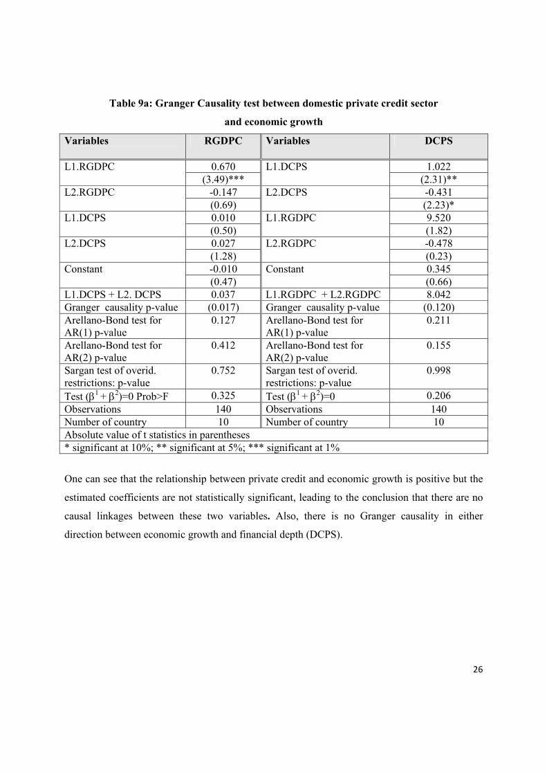
Table 9a: Granger Causality test between domestic private credit sector

and economic growth

Variables

RGDPC Variables DCPS

0.670 1.022 L1.RGDPC (3.49)***

L1.DCPS (2.31)**

-0.147 -0.431 L2.RGDPC (0.69)

L2.DCPS (2.23)*

0.010 9.520 L1.DCPS (0.50)

L1.RGDPC (1.82)

0.027 -0.478 L2.DCPS (1.28)

L2.RGDPC (0.23)

-0.010 0.345 Constant (0.47)

Constant (0.66)

L1.DCPS + L2. DCPS 0.037 L1.RGDPC + L2.RGDPC 8.042 Granger causality p-value (0.017) Granger causality p-value (0.120) Arellano-Bond test for AR(1) p-value

0.127 Arellano-Bond test for AR(1) p-value

0.211

Arellano-Bond test for AR(2) p-value

0.412 Arellano-Bond test for AR(2) p-value

0.155

Sargan test of overid. restrictions: p-value

0.752 Sargan test of overid. restrictions: p-value

0.998

Test (β1 + β2)=0 Prob>F 0.325 Test (β1 + β2)=0 0.206 Observations 140 Observations 140 Number of country 10 Number of country 10 Absolute value of t statistics in parentheses * significant at 10%; ** significant at 5%; *** significant at 1%

One can see that the relationship between private credit and economic growth is positive but the

estimated coefficients are not statistically significant, leading to the conclusion that there are no

causal linkages between these two variables. Also, there is no Granger causality in either

direction between economic growth and financial depth (DCPS).

27 

 

Table 9b: Granger Causality test between interest rate margin

and economic growth

Variables

RGDPC Variables INT

0.646 -0.010 L.RGDPC (8.73)***

L1.INT (0.10)

-0.146 0.274 L2.RGDPC (3.09)**

L2.INT (3.21)**

0.001 7.157 L1.INT (1.96)*

L.RGDPC (1.96)*

-0.003 -17.938 L2.INT (2.17)**

L2.RGDPC (4.29)***

0.019 1.382 Constant (4.90)***

Constant (3.99)***

L1.INT+ L2.INT -0.002 L.RGDPC + L2.RGDPC -10.781 Granger causality p-value (0.035) Granger causality p-value (0.13) Arellano-Bond test for AR(1) p-value

0.151 Arellano-Bond test for AR(1) p-value

0.250

Arellano-Bond test for AR(2)

0.658 Arellano-Bond test for AR(2 p-value)

0.579

Sargan test of overid. restrictions: p-value

0.852 Sargan test of overid. restrictions: p-value

0.901

Test (β1 + β2)=0 0.300 Test (β1 + β2)=0 0.101 Observations 140 Observations 140 Number of country 10 Number of country 10 Absolute value of t statistics in parentheses * significant at 10%; ** significant at 5%; *** significant at 1%

Further, causality runs from banking efficiency (INT) to economic growth but not in the opposite

direction, i.e. the interest rate margin Granger-causes economic growth. This linkage is negative

and significant. Again, there is no evidence of long-run effects of causality from INT to RGDPC

(Prob>F = 0.300 , implying that “H0: no long-run effect” is not rejected).

28 

 

Table 9c: Granger Causality test between stock market capitalisation and economic growth

Variable

RGDPC Variable STMC

0.652 0.373 L1.RGDPC (8.33)***

L1.STMC (2.14)*

-0.092 0.133 L2.RGDPC (1.37)

L2.STMC (1.35)

0.007 -1.206 L1.STMC (3.44)***

L1.RGDPC (0.24)

-0.005 5.439 L2.STMC (2.64)***

L2.RGDPC (2.64)**

0.012 0.494 Constant (5.54)***

Constant (1.94)*

L1.STMC + L2.STMC 0.002 L1.RGDPC + L2.RGDPC 4.233 Granger causality p-value 0.002 Granger causality p-value 0.176 Arellano-Bond test for AR(1) p-value

0.13 Arellano-Bond test for AR(1) p-value

0.151

Arellano-Bond test for AR(2) p-value

0.349 Arellano-Bond test for AR(2) p-value

0.421

Sargan test of overid. restrictions: p-value

0.625 Sargan test of overid. restrictions: p-value

0.836

Test (β1 + β2)=0 Prob>F 0.350 Test (β1 + β2)=0 Prob>F 0.451 Observations 132 Observations 132 Number of country 10 Number of country 10 Absolute value of t statistics in parentheses * significant at 10%; ** significant at 5%; *** significant at 1% Finally, Granger causality runs from stock market capitalisation (STMC) to economic growth

(RGDPC) but not in the opposite direction. There is also no evidence of long-run effects (Prob>F

= 0.350, implying that “H0: no long-run effect” is not rejected).

6. Conclusions In this paper we have reviewed the main features of the banking and financial sector in ten new

EU members, and then investigated the relationship between financial development and

economic growth in these economies by estimating a dynamic panel data model over the period

1994-2007. To summarise, financial depth is found to be lacking in all ten countries, and

therefore the contribution of the relatively underdeveloped credit and stock markets to growth

29 

 

has been rather limited, with only a minor positive effect of some indicators of financial

development. This might be a consequence of the large stock of non-performing loans and the

banking crises experienced by these economies at the beginning of the transition period. In

general, the CEE-5 have more developed financial sectors than the B-3 and SEE-2 countries. By

contrast, the implementation of reforms, the entry of foreign banks and the privatisation of state-

owned banks have reduced transaction costs and increased credit availability. This has improved

the efficiency of the banking sector (Fries et al., 2006), which has played an important role as an

engine of growth. Better regulation and supervision was partly motivated by the European

integration process and the need to adopt EU standards. Thus, many of the banking sector

weaknesses traditionally characterising emerging markets have gradually been eliminated. Given

the prospect of EU accession, foreign banks, mainly from the euro area, seized the opportunity

and established subsidiaries in all CEE countries, seeing them as an extension of the common

European market and becoming dominant players in their banking sectors.

However, the massive presence of foreign banks has also increased contagion risks, and the

consolidation process (with the majority of banks being foreign–owned) could limit competition.

Thus, a financial crisis produced in the mature markets of the euro area could also reach the CEE

countries. A strategy of financial development based on foreign entry from the anchor currency

area is no guarantee for a smooth process of finance and growth, an example being the current

crisis which started in the mature economies in the summer of 2007 and caused a sudden stop of

capital flows to Southeastern Europe (Winkler, 2009).

Granger causality test suggest that causality runs from financial development, measured as credit

to the private sector and the interest rate margin, to economic growth, but not in the opposite

direction. Credit to the private sector has risen rapidly in these countries in recent years but at a

different rate, the lending boom being particularly strong in the segment of loans to households,

primarily mortgage-based housing loans. The heterogeneity in credit dynamics can have various

causes, such as a different degree of economic or financial intermediation development, and

different institutional and regulatory frameworks. Our analysis of the determinants of credit to

the private sector highlights different factors that stimulate credit growth in the transition

30 

 

countries, such as an increase in income or a decrease in lending rates, inflation and non-

performing loans, and the implementation of reforms in the banking sector. Further, the high

growth of credit to households can affect negatively the current account, which might be a

serious problem for the transition economies.

Overall, the underdevelopment of stock and credit markets, with the consequent lack of financial

depth, remains one of the main features of these economies. However, elements of market-

oriented intermediation are now the rule rather than the exception throughout them (Bonin and

Wachtel, 2003), and appropriate policies can reduce financial sector instability that could impair

growth (Kraft, 2005).The adoption of the euro could have a further positive impact on financial

development and economic growth in these countries, but this issue is beyond the scope of the

present paper.

31 

 

References Arellano M., Bond S. (1991), “Some Tests of Specification for Panel Data: Monte Carlo

Evidence and an Application to Employment Equations”, Review of Economic Studies, 58(2),

277-297.

Arellano M., Bover O. (1995), “Another Look at the instrumental variable estimation of error-

components models”, Journal of Econometrics, 68(1), 29-51.

Backé P., Égert B., Walko Z. (2007), “Credit Growth in Central and Eastern Europe Revisited”,

Focus on European Integration 2, 69-77.

Beck T., Levine R., Loayza N. (2000), “Finance and the Sources of Growth”, Journal of

Financial Economics, 58(1-2), 261-300.

Beck T., Feijen E., Ize A., Moizeszowicz F. (2008), “Benchmarking financial development”,

Policy Research Working Paper Series 4638, The World Bank.

Beck T., Demirgüç-Kunt A., Levine R. (2000), “A New Database on the Structure and

Development of the Financial Sector”, World Bank Economic Review 14 (3), 597-605.

Beck T. (2008), “The Econometrics of Finance and Growth”, Policy Research Working Paper

Series 4608, The World Bank.

Bencivenga V.R., Smith B.D. (1991), “Financial Intermediation and Endogenous Growth”,

Review of Economic Studies, 58(2), 195-209.

Berglöf E., Bolton P. (2002), “The Great Divide and Beyond: Financial Architecture in

Transition”, The Journal of Economic Perspectives, 16 (1), 77-100.

Blundell R., Bond S. (1998), “Initial Conditions and Moment Restrictions in Dynamic Panel

Data Models”, Journal of Econometrics, 87(1), 115-143.

Boissay F., Calvo-Gonzalez O., Kozluk T. (2007), “Using Fundamentals to Identify Episodes of

‘Excessive’ Credit Growth in Central and Eastern Europe”, in Enoch C. and I. Ötker-Robe (eds.).

Rapid Credit Growth in Central and Eastern Europe: Endless Boom or Early Warning? 47–66.

Bonin J., Wachtel P. (2003), “Financial Sector Development in Transition Economies: Lessons

from the First Decade”, Financial Markets, Institutions and Instruments 12 (1), 1- 66.

Bonin J., Hasan I., Wachtel P. (2005), “Privatisation Matters: Bank Performance in Transition

Countries”, Journal of Banking and Finance 29, 2153-78.

32 

 

Brzoza-Brzezina M. (2005), “Lending booms in the new EU Member States: will euro adoption

matter”, ECB Working Paper No. 543.

Casu B., Girardone C. (2009), “Testing the relationship between competition and efficiency in

banking: A panel data analysis”, Economics Letters 105 (1), 134–137.

Coricelli F., Masten I. (2004). "Growth and Volatility in Transition Countries: The Role of

Credit," presented at the IMF Conference in honor of Guillermo A. Calvo, Washington, DC,

April 15-16, 2004, International Monetary Fund.

Cottarelli C., Dell’Ariccia G., Vladkova-Hollar I. (2005), “Early Birds, Late Risers and Sleeping

Beauties: Bank Credit Growth to the Private Sector in Central and Eastern Europe and in the

Balkans”, Journal of Banking and Finance, 29(1), 83–104.

De Haas R.T.A (2001), “Financial development and economic growth in transition economies A

survey of the theoretical and empirical literature” Research Series Supervision 35, Netherlands

Central Bank.

Égert B., Backé P., Zumer T. (2007), “Private-Sector Credit in Central and Eastern Europe: New

(Over) Shooting Stars?”, Comparative Economic Studies 49 (2), 201-231.

Fink G., Haiss P., Mantler H.C. (2005), “The Finance-Growth-Nexus: Market Economies vs.

Transition Countries, Europainstitut Working Paper 64.

Fink G., Haiss P., and Vuksic G. (2008), “Contribution of Financial Market Segments at

Different Stages of Development: Transition, Cohesion and Mature Economies Compared”

Journal of Financial Stability, forthcoming.

Fries S., Neven D.J., Seabright P., Taci A. (2006), “Market Entry, Privatization and Bank

Performance in Transition”, Economics of Transition, 14(4), 579-610.

Gillman M., Harris M.N. (2004), “Inflation, Financial Development and Growth in Transition

Countries”, Monash Econometrics and Business Statistics Working Papers 23.

Goldsmith R.W. (1969), “Financial Structure and Development”, New Haven, CT, Yale

University Press.

Granger C.W.J. (1969), “Investigating Causal Relations by Econometric Models and Cross-

Spectral Methods”, Econometrica, 37(3), 424-38.

Granger C.W.J., Lin J. L. (1995),“Causality in the long run”, Econometric Theory, 11 (3), 530-

36.

33 

 

Granger C.W.J. (2003),” Some Aspects of Causal Relationships”, Journal of Econometrics, 112

(1), 69-71.

Greenwood J., Jovanovic B. (1990), “Financial Development, Growth, and the Distribution of

Income”, Journal of Political Economy, University of Chicago Press, 98(5), 1076-1107.

Hagmayr B., Haiss P.R., Sumegi K. (2007), “Financial Sector Development and Economic

Growth - Evidence for Southeastern Europe” EuropaInstitut Working Paper.

Harrison P., Sussman O., Zeira J. (1999), “Finance and growth: Theory and new evidence”,

Finance and Economics Discussion Series 35, The Federal Reserve Board.

Hermes N., Lensink R. (2000), “Financial system development in transition economies” Journal

of Banking and Finance, 24 (4), 507-524.

Im K., Pesaran M.H., Shin Y. (2003), “Testing for unit roots in heterogeneous panels”, Journal

of Econometrics 115 (1), 53-74.

Kenourgios D., Samitas A. (2007).” Financial Development and Economic Growth in a

Transition Economy: Evidence for Poland” Journal of Financial Decision Making, 3, (1), 35-48.

King R.G., Levine R. (1993a), “Finance, Entrepreneurship, and Growth: Theory and evidence”,

Journal of Monetary Economics, 32(3), 513-42.

King R.G., Levine R (1993b), “Finance and Growth: Schumpeter might be right”, Quarterly

Journal of Economics, 108 (3), 717-37.

Kraft E., (2005), “EU Accession - Financial Sector Opportunities and Challenges for Southeast

Europe, Springer Berlin Heidelberg, 61-91.

Levine R. (1997), “Financial development and economic growth: Views and agenda”, Journal of

Economic Literature, 35(2), 688-726.

Levin A., Lin. C.F., Chu C.S., (2002), “Unit root tests in panel data: Asymptotic and finite

sample properties”, Journal of Econometrics, 108(1), 1–24.

Levine R., Zervos S. (1996), “Stock Market Development and Long-Run Growth”, World Bank

Economic Review, 10(2), 323-339.

Levine R., Loayza N., Beck T. (2000), “Financial intermediation and growth: Causality and

causes”, Journal of Monetary Economics, 46(1), 31-77.

34 

 

Levine R. (2005), “Finance and Growth: Theory and Evidence,” Handbook of Economic Growth,

in: Aghion P. and S. Durlauf (ed.), vol 1, 865-934.

Lucas R.E. (1988),“On the mechanics of economic development”, Journal of Monetary

Economics, 22(1), 3-42.

Matousek R., Taci A. (2005), “Efficiency in banking: Empirical Evidence from the Czech

Republic”, Economic Change and Restructuring, 37(3), 225-244.

McKinnon R.I. (1973), “Money and Capital in Economic Development”, Washington D.C., The

Brookings Institution.

Pesaran H.M. (2007), “A simple panel unit root test in the presence of cross-section

dependence”, Journal of Applied Econometrics 22(2), 265-312.

Rioja F., Valev N. (2004), “Does one size fit all? A reexamination of the finance and growth

relationship”, Journal of Development Economics 74(2), 429-47.

Robinson J. (1952), “The generalization of the general theory”, in The Rate of Interest and Other

Essays, London: Macmillan, 69-142.

Rousseau P.L., Wachtel P. (2002), ”Inflation thresholds and the finance-growth nexus”, Journal

of International Money and Finance, 21(6), 777-793.

Schumpeter J.A. (1934), “The Theory of Economic Development”, Cambridge, MA, Harvard

University Press.

Shaw E.S. (1973), “Financial Deepening in Economic Development”, New York: Oxford

University Press.

Tang H., Zoli E., Klytchnikova I. (2000), “Banking Crises in Transition Countries: Fiscal Costs

and Related Issues”, World Bank Policy Research Working Paper 2484.

Wachtel P. (2001), “Growth and Finance: What do we know and how do we know it?”,

International Finance, 4(3), 335-362.

Winter L.A. (2004), “Trade Liberalization and Economic Performance: An Overview,” The

Economic Journal, 114, 4-21

Winkler. A., (2009), “Southeastern Europe: Financial Deepening, Foreign Banks and Sudden

Stops in Capital Flows” Focus on European Economic Integration 1, 84-97.

35 

 

APPENDIX A

Table A1: List of variables

VARIABLE (series)

CODE NOM

Source

BCPS Bank credit to the public sector as a percentage of

GDP

IFS database

DCPS Domestic credit to private sector (in per cent of GDP) EBRD database

GDPC GDP per capita (in PPP) EBRD database

GVE General government expenditure to GDP EBRD database

HC Secondary school enrollment ratio UNESCO database

HCR Domestic credit to households (in per cent of GDP) EBRD database

IBR EBRD index of banking sector reform EBRD database

INFL Inflation, average consumer prices IMF database

INV Investment/GDP (in per cent) EBRD database

INT Interest margin rates between lending and deposit (in

per cent)

Authors’ calculation

using EBRD database

LLG Liquid Liabilities (in per cent of GDP) EBRD database

LR Lending rate (average) EBRD database

NPL Non-performing loans (in per cent of total loans) EBRD database

PCFB Asset share of foreign-owned banks (in per cent) Authors’ calculation

using EBRD database

RGDPC Real GDP per capita growth Authors’ calculation

using EBRD database

RI Reform index of financial institutional development Authors’ calculation

using EBRD database

STMC Stock market capitalisation (in per cent of GDP) EBRD database

TOP Trade openness to GDP EBRD database

36 

 

Table A2. EBRD indicators of reform

Indicator EBRD index of banking sector reform

EBRD index of reform of non-bank financial institutions

Year Country

1996 2007 1996 2007

Bulgaria 2.0 3.7 2.0 2.7 Czech.Rep. 4.3 4.3 2.7 3.0 Estonia 4.0 4.3 2.0 3.7 Hungary 4.3 4.3 3.0 3.3 Latvia 4.0 4.3 2.0 3.0 Lithuania 4.0 4.3 2.0 3.3 Poland 4.3 4.3 2.7 3.3 Romania 3.0 4.3 1.0 2.7 Slovakia 4.3 4.3 3.0 3.3 Slovenia 4.3 4.3 2.0 2.7

Source EBRD

Table A3 : Interest rate margin (%)

Year Country

2000 2001 2002 2003 2004 2005 2006 2007

Bulgaria 8.4 8.2 6.6 5.9 5.8 4.9 4.9 6.3Czech.Rep 3.8 6.1 4.8 4.8 4.8 4.5 4.3 4.6Estonia 2.1 5.6 2.9 2.7 4.1 6.2 3.6 4.1Hungary 2.9 2.6 2.3 2.5 1.9 2.2 1.8 2Latvia 7.7 5.5 2.3 2.4 4 2.7 3.7 4.8Lithuania 9.7 7.4 5.8 4.8 5.4 5.3 5.2 5.3Poland 7.2 8.8 7.4 6.7 7.4 4.2 4.1 4.5Romania 20.8 19.5 16.2 14.4 14.1 13.2 9.2 6.7Slovakia 4.5 5 3.6 3.2 5 4.3 4.1 4.2Slovenia 5.7 5.3 5 4.8 4.9 4.6 4.6 2.3

Source: EBRD

37 

 

Table A4: Mortgage lending (as a percentage of GDP)

Year Country

2000 2001 2002 2003 2004 2005 2006 2007

Bulgaria - - - 1.2 2.7 4.8 7.2 10.4 Czech.Rep 2.0 2.4 3.0 4.2 5.9 7.7 10.0 12.5 Estonia 2.3 3.5 5.5 9.5 14.6 22.6 33.0 37.7 Hungary 1.1 1.7 4.1 8.0 9.5 11.5 13.9 16.4 Latvia 1.6 2.4 4.1 7.6 12.4 19.5 28.9 33.7 Lithuania - - 1.9 3.4 5.5 9.0 12.6 17.2 Poland - - 2.4 3.4 3.8 5.0 7.2 9.9 Romania - - - 0.3 0.5 0.6 0.9 1.4 Slovakia 0.1 0.4 1.0 2.2 2.9 3.6 4.1 4.5 Slovenia 1.7 1.8 2.0 2.3 2.8 4.2 4.5 6.2

Table A5: Levin-Lin-Chu stationarity test

Series Coefficient t-value t-star P > t Level

BCPS -0.54670 -7.485 -4.53383 0.0000 I(0) DCPS -0.24590 -5.356 -2.25883 0.0119 I(0) GDPC -0.15040 -5.358 -3.71969 0.0001 I(0) GVE -0.52960 -7.119 -4.00032 0.0000 I(0) HC -0.25120 -6.727 -4.99531 0.0000 I(0) HCR -0.14939 -3.812 -1.71353 0.0433 I(0) IBR -0.47511 -7.459 -4.42017 0.0000 I(0) INFL -0.46330 -6.384 -2.61235 0.0045 I(0) INT -0.63380 -8.358 -5.17992 0.0000 I(0) INV -0.19084 -3.633 -1.26133 0.0136 I(0) LLG -0.19990 -5.282 -3.15713 0.0008 I(0) LR -0.65490 -8.049 -4.40804 0.0000 I(0) NPL -0.21493 -3.994 -1.29016 0.0985 I(0) PCFB -0.55450 -9.596 -7.97387 0.0000 I(0) RGDPC -0.58719 -8.584 -5.15507 0.0000 I(0) RI -0.43460 -8.835 -5.78175 0.0000 I(0) STMC -0.89160 15.682 -13.67317 0.0000 I(0) TOP -0.28015 -8.240 -6.20488 0.0000 I(0)

38 

 

The Levin-Lin-Chu (LLC) test

The LLC test is based on estimating the following equation:

titiitiiti yty ,1,, ςρθδα ++++=Δ − i = 1,2,…N, t = 1,2,…T

This model allows for two–way fixed effects (α and θ) and unit–specific time trends. Because the

coefficient of the lagged dependent variable is restricted to be homogeneous across all units of

the panel, the unit–specific fixed effects are an important source of heterogeneity. The test

involves the null hypothesis H0 : ρi = 0 for all i against the alternative HA : ρi = ρ < 0, with

auxiliary assumptions about the coefficients of the deterministic components also being required

under the null. The LLC test assumes that the individual processes are cross–sectionally

independent. Given this assumption, conditions (and correction factors) are derived under which

the pooled OLS estimate of ρ will have a standard normal distribution under the null hypothesis.

Levin et al. (2002) analyse the asymptotic distribution of this pooled panel estimate of ρ under

different assumptions on the existence of fixed effects and homogeneous time trends. This test

can be viewed as a pooled Dickey–Fuller (or ADF) test, potentially with differing lag lengths

across the units of the panel.

The Pesaran (2007) test

The Pesaran (2007) test is based on estimating the following equation:

tijtij

jitiiti yyyi

,,1

,1,, εβραρ

+Δ++=Δ −=

− ∑ i = 1,2,…N, t = 1,2,…T

It is essentially a t-test for unit roots in heterogeneous panels with cross-sectional dependence.

Similarly to the Im, Pesaran and Shin (IPS, 2003) test, it is based on the mean of individual DF

(or ADF) t-statistics of each unit in the panel. The null hypothesis is that all series are non-

stationary. To eliminate cross-sectional dependence, the standard DF (or ADF) regressions are

augmented with the cross-sectional averages of lagged levels and first-differences of the

individual series (CADF statistics). This avoids size distortions, especially in the case of models

39 

 

with residual serial correlations and linear trends. When T is fixed, in order to ensure that the

CADF statistics do not depend on the nuisance parameters the effect of the initial cross-sectional

mean must also be eliminated; this can be achieved by applying the test to the deviations of the

variable from the cross-sectional mean. Lags of the dependent variable can be introduced to

control for serial correlation in the errors. The order of augmentation can be estimated using

model selection criteria such as Akaike or Schwartz applied as usual to the underlying time

series specification.

The exact critical values of the t-bar statistic are given by Pesaran (2007). The Z[t-bar] statistic

is distributed standard normal under the null hypothesis of nonstationarity. Pesaran (2007)

suggests that a generalisation of the test to unbalanced panels can be made straightforwardly as

IPS (2003) show. In the case of unbalanced panels only standardised Z[t-bar] statistics can be

computed.