financial flights, stock market linkages and jump excitation

Financial flights, stock market linkages andjump excitation

Mardi Dungeya, Deniz Erdemlioglub,∗, Marius Mateia, Xiye Yangc

aTasmanian School of Business and Economics, University of Tasmania, AustraliabIESEG School of Management and CNRS, France

cDepartment of Economics, Rutgers University, U.S.

This Version: June 24, 2016

Abstract

We propose a new nonparametric test to identify the mutually exciting jumps in high frequency

data. We derive the asymptotic properties of the test statistics and show that the tests behave rea-

sonably well in finite sample cases. Using our mutual excitation tests, we characterize global stock

market linkages and study the dynamics of financial flights. The results suggest that flight-to-safety

episodes (from stocks to gold) occur more frequently than do flight-to-quality cycles (from stocks

to bonds). The excitation channel further appears to be asymmetric at high frequency: emerging

market jumps excite U.S. equities, and the evidence supporting the reverse transmission is quite

weak. The data exhibit a strong excitation effect from volatility jumps to price jumps.

Keywords: Flight-to-safety, Flight-to-quality, Mutual-excitation in jumps, Financial contagion,

Stock-bond comovement, Asset market linkages, Financial crises, High-frequency data, Volatility

feedback effect

JEL: G01, G12, G15, C12, C14, C58

We thank Massimiliano Caporin, Pasquale Della Corte, Ozgur Demirtas, Dobrislav Dobrev, Louis Eeckhoudt,Robert Engle, Neil R. Ericsson, Andrew Harvey, David F. Hendry, Sebastien Laurent, Simone Manganelli, ChristopherJ. Neely, Marc Paolella, Andrew Patton, Olivier Scaillet, Paul Schneider, Victor Todorov, Giovanni Urga, LarsWinkelmann, Kamil Yilmaz and participants at the 9th Annual SoFiE Conference, IAAE 2016 Annual Conference,Federal Reserve Bank of St. Louis Research Seminar and 16th Oxmetrics Financial Econometrics Conference forvaluable comments and helpful suggestions. Dungey and Matei acknowledge funding from Australian ResearchCouncil grant (DP130100168).

∗Corresponding author. IESEG School of Management, 3 Rue de la Digue, Lille, France. Tel: +33 (0)320 545892. Fax: +33 (0)320 574 855.

Email addresses: [email protected] (Mardi Dungey), [email protected] (Deniz Erdemlioglu),[email protected] (Marius Matei), [email protected] (Xiye Yang)

1. Introduction

“U.S. and European stocks dived after a sharp selloff in Chinese shares accelerated,

wiping out gains for the year. Oil prices continued to drop, while Treasurys gained as

investors sought the relative safety of government bonds.”

(Wall Street Journal, August 24, 2015, 3:55 pm−EST)

“This is a flight to quality and the actual level that the Treasury yield achieves in

this environment is not meaningful. This is a time when you dig a deep hole, close your

eyes and put your fingers in your ears.”

(David Keeble, Credit Agricole, Wall Street Journal, August 24, 2015, 4:24 pm−EST)

The global financial system is vulnerable to unforeseen shocks and unexpected events. Sudden

shocks may, for instance, amplify uncertainty, which, in turn, exacerbates fear and increases risk

perception in the marketplace. The downside effects of financial stress could be even worse, espe-

cially when the shocks in one region (or market) spread to others through contagion and market

linkages.1

Over the last two decades, financial markets have experienced various adverse shocks and sudden

crashes. East Asian countries, for instance, were hit by severe financial turmoil during 1997-98,

triggering currency crises and plunges in stock markets in that region. Shortly after the Asian

crisis, the Russian government defaulted on its debt on August 17, 1998, and this event accelerated

the collapse of the hedge fund Long-Term Capital Management (LTCM). Argentina suffered from

a great depression and sharp recession in the beginning of 2000s. More recently, in the United

States, the House voted against the bailout of Lehman Brothers on September 29, 2008. As

Figure 1 displays, the market reaction to this event was rather swift at the intraday level: the S&P

500 index declined sharply around 18:00 GMT, within minutes after the news shock, and the VIX

index—a common proxy for market volatility—elevated substantially.

[ Insert Figure 1 about here ]

How do such historical tail events propagate from one location (or market) to another? What

is the degree of transmission, when does it occur and why do we observe contagion? These ques-

tions are important for the measurement of market risk (embedded in risk spillovers), credit risk

(associated with default spillovers) and systemic/system-wide risk (linked to tail comovements).

For portfolio managers, understanding the linkages of shocks (e.g., between bonds and stocks) is of

1Researchers define the term financial contagion in different ways. Forbes and Rigobon (2002) argue that financialcontagion is an increase in cross-market comovement after a sudden shock to one market (or country). If correlationdoes not increase significantly, it creates only interdependence. Dungey and Martin (2007) separate contagion fromspillover. The difference between two types of linkages is related to the timing of transmission. While contagion refersto a shock transmission occurring contemporaneously between two markets, spillovers arrive with time lags. Dungeyand Martin (2007) further show that spillover effects are larger than contagion effects.

2

interest to evaluate asset allocation and diversification strategies. The risk exposure of portfolios

to sudden global shocks, for instance, depends on the dynamics of linkages. From an option pricing

perspective, derivative analysts consider shock spillovers when valuing derivative securities whose

payoffs typically rely on multiple asset prices.

The literature offers two main directions to study financial contagion. One strand investigates

the sources of shocks that can be linked to information arrivals (Harvey and Huang, 1991, Eder-

ington and Lee, 1993, King and Wadhwani, 1990, Calvo and Mendoza, 2000), liquidity or trading

activity (Diamond, 1983, Caballero and Krishnamurthy, 2008, Jiang et al., 2011, Fleming et al.,

1998). While Dungey et al. (2010), for instance, consider structural shocks as main market crash

drivers, Allen and Gale (2000) exploit the characteristics of real shocks; the innovations to prefer-

ences and consumer behavior in one particular country or asset class.

Another body of research focuses on the measurement of asset market linkages.2 These studies

propose using statistical and econometric methods to analyze financial contagion. For example,

Forbes and Rigobon (2002) investigate the correlation between global stock markets and find rela-

tively weak evidence of contagion.3 Pelletier (2006) extends this work and considers different regime

structures in examining cross correlations. Compared to the multivariate analysis of Evans (2002),

Pelletier (2006) documents smoother correlations across major foreign exchange rates. Chan et al.

(2011) focus on multiple asset classes and show the presence of cross linkages. While Guidolin and

Timmermann (2006, 2007) characterize the nonlinear dynamics of the stock-bond relation, King

and Wadhwani (1990) and, more recently, Diebold and Yilmaz (2014) examine the transmission

of volatility within stock markets.4 These studies suggest that financial volatility exhibits strong

connectedness that varies over time with market conditions.

Despite the substantial progress, relatively little is known about the spillover of abnormal (jump-

type) shocks for several potential reasons. The first reason is broadly linked to a model selection

problem. In practice, the process generating shocks is latent; hence, jumps are not directly observ-

able. This (model uncertainty) problem arises, particularly when researchers seek to exploit the

patterns in high-frequency data. As Aıt-Sahalia and Jacod (2012) point out, tail-type jump events

tend to occur more frequently at short time scales compared to long investment horizons. Therefore,

2The literature on this direction is rather vast. For currency market linkages, see, e.g., Diebold and Nerlove (1989),Mahieu and Schotman (1994), Kaminsky and Reinhart (2000); for stock market linkages, see, e.g., Bae et al. (2003),Forbes and Rigobon (2002), King and Wadhwani (1990), King et al. (1994), Lin et al. (1994), Karolyi (1995), Bekaertet al. (2005), Hamao and Ng (1990), Karolyi and Stulz (1996); and for bond market linkages, see, e.g., Favero andGiavazzi (2002) and Dungey et al. (2000).

3In the literature on asset market linkages, researchers classify contagion in several ways: (i) contagion acrosscountries for a single asset class (e.g., Bae et al., 2003, Karolyi and Stulz, 1996, Karolyi, 1995, Hamao and Ng, 1990),(ii) contagion across different asset classes within a particular region (e.g., Chan et al., 2011), and (iii) contagionacross different countries and asset classes (e.g., Hartmann et al., 2004, Forbes and Chinn, 2004, Dungey and Martin,2007). See also Baur (2012), who studies the effect of financial contagion on the real economy by considering bothdeveloped and emerging stock markets.

4See also Longin and Solnik (1995), Hamao and Ng (1990) and Flood and Rose (2005). Longin and Solnik (1995)is an example of earlier works suggesting time-varying cross-market correlations. Hamao and Ng (1990) and, morerecently, Flood and Rose (2005) analyze the covariance between international stock markets and within the U.S.,respectively.

3

a model that fails to characterize jump linkages at a relatively high frequency might underestimate

the true dependence in shocks. The second challenge is related to the empirical characteristics of

volatility. In financial data, one might notice that the periods of high volatility mingle with the pe-

riods of co-jumps. This is not surprising because sudden crashes might trigger fear and turbulence,

which, in turn, increase market-wise volatility. Such patterns, however, create complications for

the estimation of market risk embedded in jump spillovers and volatility transmission. It is thus

crucial to separate joint jump shocks from volatility linkages. Perhaps more importantly, those

jump-type shocks are likely to propagate over time (e.g., during the crisis), and tail events may

spread with delay. In the presence of such regularities, understanding the origin (or direction) of

jump spillovers may be difficult and ambiguous. Although correlation/covariance-based measures

are certainly of interest in this context, jump-type shock transmission remains elusive.

In this paper, we address these issues and develop a new approach to measure the transmission

of jumps in financial markets. Relying on nonparametric (model-free) testing procedures, this

approach allows us to characterize the dynamic properties of shock transmission in greater depth

than is possible with correlation/covariance analysis or traditional co-jump techniques. In our

continuous-time setup, jump-type shocks in one financial asset (or region) have the potential to

cluster over time and to increase the intensity of jumps in other assets (mutual excitation). We

derive the asymptotic behavior of these mutual excitation tests and assess their finite sample

performance via simulations. Applying the tests to high-frequency data, we study episodes of

financial flights (i.e., risk-on-risk-off trades), measure directional stock market linkages and examine

the link between jumps in volatility and jumps in asset prices.

Our paper makes three contributions to the extant literature. First, we propose a new non-

parametric test for identifying common jump arrivals in high-frequency data. Our econometric

procedure is particularly related to the multivariate tests of Bollerslev et al. (2008), Jacod and

Todorov (2009), Mancini and Gobbi (2012) and Bibinger and Winkelmann (2015). Among these

studies, Bollerslev et al. (2008) identify cojumps by utilizing cross-covariance of asset returns. Ja-

cod and Todorov (2009) extend the test of Bollerslev et al. (2008) to a generalized framework based

on two possible hypotheses (common jumps or disjoint jumps). The study by Mancini and Gobbi

(2012) is the first to develop the formal truncation method to pin down cojumps. Building on

Jacod and Todorov (2009) and Mancini and Gobbi (2012), the cojump analysis of Bibinger and

Winkelmann (2015) accounts for non-synchronous trading and market microstructure noise in the

data. Perhaps surprisingly, these studies consider jumps as Levy-type (i.e., either Poisson or pure

Levy), and hence, cojumps occur randomly (in theory) with no memory.5 Moreover, the statistical

problem is typically assumed to be symmetric in the literature, that is, jumps arrive simultane-

ously and the origins of shocks may be negligible. We relax these assumptions and minimize these

5Empirically, several studies link cojumps to news announcements. For example, Lahaye et al. (2011) considervarious asset classes and find evidence that macro news creates cojumps. Dungey and Hvozdyk (2012) focus on theU.S. Treasury bond market and study cojumps between spot prices and futures. Bibinger et al. (2015) use ECBmonetary policy surprises to explain cojump patterns in interest rates.

4

restrictions on jump dynamics. In a rather tractable specification, we allow the jumps in one asset

to increase the jump intensity of the other asset, not necessarily contemporaneously but with lags.

Cojumps are directional events in our identification. For instance, while the jumps in asset A

excite the shock occurrences in asset B, the reverse directional effect may not hold in practice (i.e.,

from B to A). As we shall discuss later, we propose four different tests for the four possible null

hypotheses (absence of jump excitation from A to B, or B to A; presence of jump excitation from

A to B, or B to A). We develop the concept, derive the asymptotic properties of the test statistics

and show that the tests behave reasonably well in finite sample cases.


Second, we study the dynamics of financial flights associated with mutually exciting jump-type

tail events. Researchers often define flights as periods of risk-off trades, when market participants

flee relatively risky investments (such as stocks) and invest in safe assets (i.e., flight to safety

(FTS)) or assets of high quality (i.e., flight to quality (FTQ)). As widely reported in the media,

these episodes typically occur when market conditions abruptly deteriorate due to certain political

or news events.6 Figure 2 illustrates an example of an intraday financial flight that occurred on

August 5-6, 2014, when the tension in the Middle Eastern and Ukraine-Russia conflicts increased

significantly. In the figure, the Bloomberg trading screen exhibits a sharp sudden decline in the

index—around 19:30 GMT—as gold prices surged rapidly. Studying financial flights is of interest

not only in terms of understanding the behavior of investors but also in terms of measuring risk

transmission (and premia) within the global financial system. Recent academic research has focused

on the identification and determinants of these events. For instance, Caballero and Krishnamurthy

(2008) develop a theoretical model and show that unusual and unexpected events lead to FTQ

trades. Baele et al. (2014) confirm this view empirically by identifying international FTS. In this

direction, Goyenko and Sarkissian (2015) consider U.S. macroeconomic shocks to be drivers of

FTQ. Engle et al. (2012) focus on the market microstructure and examine the dynamics of the

U.S. Treasury market around FTS periods.7 Unlike Baele et al. (2014) and Goyenko and Sarkissian

(2015), we characterize financial flights at the intraday level. High-frequency data allow us to more

precisely measure the arrivals (and magnitudes) of large adverse shocks in assets. While Longstaff

(2004) and Engle et al. (2012) focus on the U.S. Treasury market, we examine not only bonds

but also stocks and commodities. Compared to these studies, the identification approach in this

6For instance, Bloomberg reported the following headline on July 10, 2014 at 4:03 pm−EST. “Stocks from U.S. toEurope slid as increasing concern over signs of financial stress in Portugal sent investors seeking safety in Treasuries,the yen and gold.”

7In this paper, we restrict our attention to the dynamics of FTS and FTQ. It is worth noting that financialflights could also come in other forms, such as flight to liquidity (FTL) trades. In this alternative direction, Vayanos(2004) develops an equilibrium model and shows that risk aversion increases during periods of turmoil, and investorsexperience a sudden and strong preference for holding bonds. Liquidity premium is time-varying and increases withvolatility. Extending this approach, Brunnermeier and Pedersen (2009) theoretically link market liquidity to FTQ.Beber et al. (2009) analyze European bond market and provide evidence that investors demand credit liquidity—rather than quality—in times of crisis: FTL dominates FTQ. From an empirical perspective, Longstaff (2004) studiesthe risk premium implications of FTL in the U.S. Treasury bond market.

5

paper is non-parametric and flexible enough to capture the different strengths of shocks and time

variation in FTS/FTQ regimes. Our empirical analysis reveals that FTS periods (from stocks to

gold) occur more frequently than FTQ cycles (from stocks to bonds). Interestingly, however, as

adverse shocks become severe, the activity of financial flights decreases substantially. In addition,

we explore seeking returns strategies (SRS) used by investors when risk appetite increases in the

marketplace. We find evidence of such SRS patterns in the data. The results suggest that SRS

episodes exhibit asymmetry, likely reflecting the fact that as market conditions improve, traders

prefer to sell gold, rather than bonds, to invest in stocks.

The third contribution of the paper is the analysis of the stock-bond relationship and asset

market linkages. In the stock-bond literature, our paper is particularly related to the studies

by Panchenko and Wu (2009), Baele et al. (2010) and Bansal et al. (2014).8 Panchenko and Wu

(2009) link stock-bond comovements to emerging market integration.9 Estimating a dynamic factor

model with quarterly data, Baele et al. (2010) show that the drivers of stock-bond comovements are

mostly liquidity and uncertainty factors, and the role of fundamental/macro information is quite

weak. Bansal et al. (2014) conclude that negative stock-bond correlations are due to stronger link

between risk and returns. Our empirical analysis is based on high-frequency data, and we examine

the stock-bond relationship associated with jump-type tail events rather than correlations. Like

Bae et al. (2003), we consider the possibility that severe shocks may propagate differently from

small shocks. However, while Bae et al. (2003) utilize extreme value theory based on low-frequency

return distribution, we adopt a nonparametric approach relying on continuous time. Our sample

is larger and more recent than that used by Bae et al. (2003). Investigating global stock market

integration, we provide evidence that the linkages between developed and emerging stock markets

are considerably asymmetric. In particular, we find that jump-type events hitting Latin American

stocks tend to excite U.S. stocks and that evidence supporting reverse transmission is rather weak.

This result confirms the view of Bae et al. (2003) but contradicts the conclusions by Aıt-Sahalia et al.

(2014). The trading frequency—short or long—thus becomes crucial in identifying the direction of

cross-border spillover effects.

This paper is even more closely related to the studies that empirically analyze linkages during

crisis periods and financial turmoil (e.g., Hartmann et al., 2004, Dungey and Martin, 2007 and

Glick and Hutchison, 2013). Glick and Hutchison (2013) document strong stock market linkages

between China and Asia around the 2008-2009 crisis. Hartmann et al. (2004) estimate the tail

dependence between stock and bond markets of G-5 countries. The analysis by Hartmann et al.

(2004) is based on weekly data over the 1987-1999 period (i.e., around 663 weekly returns). Our

approach, however, focuses relatively more on recent market conditions (2007-2013) and detects

8For other specifications to test for market linkages and stock-bond comovements, see, e.g., Andersen et al. (2007),Forbes and Rigobon (2002), Hartmann et al. (2004), Chordia et al. (2005), Connolly et al. (2005), Kim et al. (2006)and Karolyi and Stulz (1996).

9For other studies analyzing emerging market integration, see, e.g., Bekaert and Harvey (1995, 1997, 2000) andDe Jong and De Roon (2005).

6

linkages from intraday data (i.e., around 141,000 5-minute returns). To identify tail spillovers,

Hartmann et al. (2004) calculate the expected number of crashes given other market crashes. The

testing procedure by Hartmann et al. (2004) is thus ex ante, whereas we utilize ex post realized

measures in continuous time, such as integrated volatility and threshold power variation. We find

evidence of cross-excitation in jump tails between (i) U.S. stocks and U.S. bonds, (ii) U.S. stocks

and emerging market stocks, and (iii) market volatility and asset prices. Our results suggest that

stock market linkages are relatively strong in times of turbulent periods, such as the liquidity case

of BNP Paribas, the bankruptcy of Lehman Brothers, the rescue of AIG, the implementation of

the Trouble Assets Relief Program, and the intensification of the European debt crisis (2011-2012).

The theoretical contribution of this paper builds directly on Boswijk et al. (2014). Our bivariate

(mutual excitation) analysis extends the univariate (self-excitation) approach of Boswijk et al.

(2014). Further, we show that the asymptotic behavior of the test statistics remain fairly similar

to that of self-excitation tests. Boswijk et al. (2014) measure self-excitation in jumps of a single

asset. In contrast, we are interested in testing for mutual excitation in jumps between (at least) two

assets. Therefore, our approach identifies the jump propagation in space, whereas Boswijk et al.

(2014) examine jump propagation in time.

Our paper extends Aıt-Sahalia et al. (2014) and Aıt-Sahalia et al. (2014b) in several respects. In

contrast to the parametric model specifications of these studies, our approach is nonparametric and

relies on test statistics that are model-free. This feature allows us to be flexible in characterizing

the (bivariate) log-price process: the coefficients of the diffusion terms, volatility components, jump

sizes, and jump intensity process can be in any (semimartingale) form. We derive the asymptotic

behavior (level and power) of the test statistics and consider different null hypotheses to identify

the periods of mutual excitation in the data.

Aıt-Sahalia et al. (2014) and Aıt-Sahalia et al. (2014b) consider a finite jump activity for the

underlying Hawkes-type return variation. We relax this assumption in our methodological setup:

jumps can exhibit infinite activity with mutual excitation. We can thus generalize the dynamics of

jump-type financial shocks in a rather comprehensive way. Shocks can be large (and rare) or small

(and frequent). Furthermore, we vary the jump size (i.e., the excitation threshold) and, hence,

capture different levels of jump propagation in the form of weak, mild or severe transmissions.

On the methodological side, our model setup is based entirely on continuous-time. Unlike

Aıt-Sahalia et al. (2014) and Aıt-Sahalia et al. (2014b), we rely on intraday data—rather than

daily data—to test for cross-excitation across assets. The use of high-frequency data gives us more

accurate information about the realized return characteristics, latent (spot) market volatility and

jump dynamics. On the empirical front, Aıt-Sahalia et al. (2014) and Aıt-Sahalia et al. (2014b)

study mutual excitation in international stock markets and European sovereign CDS, respectively.

Instead, our focus is the excitation channel between U.S. and emerging stock indices, commodities

and long-term debt securities. We identify FTS and FTQ fund flows in financial markets using our

mutual excitation tests. Implementing this approach, we further provide evidence of leverage and

volatility feedback effects associated with jumps and excitations.

7

The remainder of this paper is organized as follows. Section 2 introduces the formal setup, the

base methodology and testing procedures. In Section 3, we present the Monte Carlo simulations

to assess the finite sample performance of the tests. Section 4 describes the data and reports our

empirical results. We check the robustness of our results in Section 5. Section 6 concludes.

2. Methodology

2.1. Excitation dynamics of jump-type shocks

Our objective is to identify the transmission of large shocks from one asset (or region) to another.

Before introducing our formal setup, we first illustrate the excitation dynamics as in Aıt-Sahalia

et al. (2014) and Aıt-Sahalia et al. (2014b). Consider two assets (d = 1, 2) and let the log-price of

each asset follow a semimartingale Ito:

dXd,t = µd,tdt+ σd,tdWd,t + ξd,tdNd,t, d = 1, 2, (1)

with a Hawkes-type jump intensity process

dλd,t = αd(λd,∞ − λd,t)dt+2∑

l=1

βd,ldNl,t, d, l = 1, 2, (2)

where µd,t is the drift term, σd,t is the stochastic volatility component, and Wd,t denotes a standard

Brownian motion. In (1), ξd,t denotes the jump size at time t and Nd,t is a Hawkes process for each

asset d = 1, 2. The intensity of jumps follows the dynamics in (2) with conditions αd > βd,l > 0

and λd,∞ > 0 for d, l = 1, 2.10 For ease of exposition, we can rewrite (2) as

λ1,t = λ1,∞ +

∫ t

−∞β1,1e

−α1(t−s)dN1,s +

∫ t

−∞β1,2e

−α1(t−s)dN2,s, (3)

λ2,t = λ2,∞ +

∫ t

−∞β2,1e

−α2(t−s)dN1,s +

∫ t

−∞β2,2e

−α2(t−s)dN2,s, (4)

where λ1,t and λ2,t are the shock intensity processes of assets 1 and 2, respectively. The intuition

behind the setup in (3)−(4) is the following. Consider the jump dynamics of asset 1 (i.e., Equation

(3)). Whenever a sudden shock (dN2,s = 1) occurs in asset 2, λ1,t jumps with magnitude β1,2. The

jump intensity λ1,t then mean-reverts back towards λ1,∞ at speed α1. This specification delivers

two types of feedback mechanism. First, the jump intensity of each asset changes over time and

responds to past jumps (via β1,1 and β2,2). This is the self-excitation of jumps. Second, jump

events in one asset propagate across markets and increase the chance of future shocks in other

assets (via β1,2 and β2,1). The latter effect is the mutual excitation that we wish to capture. The

next section now introduces our modeling framework.

10These conditions ensure that intensities of shocks follow stationary Markov processes.

8

2.2. The model setup

Throughout, we fix a probability space (Ω, Ft, P) where Ω is the set of events in financial

markets, Ft : t ∈ [0, T ] is (right-continuous) information filtration for investors, and P is a data-

generating measure. We follow Boswijk et al. (2014) and consider the Grigelionis decomposition of

Xd,t in (1). That is,

Xd,t = Xd,0 +

∫ t

0bd,sds+

∫ t

0σd,sdWd,s + xd ∗ (µd,t − νd,t) + (xd − h(xd)) ∗ µd,t, (5)

where bd = (bd,t) and σd = (σd,t) are locally bounded, µd is the jump measure of Xd and νd is its

jump compensator that adopts the following decomposition

νd(dt, dx) = dt⊗ Fd,t(dx).

We further assume that the predictable random measure Fd,t can be factored into two parts:

Fd,t(dx) = fd,t(x)λd,t− dx. (6)

Here, the predictable function fd,t(x) controls the jump size distribution and λd,− = (λd,t−)11 is

the stochastic jump intensity or stochastic scale, where

λd,t = λd,0 +

∫ t

0b′d,sds+

∫ t

0σ′d,sdWd,s +

∫ t

0σ′′d,sdBd,s + δd,1 ∗ µ1,t + δd,2 ∗ µ2,t + δ′′ ∗ µ⊥

d,t, (7)

where B is a standard Brownian motion independent of W , µ⊥d is orthogonal to µ1 and µ2, and δd,1,

δd,2, δ′′d are predictable. Boswijk et al. (2014) identify self-excitation through the common jumps

between a log price process X and its own jump intensity λ.12 We extend their framework to test

for mutual excitation in jumps across assets. Consider a function of, for example, X1 and λ2 as

follows.

U(H)t =∑

0≤s≤t

H(X1,s−, X1,s+, λ2,s−, λ2,s+). (8)

The idea is then to choose a function H for R×R×R∗+ ×R

∗+ such that U(H)T behaves distinctly

when X1 and λ2 (the jump intensity of X2) do or do not co-jump within the interval [0, T ]. For

instance, one may choose a function H such that

H(x1, x2, y1, y2) = 0 ⇐⇒ x1 = x2 or y1 = y2, (9)

11For each t > 0, λd,t− := lims↑t λd,t. Similarly, λd,t+ := lims↓t λd,t.12See Aıt-Sahalia and Hurd (2016) for an alternative model of optimal portfolio selection when jumps are mutually

exciting. While Li et al. (2016, 2014) use jump regressions to identify jump size dependence (based on constantintensity), we focus on the interaction between jumps and time-varying jump intensity process. In this direction,Corradi et al. (2014) propose a self-excitement test for constant jump intensity in asset returns.

9

or

H(x1, x2, y1, y2) 6= 0 ⇐⇒ x1 6= x2 and y1 < y2, (10)

or even more specifically, one can consider

H(x1, x2, y1, y2)

> 0 if x1 6= x2 and y1 < y2,

= 0 if x1 = x2 or y1 = y2,

< 0 if x1 6= x2 and y1 > y2.

(11)

Remark 1. If at a time point t, we have |∆X1,t| = 0, then no matter which above condition H

satisfies, the value of H at this time point is zero. If |∆X1,t| 6= 0, then H will take different values

according to whether ∆λ2t is equal to, greater than, or smaller than zero. We summarize the sign

of H for each case in Table 1.13

[ Insert Table 3 about here ]

Remark 2. A complication may arise when |∆X1,t|∆λ2,t > 0 and |∆X2,t| 6= 0. That is, the

positive jump in λ2,t may come from the jump in X1,t, X2,t or both. In this case, it is not possible

to disentangle the effect of X1,t and that of X2,t. However, many common jumps indicate that

other driving forces might trigger these common jumps.14

One challenge here is that the jump intensity process is not observable. To determine the value

of H at each jump time of X1, we need to estimate the spot values of λ2 before and after this jump

time. To achieve this goal and define mutual excitation in jump-type shocks, we make the following

assumption for Fd,t (in (6)).

Assumption 1. Suppose the drift and volatility processes bd,t and σd,t (d = 1, 2) are locallybounded. Assume that there are three (nonrandom) numbers βd ∈ (0, 2), β′

d ∈ [0, βd) and γ > 0,and a locally bounded process Lt ≥ 1, such that, for all (ω, t),

Fd,t = F ′d,t + F ′′

d,t, (12)

where

(a) F ′d,t(dx) = fd,t(x)λd,t−dx with λ = (λd,t) given by (7), λd,t ≤ Lt and

fd,t(x) =1 + |x|γhd(t, x)

|x|1+β, (13)

13In practice, we believe that it is quite unlikely to have ∆λ2t < 0 when |∆X1,t| 6= 0. In other words, the likelihoodthat a jump in X1 will decrease the intensity of X2 is very small because price jumps rarely stabilize financial marketconditions.

14It is worth noting that we are not making causal inferences here. We are particularly interested in tracing whetheror not the jumps in X1 will be accompanied by a positive jump in the intensity of X2.

10

for some predictable function hd(t, x), satisfying

1 + |x|γhd(t, x) ≥ 0, |hd(t, x)| ≤ Lt. (14)

(b) F ′′d,t is a measure that is singular with respect to F ′

t and satisfies

∫

R

(|x|β′ ∧ 1)F ′′d,t(dx) ≤ Lt. (15)

Given these dynamics, we assume that the log-price process Xd,t in (1) is observed at discrete

points in time. For each asset (d = 1, 2), the continuously compounded i-th intraday return of

a trading day t is given by rt,i ≡ X(t+i∆n) − X(t+(i−1)∆n), with i = 1, ...,M and trading days

t = 1, ..., T . Let M ≡ ⌊1/∆n⌋ denote the number of intraday observations in one day. ∆n = 1/M

is then the time between consecutive observations, the inverse of the observation frequency. To

characterize mutual excitation, we introduce a testing procedure that relies on certain functional

forms and jump intensity estimators. Extending the methodological framework of Boswijk et al.

(2014), we begin by defining these measures.

Definition 1. For each asset d = 1, 2, let U(H)t denote the functional of Xt in (1). The estimatorof U(H)t is then given by

U(H, kn)12t =

[t/∆n]−kn∑

i=kn+1

H(X1,i−1, X1,i, λ(kn)2,i−, λ(kn)2,i)1|∆ni X1|>α∆

n , (16)

where kn is an integer and α∆n is the truncation threshold indexed by α (> 0) for a constant

(0 < < 1/2).

In the functional form (16), λ(kn) is the estimator of the (spot) jump intensity λt given by

λ(kn)2,i =∆β2

n

kn∆n

i+kn∑

j=i+1

g

( |∆njX2|

α∆n

)αβ2

Cβ2(1), (17)

where β ∈ (0, 2] is the jump activity index and kn satisfies (1/K ≤ kn∆ρn ≤ K) for (0 < ρ < 1)

and (0 < K < ∞). In (17), g(·) is an auxiliary function that disentangles jumps from the diffusion

component. As in Jing et al. (2012), we assume that this function g(·) satisfies

g(x) =

|x|p if |x| ≤ 1,

1 if |x| > 1,

for an even integer p > 2 and (x := |∆njX|/α∆

n ). For the intensity estimator (17), the quantity

Cβ(1) = 1 for g = 1x>1 and its general form can be given by

Cβ2(kn) =

∫ ∞

0(g(x))kn/x

1+β2dx.

11

In sum, the estimates for the functional form U(H) and jump intensity λt allow us to construct

a test statistic to identify the mutual excitation across financial assets. This implies that we first

need to estimate the spot jump intensities (via Equation (17)) and then use the estimates for

calculating the measure in Equation (16). Armed with this setup, we present the main hypotheses

and the corresponding testing procedures in the next section.

2.3. Hypotheses and testing procedures

Our identification approach for market linkages relies on mutual excitation dynamics. To char-

acterize financial flights and market shock dependence, the first step is to test for the presence of

cross-excitation in jumps. Let X1 and X2 denote asset 1 and asset 2, respectively. Empirically,

we ask the following question: do jumps in asset X1 (X2) excite the jump occurrences in asset X2

(X1)? To answer this question, we consider the following testable hypotheses:

(A) H0: No jump excitation from X1 to X2 vs. H1: Jump excitation from X1 to X2

(B) H0: No jump excitation from X2 to X1 vs. H1: Jump excitation from X2 to X1

(C) H0: Jump excitation from X1 to X2 vs. H1: No jump excitation from X1 to X2

(D) H0: Jump excitation from X2 to X1 vs. H1: No jump excitation from X2 to X1

These hypotheses allow us to investigate not only the jump cascades across regions but also the

origins of shocks. To proceed, let ω denote a specific outcome, i.e., ω ∈ Ω. Methodologically, we

need to make an inference about ω, given a discretely observed sample path over [0, T ]. The outcome

could belong to the “no excitation set” (ω ∈ ΩnoT ) or to the “excitation set” (ω ∈ Ωmut

T ). We test

(A)−(D) by comparing a test statistic to its probability limit under the alternative hypotheses.

We first consider the null hypotheses of “no mutual excitation” (i.e., (A) and (B)).

Theorem 1. Let ∈ (0, 1/2). Suppose that Assumptions 1, 2, 3 (see Appendix A) hold withp > 1−β2

1/2− , q ≥ 2 and q′ ≥ 1, and

1−β2 < ρ < (1−β2) + 2φ′ ∧ 2φ′′ ∧ 1

2β2, (18)

In addition, if either one of the following conditions is satisfied,

(a) H(x1, x2, y1, y2) = 0 for |x1 − x2| ≤ ǫ, where ǫ > 0;

(b) q′ > 2, 2β1 < 1 and ρ < 1−β2 + 2((q′/2− 1) ∧(q ∧ q′ − β1)

).

then, for any fixed t > 0, under H0 of (A), we have

t12n :=

√kn∆n

∆βn

U(H, kn)12T√

U(G, kn)12T

Lst.−−→ N (0, 1), (19)

where U(G, kn)T is the consistent estimator of the conditional variance with

G(x1, x2, y1, y2) =αβCβ(2)

(Cβ(1))2(y1H

′3(x1, x2, y1, y2)

2 + y2H′4(x1, x2, y1, y2)

2), (20)

12

where H ′3 and H ′

4 stand for the first partial derivatives of the function H(.) with respect to its 3rdand 4th arguments, respectively. H(.) can be in the following form:

H(x1, x2, y1, y2) = |x2 − x1|p(2 · log

(y1 + y2

2

)− log(y1)− log(y2)

). (21)

However, under H1 of (A), we have |t12n | P−→ ∞.Therefore, the following critical region has an asymptotic level α for testing the null hypothesis

of “no mutual excitation” (i.e. Ωno

T ), and asymptotic power 1 for the alternative (i.e., Ωmut

T ):

Cno

n =t12n > zα

, (22)

where P(W > zα) = α and W is a standard normal random variable.

Under the null hypothesis of “mutual excitation” (i.e., (C) and (D)), the asymptotic behavior

of the test statistic is as follows.

Theorem 2. Assume P (Ω(−)T ) = 0 and that the same assumptions as in Theorem 1 hold, but with

(H-1) replaced by (H-2). In addition, assume H satisfies the following degenerate condition:

y1 = y2 =⇒ ‖H ′3(x1, x2, y1, y2)‖+ ‖H ′

4(x1, x2, y1, y2)‖ = 0. (23)

If either condition (a) or (b) in Theorem 1 is satisfied, then the following critical region has anasymptotic level α for testing the null hypothesis Ωmut

T :

Cmut

n = |Rn| > zα√Vn, (24)

where

Rn =U(H,wkn)T − U(H, kn)T

U(H, kn)Tand Vn =

∆βn

kn∆n

(w − 1)U(G, kn)Tw(U(H, kn)T )2

. (25)

Moreover, choose a sequence of positive numbers vn such that

vn → 0, andknvn∆n

∆βn

→ ∞,

and set V ′n = Vn ∧ vn. Then, the critical region

C ′mut

n = |Rn| > zα√V ′n (26)

has an asymptotic level α for testing the null hypothesis Ωmut

T and asymptotic power 1 for the

alternative Ω(0)T .

Therefore, we have two statistics to test for mutual excitation between jumps. Under the null

hypothesis of no mutual excitation (i.e., (A) and (B)), we have the statistic in (19), and under the

null hypothesis of excitation (i.e., (C) and (D)), we use the statistic in (26).

13

3. Monte Carlo study

Having presented our testing procedures and hypotheses, we now assess the finite sample prop-

erties of the test statistics. Throughout this section, we consider an observation length of one

week and a sampling frequency of 5 seconds. We thus set T = 5/252 and M = 23400, giving

∆n = 1/23400. Following Aıt-Sahalia and Jacod (2009) and Jing et al. (2012), we further choose

the values = 1/3, ρ = 0.6 and β = 1.25. We conduct each simulation with 1000 replications.

3.1. Simulation setup

Our simulation setup is based on a bivariate Hawkes process with mutually exciting jumps. As

in Aıt-Sahalia et al. (2014) and Boswijk et al. (2014), we consider the following data-generating

process:

dX1,t = σ1,tdW1,t + λ2,∞dY1,t

dX2,t = σ2,tdW2,t + λ2,t−dY2,t

dσ21,t = dσ2

2,t = κ(θ1 − σ21,t) + η1σ1,tdB1,t

dλ2,t = κλ(λ2,∞ − λ2,t)dt+ ηλdB′2,t + ξ 1|∆X1,t|>ǫ.

where the Brownian motions (W1,t, W2,t, B1,t, B′2,t), and the β-stable jump processes (Y1,t, Y2,t)

are assumed to be independent. We consider E [dW1,tdBt] = φdt, which allows us to capture a

potential leverage effect between prices and volatility dynamics. For the volatility process (third

equation), we follow Jing et al. (2012) and set κ = 5, θ1 = 1/16, η1 = 0.5 and φ = −0.5. For

the jump intensity process (fourth equation), we set κλ = 1400, ηλ = 200 and ǫ = 100√θ∆

n as in

Boswijk et al. (2014). λ2,∞ further denotes the constant jump intensity, and we calibrate this value

to generate pre-specified values of the tail probability for 0.25%. That is,

P (|λ2,∞∆ni Y1| ≥ α∆

n ) ≈2cβλ

β2,∞∆n

β(α∆n )

β, (27)

where

cβ =Γ(β + 1)

2πsin

(πβ

2

). (28)

We set α = 5√θ, and β denotes the jump activity index. With the choice of β = 1.25, the calibrated

value for λ∞ is approximately 20.15

The intuition behind our simulation setup is the following. When we set ξ = 0, there is no

mutual excitation in jumps from one asset (X1) to another (X2). In this case, we can thus consider

(i) a null hypothesis of no mutual excitation (i.e., (A)) or (ii) a null hypothesis of mutual excitation

(i.e., (C)). For each null, we can check the size and power of the testing procedures. Similarly,

15In Section 5, we check the sensitivity of the test statistics to different β values. The results for β = 1.5 andβ = 1.75 are rather similar.

14

when we set ξ > 0, jumps can excite as long as the price changes are large enough (i.e., when

|∆nX1,t| > ǫ). To choose the excitation parameter ξ, we utilize the following form

P (|(λ2,∞ + ξ)∆ni Y1| ≥ α∆

n )

P (|λ2,∞∆ni Y1| ≥ α∆

n )≈

(λ∞ + ξ

λ∞

)β

= (1 + ξ/λ∞)β . (29)

For ξ = 12, the ratio in (29) is around 1.80. This implies that the mutual excitation effect will

increase the tail probability by 80% (in relative terms), which is statistically and economically

significant. Given this setup, the test statistic is given by

T :=

√kn∆n

∆βn

U(H, kn)T√U(G, kn)T

P−→ −∞ ω ∈ Ω(−)T ,

−→N (0, 1) ω ∈ Ω(0)T ,

P−→ +∞ ω ∈ Ω(+)T ,

where the function H takes the following form

H(p, q) = H(x1, x2, y1, y2; p, q) = |x2 − x1|p · (y2 − y1)q · 1|x2−x1|≥ǫ, (30)

where ǫ > 0 and—following Boswijk et al. (2014)—we consider two alternative functions for H(p, q):

H(6, 1) and H(0, 1). The next section reports the finite sample properties of our testing procedures.

3.2. Simulation results

To check the power and size properties, we consider four null hypotheses—presented in Sec-

tion 2.3 ((A) to (D)). We proceed as follows. In the next section, we set the excitation parameter

ξ = 0 in order to test for no mutual excitation in all directions, that is, either from X1 to X2 or

from X1 to X2. In Section 3.2.2, we conduct simulations when ξ = 12 and test for the mutual

excitation in jumps. In the final section, we adjust our simulation setup to test specifically for the

financial flights from one asset to another.

3.2.1. Size and power properties: testing for no mutual excitation

We start by considering the null hypothesis (A) such that jumps in asset X1 do not excite

the jumps in asset X2. Figure 3 shows the size and power of the tests for no mutual excitation

in jumps. The solid line in the upper-left panel of the figure indicates that the size of the test is

rather good. That is, when ξ = 0 (no excitation), the percentages of rejection, (i.e., T > zα), are

all close to their corresponding nominal level, α.


In a similar way, we further analyze the size of the test under the null hypothesis that X2 jumps

do not excite X1 jumps (hypothesis (B)). The upper-right panel of Figure 3 shows that the test

also exhibits a well-behaved size in this direction of jump transmission. The Monte Carlo rejections

are close to the nominal level of the test at a 5-second sampling frequency.

15

We can examine the power of the test by considering the same excitation parameter ξ = 0.

Intuitively, if there is no mutual excitation in jumps (i.e., ξ = 0), we should reject the null hypotheses

of mutual excitations (corresponding to hypotheses (C) and (D)). The dotted (dashed-dotted) line

in the upper-left (-right) panel of Figure 3 displays the power performance. Two results emerge from

the panels. First, under the null hypothesis that jumps in X1 excite the jumps in X2 (hypothesis

(C)), the power of the test is weak (dotted line). Second, if we consider a null hypothesis of (reverse)

mutual excitation from X2 to X1 ((hypothesis (D)), then the test has good power (dashed-dotted

line). This implies that—in the absence of mutual jump excitation in the data (i.e., ξ = 0)—we

reject the null hypothesis of mutual excitation from X2 to X1.

3.2.2. Size and power properties: testing for mutual excitation

We now assess the size and power of our tests in the presence of mutual excitation between

jumps. We set the excitation parameter as ξ = 12, which is a reasonable value implying that

mutual excitation (originated in asset X1) will increase the tail event likelihood (in X2) by 80%.

Figure 4 displays the size and power of the tests for mutual excitation in jumps.


The upper-left panel of Figure 4 (dotted line) shows that the test has good size under the null

hypothesis that jumps in X1 excite the jumps in X2 (i.e., hypothesis (C)). Put differently, if there

are jumps in the data, we do not reject the null hypothesis of jump excitation from X1 to X2. The

percentages of rejection in simulations are close to the corresponding nominal level α.

The upper-left panel of Figure 4 (solid-line) further indicates that the power of our test is quite

reasonable. That is, in the presence of mutual excitation, if we consider the null hypothesis that

there is no mutual excitation from X1 to X2 (hypothesis (A)), we reject this null hypothesis in

simulations.

With the choice of ξ = 12 (presence of mutual excitation), we plot in Figure 4 (upper-right

panel) the size and power performance of our test. We now consider the null hypothesis that jumps

in X2 do not excite the jumps in X1 (hypothesis (B)). The percentages of rejection in the figure

depict a forty-five-degree (dashed) line, indicating a well-behaved size. This result is consistent

with the size performance when the null hypothesis is an excitation from X1 to X2. In other words,

if there is an excitation from X1 to X2 (accepting hypothesis (C)), we should also accept the null

hypothesis that X2 jumps do not excite X1 jumps (hypothesis (B)). Our test statistic identifies

these two properties.

[ Insert Figures 5 and 6 about here ]

Lastly, we consider hypothesis ((D)), which states that jumps in X2 excite jumps in X1. The

upper-right panel of Figure 4 shows (dashed-dotted line) that the power of the test—under this

null—is quite strong. This result is expected because if the test has good size under the null

hypothesis ((C)), then it should be powerful to reject the null hypothesis ((D)). As the lower

panels of Figures 3 and 4 indicate, the size and power properties of the testing procedures are

16

robust to different specifications of the functional form H(p, q)—in Equation (30)—of the test

statistic (i.e., H(0, 1) vs. H(6, 1)). Moreover, while sampling at a lower frequency (e.g., 1 minute)

deteriorates the power, its impact on size remains limited (see, e.g., the upper panels in Figures 5

and 6).16

3.2.3. An alternative specification: testing for financial flights

It is important to note that mutual excitation from one asset (X1) to another (X2) does not

necessarily imply a “financial flight”. In particular, a flight-to-safety episode occurs when a large

negative return (or jump) in one asset (e.g., stocks) coincides with a large positive return (or jump)

in the other asset (e.g., bonds). We are now interested in checking the size and power of our

tests by simulating financial flights. To do so, we slightly modify our simulation (DGP) setup and

consider a case where the jump intensity of asset X2 increases only with negative jumps in asset

X2. Figure 7 displays the size and power of our tests for financial flights between two assets. We

report the main results in three cases.


Case I (flight from X1 to X2). This is the case of a flight to safety (FTS) episode. We consider

a null hypothesis that negative jumps in asset X1 increase (positive) jump intensity in asset X2.

Under this null hypothesis and with the choice of ξ = 12, the left (first and second) panels of

Figure 7 show that the size of the test is quite good (dotted lines). For the null hypothesis of no

flight from X1 to X2, the testing power is reasonable but not very strong (solid lines).

Case II (flight from X2 to X1). This case corresponds to a seeking returns strategy (SRS) episode

when we consider X1 and X2 as the risky and safe-haven assets, respectively. The right (first and

second) panels of Figure 7 display the simulation results. For the null hypothesis that there is no

financial flight from X2 to X1 (dashed line), the size of the test is rather good. Intuitively, this

finding is also consistent with the results under Case I such that if there is a flight from X1 to X2,

we should not simultaneously observe a (reverse) flight from X2 to X1.

Case III (financial flight when the news is good). In practice, FTS episodes occur due to negative

news events or surprises. That is, when the bad news hits the market, investors tend to sell off risky

assets (such as stocks) and shortly invest in safe assets (such as U.S. Treasury bonds). Nevertheless,

if the news is good news, then both assets might exhibit positive jumps: the intensity of jumps in

one asset (i.e., X2) can increase with positive jumps in the other asset (i.e., X1).

We now focus on this possibility and test for mutual excitation (or flight) only when positive

jumps propagate. The two lower-row panels of Figure 7 demonstrate that our testing procedure

is capable of capturing such patterns in the simulated data. Under the null hypothesis that only

positive jumps are mutually exciting, the test delivers a good-size performance (left panels, third

16The results using a 5-minute frequency are qualitatively similar.

17

and fourth rows). Similarly, if we consider a null hypothesis of no positive jump excitation (from

X2 to X1), we do not reject this hypothesis (right panels, third and fourth rows). Power properties

are not strong, particularly under the null hypothesis of no excitation, but relatively reasonable

when the excitation direction is from X2 to X1 (dashed-dotted lines in lower-left panels).

4. Empirical analysis

In this section, we study the dynamics of financial flights and stock market linkages revealed by

our excitation tests. After describing the database, we present and discuss our empirical findings.

4.1. Data

We use 5-minute data for the S&P 500 stock index, 30-year U.S. Treasury bond futures, gold

futures and MSCI emerging market indices (global/Asia/Latin America). The data span January 1,

2007 to December 31, 2013. Thompson Reuters provides transaction prices throughout the trading

days for each asset class.17

As is typical in the literature, we omit trading days with too many missing values or low

trading activity.18 Similarly, we delete weekends, certain fixed/irregular holidays, empty intervals

and consecutive prices.19 We further adjust the financial market data according to daylight savings

time, considering the (trading) time zones of the assets. Appendix B presents the details of the

data descriptions and our adjustment procedures.

4.2. Flights to safety episodes: mutual excitation from the U.S. stock market to the gold market

We begin by identifying flight to safety (FTS) episodes occurring between S&P 500 index

and gold prices. Specifically, we capture FTS patterns by testing for the mutual excitation from

(negative) jumps in the market index to (positive) jumps in gold prices. To implement this analysis,

we consider four categories.

The first category (Cat.1) is the case in which we reject the null hypothesis of no mutual

excitation and accept the null of mutual excitation jointly. Therefore, the FTS events fitting this

category reveal evidence of cross excitation from S&P 500 to gold prices. In the second category

(Cat.2), we search for the periods in which there is no FTS through mutual excitation test. This

category hence relies on a situation in which (i) we accept the null hypothesis of no mutual excitation

and (ii) reject the null of mutual excitation. Lastly, we characterize the episodes in which we cannot

accept or reject the null hypothesis. The jump-type financial shocks associated with these categories

(Cat.3 and Cat.4) do not propagate across assets.

17The raw bond futures and stock index datasets include all open-close, high-low prices. In our empirical analysis,we use closing prices.

18See, e.g., Dewachter et al. (2014), Lahaye et al. (2011).19These holidays include the New Year (December 31 - January 2), Martin Luther King Day, Washington’s Birthday

or Presidents’ Day, Good Friday, Easter Monday, Memorial Day, Independence Day, Labor Day, Thanksgiving Dayand Christmas (December 24 - 26).

18


As in Baele et al. (2014), we study financial flights in various forms depending on the strength

of tail shocks: weak, mild and severe. In our analysis, we control the FTS levels by considering

different jump sizes. Moreover, we account for the impact of stochastic volatility by choosing

threshold values when testing for flights. While lower thresholds tend to increase jump activity

or frequency (see, e.g., Todorov and Tauchen, 2010), high threshold values allow us to analyze

propagation between large/infrequent jumps.

Based on these criteria, Table 2 reports the frequency (in %) of FTS episodes falling into each

category from Cat.1 to Cat.4. For the Cat.1 with α = 2, the table presents evidence of mutual

excitation between jumps in S&P 500 and gold prices (fourth column); 25−30% of all common jump

arrivals are in the form of financial flights from stocks to gold (first row in the fourth column). The

table also indicates that the frequency of FTS trades increases with jump sizes (third column). For

instance, when financial shocks are weak (corresponding to size 0.001), FTS variation in the data is

around 18%. The FTS activity surges substantially to 41% when jump shocks hitting the markets

are relatively severe (corresponding to size 0.009). This result supports the conclusion of Boswijk

et al. (2014), in the sense that extreme (jump) events are more likely to trigger mutual excitation,

which, in turn, causes investors to sell off risky assets and invest in safe havens.

The fifth column of Table 2 further shows that the evidence of mutual excitation weakens as

the volatility thresholds increase, e.g., from α = 2 to α = 5. For instance, with the choice of α = 2,

8% of periods do not exhibit FTS trades (Cat.2), whereas there is no strong evidence of mutual

excitation for α = 3 (11%) and α = 5 (15%). Categories 3 and 4 finally report the percentage

of periods with indeterminate FTS regions. While rejecting both null hypotheses is not likely

(3−11% in the sixth column), there are many periods in which our testing procedures accept both

null hypotheses for excitation effects (50−75% in the sixth column). As Baele et al. (2014) argue,

one explanation for this finding could be that when systematic and idiosyncratic jumps occur jointly

within the same periods, mutual excitation occurs and, hence, financial flights become intractable.

We observe such regularities in the jumps of S&P 500 index and gold prices.


Given the presence of mutual excitation, we are now interested in timing the arrivals of financial

flights between stocks and gold. Using our mutual excitation tests, we proceed in two ways. First,

we identify the FTS periods in which we observe flows from equities to the gold market. These

FTS episodes represent risk-off trading schemes. Second, we consider the regimes of risk-on trades,

which implies a (reverse) financial flight from safe havens to risky assets (i.e., from gold to stocks).

We call this trading mechanism the seeking-returns-strategy (SRS). Intuitively, while FTS episodes

capture the market conditions in which investors increase their holdings in safe assets, SRS regimes

reflect the periods when risk appetite surges in the marketplace. Table 3 presents the (business

cycle) periods of flight-to-safety (FTS) and seeking-returns-strategy (SRS) identified by the mutual

excitation tests.

19

The table indicates that, over the sample years 2007-2014, the second and third quarters of

2007 are distinct FTS states (columns 2 and 4). The identified jump excitation spells surround

the beginning of the liquidity crisis when BNP Paribas froze the redemption for three investment

funds on August 9, 2007. The data exhibit FTS patterns even in the last quarter of 2007 (column

5), reflecting the persistence of market fear and stress. Negative (jump-type) shocks hitting stock

markets excite positive jumps in commodities.

Furthermore, while the first half of 2008 contains neither FTS nor SRS periods (rows 2008/Q1

and 2008/Q2), the third quarter (July-September 2008) is linked solely to FTS regimes. One

explanation for this result could be related to investors’ judgment about tail risk events. The

events tied to the bankruptcy of Bear Stearns (mid-March 2008) did not significantly lead to risk-

off flights from U.S. stocks to safe assets. The collapse of Lehman Brothers, however, appears to

create severe FTS spells (row 2008/Q3) with high degrees of mutual excitation between equities

and gold (i.e., α = 5). For the periods following 2009, Table 3 shows the clusters of FTS and SRS

regimes at different strength levels (α = 2, 5). For example, while the first quarter of 2009 can be

characterized as an SRS cycle, the last quarter of 2009 contains FTS regimes. The table reveals

similar FTS/SRS regularities until the end of 2012. Regardless of the choice of flight level (i.e.,

either α = 5 or α = 2), we do not find strong evidence of financial flights in 2013.

4.3. Flights to quality episodes: cross-excitation between stocks and bonds

The previous section identifies flight-to-safety episodes—between stocks and gold—based on

the mutual excitation tests. In this section, we analyze the excitation dynamics in U.S. capital

markets, and instead characterize flight-to-quality (FTQ) spells propagating from stocks to bonds.

Similar to our FTS analysis, we begin by testing for mutual excitation between negative jumps in

the stock prices and positive jumps in the bond prices. Table 4 reports the test results for the S&P

500 index and long-term (30-year) U.S. treasury bond futures.


In approximately one-fifth of quarters, we observe flights from the U.S. stock market to the

bond market (column 4 in the first panel). The frequency of FTQ regimes significantly diminishes

as jump variation dominates volatility (i.e., in the fourth column from α = 2 to α = 5). For the

2007-2014 sample, only approximately 10% of periods contain FTQ trades with the choice of α = 3.

Larger jump thresholds (e.g., α = 5) indicate the absence of mutual excitation between S&P 500

and 30-year bond futures. Overall, these results imply that FTQ occurs mostly (I) when the flight

level is weak (i.e., for smaller jump size) and (II) when volatility dominates jumps (i.e., for lower

α).

We now turn to answer the following question: when do FTQ cycles occur and how frequent

are they compared to FTS events? Table 5 presents the arrival times of the detected FTQ spells

together with the SRS episodes. To ease the interpretation of the findings, we compare the FTQ

occurrences with the identified FTS regimes provided by Table 3. Overall, several results emerge

20

from those tables. First, FTQ occurs less frequently than FTS over the entire sample period

2007−2013 (left panels in Tables 5 and 3, respectively). The evidence is more pronounced with

larger levels of α, that is, when jump shocks become more severe relative to stochastic volatility.

For instance, while we pin down 5 FTS quarters (over 27) at the α = 5 level, there is only 1 FTQ

episode based on the same flight level (second columns, Tables 3−5, respectively).


Second, although we can consider both FTQ and FTS as escape strategies from risk, they occur

in different financial cycles. For example, Table 5 indicates the absence of any FTQ trades between

2007/Q4-2010/Q1. On the contrary, the excitation tests characterize two distinct FTS periods (i.e.,

2008/Q3, 2009/Q4) within the same sample range. This may suggest that during the period of

Lehman Brothers’ collapse (2008/Q3), investors appear to have sold off stocks and fled to safety

(i.e., gold) rather than quality (i.e., bonds). Furthermore, as the left panel of Table 3 reveals (row

2008/Q3), these results hold regardless of the level of flight (i.e., α) and functional choice for the

excitation test (FTS (1) or FTS (2)).

Third, SRS exhibits asymmetric patterns linked to FTS and FTQ trades. Specifically, compar-

ing the right panels of Table 3 with those in Table 5, we observe that SRS from safe havens occurs

more frequently than SRS from bond investments, especially if the jump threshold is high (α = 5).

That is, when large adverse shocks hit financial markets, investors tend to move away from risk

towards safety of gold and quality of bonds (i.e, FTS and FTQ spells, respectively). Our results

suggest that, as the market jump turmoil settles down, traders typically move back to risky assets

(i.e. stocks) by mostly selling gold rather than long-term U.S. debt. While negative jumps in gold

prices excite positive jumps in the S&P 500 index, evidence of a reverse excitation effect—from

bonds to stocks—is considerably weak.

4.4. International flights: stock market linkages in the global financial system

In the previous section, we presented evidence of mutual excitation in the form of financial

flights (FTS and FTQ). Relying on our excitation tests, we are now interested in characterizing the

global stock market linkages, particularly between U.S and emerging markets. For this, we proceed

as follows. First, we test for the presence of cross-excitation effects. Specifically, we identify the

frequency, arrival times, and direction of mutual excitation patterns in the data. Second, we

decompose the emerging markets into two sub-regions, Asian and Latin American countries, which

allows us to better identify the source of adverse events that propagate to the U.S.


Table 6 reports the results of the mutual excitation tests. As in our previous analysis, we

measure the market excitation at different levels: low-to-high jump variation thresholds (i.e., α

from 2 to 5) and shock sizes (i.e., from 0.001 to 0.009). The first category of results (column MI

Cat.1) provides evidence of cross-excitation from emerging markets to the U.S. The table indicates

21

that around 20% of periods over the sample are associated with mutually exciting jumps (fourth

column). While the results remain the same with different jump cutoffs (i.e., α), there is no evidence

of jump excitation if the adverse shocks are severe (from 0.001 to 0.009). The second category of

results (MI Cat.2) reinforces this finding. Emerging market jumps with very large sizes (e.g., 0.009)

do not appear to increase the likelihood of (future) shocks in the U.S. Except with the choice of

α = 5, approximately one-half of all periods exhibit no excitation linkage between severe jumps

(i.e., 0.009). Moreover, as the bottom-right corner of Table 6 shows, the statistical evidence is

inconclusive (100%) when we choose high jump cutoffs (α = 5) and sizes (0.009).


We now consider the reverse transmission of jump excitation flowing from the U.S. to emerging

markets. Table 7 presents the test results under different categories, ranging from the excitation

region (Cat.1) to inconclusive regions (Cat.4). The most striking finding here is that the excitation

channel is asymmetric. In sharp contrast to the results in Table 6, the third column of the table

(Cat.1) provides little evidence of mutual excitation from the S&P 500 to the MSCI index. With

the choice of α = 2, the percentage of periods including cross-excitation is only approximately 4%.

This evidence remains weak even if jump threshold increases from α = 2 to α = 4. For higher

degrees of shock (i.e., with jump sizes from 0.001 to 0.009), the tests slightly indicate the presence

of excitation (8%) as long as the jump variation strongly dominates (α = 5). Given the results

in the bottom row of Table 7, evidence of excitation is rather mixed, and 70% of periods do not

comprise excitation effects.


These findings support the view of Glick and Hutchison (2013), who show that transmission

of U.S. equity returns to Asian markets is considerably weak, especially during the 2008−2009

period. We confirm this conclusion through jump spillovers and excitation effects. Specifically,

comparing the results in Table 6 with those reported in Table 7, we show that jumps in emerging

market equity returns tend to propagate to the U.S. equity market, not the reverse. These results,

however, differ from Aıt-Sahalia et al. (2014), who document that U.S. market jumps have more

influence on jump shocks in other markets. The differences between the results could be due to

several reasons. First, unlike Aıt-Sahalia et al. (2014), we are particularly interested in measuring

the excitation effects between U.S. and emerging markets, leaving other markets aside. Second, we

use high-frequency data to test for the mutual excitation across regions, instead of daily data, as in

Aıt-Sahalia et al. (2014). This could partly explain the additional information content embedded in

intraday dynamics to explain excitation effects. Third, while we focus on relatively recent market

conditions (2007−2013), the data sample of Aıt-Sahalia et al. (2014) spans 1980−2012. We test

for the presence of cross-excitation in a nonparametric way, whereas the empirical approach of

Aıt-Sahalia et al. (2014) is parametric, relying on GMM-based estimation procedures. Last but not

least, the direction and magnitude of chain reactions may change over time due to the characteristics

22

of the source of the turmoil in the markets. Kaminsky et al. (2003) call these linkages fast and

furious contagion. For instance, a severe jump-type tail event originating in emerging markets may

affect the hub countries (such as U.S.), which, in turn, influences the other developed countries

and/or emerging markets. The empirical challenge is then to pin down the periods of propagation.

Based on this intuition, our analysis tracks the shock transmission episodes that help to accurately

assess the times of the directional shifts.


To characterize the transmission of jump-type shocks, we present in Table 8 the direction and

frequency of excitation episodes. The table confirms the previous finding for the excitation channel:

the shocks occurring in emerging markets tend to create a higher impact on the U.S. than the

reverse (left and right panels, respectively). While, surprisingly, the right panels indicate almost no

evidence of excitation (from S&P 500 to MSCI), the left panels contain several periods of market

stress. The first and second sets of those episodes occur around the third quarters of 2007 and 2008.

These periods are associated with, for instance, the liquidity case of BNP Paribas (2007/Q3), the

bankruptcy of Lehman Brothers, the rescue of AIG, and the subsequent implementation of the

Trouble Assets Relief Program (2008/Q3−2008/Q4). The third set of linkages occurs mostly in

the second and third quarters of 2011 and 2012, in which the European debt crisis intensified (left

panel of Table 8). More broadly, these results are in line with Alexeev et al. (2015) in the sense

that market risk dynamics change substantially during turbulent periods. Related to our findings,

this notion could further explain the absence of excitation in jumps from U.S. to emerging markets.

High volatility in the U.S. market appears to diminish the influence of strong jump transmission

across geographic regions.

Finally, given the evidence that MSCI jumps excite S&P 500 jumps, we examine which particular

geographic region generates the excitation effects. Table 9 reports the test results by splitting the

MSCI emerging markets into two main categories: Asian (Panel A) and Latin American countries

(Panel B). For brevity, we consider two jump cutoff values α = 2 and α = 5. The fourth column

of the table (Cat.1) reveals that U.S. market appears to be more vulnerable to jump-type shocks

from Latin American countries relative to Asian markets. For instance, with the choice of α =

2, approximately 10-14% of the quarters contain Asia-driven excitation effects, whereas market

linkages from Latin America to the U.S. are stronger (25-30%) over the entire sample (2007−2013).

For both regions, the frequency of jump transmission decreases as the shock thresholds increase

(i.e., from α = 2 to α = 5). The table further suggests that these results remain qualitatively

similar as we consider different magnitudes of jump linkages (e.g., 0.001, 0.009).

4.5. The mutual excitation between market volatility and price jumps

The previous sections documented the presence of mutual excitation across jumps in asset prices:

when adverse shocks hit the markets, the data exhibit financial flights from stocks to commodities

and U.S. long-term debt. In addition to these patterns, jumps propagate from one region to another,

for instance, from emerging markets to U.S. equities.

23

Given this evidence, we now proceed by testing for the excitation effects between market-

wise volatility and asset price jumps. Our analysis is particularly guided by the studies of Jacod

and Todorov (2010) and Todorov and Tauchen (2011). While the former study derives a testing

procedure to identify the co-jumps between volatility and prices, the latter provides empirical

evidence that market volatility and asset prices jump mostly together. Understanding the link

between market volatility and jump dynamics is important, especially for derivative pricing (Liu

and Pan, 2003), risk premium estimation (Maheu et al., 2013; Todorov, 2010) and tail risk analysis

(Bollerslev and Todorov, 2011).

We extend these studies by investigating a potential excitation channel between volatility jumps

and price jumps. To test for the presence of excitation, we consider two null hypotheses. First,

we test the hypothesis that price jumps do not excite volatility jumps. The second null hypothesis

states the reverse direction: volatility jumps do not excite price jumps. As in Jacod and Todorov

(2010), Todorov and Tauchen (2011), we use the VIX for the market volatility proxy and the S&P

500 for the underlying price index. For negative (left-tail) and positive (right-tail) jumps separately,

Table 10 reports the frequency of periods for which we reject the each null hypothesis.


Panel A of the table (Cat.1) indicates a strong mutual excitation from negative price jumps to

volatility jumps (35% of periods). Consistent with the conclusions of Todorov and Tauchen (2011)

and Aıt-Sahalia et al. (2013), this result reveals evidence of a leverage effect : there is a negative

correlation between asset returns and their changes in volatility. The proportion of periods with

no excitation is only approximately 7% (Cat.2 in Panel A).

Panel B of the table (Cat.1) further shows that the evidence of excitation—from positive jumps

to volatility jumps—is quite weak (3% of periods). This result is not surprising in view of the

intuition that only downside (or negative) jump risk fuels market fear, and the impact of positive

return jumps on market stress is rather limited.

Finally, Panel C of Table 10 presents the test results for reverse excitation from VIX jumps to

S&P 500 jumps. The data exhibit a strong excitation effect from volatility to jumps. Approximately

33% of periods in the entire sample coincide with episodes in which volatility jumps lead to price

jumps. One explanation for this finding could be related to the risk perception in the marketplace.

When asset prices move with unusual jump events, investors expect market volatility to rise and,

hence, protect themselves by demanding risk premia. The information flow in turn creates a

feedback mechanism—an excitation channel—from volatility to asset prices. Jump fear embedded

in market volatility increases the likelihood of jump cascades in financial markets.

5. Robustness checks and extensions

We assess the robustness of our results in several respects. First, we account for the impact

of intraday periodicity in volatility. To achieve this, we filter out the periodic component of spot

volatility from the data and apply our testing procedures to filtered log-returns. Second, we analyze

24

in simulations whether market microsructure noise impairs our testing procedures. Third, we

investigate the choice of parameter values in affecting the size and power of the excitation tests.

For brevity, we report only the main findings here.20

5.1. The impact of intraday periodicity

In the presence of periodicity, the distributional characteristics of filtered returns (Figure 8) and

unfiltered returns (Figure 9) remain qualitatively similar.21 As we apply our testing procedures

on filtered returns, intraday periodicity appears to increase the number of episodes of indetermi-

nate region (Cat.4), whereas its impact on the null hypothesis of excitation (Cat.1) is limited. For

instance, we find that the frequency of FTS episodes becomes 12.50% (14.81%) with filtered (unfil-

tered) returns with the choice of α = 4 and weak FTS level (0.001). For a given shock magnitude

(e.g., α = 2), results with periodicity-filtered returns are quite similar to those with our former

results; the frequency of FTS flows increases with jump size.

[ Insert Figures 8 and 9 about here ]

Considering FTQ trades, we find that the impact of periodic volatility on identified frequencies

remains limited. Perhaps surprisingly, periodicity-filtered tests indicate even stronger evidence of

FTQ regimes in the data. The test results for stock market linkages are similar to those for FTS

episodes. While periodic volatility barely affects (Cat.1) type results, joint-hypothesis tests (i.e.,

Cat.4) reveal mixed evidence. Overall, our main conclusions remain unchanged, and the impact of

periodicity on our testing procedures is negligible.

5.2. The impact of market microstructure noise

Having analyzed the role of intraday periodicity, we now assess the effect of market microstruc-

ture noise on our mutual excitation tests. In the presence of noise, the true value of the log price

is X(d, t) (for assets d = 1, 2), as in Equation (1), but in the data, we observe Z(d, t). That is (in

differential form),

dZd,t = dXd,t + ded,t,

where e(t) is the additive noise term for each asset d = 1, 2. To calibrate the noise parameters,

we follow Aıt-Sahalia et al. (2012) and set ed,t = Cσd,t∆1/2ǫd,t with ǫd,t ∼ N (0, 1), and C = 2, 6

is the noise size. While this setup allows for temporal heteroscedasticity in noise, we also consider

a case in which noise is independent of stochastic volatility (i.e., ed,t = Cǫd,t). Given this noise

specification, we repeat our simulations in Section 3 to evaluate the performance of the tests in

noisy high-frequency data.

20Our results are available upon request.21To account for periodicity, we standardize raw returns (rt,i) by intraday periodicity estimates (ft,i), i.e., r

∗t,i =

rt,i/ft,i, where ft,i estimates the periodic component of the volatility. As in Boudt et al. (2011), we use the WSDestimator to filter out periodic components of volatility from the data. The procedures are available upon request.

25

When we consider temporal heteroscedasticity in noise, the simulations indicate that the tests

are still correctly sized and powerful with the choice of C = 2.22 As we increase the noise strength

(from C = 2 to C = 6), empirical size remains unaffected, but we observe a small loss of power

when testing for mutual excitation from asset X2 to X1. These results hold both in the absence

(i.e., ξ = 0) and presence (i.e., ξ = 12) of excitation effects in simulations.

We next consider the case of non-shrinking noise such that noise is homoscedastic and inde-

pendent of spot volatility. Under this noise specification, our results reveal that the impact of

noise is non-negligible. Regardless of the noise size, we find that the tests become undersized and

lose their power. Specifically, we notice that the Monte Carlo rejection frequencies are substantially

lower than the corresponding theoretical levels, which generates almost flat lines in rejection figures

instead of forty-five-degree lines (see e.g., Figure 4). While we do not develop noise-free excita-

tion tests here, future research can remove noise from data by using the pre-averaging method of

Aıt-Sahalia et al. (2012).

5.3. Sensitivity of the tests to parameter values

We turn to the sensitivity analysis of the tests for different parameter values. Figure 10 displays

the Monte Carlo rejection frequencies, and Table 11 reports the set of parameters chosen in each

sensitivity analysis (from I to VI).

[ Insert Figure 10 and Table 11 about here ]

We begin by varying the idiosyncratic tail probability (sensitivity analysis I and II). As we

increase the probability of observing a tail event (from 0.25% to 1% and 5%), the upper panels

of Figure 10 indicate a small size distortion (dotted lines). Despite this result, we notice that the

power of the test is quite strong for high values of tail probabilities (solid lines). We clearly reject

the null hypothesis of no mutual excitation from X1 to X2.

In the second part of our sensitivity analysis, we set the tail parameter to 0.25% but increase

the excitation likelihood from 80% to 90% and 99% (sensitivity analysis III and IV in Table 11,

respectively). For these values, the excitation parameter ξ equals to 14 and 15 instead of 12 (i.e.,

the base parameter). The middle panels of Figure 10 show that the test is correctly sized (forty-

five-degree dotted line) and the power is reasonable (solid line). The mutual excitation tests are

considerably immune to the choice of excitation parameters.

Finally, we check the behavior of the tests when the jump activity is relatively high (lower

panels of Figure 10). For this, we consider two β values and set β = 1.50 and β = 1.75 (V and VI

in Table 11). In this case, we observe that the power remains unaffected (solid line), whereas the

test is slightly undersized (dotted line). We summarize the main findings in the last two columns

of Table 11: the behavior of excitation tests is quite good with the base parameters (see e.g.,

Section 3.2.2), and the tests are mostly insensitive to parameter choices.

22For brevity, we do not report the results. The figures showing the size and power of the tests are available uponrequest.

26

6. Conclusion

This paper examines the spillover effects of tail-type sudden shocks in global financial markets.

Measuring linkages is empirically challenging because shocks are typically unobservable, clustered

in a specific time period and subsequently likely to spread across different asset classes or borders.

In times of crisis, correlation measures tend to be biased, posing further difficulties in understanding

how (and when) markets are connected.

We develop an alternative approach to identify financial contagion in high-frequency financial

data. This approach tracks the time-variation, direction and strength of different shock spillovers

across assets and regions. In our specification, jump-type events in one asset have the potential

to increase the intensity of further jumps in other assets, creating mutual-excitation effects. We

propose a new nonparametric testing procedure that allows us to characterize the episodes of

mutually exciting shock dynamics.

Using our proposed methodology, we study jump linkages in the form of stock market inte-

gration and financial flights, including FTS and FTQ. We find evidence of cross-excitation effects,

particularly from emerging stock markets to the U.S., rather than the other way around. Perhaps

surprisingly, the U.S. stock market appears to be quite resilient to shocks hitting Asian emerging

countries and relatively more vulnerable to extreme events occurring in Latin American markets.

This evidence supports the conclusion by Bae et al. (2003) but contrasts the findings by Aıt-Sahalia

et al. (2014). The use of intraday data therefore seems to be critical in terms of uncovering linkages

between international stock markets.

Our analysis reveals two distinct features of financial flights. First, when risk aversion grips

markets, investors demand both safety (gold) and quality (bonds), but they do so in different

business cycles and for different shock levels. Second, as market fear and panic subside, risk

appetite prompts investors to rebalance their portfolios toward stocks, particularly by selling gold

rather than bonds. We reach this conclusion because, while large negative drops in gold prices

result in positive jumps in the S&P 500, excitation from bonds to stocks turns out to be weak.

Using the mutual-excitation approach, we also show that past volatility (VIX) jumps increase

the intensity of future price (S&P 500) jumps, providing evidence of volatility feedback effects.

In the literature, studies typically consider news announcements and microstructure factors as

determinants of (co)jump dynamics. New information and trading activity, however, can only

partially explain the arrivals of (co)jumps in the data. Our results offer a potential resolution to this

conflicting issue. In the presence of volatility feedback, fear proxies and market sentiments could be

additional jump drivers, and ex ante measures of risk premium might explain the ex post variation

in price discontinuities. This consideration may help improve the forecasting of extreme jump-type

tail events and has important implications for asset pricing and risk management strategies.

27

References

Aıt-Sahalia, Y., Cacho-Diaz, J., Laeven, R.J.A., 2014. Modeling financial contagion using mutuallyexciting jump processes. Forthcoming in Journal of Financial Economics.

Aıt-Sahalia, Y., Fan, J., Laeven, R.J., Wang, C.D., Yang, X., 2014a. Estimation of the continuousand discontinuous leverage effects. Working Paper.

Aıt-Sahalia, Y., Fan, J., Li, Y., 2013. The leverage effect puzzle: Disentangling sources of bias athigh frequency. Journal of Financial Economics 109, 224–249.

Aıt-Sahalia, Y., Hurd, T.R., 2016. Portfolio choice in markets with contagion. Journal of FinancialEconometrics 1, 1–24.

Aıt-Sahalia, Y., Jacod, J., 2009. Estimating the degree of activity of jumps in high-frequency data.Annals of Statistics 37, 2202–2244.

Aıt-Sahalia, Y., Jacod, J., 2012. Analyzing the spectrum of asset returns: Jump and volatilitycomponents in high frequency data. Journal of Economic Literature 50, 1007–1050.

Aıt-Sahalia, Y., Jacod, J., Li, J., 2012. Testing for jumps in noisy high frequency data. Journal ofEconometrics 168, 202–222.

Aıt-Sahalia, Y., Laeven, R.J., Pelizzon, L., 2014b. Mutual excitation in Eurozone sovereign CDS.Journal of Econometrics 183, 151–167.

Alexeev, V., Dungey, M., Yao, W., 2015. Time-varying continuous and jump betas: The role offirm characteristics and periods of stress. Working Paper.

Allen, F., Gale, D., 2000. Financial contagion. Journal of Political Economy 108, 1–33.

Andersen, T.G., Bollerslev, T., Diebold, F.X., Vega, C., 2007. Real-time price discovery in stock,bond and foreign exchange markets. Journal of International Economics 73, 251–77.

Bae, K., Karolyi, G.A., Stulz, R.M., 2003. A new approach to measuring financial contagion.Review of Financial Studies 16, 717–763.

Baele, E., Bekaert, G., Inghelbrecht, K. Wei, M., 2014. Flights to safety. National Bank of BelgiumWorking Paper No. 230.

Baele, L., Bekaert, G., Inghelbrecht, K., 2010. The determinants of stock and bond return comove-ments. Review of Financial Studies 23, 2374–2428.

Bansal, N., Connolly, R.A., Stivers, C., 2014. The stock-bond return relation, the term structuresslope, and asset-class risk dynamics. Journal of Financial and Quantitative Analysis 49, 699–724.

Baur, D., 2012. Financial contagion and the real economy. Journal of Banking and Finance 36,2680–2692.

Beber, A., Brandt, M.W., Kavajecz, K.A., 2009. Flight-to-quality or flight-to-liquidity? evidencefrom Euro-area bond market. Review of Financial Studies 22, 925–957.

Bekaert, G., Harvey, C.R., 1995. Time-varying world market integration. Journal of Finance 50,403–444.

28

Bekaert, G., Harvey, C.R., 1997. Emerging equity market volatility. Journal of Financial Economics43, 29–77.

Bekaert, G., Harvey, C.R., 2000. Foreign speculators and emerging equity markets. Journal ofFinance 55, 565–614.

Bekaert, G., Harvey, C.R., Ng, A., 2005. Market integration and contagion. Journal of Business78, 39–69.

Bibinger, T., Linzert, T., Winkelmann, L., 2015. ECB monetary policy surprises: identificationthrough cojumps in interest rates. Forthcoming in Journal of Applied Econometrics.

Bibinger, T., Winkelmann, L., 2015. Econometrics of cojumps in high-frequency data with noise.Journal of Econometrics 184, 361–378.

Bollerslev, T., Law, T., Tauchen, G., 2008. Risk, jumps, and diversification. Journal of Economet-rics 144, 234–256.

Bollerslev, T., Todorov, V., 2011. Tails, fears and risk premia. Journal of Finance 66, 2165–2211.

Boswijk, H.P., Laeven, R.J.A., Yang, X., 2014. Testing for self-excitation in jumps. Working Paper,University of Amsterdam.

Boudt, K., Croux, C., Laurent, S., 2011. Robust estimation of intraweek periodicity in volatilityand jump detection. Journal of Empirical Finance 18, 353–367.

Brunnermeier, M.K., Pedersen, L.H., 2009. Market liquidity and funding liquidity. Review ofFinancial Studies 22, 2201–2238.

Caballero, R.J., Krishnamurthy, A., 2008. Collective risk management in a flight to quality episode.The Journal of Finance 63, 2195–2230.

Calvo, G.A., Mendoza, E.G., 2000. Rational contagion and the globalization of securities markets.Journal of International Economics 51, 79–113.

Chan, K.F., Treepongkaruna, S., Brooks, R., Gray, S., 2011. Asset market linkages: evidence fromfinancial, commodity and real estate assets. Journal of Banking and Finance 35, 1415–1426.

Chordia, T., Sarkar, A., Subrahmanyam, A., 2005. An empirical analysis of stock and bond marketliquidity. Review of Financial Studies 18, 85–130.

Connolly, R., Stivers, C., Sun, L., 2005. Stock market uncertainty and the stockbond returnrelation. Journal of Financial and Quantitative Analysis 40, 161–194.

Corradi, V., Silvapulle, M.J., Swanson, N.R., 2014. Consistent pretesting for jumps. WorkingPaper.

De Jong, F., De Roon, F.A., 2005. Time-varying market integration and expected returns inemerging markets. Journal of Financial Economics 78, 583–613.

Dewachter, H., Erdemlioglu, D., Gnabo, J.Y., Lecourt, C., 2014. Intraday impact of communicationon euro-dollar volatility and jumps. Journal of International Money and Finance 43, 131–154.

29

Diamond, D. W Dybvig, P.H., 1983. Bank runs, deposit insurance, and liquidity. Journal of PoliticalEconomy 91, 401–419.

Diebold, F.X., Nerlove, M., 1989. The dynamics of exchange rate volatility: a multivariate latent-factor ARCH model. Journal of Applied Econometrics 4, 1–22.

Diebold, F.X., Yilmaz, K., 2014. On the network topology of variance decompositions: Measuringthe connectedness of financial firms. Journal of Econometrics 182, 119–134.

Dungey, M., Hvozdyk, L., 2012. Cojumping: Evidence from the US Treasury bond and futuresmarkets. Journal of Banking and Finance 36, 1563–1575.

Dungey, M., Martin, V.L., 2007. Unravelling financial market linkages during crises. Journal ofApplied Econometrics 22, 89–119.

Dungey, M., Martin, V.L., Pagan, A.R., 2000. A multivariate latent factor decomposition ofinternational bond yield spreads. Journal of Applied Econometrics 15, 697–715.

Dungey, M., Milunovich, G., Thorp, S., 2010. Unobservable shocks as carriers of contagion. Journalof Banking and Finance 34, 1008–1021.

Ederington, L.H., Lee, J.H., 1993. How markets process information: News releases and volatility.Journal of Finance 48, 1161–1191.

Engle, R., Fleming, M., Ghysels, E., Nguyen, G., 2012. Liquidity, volatility, and flights to safetyin the U.S. Treasury market: Evidence from a new class of dynamic order book models. FederalReserve Bank of New York Staff Reports, no. 590.

Evans, M.D.D., 2002. FX trading and exchange rate dynamics. Journal of Finance 57, 2405–2447.

Favero, C.A., Giavazzi, F., 2002. Is the international propagation of financial shocks non-linear?evidence from the erm. Journal of International Economics 57, 231–246.

Fleming, J., Kirby, C., Ostdiek, B., 1998. Information and volatility linkages in the stock, bondand money markets. Journal of Financial Economics 49, 111–137.

Flood, R.P., Rose, A.K., 2005. Financial integration: A new methodology and an illustration.Journal of the European Economic Association 3, 1349–1359.

Forbes, K., Rigobon, R., 2002. No contagion, only interdependence: measuring stock marketco-movements. Journal of Finance 57, 2223–2261.

Forbes, K.J., Chinn, M.D., 2004. A decomposition of global linkages in financial markets over time.The Review of Economics and Statistics 86, 705–722.

Glick, R., Hutchison, M., 2013. China’s financial linkages with Asia and the global financial crisis.Journal of International Money and Finance 39, 186–206.

Goyenko, R., Sarkissian, S., 2015. Treasury bond illiquidity and global equity returns. Forthcomingin Journal of Financial and Quantitative Analysis.

Guidolin, M., Timmermann, A., 2006. An econometric model of nonlinear dynamics in the jointdistribution of stock and bond returns. Journal of Applied Econometrics 21, 1–22.

30

Guidolin, M., Timmermann, A., 2007. Asset allocation under multivariate regime switching. Jour-nal of Economic Dynamics and Control 31, 3503–3544.

Hamao, Y. Masulis, R.W., Ng, V.K., 1990. Correlations in price changes and volatility acrossinternational stock markets. Review of Financial Studies 3, 281–307.

Hartmann, P., Straetmans, S., de Vries, C.G., 2004. Asset market linkages in crisis periods. TheReview of Economics and Statistics 86, 313–326.

Harvey, C.R., Huang, R.D., 1991. Volatility in the foreign currency futures market. Review ofFinancial Studies 4, 543–569.

Jacod, J., Protter, P., 2011. Discretization of Processes. Springer.

Jacod, J., Todorov, V., 2009. Testing for common arrival of jumps in discretely-observed multidi-mensional processes. Annals of Statistics 37, 1792–1938.

Jacod, J., Todorov, V., 2010. Do price and volatility jump together? Annals of Applied Probability20, 1425–1469.

Jiang, G.J., Ingrid, L., Verdelhan, A., 2011. Information shocks, liquidity shocks, jumps, andprice discovery: Evidence from the U.S. Treasury market. Journal of Financial and QuantitativeAnalysis 46, 2010.

Jing, B.Y., Kong, X.B., Liu, Z., Mykland, 2012. On the jump activity index for semimartingales.Journal of Econometrics 166, 213–223.

Kaminsky, G.L., Reinhart, C.M., 2000. On crises, contagion and confusion. Journal of InternationalEconomics 51, 145–168.

Kaminsky, G.L., Reinhart, C.M., Vegh, C.A., 2003. The unholy trinity of financial contagion.Journal of Economic Perspectives 17, 51–74.

Karolyi, G.A., 1995. A multivariate GARCH model of international transmission of stock returnsand volatility: the case of the United States and Canada. Journal of Business and EconomicStatistics 13, 11–25.

Karolyi, G.A., Stulz, R.M., 1996. Why do markets move together? An investigation of U.S.-Japanstock return comovements. The Journal of Finance 51, 951–986.

Kim, S.J., Moshirian, F., Wu, E., 2006. Evolution of international stock and bond market integra-tion: influence of the European monetary union. Journal of Banking and Finance 30, 1507–1534.

King, M., Sentana, E., Wadhwani, S., 1994. Volatility and links between national stock markets.Econometrica 62, 901–933.

King, M., Wadhwani, S., 1990. Transmission of volatility between stock markets. Review ofFinancial Studies 3, 5–33.

Lahaye, J., Laurent, S., Neely, C.J., 2011. Jumps, cojumps and macro announcements. Journal ofApplied Econometrics 26, 893–921.

Li, J., Todorov, V., Tauchen, G., 2014. Jump regressions. Discussion Paper, Duke University.

31

Li, J., Todorov, V., Tauchen, G., Chen, R., 2016. Mixed-scale jump regressions with bootstrapinference. Working Paper.

Lin, W., Engle, R.F., Ito, T., 1994. Do bulls and bears move across borders. Review of FinancialStudies 57, 507–538.

Liu, J., Pan, J., 2003. Dynamic derivative strategies. Journal of Financial Economics 69, 401–430.

Longin, F., Solnik, B., 1995. Is the correlation in international equity returns constant. Journal ofInternational Money and Finance 14, 3–26.

Longstaff, F., 2004. The flight-to-liquidity premium in U.S. Treasury bond prices. Journal ofBusiness 77, 511–526.

Maheu, J.M., McCurdy, T.H., Zhao, X., 2013. Do jumps contribute to the dynamics of the equitypremium. Journal of Financial Economics 110, 457–477.

Mahieu, R., Schotman, P., 1994. Neglected common factors in exchange rate volatility. Journal ofEmpirical Finance 1, 279–311.

Mancini, G., Gobbi, F., 2012. Identifying the Brownian covariation from the co-jumps given discreteobservations. Econometric Theory 28, 249–273.

Panchenko, W., Wu, E., 2009. Time-varying market integration and stock and bond return con-cordance in emerging markets. Journal of Banking and Finance 33, 1014–1021.

Pelletier, D., 2006. Regime switching for dynamic correlations. Journal of Econometrics 131,445–473.

Todorov, V., 2010. Variance risk premium dynamics: The role of jumps. Review of FinancialStudies 23, 345–383.

Todorov, V., Tauchen, G., 2010. Activity signature functions for high-frequency data analysis.Journal of Econometrics 154, 125–138.

Todorov, V., Tauchen, G., 2011. Volatility jumps. Journal of Business and Economic Statistics 29,356–371.

Vayanos, D., 2004. Flight to quality, flight to liquidity, and the pricing of risk. NBER, WorkingPaper 10327.

32

Appendices

A. Proofs

The proofs are similar to the (one-dimensional) theorems in Boswijk et al. (2014). This appendixpresents the key assumptions and most essential results. We extend the self-excitation (univariate)framework of Boswijk et al. (2014) to the multivariate case. To prove the main theorems, werequire the function H to satisfy certain conditions. We start by summarizing these conditions inthe following two assumptions.

A.1. Assumptions and main results

Assumption 2. H is C1 on D(R)× R∗2+ and, for some q, q′ > maxβ1, β2,

(a) The condition (11) holds;

(b) 1|x2−x1|q

H(x1, x2, y1, y2),1

|x2−x1|qH ′

3(x1, x2, y1, y2) and1

|x2−x1|qH ′

4(x1, x2, y1, y2) are locally bounded

on D(R)× R∗2+ ;

(c) 1

|x|q′c |x2−x1|

q′d|H(x1 + x, x2, y1, y2) − H(x1, x2, y1, y2)| and 1

|x|q′c |x2−x1|

q′d|H(x1, x2 + x, y1, y2) −

H(x1, x2, y1, y2)| are locally bounded for any x ∈ R.

It is possible that the limiting processes U and U ′ in the above CLT vanish. We can also consider asituation when X and λ have no common jumps. Additionally, the following degeneracy conditionholds:

y1 = y2 =⇒ ‖H ′3(x1, x2, y1, y2)‖+ ‖H ′

4(x1, x2, y1, y2)‖ = 0. (A.1)

In this case, we need a higher order CLT, which requires stronger (smoothness) assumptions on H.

Assumption 3. The function H satisfies part (b) and (c) of Assumption 2 and

(a) One of (9), (10) and (11) holds.

(b) H(x1, x2, y1, y2) is C1 in (x1, x2) and C2 in (y1, y2) on D(R)× R∗2+ ;

(c) 1|x2−x1|p

H ′′ij(x1, x2, y1, y2) is locally bounded on D(R)× R

∗2+ for i, j = 3, 4.

We can replace the local boundedness assumptions in Assumptions 1 by boundedness. This canbe done in a localization procedure, a standard approach in high frequency econometrics (see e.g.,Jacod and Protter, 2011). We have the following assumption:

Assumption 4. The processes b and σ are both bounded by some constant L, and Assumption 1holds with Lt(ω) = L, hence λ is also bounded by L. Furthermore, δ(ω, t, x) ≤ γ(x), where γ(·) isa nonnegative bounded function satisfying

∫R

(γ(x)β ∧ 1

)Ft(dx) < ∞, uniformly in t.

We have the following intermediate result from Boswijk et al. (2014):

Proposition 3. Suppose X (either X1 or X2 or both) satisfy assumption 1 and the followingcondition hold

1−β < ρ < (1−β) + 2φ′ ∧ 2φ′′ ∧ 1

2β. (A.2)

33

Given any finite number of time points tpPp=1, the following vector of random variables:

√kn∆n

∆βn

(λ(kn)tp − λtp

)1≤p≤P

, (A.3)

converges stably in law to a vector of Gaussian random variables (Wtp)Pp=1 independent of F , with

Etp(W2tp) = λtp

αβCβ(2)(Cβ(1)

)2 and Etp∧q(WtpWtq) = 0.

Note that when considering U(H, kn)12t , we only need to estimate the jump intensity process λ2,t.

Therefore, we replace β by β2 in condition (A.2), which yields condition (18).We complete this subsection by introducing some useful notation. We start by decomposing

Xt = Xd,t (d = 1, 2, which we omit for brevity) as Xt = Xct + Xd

t , where Xct = X0 +

∫ t0 bsds +∫ t

0 σsdWs, and

Xdt = x 1|x|≤1 ∗ (µ− ν)t + x 1|x|>1 ∗ µt

= x 1|x|>δ ∗ µt + x 1|x|≤δ ∗ (µ− ν)t − x 1δ<|x|≤1 ∗ νt=: Xd

t (δ)′ +Xd

t (δ) +B(δ).

Throughout, we adopt the standard notation (see e.g., Jacod and Todorov, 2010, Aıt-Sahalia et al.,2014a and Boswijk et al., 2014). For each integer m ≥ 1, we define (S(m, q) : q ≥ 1) to be thesuccessive jump times of the Poisson random measure given by

µX

([0, t]×

x :

1

m< γ(x) ≤ 1

m− 1

).

This refers to (5) for µX and to Assumption 4 for γ(·). One may relabel the two-parameter sequence(S(m, q) : m, q ≥ 1) to become a single sequence (Tp : p ≥ 1) that exhausts the jumps of X. Basedon this jump classification, we define

Am = z : γ(z) ≤ 1/m, γm,t =

∫

Am

(γ(x)

)βFt(dx),

T tm = p : ∃ p ≥ 1 and m′ ∈ 1, · · · ,m s.t. Tp = S(m′, q) ≤ [t/∆n]∆n,

i(n, p) = the unique integer such that Tp ∈ (tni−1, tni ],

J(n,m, t) = i(n, p) : p ∈ T tm, J ′(n,m, t) = 1, · · · , [t/∆n] \ J(n,m, t),

T−(n, p) = tni(n,p)−1, T+(n, p) = tni(n,p),

Ωn,m,t =⋂

p 6=q,p,q∈Tm

Tp < [t/∆n]∆n − 3kn∆n, or Tp > 3kn∆n and |Tp − Tq| > 6kn∆n.

Observe that, for any m,

limn→∞

P(Ωn,m,t) = 1.

34

We further decompose X as follows

Xt = X ′(m)t + L(m)t + J(m)t,

where

b(m)t =

bt −∫

(Am)cxFt(dx) if β > 1

bt, if β ≤ 1,

L(m)t =

∫ t

0

∫

Am

x(µ− ν)(ds, dx) if β > 1

∫ t

0

∫

Am

xµ(ds, dx), if β ≤ 1,

X ′(m) = X0 +

∫ t

0b′(m)sds+

∫ t

0σsdWs, J(m)t =

∫ t

0

∫

(Am)cxµ(ds, dx).

In the sequel, let K be a finite positive number, the value of which may vary from line to line.

A.2. Proof of Theorem 1

Following the arguments in Boswijk et al. (2014), we decompose U(H, kn) (we omit the super-script “12” for simplicity) into two parts, on the set Ωn,m,t (with X = X1). That is,

U(H, kn) = Un(m) + Un(m),

with

Un(m)t =∑

p∈T tm

H(Xi(n,p)−1, Xi(n,p), λ(kn)p−, λ(kn)p+) 1|∆ni(n,p)

X|>α∆n ,

Un(m)t =

∑

j∈J ′(n,m,t)

H(Xj−1, Xj , λ(kn)j−kn−1, λ(kn)j) 1|∆nj X|>α∆

n .

Here, we omit the subscripts for simplicity, i.e., X = X1 and λ = λ2. The continuous mappingtheorem yields that, for any m and t,

Un(m)tP−→ U(m)t :=

∑

p∈T tm

H(XTp−, XTp+ , λTp−

, λTp+) 1∆XTp 6=0.

In addition to U(m), we also define

U(m)t := Ut − U(m)t =∑

p/∈T tm

H(XTp−, XTp+ , λTp−

, λTp+) 1∆XTp 6=0,

where U(m) gives the part of the limiting process that is associated with “small” log-price jumps,while U(m) gives the other part associated with “large” jumps. When the bandwidth is wkn, we

write U ′n(m) and U′n(m). Note that if condition (a) in the Theorem is satisfied with some ǫ > 0,

then one can set m ≥ 2/ǫ. Then Un(m) ≡ 0 for sufficiently large n and U(m) ≡ 0.

As in Boswijk et al. (2014) (Steps 1 and 2 in the proof of Theorem 3.2), one can prove that

√kn∆n

∆β2n

(Un(m)t − U(m)t, U

′n(m)t − U(m)t

)Lst.−−→

(Ut,

1

w(Ut +

√w − 1 U ′

t)),

35

where

Ut =∑

p∈T t

(H ′

3(XTp−, XTp+, λTp−, λTp)W−

p +H ′4(XTp−, XTp+, λTp−, λTp

)W+p

),

U ′t =

∑

p∈T t

(H ′

3(XTp−, XTp+, λTp−, λTp)W

′−p +H ′

4(XTp−, XTp+, λTp−, λTp)W

′+p

),

(A.4)

and we refer to Boswijk et al. (2014) for the details. According to the discussion therein, thelimiting process Ut of U(H, kn)t is a Gaussian martingale conditional on the filtration generated byX1,ss≥t and X2,ss≥t with conditional variance given by

E((Ut)2|F) =

αβCβ(2)(Cβ(1)

)2∑

s≤t

(λs−H

′3(Xs−, Xs, λs−, λs)

2 + λsH′4(Xs−, Xs, λs−, λs)

2).

We can approximate this limiting variance process by U(G, kn)t, where the function G is givenby (20). Also, U(G, kn)t is a consistent estimator of the limiting conditional variance. Then, thestatistic t12 defined in (19) converges stably in law to a standard normal random variable under thenull hypothesis (A). While under H1 of (A), the calculations in Boswijk et al. (2014) show that itwill diverge to infinity with probability one. This completes the proof of part (a) of the theorem.

Under the conditions of part (b), the remaining part of the proof is that, for all t < ∞ andη > 0, we have

limm→∞

lim supn→∞

P

(√kn∆n

∆β2n

∣∣Un(m)t − U(m)t

∣∣ > η)= 0, (A.5)

and the same for U′n(m)t − U(m)t. Nevertheless, it is enough to prove (A.5) only.

Define Y (m) = X ′(m) +L(m), i.e., the sum of continuous component and “small” jumps of X.Hence, for any i ∈ J ′(n,m, t), we have ∆n

i Y (m) = ∆ni X. Consequently, we can rewrite U

n(m)t as

Un(m)t =

∑

i∈J ′(n,m,t)

H(Xi−1, Xi−1 +∆ni Y (m), λ(kn)j−kn−1, λ(kn)j) 1|∆n

i Y (m)|>α∆n .

As in Boswijk et al. (2014), we introduce the following random variables

χ(m, 2)ni = H(Xi−1, Xi−1 +∆ni Y (m), λi−1, λi) 1|∆n

i Y (m)|>α∆n

−∑

s∈I(n,i)

H(Xs−, Xs− +∆Y (m)s, λi−1, λi) 1|∆Y (m)s|6=0.


i Y (m)|>α∆n

−∑

s∈I(n,i)

H(Xs−, Xs− +∆Y (m)s, λi−1, λi) 1|∆Y (m)s|>α∆n .


i Y (m)|>α∆n ,|∆Y (m)s|>qn

−∑

s∈I(n,i)

H(Xs−, Xs− +∆Y (m)s, λi−1, λi) 1|∆Y (m)s|>α∆n ,

where qn = [(α∆n )

−l] for some l ∈ (1, 1/(2β1)).Again, following the procedures of Boswijk et al. (2014) (Steps 3 to 6 in the proof of Theorem

36

3.2), we can prove that for any m

lim supn→∞

√kn∆n

∆β2n

∑

i∈J ′(n,m,t)

E

(∣∣Un(m)−

∑

i∈J ′(n,m,t)

χ(m, 4)ni∣∣)= lim sup

n→∞Kγm∆(1−ρ)+(1−β2)

n = 0.

The last equality holds because we choose ρ < 1, < 1/2 and by default β2 ≤ 2 in our analysis.Note that the evaluations of χ(m, 2)ni , χ(m, 4)ni and χ(m, 5)ni are slightly different from those in

Boswijk et al. (2014). For brevity, we omit most calculations here and only highlight the differences.We can replace the results given in (B.6) and (B.7) in Boswijk et al. (2014) by the following

E(∣∣χ(m, 2)ni − χ(m, 4)ni

∣∣) ≤ K∑

s∈I(n,i)

E(|∆Y (m)s|q1|∆Y (m)s|≤α∆

n

)

≤ K

∫

I(n,i)

∫

γ(x)≤α∆n

E((γ(x))qFt(dx)ds

)

≤ K∆(q−β1)n

∫

I(n,i)

∫

Am

E((γ(x))β1Ft(dx)ds

)

≤ Kγm∆1+(q−β1)n ,

(A.6)

and

E(χ(m, 4)ni − χ(m, 5)ni

)

≤ K E

((|Xs− −Xi−1|q

′c + |Xs −Xi−1|q

′c)· |∆n

i Y (m)|q′d · 1|∆Y (m)s|>qn

)

≤ K(E(|Xs− −Xi−1|q

′c + |Xs −Xi−1|q

′c)2 · E

(|∆n

i Y (m)|2q′d))1/2

≤ K∆n

(∆

(q′c−1+(2q′d−))/2

n +∆(q′c+q′

d−β1)

n

)γm,

(A.7)

respectively. Then, it is clear that if ρ < 1−β2 + 2(q − β1), we have

limm→∞

lim supn→∞

√kn∆n

∆β2n

∑

i∈J ′(n,m,t)

E

(∣∣χ(m, 2)ni − χ(m, 4)ni∣∣)

= limm→∞

lim supn→∞

Kγm∆12(1−ρ−β2)+(q−β1)

n = 0.

Moreover, as long as 1− ρ−β2 + (q′c − 1 +(2q′d − β1)) ∧ 2(q′c + q′d − β1) ≥ 0,

limm→∞

lim supn→∞

√kn∆n

∆β2n

∑

i∈J ′(n,m,t)

E

(∣∣χ(m, 4)ni − χ(m, 5)ni∣∣)

= limm→∞

lim supn→∞

Kγm∆(1−ρ−β2)/2n

(∆

(q′c−1+(2q′d−))/2

n +∆(q′c+q′

d−β1)

n

)= 0.

Finally, (B.8) in Boswijk et al. (2014) becomes

∑

i∈J ′(n,m,t)

E

(∣∣χ(m, 5)ni∣∣)≤ K∆

(q∧(q′c+q′d)−β1)

n γm. (A.8)

37

Therefore, if 1− ρ−β2 +(q ∧ (q′c + q′d)− β1) ≥ 0, then we have

limm→∞

lim supn→∞

√kn∆n

∆β2n

∑

i∈J ′(n,m,t)

E

(∣∣χ(m, 5)ni∣∣)= 0,

which concludes the proof.

A.3. Proof of Theorem 2

Step 1. As in Boswijk et al. (2014), the leading term of Un(m)t is given by

ξnp =kn∆n

2∆βn

(H ′′

33(XTp−, XTp, λTp−, λTp

)(λ(kn)Tp− − λTp−)2

+H ′′44(XTp−, XTp

, λTp−, λTp)(λ(kn)Tp

− λTp)2

+ 2H ′′34(XTp−, XTp

, λTp−, λTp)(λ(kn)Tp− − λTp−)(λ(kn)Tp

− λTp)),

(A.9)

and we obtain the following results:

kn∆n

2∆βn

Un(m)t −∑

p∈T tm

ξnpP−→ 0.

∑

p∈T tm

ξnpLst.−−→ U(m)t.

E(|U(m)t − U t| | F) ≤ K∑

s≤t

|∆Xs|q1|∆Xs|≤m ≤ Kγmt.

Then, because we consider the same argument as in the previous proof, we prove part (a) ofTheorem 2.

Step 2. Now we turn to part (b). Following the calculations in Boswijk et al. (2014), we canverify that

kn∆n

∆β2n

∑

i

E(∣∣χ(m, 2)ni − χ(m, 4)ni

∣∣) ≤ Ktγm∆1−ρ−β2+(q−β1)n ,

kn∆n

∆β2n

∑

i

E(∣∣χ(m, 4)ni − χ(m, 5)ni

∣∣) ≤ Ktγm∆1−ρ−β2+(q′c−1+(2q′

d−β1))/2∧(q′c+q′

d−β1)

n ,

kn∆n

∆β2n

∑

i

E(∣∣χ(m, 5)ni

∣∣) ≤ Ktγm∆1−ρ−β2+(q∧(q′c+q′

d)−β1)

n ,

where the sum∑

i denotes∑

i∈J ′(n,m,t). Under condition (b) of Theorem 2, the three terms aboveare all asymptotically negligible. Then, the conclusion follows Theorem 3.3 and the arguments ofSection 4.3 in Boswijk et al. (2014).

B. Data description and adjustment

30-year US T-bond futures are traded on the Chicago Board of Trade (CBOT). The originaltime zone for the US bond futures is based on the Eastern time (EST), and we start sampling from9:35 EST until 16:00 EST, the last observation of the trading day t. These trading hours leave us

38

N = 78 five-minute intervals for the all sample trading days of 30-year US T-bond futures and goldfutures.

To correctly match intra-day time intervals, we convert the original time zones to the Greenwichtime (GMT) for all asset classes. For the bond futures, we take into account the day sessions as wellas the trading at both pit and electronic platforms. We further exclude overnight sessions and applythe automatic rolling method to generate raw database. This method automatically determines thebest times to roll of a continuous-time futures price series. The method first computes the dailyvolume of the both current-month and next-month contracts. Next, the current month contractsare rolled to the next-month contracts, when the volume of the new contracts exceeds the thevolume of the current ones. We select the contracts as front futures contracts. Those contracts arethe contracts that are closest to maturity. The use of the front contracts allows us to process allnearest contracts into a single continuous contract.

The raw database is based on tick data for all asset classes. We create a database for 5-minuteintervals by converting tick-by-tick data into intra-day 5-minute frequencies. For the S&P 500index data, we consider the business hours (i.e., the day session) as its period of trading activity,and hence start sampling from 9:35 EST until the market closes at 16:00 EST of the trading day t.This corresponds to 14:35−21:00 in GMT with N = 78 5-minute intervals, as in the 30-year T-bondfutures data. The emerging market index database covers (i) MSCI EM global index, (ii) MSCIEM Asian index and (iii) MSCI EM Latin index. These indices are based on float-adjusted marketcapitalization weighted indices to measure the equity market performance of emerging markets (seehttp://www.msci.com/products/indexes/tools/index.html for the definitions).

Table 1: Signs of the function H for ∆λ2t

∆λ2t < 0 ∆λ2t = 0 ∆λ2t > 0

H in Equation (9) + 0 +H in Equation (10) 0 0 +H in Equation (11) - 0 +

39

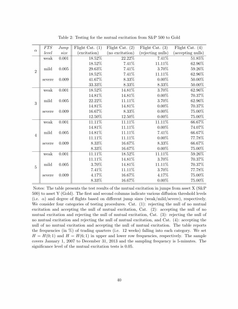
Table 2: Testing for the mutual excitation from S&P 500 to Gold

αFTS Jump Flight Cat. (1) Flight Cat. (2) Flight Cat. (3) Flight Cat. (4)level size (excitation) (no excitation) (rejecting nulls) (accepting nulls)

2

weak 0.001 18.52% 22.22% 7.41% 51.85%18.52% 7.41% 11.11% 62.96%

mild 0.005 29.63% 7.41% 3.70% 59.26%18.52% 7.41% 11.11% 62.96%

severe 0.009 41.67% 8.33% 0.00% 50.00%33.33% 8.33% 8.33% 50.00%

3

weak 0.001 18.52% 14.81% 3.70% 62.96%14.81% 14.81% 0.00% 70.37%

mild 0.005 22.22% 11.11% 3.70% 62.96%14.81% 14.81% 0.00% 70.37%

severe 0.009 16.67% 8.33% 0.00% 75.00%12.50% 12.50% 0.00% 75.00%

4

weak 0.001 11.11% 11.11% 11.11% 66.67%14.81% 11.11% 0.00% 74.07%

mild 0.005 14.81% 11.11% 7.41% 66.67%11.11% 11.11% 0.00% 77.78%

severe 0.009 8.33% 16.67% 8.33% 66.67%8.33% 16.67% 0.00% 75.00%

5

weak 0.001 11.11% 18.52% 11.11% 59.26%11.11% 14.81% 3.70% 70.37%

mild 0.005 3.70% 14.81% 11.11% 70.37%7.41% 11.11% 3.70% 77.78%

severe 0.009 4.17% 16.67% 4.17% 75.00%8.33% 16.67% 0.00% 75.00%

Notes: The table presents the test results of the mutual excitation in jumps from asset X (S&P500) to asset Y (Gold). The first and second columns indicate various diffusion threshold levels(i.e. α) and degree of flights based on different jump sizes (weak/mild/severe), respectively.We consider four categories of testing procedures. Cat. (1): rejecting the null of no mutualexcitation and accepting the null of mutual excitation, Cat. (2): accepting the null of nomutual excitation and rejecting the null of mutual excitation, Cat. (3): rejecting the null ofno mutual excitation and rejecting the null of mutual excitation, and Cat. (4): accepting thenull of no mutual excitation and accepting the null of mutual excitation. The table reportsthe frequencies (in %) of trading quarters (i.e. 12 weeks) falling into each category. We setH = H(0; 1) and H = H(6; 1) in upper and lower row frequencies, respectively. The samplecovers January 1, 2007 to December 31, 2013 and the sampling frequency is 5-minutes. Thesignificance level of the mutual excitation tests is 0.05.

40

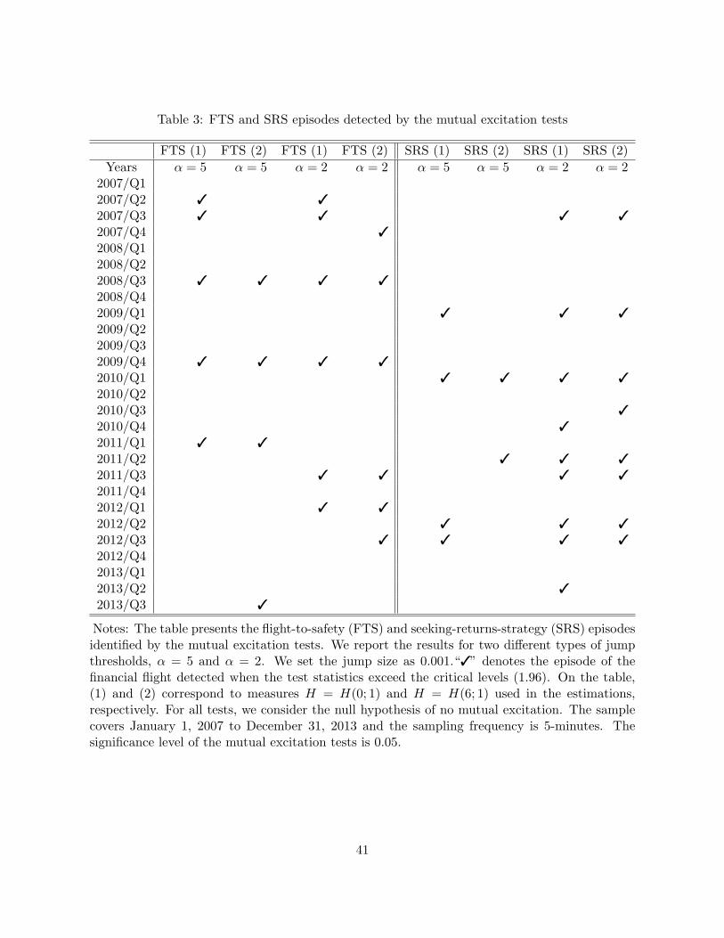
Table 3: FTS and SRS episodes detected by the mutual excitation tests

FTS (1) FTS (2) FTS (1) FTS (2) SRS (1) SRS (2) SRS (1) SRS (2)

Years α = 5 α = 5 α = 2 α = 2 α = 5 α = 5 α = 2 α = 22007/Q12007/Q2

2007/Q3

2007/Q4

2008/Q12008/Q22008/Q3

2008/Q42009/Q1

2009/Q22009/Q32009/Q4

2010/Q1

2010/Q22010/Q3

2010/Q4

2011/Q1

2011/Q2

2011/Q3

2011/Q42012/Q1

2012/Q2

2012/Q3

2012/Q42013/Q12013/Q2

2013/Q3

Notes: The table presents the flight-to-safety (FTS) and seeking-returns-strategy (SRS) episodesidentified by the mutual excitation tests. We report the results for two different types of jumpthresholds, α = 5 and α = 2. We set the jump size as 0.001.“” denotes the episode of thefinancial flight detected when the test statistics exceed the critical levels (1.96). On the table,(1) and (2) correspond to measures H = H(0; 1) and H = H(6; 1) used in the estimations,respectively. For all tests, we consider the null hypothesis of no mutual excitation. The samplecovers January 1, 2007 to December 31, 2013 and the sampling frequency is 5-minutes. Thesignificance level of the mutual excitation tests is 0.05.

41

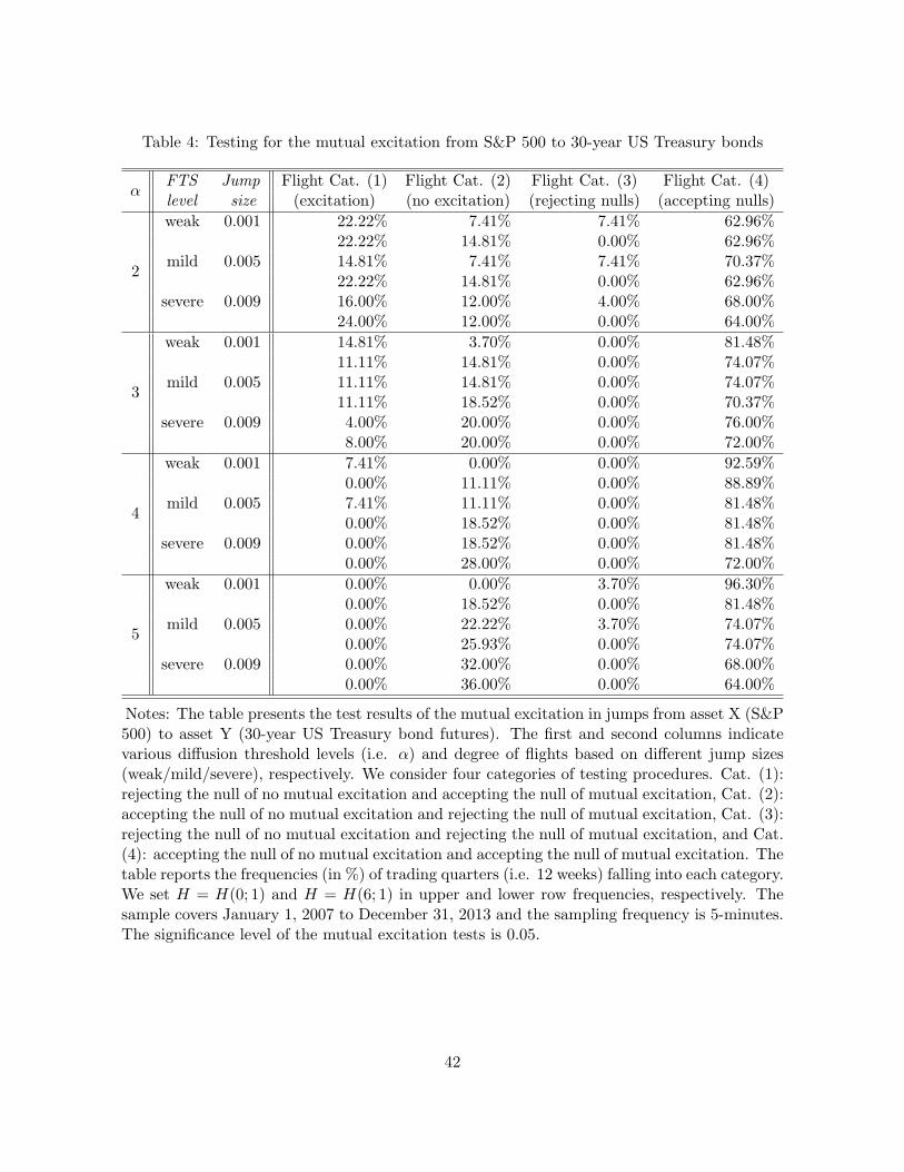
Table 4: Testing for the mutual excitation from S&P 500 to 30-year US Treasury bonds


2

weak 0.001 22.22% 7.41% 7.41% 62.96%22.22% 14.81% 0.00% 62.96%

mild 0.005 14.81% 7.41% 7.41% 70.37%22.22% 14.81% 0.00% 62.96%

severe 0.009 16.00% 12.00% 4.00% 68.00%24.00% 12.00% 0.00% 64.00%

3

weak 0.001 14.81% 3.70% 0.00% 81.48%11.11% 14.81% 0.00% 74.07%

mild 0.005 11.11% 14.81% 0.00% 74.07%11.11% 18.52% 0.00% 70.37%

severe 0.009 4.00% 20.00% 0.00% 76.00%8.00% 20.00% 0.00% 72.00%

4

weak 0.001 7.41% 0.00% 0.00% 92.59%0.00% 11.11% 0.00% 88.89%

mild 0.005 7.41% 11.11% 0.00% 81.48%0.00% 18.52% 0.00% 81.48%

severe 0.009 0.00% 18.52% 0.00% 81.48%0.00% 28.00% 0.00% 72.00%

5

weak 0.001 0.00% 0.00% 3.70% 96.30%0.00% 18.52% 0.00% 81.48%

mild 0.005 0.00% 22.22% 3.70% 74.07%0.00% 25.93% 0.00% 74.07%

severe 0.009 0.00% 32.00% 0.00% 68.00%0.00% 36.00% 0.00% 64.00%

Notes: The table presents the test results of the mutual excitation in jumps from asset X (S&P500) to asset Y (30-year US Treasury bond futures). The first and second columns indicatevarious diffusion threshold levels (i.e. α) and degree of flights based on different jump sizes(weak/mild/severe), respectively. We consider four categories of testing procedures. Cat. (1):rejecting the null of no mutual excitation and accepting the null of mutual excitation, Cat. (2):accepting the null of no mutual excitation and rejecting the null of mutual excitation, Cat. (3):rejecting the null of no mutual excitation and rejecting the null of mutual excitation, and Cat.(4): accepting the null of no mutual excitation and accepting the null of mutual excitation. Thetable reports the frequencies (in %) of trading quarters (i.e. 12 weeks) falling into each category.We set H = H(0; 1) and H = H(6; 1) in upper and lower row frequencies, respectively. Thesample covers January 1, 2007 to December 31, 2013 and the sampling frequency is 5-minutes.The significance level of the mutual excitation tests is 0.05.

42

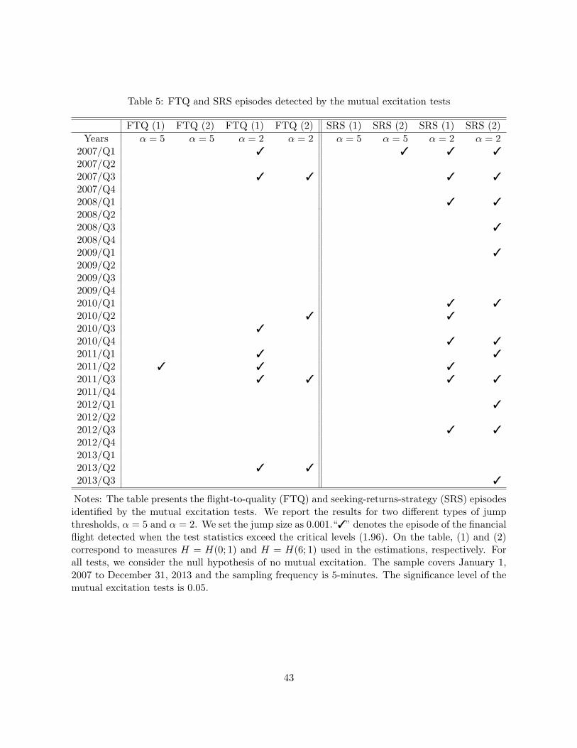
Table 5: FTQ and SRS episodes detected by the mutual excitation tests

FTQ (1) FTQ (2) FTQ (1) FTQ (2) SRS (1) SRS (2) SRS (1) SRS (2)

Years α = 5 α = 5 α = 2 α = 2 α = 5 α = 5 α = 2 α = 22007/Q1

2007/Q22007/Q3

2007/Q42008/Q1

2008/Q22008/Q3

2008/Q42009/Q1

2009/Q22009/Q32009/Q42010/Q1

2010/Q2

2010/Q3

2010/Q4

2011/Q1

2011/Q2

2011/Q3

2011/Q42012/Q1

2012/Q22012/Q3

2012/Q42013/Q12013/Q2

2013/Q3

Notes: The table presents the flight-to-quality (FTQ) and seeking-returns-strategy (SRS) episodesidentified by the mutual excitation tests. We report the results for two different types of jumpthresholds, α = 5 and α = 2. We set the jump size as 0.001.“” denotes the episode of the financialflight detected when the test statistics exceed the critical levels (1.96). On the table, (1) and (2)correspond to measures H = H(0; 1) and H = H(6; 1) used in the estimations, respectively. Forall tests, we consider the null hypothesis of no mutual excitation. The sample covers January 1,2007 to December 31, 2013 and the sampling frequency is 5-minutes. The significance level of themutual excitation tests is 0.05.

43

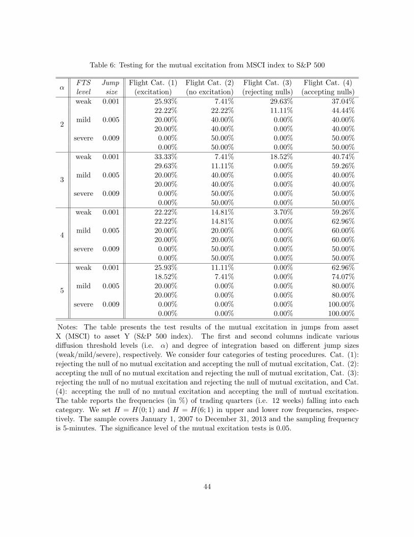
Table 6: Testing for the mutual excitation from MSCI index to S&P 500


2

weak 0.001 25.93% 7.41% 29.63% 37.04%22.22% 22.22% 11.11% 44.44%

mild 0.005 20.00% 40.00% 0.00% 40.00%20.00% 40.00% 0.00% 40.00%

severe 0.009 0.00% 50.00% 0.00% 50.00%0.00% 50.00% 0.00% 50.00%

3

weak 0.001 33.33% 7.41% 18.52% 40.74%29.63% 11.11% 0.00% 59.26%

mild 0.005 20.00% 40.00% 0.00% 40.00%20.00% 40.00% 0.00% 40.00%

severe 0.009 0.00% 50.00% 0.00% 50.00%0.00% 50.00% 0.00% 50.00%

4

weak 0.001 22.22% 14.81% 3.70% 59.26%22.22% 14.81% 0.00% 62.96%

mild 0.005 20.00% 20.00% 0.00% 60.00%20.00% 20.00% 0.00% 60.00%

severe 0.009 0.00% 50.00% 0.00% 50.00%0.00% 50.00% 0.00% 50.00%

5

weak 0.001 25.93% 11.11% 0.00% 62.96%18.52% 7.41% 0.00% 74.07%

mild 0.005 20.00% 0.00% 0.00% 80.00%20.00% 0.00% 0.00% 80.00%

severe 0.009 0.00% 0.00% 0.00% 100.00%0.00% 0.00% 0.00% 100.00%

Notes: The table presents the test results of the mutual excitation in jumps from assetX (MSCI) to asset Y (S&P 500 index). The first and second columns indicate variousdiffusion threshold levels (i.e. α) and degree of integration based on different jump sizes(weak/mild/severe), respectively. We consider four categories of testing procedures. Cat. (1):rejecting the null of no mutual excitation and accepting the null of mutual excitation, Cat. (2):accepting the null of no mutual excitation and rejecting the null of mutual excitation, Cat. (3):rejecting the null of no mutual excitation and rejecting the null of mutual excitation, and Cat.(4): accepting the null of no mutual excitation and accepting the null of mutual excitation.The table reports the frequencies (in %) of trading quarters (i.e. 12 weeks) falling into eachcategory. We set H = H(0; 1) and H = H(6; 1) in upper and lower row frequencies, respec-tively. The sample covers January 1, 2007 to December 31, 2013 and the sampling frequencyis 5-minutes. The significance level of the mutual excitation tests is 0.05.

44

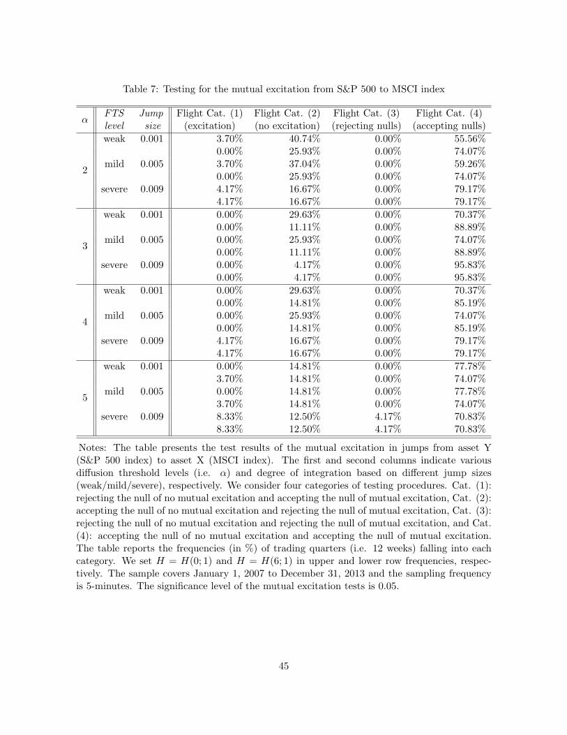
Table 7: Testing for the mutual excitation from S&P 500 to MSCI index


2

weak 0.001 3.70% 40.74% 0.00% 55.56%0.00% 25.93% 0.00% 74.07%

mild 0.005 3.70% 37.04% 0.00% 59.26%0.00% 25.93% 0.00% 74.07%

severe 0.009 4.17% 16.67% 0.00% 79.17%4.17% 16.67% 0.00% 79.17%

3

weak 0.001 0.00% 29.63% 0.00% 70.37%0.00% 11.11% 0.00% 88.89%

mild 0.005 0.00% 25.93% 0.00% 74.07%0.00% 11.11% 0.00% 88.89%

severe 0.009 0.00% 4.17% 0.00% 95.83%0.00% 4.17% 0.00% 95.83%

4

weak 0.001 0.00% 29.63% 0.00% 70.37%0.00% 14.81% 0.00% 85.19%

mild 0.005 0.00% 25.93% 0.00% 74.07%0.00% 14.81% 0.00% 85.19%

severe 0.009 4.17% 16.67% 0.00% 79.17%4.17% 16.67% 0.00% 79.17%

5

weak 0.001 0.00% 14.81% 0.00% 77.78%3.70% 14.81% 0.00% 74.07%

mild 0.005 0.00% 14.81% 0.00% 77.78%3.70% 14.81% 0.00% 74.07%

severe 0.009 8.33% 12.50% 4.17% 70.83%8.33% 12.50% 4.17% 70.83%

Notes: The table presents the test results of the mutual excitation in jumps from asset Y(S&P 500 index) to asset X (MSCI index). The first and second columns indicate variousdiffusion threshold levels (i.e. α) and degree of integration based on different jump sizes(weak/mild/severe), respectively. We consider four categories of testing procedures. Cat. (1):rejecting the null of no mutual excitation and accepting the null of mutual excitation, Cat. (2):accepting the null of no mutual excitation and rejecting the null of mutual excitation, Cat. (3):rejecting the null of no mutual excitation and rejecting the null of mutual excitation, and Cat.(4): accepting the null of no mutual excitation and accepting the null of mutual excitation.The table reports the frequencies (in %) of trading quarters (i.e. 12 weeks) falling into eachcategory. We set H = H(0; 1) and H = H(6; 1) in upper and lower row frequencies, respec-tively. The sample covers January 1, 2007 to December 31, 2013 and the sampling frequencyis 5-minutes. The significance level of the mutual excitation tests is 0.05.

45

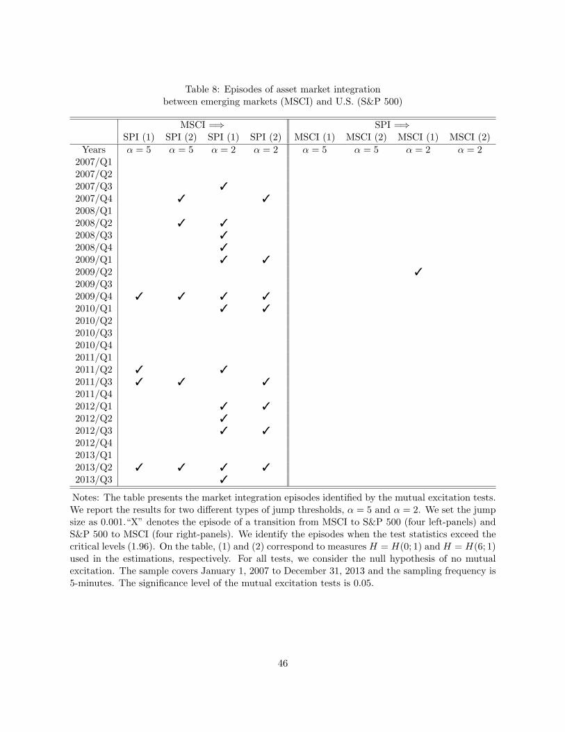
Table 8: Episodes of asset market integrationbetween emerging markets (MSCI) and U.S. (S&P 500)

MSCI =⇒ SPI =⇒SPI (1) SPI (2) SPI (1) SPI (2) MSCI (1) MSCI (2) MSCI (1) MSCI (2)

Years α = 5 α = 5 α = 2 α = 2 α = 5 α = 5 α = 2 α = 22007/Q12007/Q22007/Q3

2007/Q4

2008/Q12008/Q2

2008/Q3

2008/Q4

2009/Q1

2009/Q2

2009/Q32009/Q4

2010/Q1

2010/Q22010/Q32010/Q42011/Q12011/Q2

2011/Q3

2011/Q42012/Q1

2012/Q2

2012/Q3

2012/Q42013/Q12013/Q2

2013/Q3

Notes: The table presents the market integration episodes identified by the mutual excitation tests.We report the results for two different types of jump thresholds, α = 5 and α = 2. We set the jumpsize as 0.001.“X” denotes the episode of a transition from MSCI to S&P 500 (four left-panels) andS&P 500 to MSCI (four right-panels). We identify the episodes when the test statistics exceed thecritical levels (1.96). On the table, (1) and (2) correspond to measures H = H(0; 1) and H = H(6; 1)used in the estimations, respectively. For all tests, we consider the null hypothesis of no mutualexcitation. The sample covers January 1, 2007 to December 31, 2013 and the sampling frequency is5-minutes. The significance level of the mutual excitation tests is 0.05.

46

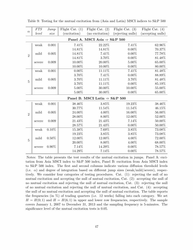
Table 9: Testing for the mutual excitation from (Asia and Latin) MSCI indices to S&P 500


Panel A. MSCI Asia ⇒ S&P 500

2

weak 0.001 7.41% 22.22% 7.41% 62.96%14.81% 14.81% 0.00% 70.37%

mild 0.005 14.81% 7.41% 0.00% 77.78%14.81% 3.70% 0.00% 81.48%

severe 0.009 10.00% 20.00% 5.00% 65.00%10.00% 10.00% 0.00% 80.00%

5

weak 0.001 0.00% 11.11% 7.41% 81.48%3.70% 7.41% 0.00% 88.89%

mild 0.005 3.70% 11.11% 3.70% 81.48%3.70% 11.11% 0.00% 85.19%

severe 0.009 5.00% 30.00% 10.00% 55.00%5.00% 30.00% 0.00% 65.00%

Panel B. MSCI Latin ⇒ S&P 500

2

weak 0.001 38.46% 3.85% 19.23% 38.46%30.77% 11.54% 11.54% 46.15%

mild 0.005 24.00% 4.00% 16.00% 56.00%28.00% 8.00% 12.00% 52.00%

severe 0.009 21.43% 21.43% 7.14% 50.00%28.57% 21.43% 0.00% 50.00%

5

weak 0.10% 15.38% 7.69% 3.85% 73.08%19.23% 3.85% 3.85% 73.08%

mild 0.50% 12.00% 12.00% 4.00% 72.00%20.00% 8.00% 4.00% 68.00%

severe 0.90% 7.14% 14.29% 0.00% 78.57%14.29% 7.14% 0.00% 78.57%

Notes: The table presents the test results of the mutual excitation in jumps. Panel A: exci-tation from Asia MSCI index to S&P 500 index, Panel B: excitation from Asia MSCI indexto S&P 500 index. The first and second columns indicate various diffusion threshold levels(i.e. α) and degree of integration based on different jump sizes (weak/mild/severe), respec-tively. We consider four categories of testing procedures. Cat. (1): rejecting the null of nomutual excitation and accepting the null of mutual excitation, Cat. (2): accepting the null ofno mutual excitation and rejecting the null of mutual excitation, Cat. (3): rejecting the nullof no mutual excitation and rejecting the null of mutual excitation, and Cat. (4): acceptingthe null of no mutual excitation and accepting the null of mutual excitation. The table reportsthe frequencies (in %) of trading quarters (i.e. 12 weeks) falling into each category. We setH = H(0; 1) and H = H(6; 1) in upper and lower row frequencies, respectively. The samplecovers January 1, 2007 to December 31, 2013 and the sampling frequency is 5-minutes. Thesignificance level of the mutual excitation tests is 0.05.

47

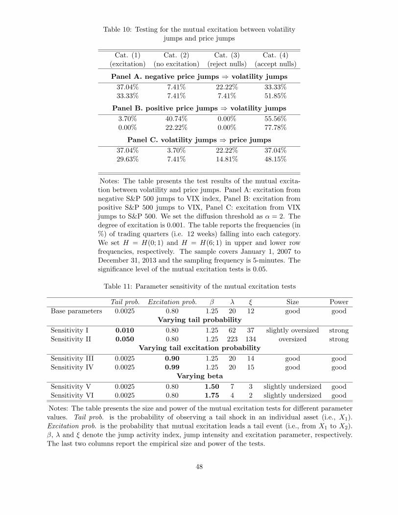
Table 10: Testing for the mutual excitation between volatilityjumps and price jumps

Cat. (1) Cat. (2) Cat. (3) Cat. (4)(excitation) (no excitation) (reject nulls) (accept nulls)

Panel A. negative price jumps ⇒ volatility jumps

37.04% 7.41% 22.22% 33.33%33.33% 7.41% 7.41% 51.85%

Panel B. positive price jumps ⇒ volatility jumps

3.70% 40.74% 0.00% 55.56%0.00% 22.22% 0.00% 77.78%

Panel C. volatility jumps ⇒ price jumps

37.04% 3.70% 22.22% 37.04%29.63% 7.41% 14.81% 48.15%

Notes: The table presents the test results of the mutual excita-tion between volatility and price jumps. Panel A: excitation fromnegative S&P 500 jumps to VIX index, Panel B: excitation frompositive S&P 500 jumps to VIX, Panel C: excitation from VIXjumps to S&P 500. We set the diffusion threshold as α = 2. Thedegree of excitation is 0.001. The table reports the frequencies (in%) of trading quarters (i.e. 12 weeks) falling into each category.We set H = H(0; 1) and H = H(6; 1) in upper and lower rowfrequencies, respectively. The sample covers January 1, 2007 toDecember 31, 2013 and the sampling frequency is 5-minutes. Thesignificance level of the mutual excitation tests is 0.05.

Table 11: Parameter sensitivity of the mutual excitation tests

Tail prob. Excitation prob. β λ ξ Size Power

Base parameters 0.0025 0.80 1.25 20 12 good goodVarying tail probability

Sensitivity I 0.010 0.80 1.25 62 37 slightly oversized strongSensitivity II 0.050 0.80 1.25 223 134 oversized strong

Varying tail excitation probability

Sensitivity III 0.0025 0.90 1.25 20 14 good goodSensitivity IV 0.0025 0.99 1.25 20 15 good good

Varying beta

Sensitivity V 0.0025 0.80 1.50 7 3 slightly undersized goodSensitivity VI 0.0025 0.80 1.75 4 2 slightly undersized good

Notes: The table presents the size and power of the mutual excitation tests for different parametervalues. Tail prob. is the probability of observing a tail shock in an individual asset (i.e., X1).Excitation prob. is the probability that mutual excitation leads a tail event (i.e., from X1 to X2).β, λ and ξ denote the jump activity index, jump intensity and excitation parameter, respectively.The last two columns report the empirical size and power of the tests.

48

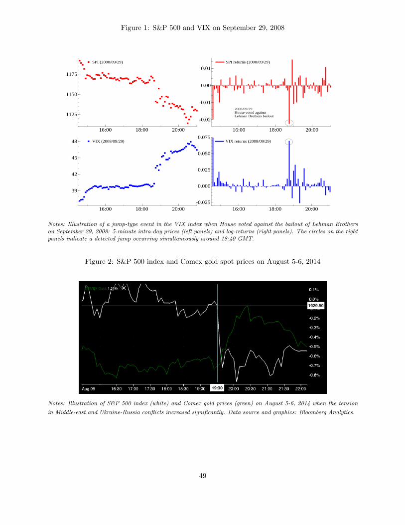
Figure 1: S&P 500 and VIX on September 29, 2008

SPI (2008/09/29)

16:00 18:00 20:00

1125

1150

1175

SPI (2008/09/29) SPI returns (2008/09/29)

16:00 18:00 20:00

-0.02

-0.01

0.00

0.01

2008/09/29House voted against Lehman Brothers bailout

SPI returns (2008/09/29)

VIX (2008/09/29)

16:00 18:00 20:00

39

42

45

48 VIX (2008/09/29) VIX returns (2008/09/29)

16:00 18:00 20:00-0.025

0.000

0.025

0.050

0.075VIX returns (2008/09/29)

Notes: Illustration of a jump-type event in the VIX index when House voted against the bailout of Lehman Brotherson September 29, 2008: 5-minute intra-day prices (left panels) and log-returns (right panels). The circles on the rightpanels indicate a detected jump occurring simultaneously around 18:40 GMT.

Figure 2: S&P 500 index and Comex gold spot prices on August 5-6, 2014

Notes: Illustration of S&P 500 index (white) and Comex gold prices (green) on August 5-6, 2014 when the tension

in Middle-east and Ukraine-Russia conflicts increased significantly. Data source and graphics: Bloomberg Analytics.

49

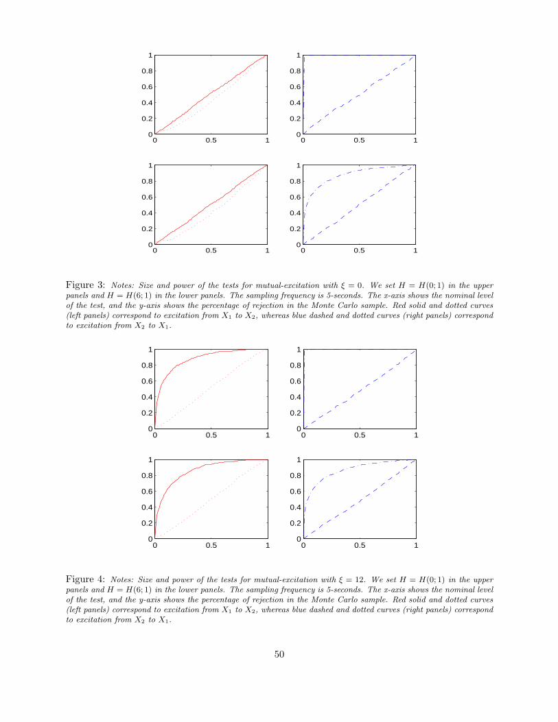
0 0.5 10

0.2

0.4

0.6

0.8

1

0 0.5 10

0.2

0.4

0.6

0.8

1

0 0.5 10

0.2

0.4

0.6

0.8

1

0 0.5 10

0.2

0.4

0.6

0.8

1

Figure 3: Notes: Size and power of the tests for mutual-excitation with ξ = 0. We set H = H(0; 1) in the upperpanels and H = H(6; 1) in the lower panels. The sampling frequency is 5-seconds. The x-axis shows the nominal levelof the test, and the y-axis shows the percentage of rejection in the Monte Carlo sample. Red solid and dotted curves(left panels) correspond to excitation from X1 to X2, whereas blue dashed and dotted curves (right panels) correspondto excitation from X2 to X1.

0 0.5 10

0.2

0.4

0.6

0.8

1

0 0.5 10

0.2

0.4

0.6

0.8

1

0 0.5 10

0.2

0.4

0.6

0.8

1

0 0.5 10

0.2

0.4

0.6

0.8

1

Figure 4: Notes: Size and power of the tests for mutual-excitation with ξ = 12. We set H = H(0; 1) in the upperpanels and H = H(6; 1) in the lower panels. The sampling frequency is 5-seconds. The x-axis shows the nominal levelof the test, and the y-axis shows the percentage of rejection in the Monte Carlo sample. Red solid and dotted curves(left panels) correspond to excitation from X1 to X2, whereas blue dashed and dotted curves (right panels) correspondto excitation from X2 to X1.

50

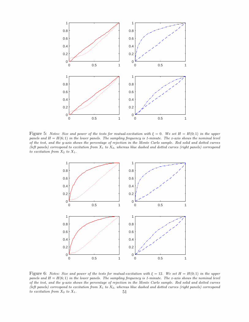
0 0.5 10

0.2

0.4

0.6

0.8

1

0 0.5 10

0.2

0.4

0.6

0.8

1

0 0.5 10

0.2

0.4

0.6

0.8

1

0 0.5 10

0.2

0.4

0.6

0.8

1

Figure 5: Notes: Size and power of the tests for mutual-excitation with ξ = 0. We set H = H(0; 1) in the upperpanels and H = H(6; 1) in the lower panels. The sampling frequency is 1-minute. The x-axis shows the nominal levelof the test, and the y-axis shows the percentage of rejection in the Monte Carlo sample. Red solid and dotted curves(left panels) correspond to excitation from X1 to X2, whereas blue dashed and dotted curves (right panels) correspondto excitation from X2 to X1.

0 0.5 10

0.2

0.4

0.6

0.8

1

0 0.5 10

0.2

0.4

0.6

0.8

1

0 0.5 10

0.2

0.4

0.6

0.8

1

0 0.5 10

0.2

0.4

0.6

0.8

1

Figure 6: Notes: Size and power of the tests for mutual-excitation with ξ = 12. We set H = H(0; 1) in the upperpanels and H = H(6; 1) in the lower panels. The sampling frequency is 1-minute. The x-axis shows the nominal levelof the test, and the y-axis shows the percentage of rejection in the Monte Carlo sample. Red solid and dotted curves(left panels) correspond to excitation from X1 to X2, whereas blue dashed and dotted curves (right panels) correspondto excitation from X2 to X1. 51

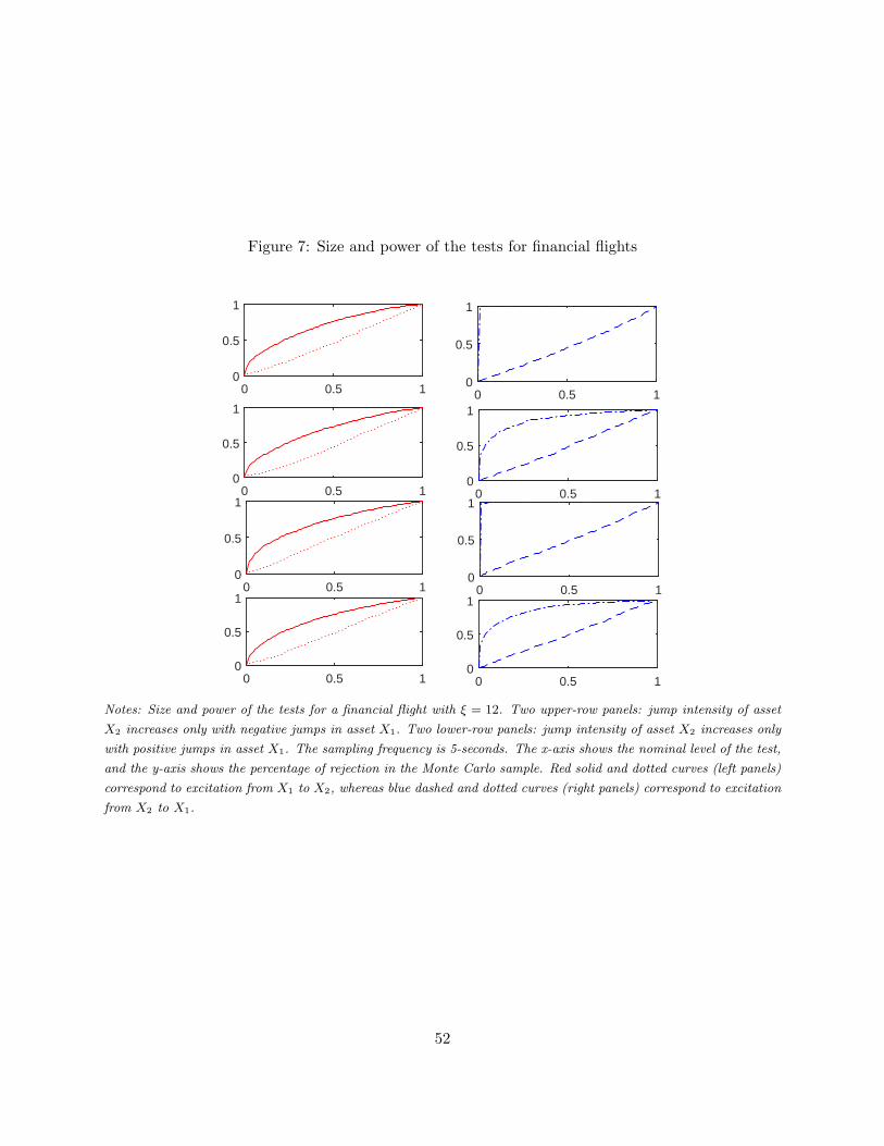
Figure 7: Size and power of the tests for financial flights

0 0.5 10

0.5

1

0 0.5 10

0.5

1

0 0.5 10

0.5

1

0 0.5 10

0.5

1

0 0.5 10

0.5

1

0 0.5 10

0.5

10 0.5 1

0

0.5

1

0 0.5 10

0.5

1

Notes: Size and power of the tests for a financial flight with ξ = 12. Two upper-row panels: jump intensity of asset

X2 increases only with negative jumps in asset X1. Two lower-row panels: jump intensity of asset X2 increases only

with positive jumps in asset X1. The sampling frequency is 5-seconds. The x-axis shows the nominal level of the test,

and the y-axis shows the percentage of rejection in the Monte Carlo sample. Red solid and dotted curves (left panels)

correspond to excitation from X1 to X2, whereas blue dashed and dotted curves (right panels) correspond to excitation

from X2 to X1.

52

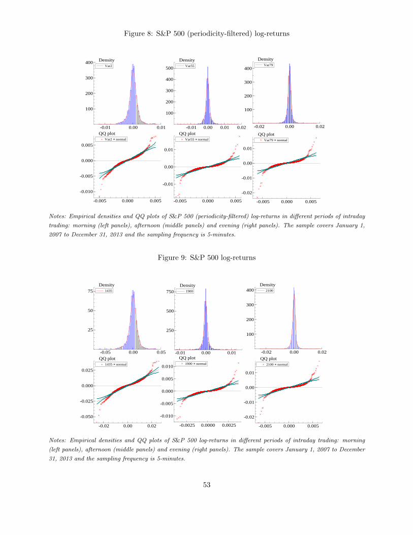
Figure 8: S&P 500 (periodicity-filtered) log-returns

Var2

-0.01 0.00 0.01

100

200

300

400 DensityVar2

Var2 × normal

-0.005 0.000 0.005

-0.010

-0.005

0.000

0.005

QQ plotVar2 × normal

Var55

-0.01 0.00 0.01 0.02

100

200

300

400

500

DensityVar55

Var55 × normal

-0.005 0.000 0.005

-0.01

0.00

0.01


Var79

-0.02 0.00 0.02

100

200

300

400

DensityVar79

Var79 × normal

-0.005 0.000 0.005

-0.02

-0.01

0.00

0.01


Notes: Empirical densities and QQ plots of S&P 500 (periodicity-filtered) log-returns in different periods of intraday

trading: morning (left panels), afternoon (middle panels) and evening (right panels). The sample covers January 1,

2007 to December 31, 2013 and the sampling frequency is 5-minutes.

Figure 9: S&P 500 log-returns

1435

-0.05 0.00 0.05

25

50

75Density

1435

1435 × normal

-0.02 0.00 0.02

-0.050

-0.025

0.000

0.025

QQ plot1435 × normal

1900

-0.01 0.00 0.01

250

500

750Density

1900

1900 × normal

-0.0025 0.0000 0.0025

-0.010

-0.005

0.000

0.005

0.010


2100

-0.02 0.00 0.02

100

200

300

400Density

2100

2100 × normal

-0.005 0.000 0.005

-0.02

-0.01

0.00

0.01


Notes: Empirical densities and QQ plots of S&P 500 log-returns in different periods of intraday trading: morning

(left panels), afternoon (middle panels) and evening (right panels). The sample covers January 1, 2007 to December

31, 2013 and the sampling frequency is 5-minutes.

53

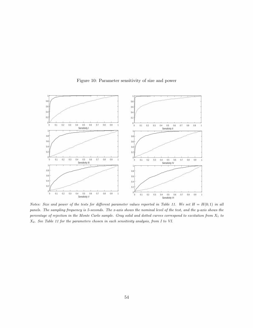
Figure 10: Parameter sensitivity of size and power

Sensitivity I0 0.1 0.2 0.3 0.4 0.5 0.6 0.7 0.8 0.9 1

0

0.2

0.4

0.6

0.8

1

Sensitivity II0 0.1 0.2 0.3 0.4 0.5 0.6 0.7 0.8 0.9 1

0

0.2

0.4

0.6

0.8

1

Sensitivity III0 0.1 0.2 0.3 0.4 0.5 0.6 0.7 0.8 0.9 1

0

0.2

0.4

0.6

0.8

1

Sensitivity IV0 0.1 0.2 0.3 0.4 0.5 0.6 0.7 0.8 0.9 1

0

0.2

0.4

0.6

0.8

1

Sensitivity V0 0.1 0.2 0.3 0.4 0.5 0.6 0.7 0.8 0.9 1

0

0.2

0.4

0.6

0.8

1

Sensitivity VI0 0.1 0.2 0.3 0.4 0.5 0.6 0.7 0.8 0.9 1

0

0.2

0.4

0.6

0.8

1

Notes: Size and power of the tests for different parameter values reported in Table 11. We set H = H(0; 1) in all

panels. The sampling frequency is 5-seconds. The x-axis shows the nominal level of the test, and the y-axis shows the

percentage of rejection in the Monte Carlo sample. Gray solid and dotted curves correspond to excitation from X1 to

X2. See Table 11 for the parameters chosen in each sensitivity analysis, from I to VI.

54

financial flights, stock market linkages and jump excitation

Documents