The Firm and the Market

MICROECONOMICS

Principles and Analysis

Frank Cowell

Almost essential

Firm: Demand and Supply

PrerequisitesPrerequisites

October 2005

Introduction

� In previous presentations we’ve seen how an optimising agent reacts to the market.

� Use the comparative statics method

� We could now extend this to other similar problems.

� But first a useful exercise in microeconomics:

� Relax the special assumptions

� We will do this in two stages:

� Move from one price-taking firm to many

� Drop the assumption of price-taking behaviour.

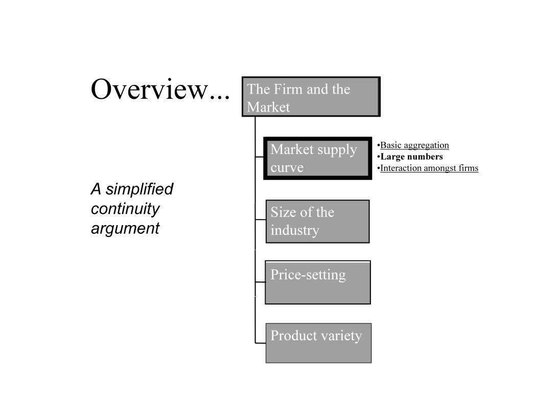
Overview...

Market supply

curve

Size of the

industry

Price-setting

Product variety

The Firm and the

Market

Issues in

aggregating

supply curves of

price-taking firms

•Basic aggregation

•Large numbers

•Interaction amongst firms

Aggregation over firms

� We begin with a very simple model.

� Two firms with similar cost structures.

� But using a very special assumption.

� First we look at the method of getting the

market supply curve.

� Then note the shortcomings of our

particular example.

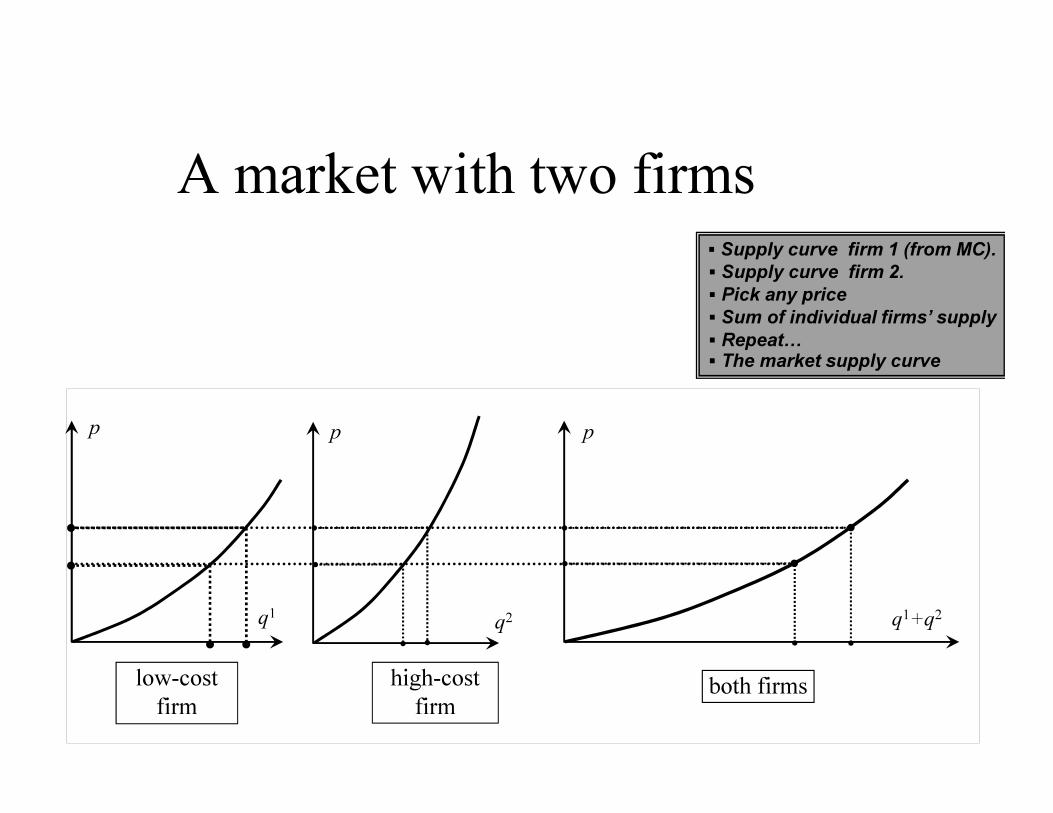
A market with two firms

q1

p

low-cost

firm

q2

p

high-cost

firm

p

q1+q2

both firms

� Supply curve firm 1 (from MC).

� Supply curve firm 2.

� Pick any price

� Sum of individual firms’ supply

� Repeat�� The market supply curve

•

•

Simple aggregation

� Individual firm supply curves derived from MC curves

� “Horizontal summation” of supply curves

� Market supply curve is flatter than supply curve for

each firm

� But the story is a little strange:

1. Each firm act as a price taker even though there is

just one other firm in the market.

2. Number of firms is fixed (in this case at 2).

3. Firms' supply curve is different from that in

previous presentationsTry another

example

See presentation

on duopoly

Later in this

presentation

Another simple case

� Two price-taking firms.

� Similar “piecewise linear” MC curves:

� Each firm has a fixed cost.

� Marginal cost rises at the same constant rate.

� Firm 1 is the low-cost firm.

� Analyse the supply of these firms over three

price ranges.

Follow the

procedure again

Market supply curve (2)

low-cost

firm

p'

high-cost

firm

p"

p'

both firms

p"

Now for a

problem

q1 q2 q1+q2

� Below p' neither firm is in the

market

� Between p' and p'' only firm 1

is in the market

� Above p'' both firms are in the

market

•

• •

•

•

pp p

Where is the market equilibrium?

� Try p′ (demand exceeds

supply )

supply

demandp

q

p"

p′

p′″

� Try p″′ (supply exceeds

demand)

� There is no

equilibrium at p"

Lesson 1

� Nonconcave production function can lead to

discontinuity in supply function.

� Discontinuity in supply functions may mean

that there is no equilibrium.

Overview...

Market supply

curve

Size of the

industry

Price-setting

Product variety

The Firm and the

Market

A simplified

continuity

argument

•Basic aggregation

•Large numbers

•Interaction amongst firms

A further experiment

� The problem of nonexistent equilibrium

arose from discontinuity in supply.

� But is discontinuity likely to be a serious

problem?

� Let’s go through another example.� Similar cost function to previous case

� This time − identical firms

� (Not essential – but it’s easier to follow)

Take two identical firms...

p'

p

4 8 12 16

q1

p'

p

4 8 12 16

q2

Sum to get aggregate supply

24 328 16

p'

p

q1 +q2

•

•• • • •• •••

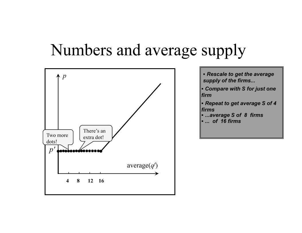
Numbers and average supply

p

4 8 12 16

average(qf)

p'

� Rescale to get the average

supply of the firms...

� Compare with S for just one

firm

� Repeat to get average S of 4

firms� ...average S of 8 firms� ... of 16 firms

••• •• •

There’s an

extra dot!Two more

dots!

The limiting case

p

4 8 12 16

average(qf)

p'

� In the limit draw a continuous

“averaged” supply curve

� A solution to the non-

existence problem?

� A well-defined equilibrium

(3/16)N of the firms at q=0

(13/16)N of the firms at q=16.

average

supply

average

demand

� Firms’ outputs in equilibrium

Lesson 2

� A further insight into nonconcavity of production function (nonconvexity of production possibilities).

� Yes, nonconvexities can lead to problems:

� Discontinuity of response function.

� Nonexistence of equilibrium.

� But if there are large numbers of firms then then we may have a solution.

� The average behaviour may appear to be conventional.

Overview...

Market supply

curve

Size of the

industry

Price-setting

Product variety

The Firm and the

Market

Introducing

“externalities”

•Basic aggregation

•Large numbers

•Interaction amongst firms

Interaction amongst firms

� Consider two main types of interaction

� Negative externalities� Pollution

� Congestion

� …

� Positive externalities � Training

� Networking

� Infrastructure

� Other interactions?� For example, effects of one firm on input prices of other firms

� Normal multimarket equilibrium

� Not relevant here

Industry supply: negative

externality

S

S2 (q1=1)

S2 (q1=5)

S1 (q2=1)

S1 (q2=5)

MC1+MC2

q2

firm 2 alone

p

MC1+MC2

both firms

q1+ q2

p

q1

firm 1 alone

p

� Each firm’s S-curve (MC)

shifted by the other’s output

� The result of simple ΣMC at

each output level

� Industry supply allowing for

interaction.

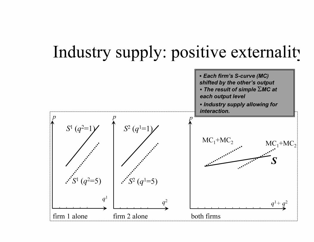
Industry supply: positive externality

S

S2 (q1=1)

S2 (q1=5)

S1 (q2=1)

S1 (q2=5)

MC1+MC2

q2

firm 2 alone

p

MC1+MC2

both firms

q1+ q2

p

q1

firm 1 alone

p

� Each firm’s S-curve (MC)

shifted by the other’s output

� The result of simple ΣMC at

each output level

� Industry supply allowing for

interaction.

Positive externality: extreme case

S

MC1+MC2

MC1+MC2

both firms

q1+ q2

p

Externality and supply: summary

� Externalities affect properties of response function.

� Negative externality:� Supply less responsive than the “sum-of-the-

MC” rule indicates.

� Positive externality:� Supply more responsive than the “sum-of-the-

MC” rule indicates.

� Could have forward-falling supply curve.

Overview...

Market supply

curve

Size of the

industry

Price-setting

Product variety

The Firm and the

Market

Determining the

equilibrium

number of firms

The issue

� Previous argument has taken given number of firms.

� This is unsatisfactory:� How is the number to be fixed?

� Should be determined within the model

� …by economic behaviour of firms

� …by conditions in the market.

� Look at the “entry mechanism.”� Base this on previous model

� Must be consistent with equilibrium behaviour

� So, begin with equilibrium conditions for a single firm…

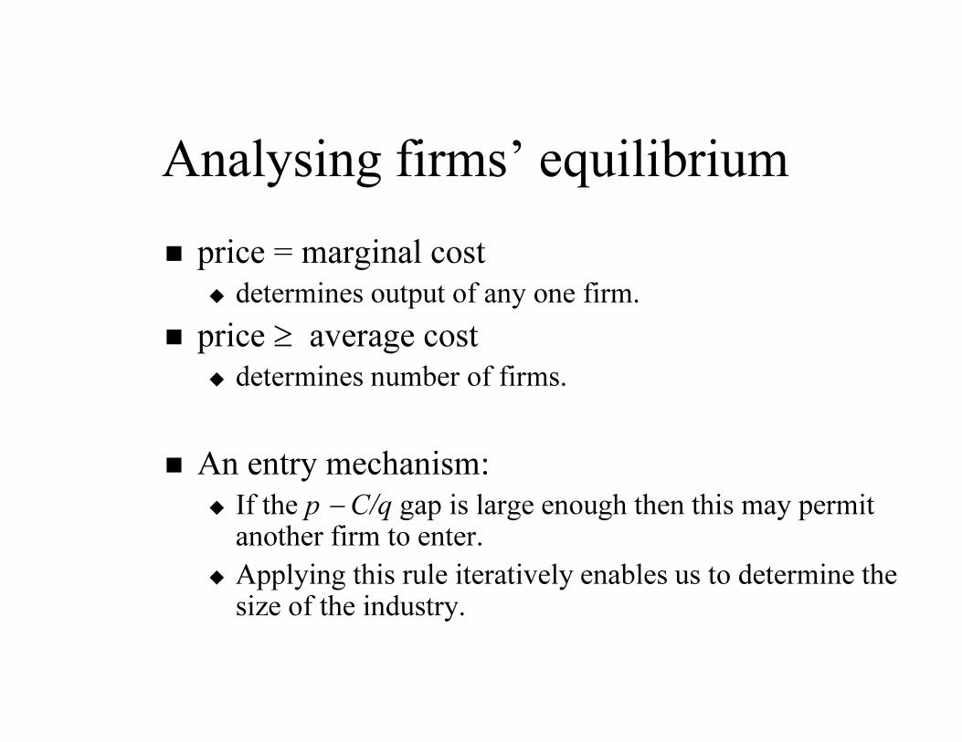
Analysing firms’ equilibrium

� price = marginal cost

� determines output of any one firm.

� price ≥ average cost

� determines number of firms.

� An entry mechanism:

� If the p − C/q gap is large enough then this may permit another firm to enter.

� Applying this rule iteratively enables us to determine the size of the industry.

Outline of the process

� (0) Assume that firm 1 makes a positive profit

� (1) Is pq – C ≤ set-up costs of a new firm?� ...if YES then stop. We’ve got the eqm # of firms

� ...otherwise continue:

� (2) Number of firms goes up by 1

� (3) Industry output goes up

� (4) Price falls (D-curve) and individual firms

adjust output (individual firm’s S-curve)

� (5) Back to step 1

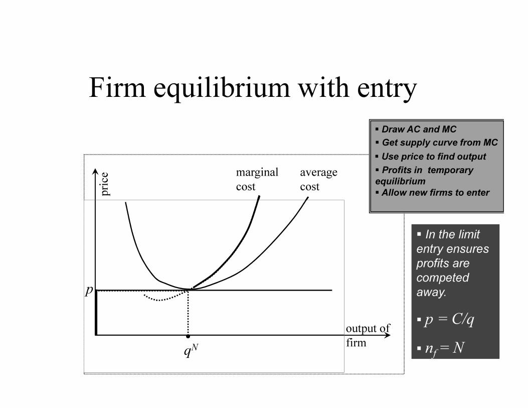
Firm equilibrium with entry

marginal

cost

average

cost

output of

firm

p

q1

Π1

price

� Draw AC and MC

� Get supply curve from MC

� Use price to find output

� Profits in temporary

equilibrium

� Price-taking

temporary

equilibrium

� nf = 1

� Allow new firms to enter

p

q2

2

p

q3

34

p

q4

p

qN

� In the limit

entry ensures

profits are

competed

away.

� p = C/q

� nf = N

Overview...

Market supply

curve

Size of the

industry

Price-setting

Product variety

The Firm and the

Market

The economic

analysis of

monopoly

The issues

� We've taken for granted a firm's environment.

� What basis for the given price assumption?

� What if we relax it for a single firm?

� Get the classic model of monopoly:

� An elementary story of market power

� A bit strange − what ensures there is only one firm?

� The basis for many other models of the firm.

A simple price-setting firm

� Compare with the price-taking firm.

� Output price is no longer exogenous.

� We assume a determinate demand curve.

� No other firm’s actions are relevant.

� Profit maximisation is still the objective.

Monopoly – model structure

� We are given the inverse demand function:� p = p(q)

� Gives the price that rules if the monopolist delivers q to the market.

� For obvious reasons, consider it as the average revenue curve (AR).

� Total revenue is: � p(q)q.

� Differentiate to get monopolist’s marginal revenue (MR):� p(q)+pq(q)q

� pq(•) means dp(•)/dq

� Clearly, if pq(q) is negative (demand curve is downward

sloping), then MR < AR.

Average and marginal revenue

q

p

p(q)

AR

p(q)q

�AR curve is just the

market demand curve...

�Total revenue: area in the

rectangle underneath

�Differentiate total revenue

to get marginal revenue

MR

dp(q)qdq

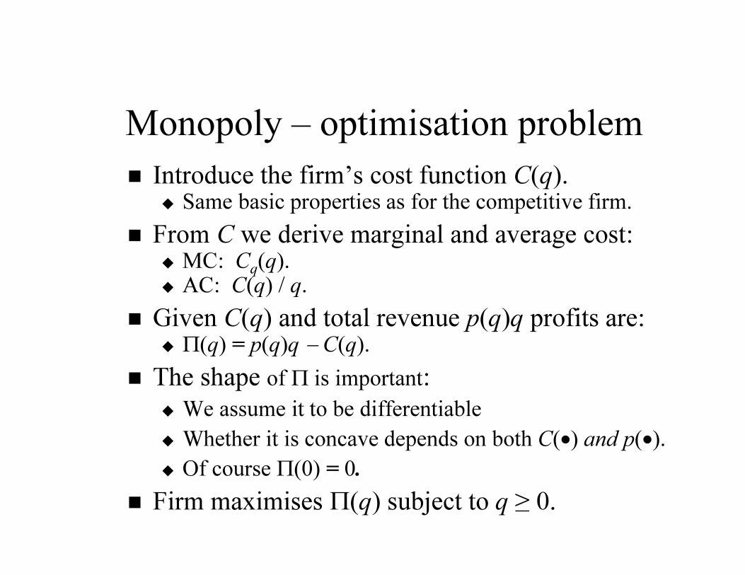
Monopoly – optimisation problem

� Introduce the firm’s cost function C(q).� Same basic properties as for the competitive firm.

� From C we derive marginal and average cost:� MC: Cq(q).� AC: C(q) / q.

� Given C(q) and total revenue p(q)q profits are: � Π(q) = p(q)q − C(q).

� The shape of Π is important:

� We assume it to be differentiable

� Whether it is concave depends on both C(•) and p(•).

� Of course Π(0) = 0.

� Firm maximises Π(q) subject to q ≥ 0.

Monopoly – solving the problem� Problem is “max Π(q) s.t. q ≥ 0,” where:

� Π(q) = p(q)q − C(q).

� First- and second-order conditions for interior maximum:� Πq (q) = 0.

� Πqq (q) < 0.

� Evaluating the FOC:� p(q) + pq(q)q − Cq(q) = 0.

� Rearrange this: � p(q) + pq(q)q = Cq(q)

� “Marginal Revenue = Marginal Cost”

� This condition gives the solution.� From above get optimal output q* .

� Put q* in p(•) to get monopolist’s price:

� p* = p(q* ).

� Check this diagrammatically…

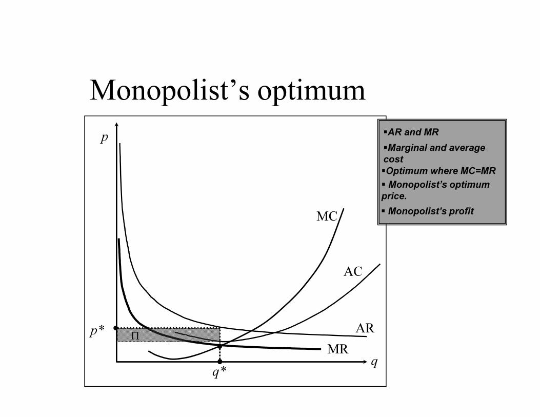
Monopolist’s optimum

q

p

AR

�AR and MR

�Marginal and average

cost

�Optimum where MC=MR

MR

AC

MC

� Monopolist’s optimum

price.

q*

p*

� Monopolist’s profit

Π

Monopoly – pricing rule

� Introduce the elasticity of demand η:

� η := d(log q) / d(log p)

� = p(q) / qpq(q)

� η < 0

� First-order condition for an interior maximum� p(q) + pq(q)q = Cq(q)

� …can be rewritten as� p(q) [1+1/η] = Cq(q)

� This gives the monopolist’s pricing rule:

� p(q) =Cq(q)———

1 + 1/η

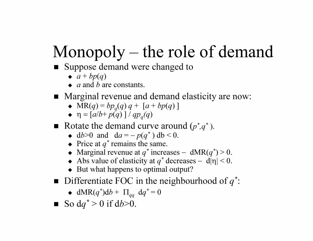
Monopoly – the role of demand� Suppose demand were changed to

� a + bp(q)� a and b are constants.

� Marginal revenue and demand elasticity are now: � MR(q) = bpq(q) q + [a + bp(q) ]� η = [a/b+ p(q) ] / qpq(q)

� Rotate the demand curve around (p*,q* ).� db>0 and da = − p(q* ) db < 0. � Price at q* remains the same.� Marginal revenue at q* increases − dMR(q*) > 0.� Abs value of elasticity at q* decreases − d|η| < 0.� But what happens to optimal output?

� Differentiate FOC in the neighbourhood of q*:

� dMR(q*)db + Πqq dq* = 0

� So dq* > 0 if db>0.

Monopoly – analysing the optimum

� Take the basic pricing rule

� p(q) = Cq(q)———1 + 1/η

� Use the definition of demand elasticity� p(q) ≥ Cq(q)

� p(q) > Cq(q) if |η| < ∞.

� “price > marginal cost”

� Clearly as |η| decreases:� output decreases.

� gap between price and marginal cost increases.

� What happens if |η| ≤ 1 (η ≥ −1)?

What is going on?

� To understand why there may be no solution

consider two examples.

� A firm in a competitive market: η = −∞

� p(q) =p

� A monopoly with inelastic demand: η = −½

� p(q) = aq−2

� Same quadratic cost structure for both:

� C(q) = c0 + c

1q + c

2q2

� Examine the behaviour of Π(q) .

Profit in the two examples

-200

0

200

400

600

800

1000

20 40 60 80 100

q

Π

q*

�Π in competitive example

η = −∞

�Π in monopoly example

nn

η = −½

�Optimum in competitive

example

�No optimum in monopoly

example

There’s a

discontinuity

here

The result of simple market power

� There's no supply curve:� For competitive firm market price is sufficient

to determine output.� Here output depends on shape of market

demand curve.� Price is artificially high:

� Price is above marginal cost� Price/MC gap is larger if demand is inelastic

� There may be no solution:� What if demand is very inelastic?

Overview...

Market supply

curve

Size of the

industry

Price-setting

Product variety

The Firm and the

Market

Modelling

“monopolistic

competition”

Market power and product

diversity� Each firm has a downward-sloping demand curve:

� Like the case of monopoly.

� Firms’ products may differ one from another.

� New firms can enter with new products.

� Diversity may depend on size of market.

� Introduces the concept of “monopolistic competition.”

� Follow the method competitive firm:

� Start with the analysis of a single firm.

� Entry of new firms competes away profits.

Monopolistic competition: 1

�For simplicity take linear

demand curve (AR)

�Marginal and average

costs

�Optimal output for single

firm

output

of firm

MC AC

MR

AR

p

q1

Π1

�The derived MR curve

�Price and profits

� outcome is

effectively the

same as for

monopoly.

Monopolistic competition: 2

output

of firm

p

q1

Zero

Profits

Review

� Individual supply curves are discontinuous: a problem for market equilibrium?

� A large-numbers argument may help.

� The size of the industry can be determined by a simple “entry” model

� With monopoly equilibrium conditions depend on demand elasticity

� Monopoly + entry model yield monopolistic competition.

Review

Review

Review

Review

Review

What next?

� We could move on to more complex issues

of industrial organisation.

� Or apply the insights from the firm to the

consumer.