First use of a HyViSI H4RG for astronomical observations

Lance M. Simmsa, Donald F. Figerb, Brandon J. Hanoldb, Daniel J. Kerrb, D. Kirk Gilmorea,

Steven M. Kahna, J. Anthony Tysonc

aStanford Linear Accelerator Center, Menlo Park, CA, 94025 USA;bRochester Imaging Detector Laboratory, Rochester, NY 14623 USA;

cDepartment of Physics, University of California, Davis, CA 95616 USA

ABSTRACT

We present the first astronomical results from a 4K2 Hybrid Visible Silicon PIN array detector (HyViSI) read outwith the Teledyne Scientific and Imaging SIDECAR ASIC. These results include observations of astronomicalstandards and photometric measurements using the 2.1m KPNO telescope. We also report results from a testprogram in the Rochester Imaging Detector Laboratory (RIDL), including: read noise, dark current, linearity,gain, well depth, quantum efficiency, and substrate voltage effects. Lastly, we highlight results from operation ofthe detector in window read out mode and discuss its potential role for focusing, image correction, and use as atelescope guide camera.

Keywords: H4RG, HyViSI Pin Array, SIDECAR ASIC

1. INTRODUCTION

The Hybrid Visible Silicon (HyViSI) H4RG is a hybrid CMOS (Complimentary Metal-Oxide-Semiconductor)4K×4K optical imager produced by Teledyne Scientic and Imaging (TIS). It consists of an H4RG multiplexerthat acts as a Readout Integrated Circuit (ROIC) and a 100 µm-thick layer of high purity bulk silicon that servesas the photo-detector. The two are sandwiched together, or hybridized, via indium bump bonds at the surface ofeach 10 µm × 10 µm pixel. On the ROIC side, the pixel consists of addressing, resetting, and readout circuitryand on the silicon side the unit cell contains a photodiode that collects photocharge at the site of a p+ implant.A high voltage source is attached to the illuminated side of the silicon layer in order to fully deplete the bulkof charge carriers. This provides a large depletion region for long wavelength photons to promote electrons intothe conduction band and inhibits the lateral diffusion of charge that tends to degrade the point spread function(PSF).

The hybrid CMOS architecture of the HyViSI H4RG and other hybrid CMOS sensors offers many of theadvantages of conventional CMOS devices and leaves behind some of the drawbacks of CCDs and non-hybridCMOS devices. As with most CMOS devices, operation of the H4RG sensor consumes very low power (operatedat 3.3V and lower) and enables on-chip integration of analog and digital circuitry.1 The CMOS architecture alsoeliminates the need to shift charge toward an output by allowing non-destructive, random access to the pixels;only one pixel-based charge-to-voltage conversion is necessary. Since any pixel can be accessed independentlyof the others, CMOS detectors do not suffer from charge transfer inefficiency (CTE) due to radiation damage,where a charge trap in one pixel can affect all of the ones following it in its row. The random access also allowsa sub-region of the detector to be read out continuously at fast rates, allowing for photometric measurements ofbright and/or rapidly-varying sources.

The 100 µm layer of silicon photodiodes atop the ROIC overcomes the problems of small fill-factor andinefficient charge collection associated with monolithic CMOS sensors.2 It offers nearly 100% fill factor andwhen fully depleted, the layer provides good quantum efficiency from the ultraviolet to 1.15 µm at the cutoff ofsilicon. As in the case of fully depleted thick CCDs, this large depletion region also provides a greater interactiondepth for high energy particles from cosmic rays and radioactive decay that result in wandering tracks and lossof imaging pixels.3 However, the non-destructive readout scheme implemented in CMOS devices offers a keyadvantage over the destructive one used in a CCD. The non-destructive reads allow up-the-ramp sampling that,in addition to lowering the read noise by sampling the voltages of each pixel multiple times during an integration,provides robust cosmic ray rejection with only one exposure. This is in contrast to CCDs, where typically two

or more exposures of the same length of time are required. The tradeoff is in the larger data volume associatedwith multiple up-the-ramp samples. If Bp is the number of bytes per pixel associated with the data, two CCDexposures with X × Y pixels will yield 2X ∗ Y ∗ Bp bytes while one CMOS up-the-ramp exposure with N readswill yield N ∗ X ∗ Y ∗ Bp bytes. Typically, 5 or more reads are required to reject cosmic rays with confidence.

The H4RG is a new device and only a small number of prototypes have been manufactured. One of them,H4RG-10-007, was purchased by the Large Synoptic Survey Telescope Corporation (LSST Corp.) and loaned tous at the Rochester Imaging Detector Laboratory for testing and characterization. The detector was read outby a TIS SIDECAR ASIC chip that provided an exceptional amount of functionality in a very small volume aswell as Generation III electronics from Astronomical Research Cameras (ARC).

In the following sections of this paper, we present pixel characterization and laboratory measurements ofdark current, read noise, electron conversion gain, well depth, linearity, and quantum efficiency for the HyViSIH4RG. We compare these results to those from other Si PIN devices. We then describe the process of reducingthe data taken at the telescope and show the results from relative photometry of standard stars and the M13globular cluster. Lastly, we discuss the data collected in window mode and use it to illustrate the potential ofthe H4RG as a detector for telescope focusing, image correction, and guiding.

2. LABORATORY TESTING

The goal of our lab testing program is to characterize Si PIN array technology for use in astronomical applications,with an emphasis on tests of the H4RG-10-007 device. Our testing follows a similar program used to evaluateJWST detectors.4 The testing yields measurements of the most relevant properties, i.e. gain, read noise, darkcurrent, linearity, etc., over a wide range of operational variations, i.e. temperature, read mode, and post-processing electronics architecture. The testing was performed in the Rochester Imaging Detector Laboratory(RIDL) within the Center for Imaging Science at Rochester Institute of Technology. The RIDL is a new facilitydedicated to the development of detector technologies for multi-disciplinary applications.

2.1 RIDL System

The RIDL system (see Figure 1) consists of software and hardware based on a system used to characterize infraredand optical detectors for space- and ground-based applications.5 The modular architecture of the system allowsfor rapid acquisition and reduction of large datasets over a broad range of experimental conditions. Minimaleffort is required to change between different detectors and different types of detectors. The system can betransported for operation on a telescope.

The system includes a 16 inch diameter dewar (Universal Cryogenics, Tucson, AZ) with a 110 mm diameterCaF2 window, two cryogenic filter wheels, and a detector enclosure. The system is cooled with a two-stagecooler (CTI Model 1050, Brooks Automation, Chelmsford, MA), and the detector is thermally stabilized witha 10-channel temperature controller (Lakeshore Cryotronics, Westerville, OH). The detector enclosure providesthermal and electrical feedthroughs, an entrance window, and an otherwise light-tight cavity for the detector. Thefilter wheels can accommodate eight filters and/or radiation sources. We use two sets of readout electronics: 1)the Generation III electronics from Astronomical Research Cameras, Inc. (San Diego, CA), and 2) the SIDECARASIC from Teledyne Scientific & Imaging, LLC (Thousand Oaks, CA). We used a variety of programmable gainsto obtain data and 5 us pixel time for the ARC electronics and 10 us pixel time for the SIDECAR.

2.2 Electronic Gain/Conversion Gain

There are a number of electrical gain stages in the signal path, and they collectively produce a net conversiongain, Gnet, in units of e−/ADU:

Gnet = Gpixel ∗ GUC ∗ GOUT ∗ GAMP ∗ GA/D (1)

The pixel gain, Gpixel (e−/V), represents the voltage change per unit charge, also known as the inverse ofthe capacitance. It is linear over small signal ranges but becomes nonlinear when the pixel is near capacity. Thedetector readout has two source follower FETs between each pixel and the output pad. One is in each unit cell,

Figure 1. RIDL system. An orange dewar houses two filter wheels and a detector enclosure. A helium cryo-cooler coolsthe system. The picture shows an integrating sphere and monochromator near the front of the dewar. Post-processingelectronics are mounted on a plate attached to the top side of the dewar. Off camera are three computers (two four-wayand one eight-way CPU) with 4 GB, 12 GB, and 16 GB of RAM and 12 TB of RAID5 storage.

and it induces a gain of GUC (V/V). The other, the output FET, introduces a similar gain, referred to as GOUT

(V/V). The processing electronics have stages to amplify the signal, GAMP (V/V). Finally, GA/D (V/ADU),represents the conversion between volts and analog to digital units (ADUs). We have developed procedures tomeasure each of these gains.

First, we establish GA/D by dividing the range of ADUs measured as a response to a well-characterizedsawtooth pattern by the voltage range of that sawtooth. This measurement is done without the amplifier gainstage in the circuit. Next, we measure GAMP by repeating the sawtooth experiment with the gain stage inthe circuit. We find GUC by bypassing the output FET and measuring the response to a varying reset voltageprogrammed onto the gate of the pixel FET. Next, we repeat the reset experiment with the output FET inthe circuit in order to measure GOUT . Finally, Gpixel is inferred by inverting the equation above and usingthe full conversion gain from our Fe55 experiment. In this experiment, an Fe55 source is placed an inch abovethe detector and we operate the device in photon-counting mode. The conversion gain is simply 1620 electronsdivided by the peak of the photon hit distribution. Table 1 summarizes the gain measurements for the H4RG-10-007 detector and the ARC electronics. Note that the measurements are given for two different amplifier gains.Figure 2 shows a photon counting image and histogram produced by this experiment.

Table 1. Measured gains using the ARC electronics and the H4RG-10-007 Si PIN detector

H4RG ARC SFE

GAMP Fe55 peak Conversion GA/D Unit Cell GUC ∗ GOUT 1/Gpixel Unit Cell

Gain Gain Capacitance

(V/V) (ADU) (e−/ADU) (µV /ADU) (µV /ADU) (V/V) (µV /e−) (fF)

1.81 699.2 2.32 42.97 58.411 0.736 25.21 6.347

6.62 2590 0.63 11.08 15.292 0.725 24.45 6.544

Figure 2. Histogram of signal generated by x-ray photons from Fe55. The photons each liberate 1620 electrons; theconversion gain 1620/647.9=2.5 electrons/ADU.

2.3 Pixel Characterization

We have identified several different types of pixels on the H4RG that cannot be used to accurately estimateluminance. They are categorized as dead, hot, and open pixels. These pixels are masked and not used in theanalysis of our observational data. All of the other pixels on the detector are of suitable quality to be used inthe observational data analysis.

2.3.1 Dead Pixels

The first type of unusable pixels are dead pixels that do not integrate charge, whether exposed to light or not.Most of them are railed at the high end of the detector voltage range, suggesting they are shorted to one of thehigh bias voltages. These pixels are easy to detect since they do not show an increase in signal over time. Inorder to find them, we took differences between a read r and the zeroth read r = 0, in the flat field and darkimages and flagged pixels that had a difference in signal, I, below a certain threshold T . i.e.

I(x, y, r + 1) − I(x, y, 0) < T, (2)

for all r. T depends on the gain of the pre-amps in the SIDECAR ASIC, but is typically set at 3 × Nr, whereNr is the read noise of the detector at that gain.

In all, there are 6341 of these pixels on the detector, representing 0.038% of the total number of pixels. Thisnumber includes an entire row of 4096 pixels that is presumably a bad line in the ROIC.

2.3.2 Hot Pixels

The hot pixels are found by (1) looking for very high pixel signal slopes, ∆I/∆t, and (2) looking for pixels thathave a value of I greater than 75% of the full A/D range in the zeroth read. In the latter case, the dark current isso extreme that the pixel voltage reaches the upper rail almost immediately after reset, and its slope is flattenedbefore the zeroth read. There are a total of 210,063 (1.252%) pixels that meet this criteria.

2.3.3 Open Pixels

The open pixels are pixels that have a value that falls significantly below that of their nearest neighbors inwell-illuminated images. I.e.

I(x, y, r) � I(x ± 1, y ± 1, r). (3)

These pixels are presumed to be open in the sense that the indium bump bond does not connect the siliconsubstrate to the ROIC. Their spatial distribution over the detector is not uniform over the detector, and it hasbeen mapped to a set of suspected opens by Teledyne. There are a total of 76,959 open pixels on the detector,representing 0.459% of the total population.

Figure 3 shows isolated black squares and black squares surrounded by neighbors with enhanced signal. Weassociate the former with hot pixels. We have verified that their signal quickly reaches saturation such that theyappear dark in a difference image. The black pixels with bright neighbors are open pixels, i.e. pixels with poorbump bond interconnects.

While the open pixels appear to be dead in the stretch shown in the figure, they do have increasing signalversus read number, but the slope does not depend on the presence of light. Their neighbors have extraordinarilylarge signal. In a flat field image, the cumulative augmented signal in the eight nearest neighbors to an open

Table 2. Bad pixels

Pixel Type Number Fraction Characteristics

Dead 6341 0.038% no signal accumulation

Hot 210,063 1.252% rapid signal accumulation

Open 76,959 0.459% nearest neighbors show rapid accumulation

Figure 3. Difference image of portion of H4RG-10-007 array under flat field illumination at 1000 nm. Notice that thereare two populations of dark pixels. One is surrounded by neighbors with normal response and another is surrounded bypixels with elevated apparent response. The former are identified as hot pixels which have a difference near zero and thelatter are identified as open pixels.

pixel is 70% of the signal that should have been in the open pixel. Interestingly, 30% of the signal that shouldbe in the open pixel is unaccounted for. Perhaps the open pixels have very high impedance connections to thereadout circuit so that they integrate some charge; however, most of the charge generated in the bulk materialof the pixel migrates to neighbors. (Note that by just looking at the figure, one might propose that the ”open”pixels are actually very hot pixels that difference to zero in the difference image in the figure. In this case, onemight suggest that the neighbors have enhanced signal because of interpixel capacitance. This cannot be true,because we have verified that the open pixels do indeed have low counts in individual reads - they are neversaturated).

2.4 Reference Pixels and Channels

The H4RG ROIC contains two types of reference pixels. The first type is identical to science pixels, except thebackside has been blackened to prevent light from entering the substrate. The second type consists of capacitorswith a capacitance Cpix similar to the detector capacitance and is the same as in previous HxRG designs. Inpractice, we found that the two different types of reference pixels have dramatically different behavior. Figure4 shows that the blackened type has dark current that is similar to that in nearby science pixels. On the otherhand, the capacitor type does not integrate dark charge. Depending on the goal, one might choose to use eitherpixel type. For instance, if one wants to remove common mode interference, then the capacitor type might bethe most useful. On the other hand, one could use the blackened type to remove this interference and also someportion of the dark current. For characterizing the detector technology, we found it useful to not use referencepixel subtraction. We saw no noise penalty in doing this.

2.5 Well Depth and Linearity

We measure the well depth and linearity by exposing the detector to a flat illumiination source and obtaining aramp with many reads through the saturation level. Figure 5 shows that the H4RG-10-007 detector saturates atabout 55 ke−, and that the saturation level varies by about 2%. Figure 6 shows the saturated image; note thepopulation of bad (open) pixels that do not respond to light. The linearity plot, in the bottom panel of Figure5 shows the average of normalized slopes for all of the pixels on the detector at a particular ADU value. Thenormalization is with respect to the slope between the first and zeroth read of the ramp for each pixel. The figure

Figure 4. Behavior of reference pixels. The capacitor-type reference pixels do not integrate dark current charge (upperleft) as do the science pixels (upper right). The blackened reference pixels do integrate dark current charge (lower left),similar to what is seen for a science pixel in the same image (lower right).

shows that the detector is linear to within a few percent over 90% of its well range, and that the non-linearityis well-fit by a second order polynomial, to within a few tenths of a percent over most of the well range. Thisnon-linearity is reproducible to within a few tenths of a percent.

Figure 5. Histogram of well capacity (top) and linearity versus fluence (bottom).

Figure 6. Saturated image. The numbers on the color scale are in ADU and can be multiplied by 2.5 to convert toelectrons. The dark pixels correspond to the open pixels and have low quantum efficiency. The electronics for outputcolumn 8 (from the left) had intermittent connection that produces artifacts not related to the detector.

2.6 Dark Current

We measure dark current as a function of temperature for each pixel by fitting a linear slope to the increasingsignal values in a sequence of non-destructive reads ”up-the-ramp.” Figure 7 shows the median dark currentversus temperature for the H4RG-10-007 device. Figure 8 shows a similar plot for the devices we have measured,where the dark current has been converted into a density to account for the 10 micron pixel size of the H4RG-10-007 device and the 18 micron pixel size of the other devices. Note that the dark current density for theH4RG-10-007 device is relatively high and its dependence on temperature is relatively weak.

Figure 7. Dark current versus temperature for H4RG-10-007.

Figure 8. Dark current versus temperature for H4RG-10-007 along with several other HxRG detectors.

Figure 9. Curves of raw signal versus read number for a single pixel with increasing VRESET toward the top. The topfew curves are overlapping. The apparent dark current is going down with increasing VRESET, to the point where it isnon-existent for the highest VRESETs.

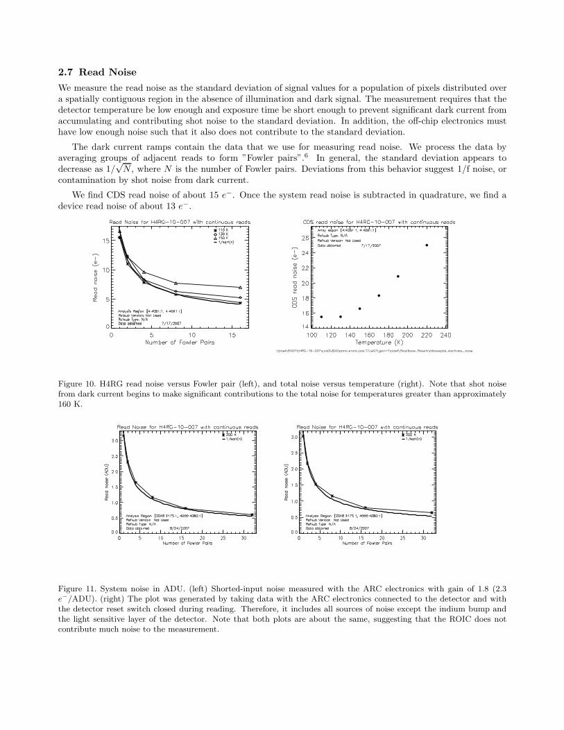
2.7 Read Noise

We measure the read noise as the standard deviation of signal values for a population of pixels distributed overa spatially contiguous region in the absence of illumination and dark signal. The measurement requires that thedetector temperature be low enough and exposure time be short enough to prevent significant dark current fromaccumulating and contributing shot noise to the standard deviation. In addition, the off-chip electronics musthave low enough noise such that it also does not contribute to the standard deviation.

The dark current ramps contain the data that we use for measuring read noise. We process the data byaveraging groups of adjacent reads to form ”Fowler pairs”.6 In general, the standard deviation appears todecrease as 1/

√N , where N is the number of Fowler pairs. Deviations from this behavior suggest 1/f noise, or

contamination by shot noise from dark current.

We find CDS read noise of about 15 e−. Once the system read noise is subtracted in quadrature, we find adevice read noise of about 13 e−.

Figure 10. H4RG read noise versus Fowler pair (left), and total noise versus temperature (right). Note that shot noisefrom dark current begins to make significant contributions to the total noise for temperatures greater than approximately160 K.

Figure 11. System noise in ADU. (left) Shorted-input noise measured with the ARC electronics with gain of 1.8 (2.3e−/ADU). (right) The plot was generated by taking data with the ARC electronics connected to the detector and withthe detector reset switch closed during reading. Therefore, it includes all sources of noise except the indium bump andthe light sensitive layer of the detector. Note that both plots are about the same, suggesting that the ROIC does notcontribute much noise to the measurement.

2.8 Detective Quantum Efficiency (DQE)

DQE is the realized S/N compared to that of an ideal detector. It is often measured in the background-limitedcase so that it is most closely related to the photon capture process in the bulk material of the detector, asopposed to being related to read noise effects in the post-capture electronics. DQE can vary with wavelength,temperature, and individual pixel properties, to name a few examples. In the RIDL experiment, we illuminatethe detector with a monochromatic flat field produced by an integrating sphere and monochromator. The lightis monitored by a calibrated silicon photodiode located at a port on the integrating sphere. In future testing, asimilar calibrated diode will be placed at the location of the detector in order to transfer the flux measured atthe integrating sphere to the focal plane. Once this wavelength-dependent calibration is made, the detector willthen be placed at the focal plane and the experiment repeated.

Figure 12. H4RG-10-007 relative QE versus wavelength (left) and H2RG-003 relative QE versus temperature (right) nearthe long wavelength cutoff. The results show that QE increases with temperature and are consistent with a silicon detectorhaving 100 um thickness.

Figure 13. Fringing seen in monochromatic flat field images near 1 um obtained with the H2RG-003 device (left). Thefringing indicates thickness variation of a few microns. Fringing for the H4RG-10-007 device (right). The columnarstriping is an artifact of electronic readout offsets and is not a QE variation of the detector.

2.9 Pixel Behavior Vs. VSUB

VSUB sets the backside contact voltage and, along with DSUB, defines the electric field strength in the bulk.Figure 15 shows the behavior of the median dark current across the array for three values of VSUB: 0 Volts, 5Volts, and 30 Volts. In the first case, photogenerated charge in the bulk is under no force to migrate toward thecharge collection node. Because of this, little charge is integrated. Note, though, that there are still many hotpixels, suggesting that charge generation in hot pixels is localized near the charge collection node. At VSUB=5Volts, charge integrates on the collecting node, but there is significant lateral diffusion. This is to be expected,as the electric field is not strong enough to provide full depletion. At VSUB=30 Volts, the effective point spreadfunction is much tighter.

Figure 14. Signal versus read number for open (upper) and hot pixels (lower) under no voltage (left) and 30 Volt (right)levels for VSUB. The bold lines refer to a central pixel, and the remaining eight lines are for the nearest neighbors. Bothopen and hot pixels have constant behavior versus VSUB. At high VSUB, charge generated in the open pixel migratesto neighbors. Note that one of the open pixel neighbors is hot, and one of the hot pixel neighbors only becomes hot asvoltage is applied to VSUB.

Figure 15. Median dark current and images versus VSUB (0 Volts, top, 5 Volts, middle, 30 Volts, bottom). Hot pixelsappear extended at VSUB=5 Volts because the bulk is not fully depleted.

2.10 Window Mode

We exercised window mode using multiple sized windows. Figure 16 shows signal versus time extracted from awindow of a dark image. The estimated CDS noise is 15 electrons, and the power is white. The noise can beaveraged down as 1/root(n), where n is the number of reads.

Figure 16. Signal (ADU) versus read number for a pixel in a 10x10 window centered on pixel 505,505 of the H4RG-10-007.The gain is 1 electron per ADU, and the CDS read noise is 15 electrons. The noise is white, although the signal appearsto increase slightly just after reset, akin to the reset anomaly typically seen in hybrid devices.

Figure 17. A photograph of the RIDL dewar mounted to the Kitt Peak 2.1m telescope.

3. OBSERVATIONS

We observed on the 2.1m telescope at the KPNO observatory in Tucson, Arizona (110◦ 58′ 0′′ W, 32◦ 13′ 0′′ N)during the nights of 4/25/2007-5/1/2007. A picture of the RIDL dewar and electronics mounted to the telescopeis shown in Figure 17. With an f7.6 beam and 10 micron pixels spanning a 40.96×40.96mm array, the plate scalewas approximately 0.126′′ per pixel and the field of view was 8′×8′. The H4RG detector was housed inside theRIDL dewar and positioned behind a filter wheel with six positions controlled by Phytron motors. Two of thepositions were left open, one was a blank that prevented light from reaching the detector, and the other threewere occupied by g,i, and y filters, described in Table 3. To accommodate the RIDL dewar, the telescope guidercamera was removed from the telescope. The telescope was set to track at the sidereal rate and a rotator wasused to correct for rotations of the field of view.

During our observations at the telescope, a stray signal was present somewhere in the electronics and thisgave rise to ”pseudo-random” noise that appeared in our images. The source of the signal was traced to a USB tooptical fiber converter device, but attempts to remove it proved futile. We refer to it as ”pseudo-random” becausethe oscillations in the electrical signal were not in sync with the reading of the electronics and so it appeareddifferent in each image, but the temporal power spectrum was very repeatable throughout our observations. Atypical power spectrum and signals from each of the nights are shown in figure 18 below. There is very littlepower at frequencies above 40 Hz.

Since one of the 32 inputs on the SIDECAR ASIC was not sensitive to the analog signal coming from the0th output of the H4RG, we chose to use this entire channel in addition to the reference columns on the left andright side of the detector to attempt removal of the common mode noise. This task has proven difficult, however,since the scale of the fluctuations seems to vary over the detector. Unfortunately, the signature is still apparentin our science images.

Table 3. Filter Characteristics

Filter Name Peak Cuton Cutoff Transmission

(nm) (nm) (nm) (%)

g 476 401.22 557.87 96.39

i 742 667.61 815.77 96.14

y 1003 970.54 1036.01 86.28

Figure 18. (Left) Average power spectrum of all 128 channels corresponding to output 0 of the H4RG detector. (Right)Deviation of the median of each row in Channel 0 from the mean of Channel 0.

Our observations consisted of full frame exposures – ones in which we clocked through every pixel in thedetector one or more times – and window mode exposures – ones in which we clocked through only the pixelsin a sub-region of the detector one or more times. The full-frame mode is well suited for long exposures of faintobjects and the window mode is more appropriate for high speed photometric measurements or telescope guiding.Each will be discussed in turn.

3.1 Full Frame Mode

A diagram that illustrates a full frame ramp sequence is shown in figure 19.

Figure 19. (Left) An Illustration of the ramp sequence, courtesy of Markus Loose. The number of resets, drops, groups,and reads are programmable in software, allowing control over the expousure time. (Right) An oscilloscope trace of severalclock lines on the SIDECAR ASIC. The delay time trs is visible.

The ramp consists of a series of N frames, the basic unit in which the entire array of pixels is clockedthrough. The clocking scheme is similar to the one employed in CCDs, with a fast direction along the rowscontrolled by a horizontal clock (HCLK) and a slow direction along the columns controlled by a vertical clock

(VCLK). The duration tf of the frame is determined by the pixel time tp, which corresponds to the time betweenedges of the HCLK signal configurable on the ASIC, and the number of outputs No used on the H4RG, eachof which is paired with an input on the SIDECAR ASIC. It is roughly tf = tp ∗ 4096 ∗ 4096/No + 4096 ∗ trs,where trs is a time associated with moving to the next row of 4096/N0 pixels in the array. tf is also the timebetween reading a pixel in one frame and reading that same pixel again in the following frame. The SIDECARASIC we used had a maximum of 36 inputs, so we chose No = 32, and we used a 10 µs pixel time, givingtf = 5.24288s+ 4096 ∗ trs. Eventually, we implemented a counter on the SIDECAR that allowed us to preciselymeasure a time of tf = 5.453s and trs = 52us. This was also verfied on an oscilloscope, the trace of which isshown in Figure 19.

The illustration shows three different types of frames : reset frames, drop frames and read frames. Duringthe reset frames, the array is clocked so that the gate of the reset FET in the ROIC pixel is enabled and thepixel is held at the voltage VRESET supplied by the SIDECAR ASIC. This allows the charge on the capacitivenode in the silicon to dissipate so that it is ready for a subsequent integration. In the read frames, the columnselect and row enable signals for all of the pixels are enabled in turn, bringing the voltage at a pixel to itscorresponding output FET. This voltage is converted to a digital number and sent out to the Data AcquisitionSystem (DAQ) for recording. The unique feature of the drop frames is that no data is output from the SIDECARto the computer. This allows the user to take a very long exposure without dealing with overwhelming amountsof data. It should be mentioned that data from the reset frames can be output to the external DAQ and thepixels can be clocked during the drop frames by writing to registers on the SIDECAR ASIC.

In a fashion similar to the scheme used in the NICMOS and JWST specifications,7 we refer to a ramp havinga cadence of Nrs reset frames, Nd drop frames, Ng group frames, and Nrd read frames, as a Nrs-Nrd-Nd-Ng

ramp. Such a ramp has a total of Ng ×Nrd data frames. With these definitions, the exposure time of a ramp infull frame is given by

te = Ng ∗ (Nd + Nrd) ∗ tf , (4)

with tf being the frame time given above. To avoid confusion in the following sections, we will use this syntaxand reserve the terms ramp or exposure for such a sequence. We will use the terms read or frame to describea read frame in these ramps. And the term image will be used to refer to the data produced after reduction ofthese ramps, which is described in the next section.

Figure 20. An illustration showing the sequencing and times (described in text) involved with window mode. The linelabeled trs at top shows the path taken in single window mode and the line labeled tws line shows that taken in multiple

window mode when N = 2 windows are used.

3.2 Window Mode

The H4RG contains a serial register that can be configured to allow random access to a contiguous X×Y subsetof pixels, or window, through one output of the detector. X and Y , the number of columns and rows in thewindow, respectively, must be greater than 1 pixel and less than 1024 pixels. Programming the addresses of thewindow limits, Xstart, Xstop, Ystart, and Ystop, can be done on the fly. This allows multiple windowed regions ofthe detector to be read out in a ping-pong like fashion and also the possibility of feedback control loops in whichthe window coordinates are continually adjusted to track an object. We used the window mode functionalityfor three purposes: (1) to focus the telescope in real time, (2) to observe objects that were suspected to varyon short timescales (< 1s), and (3) to collect data on absolute and differential image centroid motion across our8′× 8′ field of view.

Our basic unit in a window mode observing sequence is a correlated double sample in which we clockedthrough all X ∗Y pixels in a window 3 times, resetting each pixel once and then reading the pixel voltages twice.The clocking is similar to full frame mode, with the fast clocking along the rows and the slow clock along thecolumns. With a pixel time of tp, one row takes X ∗ tp seconds with an additional trs seconds of overhead inshifting to the next row. To complete all rows thus requires tw = Y ∗ (X ∗ tp + trs) seconds and this is the totaltime for a reset or a read in the window sequence. An effective exposure time for a CDS in window mode is givenby

te = 2tw + 2trs, (5)

the time between the reset of a pixel and sampling it in the second read. For our observations, we used a pixeltime of tp = 10µs and mimimized the overhead to attain trs = 18µs. tp can be be decreased in order to decreasethe time to complete one CDS sequence and up the sampling rate with a penalty in noise.

After a CDS sequence, either another CDS is repeated on the same window or the serial register is pro-grammed with a new set of window coordinates. We refer to the former as single window mode and the latter asmultiple window mode. With the microcode used on the SIDECAR ASIC, the operation of writing new windowcoordinates for Xstart, Xstop, Ystart, and Ystop takes tws = 150µs; adjusting only two of these four would take ∼75µs. A diagram showing the times associated with window mode is shown in Figure 20. It should be apparentfrom the diagram that if N windows are used in multiple window mode, the time it takes to complete a full cycle

and return to the first window is given by:

tmwc = 3Ntw + 2Ntrs + Ntws (6)

And if single window mode is used this time becomes:

tswc = 3(tw + trs) (7)

It is also important to know the time between exposures in different windows for the purposes of measuringtemporal correlations. In multiple window mode, the time it takes between a CDS in window n and a CDS inwindow m is given by

tnw = 3(m − n)tw + 2(m − n)trs + (m − n)tws (8)

The full cycle is repeated M times in one full observing sequence, giving a total time of M ∗ tmwc in multiple

window mode and M ∗ tswc in single window mode.

While taking window data in both single and mutliple modes at the telescope, the bias subtracted imageswere displayed on screen via a graphical user interface, and the contrast of signal to background was quiteencouraging. However, due to a software error, the first read in our multiple window exposures were not saved;only the zeroth read was. This makes the contrast in the saved data of much poorer quality. We will presentresults from the single window mode data as an indication of the signal to noise ratio that should be achievablefor both modes. And despite the noisy nature of the multiple window mode data, we will use it to highlightthe potential of the H4RG to track centroid motion across a large field of view by considering only very brightobjects for which the zeroth read still provides an ample signal to noise ratio.

4. DATA REDUCTION

4.1 Full Frame Mode

Each night before we observed we took a set of 1−0−2−1 flat-field ramps through each filter and each morninga set of dark ramps that matched the cadence of the ramps that we had used in our exposures during that night.For each of these ramps, the first read (bias) was subtracted to eliminate kTC noise and a median filter wasapplied to each set to reject cosmic rays and outliers. This operation yielded one median flat-field ramp withpixel values I l

flat(x, y, r), for each filter l and one median dark ramp with pixel values Idark(x, y, r) for eachcadence.

4.1.1 Dark Subtraction

¿From each exposure of the sky through a given filter we subtracted a median dark ramp of the same cadencefor each pixel, i.e Iobj(x, y, r) = Ilum(x, y, r) − Idark(x, y, r), where Ilum is the pixel value from the illuminatedimage. The resulting frames in this ramp should, in theory, have pixel values Iobj that correspond to luminancefrom the source being observed.

4.1.2 Slope Fitting

Although the dark current signal Idark and illuminated signal Ilum on H4RG-10-007 appear to be nonlinear withrespect to time, the difference Ilum − Idark shows good linearity over a large fraction of the full well. Figure 21,generated from the median of a set of 30 1-0-30-1 y band ramps in which the detector was uniformly illuminated,is indicative of this. It shows a plot of the average of the normalized slopes mn = (Iobj(x, y, r)−Iobj(x, y, 0))/t(r)at a given ADU value, Ilum(x, y, r), vs. ADU value, with t(r) being the time at read r. The normalization ismade on a per pixel basis by finding the slope, mo = (Iobj(x, y, rmax) − Iobj(x, y, rmin))/(t(rmax) − t(rmin)),

that minimizes the quantity Err =∑N

1 abs[Iobj(r) − (mo ∗ t(r) − b0)] for all values of t before Iobj reaches itsmaximum value in the ramp. rmax and rmin are different for different pixels, but average values are rmin = 5and rmax = 22. As indicated in the figure, on average the slope of each ramp deviates by less than 5% from mo

over 85% of the full ADU range. Nonlinear effects appear in the lowest 8.25% ADU values and the uppermost6.4% ADU values. A more proper treatment would be to obtain lower and upper limits like this for each pixelby collecting data at many different levels of illumination and exposure times. We plan on doing this in a futureexperiment.

Figure 21. (Left) Linearity of the H4RG on the night of 4/27/07 with a gain of 1. (Right) A 650x550 pixel cut-out froma false-color image of M57 made by combining the reduced images from the g and i filters.

The slope mo is useful for determining ADU values Iminlum and Imax

lum between which the ramps are most linear.However, mo does not provide the best estimate of the true slope within these limits for each pixel since it isconstrained to contain two points in the ramp. In order to find the slope that minimizes the error for the pointsin the linear regime, i.e. where Ilum lies between Imin

lum and Imaxlum , we fit a line to the corresponding values of Iobj

using the technique described in Numerical Recipes.8 Namely, for a pixel that has Nrd = rmax − rmin values ofIlum(r) between reads rmin and rmax, and corresponding dark subtracted values I(r) = Iobj(r),

b =

∑rmax

rmint(r)2

∑rmax

rminI(r) −

∑rmax

rmint(r)

∑rmax

rmint(r)I(r)

Nrd

∑rmax

rmint(r)2 −

(∑rmax

rmint(r)

)2 , m =Nrd

∑rmax

rmint(r)I(r) −

∑rmax

rmint(r)

∑rmax

rminI(r)

Nrd

∑rmax

rmint(r)2 −

(∑rmax

rmint(r)

)2 .

(9)b is an approximation to the bias offset in ADU, and m is the number of ADU/s attributed to the source ofillumination. It should be apparent that only the difference in times t(r) and t(r + 1) matters, so it suffices touse the average time for the rth read. With a slope obtained and the proper conversion gain in e−/ADU , m canbe converted to units of e−/s.

Bright objects will induce saturation very quickly, and in some cases there will be too few or no values ofIlum(r) in the linear regime. These cases require alternative approaches. If a pixel is saturated in the first read(the bias read is considered the zeroth read) and Ilum(0) < Imax

lum − 0.5IFRlum, where IFR

lum = Imaxlum − Imin

lum , the slopeis approximated by the CDS value m = (I(1) − I(0))/(t(1) − t(0)). And if a pixel is saturated in the first readand I(0) > Imax

lum − 0.5IFRlum, the best one can do is approximate the slope by m = I(0)/t(0).

Once a slope has been fit to the points in the linear regime, cosmic rays are detected as large deviations fromthe fit using the same method as the one in the NICMOS reduction code.9 In this method, the difference betweenthe data points and the fit is first computed as D(r) = I(r)− (b−mt(r)). Then the difference between adjacentpoints in this difference is taken, DD(r) = D(r)−D(r−1)) along with its standard deviation, σDD. Cosmic raysare flagged as points where DD(r) > TrσDD, where Tr is some threshold. For our H4RG data, Tr was typicallyset around 3. The idea behind this scheme is that the cosmic rays particles will release significantly more chargein the pixel over some small time interval then the integrating photocurrent and show up as a large negative topositive spike in Di. Using a separate σDD for each individual pixel seems to be quite effective and well suitedfor treating the variation in pixel sensitivity across the array. If a cosmic ray is detected in a read r = rcr latein the ramp, rcr > rmin + Nrd/2, then the slope is refit using points from r = rmin to r = rcr. If it is detectedearly in the ramp, rcr < rmin + Nrd/2, the slope is refit using points r = rcr to r = Nrd. If enough points are

Figure 22. (Left) A section of the cosmic ray image from a 15 read ramp. (Right) Signal vs. time for a pixel that hasbeen hit with a cosmic ray. The black dashed line is the high slope originally fit to the line and the red dashed line is thelower slope after the cosmic ray has been detected in the slope fitting algorithm.

left, another iteration of the cosmic ray detection sequence is performed. The number of points included in thefit is included as an extension to the image for purposes of error analysis.

An added benefit of the up the ramp sampling is that the energy deposited by a high energy particle canbe well approximated by examining the signal Ircr

− Ircr−1. These values are recorded and stored as a separateimage. They are potentially interesting for measuring the angular distributions, frequency, and morphology ofsuch events. An example is shown in Figure 22.

4.1.3 Flat Fielding

After every pixel has had a slope fit to it for the exposure, we are left with a 4096×4096 array of slopes, m(x, y),that we take to be the image. This image is divided by the normalized, bias-subtracted, first read I l

flat(x, y, 1)of the median flat-field through that same filter to correct for variation in pixel sensitivity.

4.1.4 Combining Dithers

For our full frame exposures, we used a dithering technique to provide a number of samples of each field. Thedither pattern was a 3x3 box where each telescope pointing was offset from the previous one by 20 ′′, or ∼160pixels. A full exposure was taken at each of these pointings, giving us 9 slopefitted images of the field in eachfilter.

The 9 slope images from each filter are aligned using several bright stars and combined into a mosaic. Tocombine the data from the 1-9 pixel values at a spatial location (x,y) in mosaic image coordinates, we used botha median filter and the mean of the pixels that were not flagged as bad or rejected as 3σ outliers. Using nineimages ensured that we had a minimum of three reasonable pixel values in nearly all cases (near the boundarieswas an exception), and it was found that the latter method yielded better results than the median filter as itreduces the noise by a factor of

√1−

√9. These mosaics are the images that we use for analysis in the following

sections.

4.2 Window Mode

We did not collect dark current data for our window mode exposures. This is problematic because the chargethat accumulates in a pixel due to dark current in a window mode exposure is different from that in a full frameexposure since the time between a reset and read of that pixel differs between the two. However, since the sourceswe observed in window mode were typically very bright, with a magnitude < 13, Ilum � Idark, we are still ableto estimate the signal due to the intensity of the source. In future observing runs, we plan to collect matchedsets of darks for all of our window mode exposures.

Because of the lack of dark data, the procedure for reducing the window mode data was to subtract the biasread (when available) and divide by the flat-field with matching filter for each CDS sequence. In single windowmode, this provides a datacube consisting of M X × Y images at times t = i ∗ tsw

c , where i = 0, 1, 2, ...M .In multiple window mode, it provides a datacube of M X × Y images for each of N windows, sampled att = i ∗ tmw

c + tnw, where i = 0, 1, 2, ...M and tnw is calculated from equation 8 using n = 0 and m = 0, 1, ...N asthe index of the window in the sequence of N windows.

5. PHOTOMETRY

To assess the potential of the H4RG as a photometric instrument, we measured instrumental magnitudes of wellisolated standard stars in the Landolt Equatorial Fields PG 1530 and SA 109 as well as stars in the crowdedfield of the M13 cluster. Photometric measurements of Landolt stars is well suited for testing the ability of thedetector to sense brightness differences within a particular wavelength passband as well as determining how wellit can be calibrated to obtain absolute magnitudes within that band. Crowded-field photometry of the starsin M13 is good for determining the spectral responsivity of the detector by comparing measurements throughseparate passbands since the relationship of color index vs. magnitude has been well studied in the cluster.

5.1 Aperture Photometry: Landolt Standards

Landolt Standard stars provide a good set of basis measurements for comparison as they have been repeatedlyobserved through different filter sets with different calibrated instruments. Unfortunately, these standards havebeen observed very frequently through UBVRI filters of the Johnson-Kron-Cousins system, but not through g,i,and y filters that are more closely matched to our set. It is possible, however, to make a transformation betweenpairs of filters in these two systems under the assumption that the variation of the spectral energy distributionE(λ) of the stars is sufficiently continuous over the intervals considered to allow a Taylor expansion in λ.

Such a tranformation is done, as in,10 by solving the following equations:

mH4RGl = MCAL

j Z − KX + CT × (MCALk − MCAL

j ), (10)

where MCALj is the reference magnitude in the filters j = V , I, and Y , mH4RG

l is the instrumental magnitudethat we measured through the filters l = g, i, and y, X is the airmass, K is the atmospheric extinction coefficient,CT is a color coefficient and MCAL

k − MCALj is the color defined by filter j and k = B, R, and H from the

reference measurements. Astronomers frequently use these equations in order to compare measurements madeat different telescopes and to calibrate for slight differences between filter sets. They are typically solved usinga population of several hundred standard stars. Due to limited time and data, we have only seven.

The transformations require a calculation of an average airmass over the duration of our exposures in eachfilter band. For this we used the algorithm suggested by Stetson11 : Xavg = (Xbeg + 4Xmid + Xend)/6, whereXbeg is the airmass at the beginning of the first exposure, Xmid is the airmass midway through the exposure(for us it was the fifth dither in the sequence) and Xend was the airmass at the end of the dither sequence. Theaverage airmasses through which we observed ranged from 1.12 to 1.26, so loss due to atmospheric extinctionwas not very significant.

Once the equations are solved, they can be used to predict the magnitudes we should expect to observe for g,i, and y filters at zero airmass based upon standard magnitudes in V , I, and Y and the corresponding colors. Thefitting coefficients and errors are shown in Table 5 and a plot that illustrates the goodness of the fit is shown inFigure 23. The errors in the fit are not unreasonable. They are similar to the ones found in the transformationsmade in the Sloan Digital Sky Survey.12 The error in g is substantially higher than it is in i and y. This maybe attributed to a number of factors including observing conditions, wavelength dependent lateral diffusion inthe detector, and nonlinearity. The exact reason for the large discrepancy is still being investigated. However,the data and the fit indicate that the H4RG is capable of doing absolute photometry. In future observations weplan to obtain a larger sample of measurements on standard stars in order to obtain the relative error in thephotometry.

Table 4. Landolt Star Magnitudes. Our measured magnitudes are denoted by lowercase m. M are catalouged magnitudes;+ are taken from Landolt (1973)13 , � are taken from Landolt (1992),14 and ? from Gullixson (1995).15 All MY are fromPersson (2002).16

Star MCALY ∆MCAL

Y MCALY Error MCAL

Y − MCALH mH4RG

y ∆mH4RGy mH4RG

y Error

109-956 12.516 0.000 0.029 1.038 15.362 0.000 0.001

109-954 10.254 2.262 0.028 1.064 13.079 2.283 0.001

109-949 11.384 1.132 0.029 0.595 14.250 1.112 0.001

MCALV ∆MCAL

V MCALV Error MCAL

B − MCALV mH4RG

g ∆mH4RGg mH4RG

g Error

109-959 ? 12.790 0.000 0.029 0.780 12.404 0.000 0.003

109-956 � 14.639 -1.849 0.011 1.283 14.407 -2.003 0.009

109-954 � 12.436 0.354 0.009 1.296 12.187 0.217 0.003

109-949 � 12.828 -0.038 0.006 0.806 12.408 -0.004 0.002

1530-057 � 14.21 0.000 0.000 0.151 12.756 0.000 0.003

1530-057A� 13.71 0.500 0.000 0.829 12.514 0.242 0.003

1530-057B� 12.84 1.37 0.000 0.745 11.595 1.161 0.002

MCALI ∆MCAL

I MCALI Error MCAL

R − MCALI mH4RG

i ∆mH4RGi mH4RG

i Error

109-959 + 11.572 0.000 0.009 0.671 12.197 0.000 0.003

109-956 � 13.114 -1.542 0.016 0.743 13.886 -1.689 0.007

109-954 � 10.940 0.632 0.003 0.731 11.391 0.806 0.002

109-949 � 11.708 -0.136 0.003 0.517 12.422 -0.225 0.003

1530-057 � 14.011 0.000 0.000 0.036 12.967 0.000 0.003

1530-057A� 12.842 1.169 0.000 0.412 11.967 1.000 0.002

1530-057B� 12.041 1.970 0.000 0.376 11.160 1.807 0.003

Table 5. Transformation equations obtained from the data in Table 4. The superscripts make explicit the fact that theml are the magnitudes that are calculated using equation 10 has been solved.

Transformation LSF Error σ

mfity = MCAL

Y + 2.173 − 0.068(MCALY − MCAL

H ) 0.0068 0.0096

mfiti = MCAL

I − 17.03 + 14.08X + 0.388(MCALR − MCAL

I ) 0.0724 0.0591

mfitg = MCAL

V − 10.57 + 8.025X + 0.502(MCALB − MCAL

V ) 0.1261 0.1030

Figure 23. The results from the best-fit solution to the transformation equations. The horizontal axis shows the magnitudesthat we measured in our images. The vertical axis shows the magnitudes that are expected from the fits in Table 5 basedupon the standard magnitudes. The green line shows where mH4RG

i = mfiti .

Figure 24. A small section of the slope image mosaics through the I band filter on the outskirts of the cluster. The signalto noise ratio is 5 times higher in the right image from 4/26 than it is in the left image from 4/28.

5.2 Crowded-Field Photometry: M13

We measured instrumental magnitudes of stars in M13 : the Hercules cluster. We observed the cluster in a rangeof RA from 250.404-250.580 and DEC from 36.368-36.511 on two separate nights : 4/26 and 4/28. As shownin figure 24, the data from 4/26 are of far better quality; the signal to noise ratio of the dim stars is higher bya factor of nearly 5. There are several possible reasons for this. First, observing conditions were better. Therewas moderately good seeing, no visible clouds, and very little scattered moonlight. On the 28th, there werescattered clouds and the moon was higher in the sky. Second, the ASIC appears to have been better configured.The pre-amps were operating with a gain of 0dB on 4/26 as opposed to 12dB on 4/28. The reduced data withthe higher gain appears noisier, suggesting amplification of pre-gain noise in the detector or on the bias voltagessupplied by the ASIC to the detector. The trend is similar for the other data as well, making the difference ingain the most likely culprit. Since the data are less noisy and for the sake of brevity, in the following sectionshows the results from the data taken on 4/26.

The raw data for M13 on 4/26 consists of 9 dithered up-the-ramp exposures for each of the g, i, and yfilters and is described in Table 6. Photometric analysis was performed on the slopefitted mosaics of M13 usingthe DAOPHOT algorithms DAOPHOT, GETPSF, SUBSTAR, NSTAR, and ALLSTAR in IRAF through thePyRAF interface. For details on parameters, refer to appendix B and for a description of DAOPHOT, refer to.17

The basic purpose of DAOPHOT is to identify point sources and measure the brightness of those sources alone.It does this by allowing the user to create a semi-analytic model that represents the point-spread function (PSF)of a star in the image and goes on to fit each star with that model. This technique is necessary for the case inwhich the field is ”crowded”, i.e. the images of the stars are so close that they overlap and a pixel receives lightfrom more than one souce. The result of the DAOPHOT algorithms is an instrumental magnitude for each star.

In order to determine the zeropoints of the instrumental magnitudes obtained with the DAOPHOT package,we obtained g and i magnitudes for the stars SDSS J16420106+362401.0 and SDSS J1646154.09+362348.8 fromthe Sloan Digital Sky Survey and compared them with ours. We find, roughly, that MCAL

g = mH4RGg − 0.25 and

MCALi = mH4RG

i − 0.62. For y, we use the first equation in Table 5 and set the color term to zero since no starscould be found with y band magnitudes for reference in the field.

With the magnitudes adjusted for the zero point offset, color magnitude diagrams were created for theg − i filter pair and the g − y filter pair. These diagrams are qualititively similar to those obtained fromprevious photomteric studies for B and V filters. They show well the features of the red giant and blue stragglerpopulations in the cluster. This is a good indication that the H4RG is capable of doing relative photometrybetween these bandpasses and verfies that the spectral responsivity is good out to the 1µm region.

Figure 25. A Color Magnitude diagram for the M13 cluster in g and i bands.

Figure 26. A Color Magnitude diagram for the M13 cluster in g and y bands.

Table 6. Parameters from M13 exposures.

Filter Airmass Exp. Time Cadence FWHM Avg. Background σ Background Stars Found

(s) (′′) (counts/sec) (counts/sec)

g 1.003909 163.59 1-0-30-1 1.64 2.01 0.38 9104

i 1.011084 81.79 1-0-15-1 1.14 3.05 0.34 15,812

y 1.015034 163.59 1-0-30-1 1.32 1.80 0.28 2439

Figure 27. A plot of the full width at half maximum in the x and y directions for HD110395 as the telescope is focused.Some sample CDS frames are shown with the time at which they were imaged listed above. The black pixels are badpixels that have been zeroed to avoid contamination.

6. WINDOW MODE-FOCUSING, IMAGE MOTION, AND TRACKING

6.1 Telescope Focusing

A very practical use of window mode on the H4RG is rapid imaging of a bright star for the purpose of focusinga telescope in real time. The term real time means that there is no delay between making an adjustment on thefocus and seeing its effect on the psf as there is with many typical focusing cameras available at telescopes. Sucha delay can be quite painful if the motors controlling the secondary mirror in a cassegrain configuration exhibithysteresis.

We used single window mode to adjust the telescope focus before each of our full frame exposures. Anexample in which a magnitude 6 star, HD110395, was used is shown in figure 27. For this star, a 70×66 windowwas used so the window time was tw = 47.40 ms and the cycle time was tc = 142.22 ms. The CDS frames in thefigure show that the time between going from an image of the telescope entrance pupil to that of a seeing-limitedstar is less than 10 seconds. While watching the CDS frames displayed on our graphical user interface, we werealso able to get a good sense of the atmospheric conditions through the motion of the image centroid.

Figure 28. (Left) A plot of centroid motion vs. time for single window mode observations of HD103578. (Right) Acomparison of radial plots for a 30 × 30 section of stacked images of the star. The centered image was shifted to accountfor centroid motion; the uncentered one was not.

6.2 Image Centroid Motion

It is well known that atmospheric turbulence causes, among other things, random motion of diffraction-limitedimages formed by telescopes. Windshake of a telescope and jittering in its tracking motors can also produce asimilar effect. The effect is especially pronounced for short exposure times (∼ 10−3 s) such as the ones we usedin window mode. While watching the CDS frames displayed on the graphical user interface, we could see thestellar image ”bounce around” the detector from frame to frame. For long exposures, this image motion has theeffect of a low-pass filter and results in a slight blurring of the PSF.

Adaptive optics systems seek to correct this motion by applying fast corrections to the telescope optics. Inparticular, x, y translation of the focal plane can be used to compensate for image centroid motion and its lowpass filtering effect, resulting in a more resolved image. With our closely spaced window mode images of stars wecan produce a similar effect in software by shifting each image by x and y pixels so that their centroids line up,and then stack them by summing them or taking the mean. This shifted stacked image can then be comparedto a stacked image in which the centroids were not lined up in order to gauge the amount of PSF degradationdue to the image motion.

Figure 28 shows a comparison between shifted and unshifted stacks of 300 CDS images of the magnitude5.5 star HD103578 taken through the i band filter. The window used on the star was 55 × 61 pixels, yielding awindow time of tw = 34.7 ms and a cycle time of tc = 104 ms. Even though the star is saturated and flattenednear the peak, the blurring effect is apparent. The FWHM of the shifted stack is 8.2 pixels while that of theunshifted stack is 9.6 pixels. The motion of the centroids is also plotted in the figure. Their standard deviationsare σx = 3.575 and σy = 2.478. The larger value in x appears to be a result of a net drift in the image motionover time, likely due to tracking errors rather than the wind or any other high frequency effect.

Figure 29. (Left) A plot of the x coordinate of centroid motion vs. time for multiple window images of two stars in EpsilonLyra. (Right) Unshifted stacks of 50 consecutive CDS images of the stars. The time of the first read in the stack is listed.

6.3 Tracking with multiple windows

One of the possible uses of multiple window mode on the H4RG is tracking stars for telescope guiding.Usingmultiple guide stars across the field of view of the telescope makes it possible to detect tracking errors in the formof both uniform translation and rotation of the field. With only one guide star it is difficult to make a distinctionbetween these two motions on short timescales. The H4RG is also capable of operating in a guide mode in whichwindows are used to image the guide stars at a fast rate while the rest of the detector is integrating. We did nothave a chance to implement this guide mode but hope to do so in future observations.

To test multiple window mode for tracking, we observed several systems known to contain multiple brightstars within an 8′×8′ field. One of these was Epsilon Lyra, also known as the “Double Double”. This systemcontains two sets of closely spaced (< 4′′) double stars separated by 3.36′. The first set containing Eps01 Lyr A(MV =5.06) and Eps01 Lyr B (MV =6.1) is the vertically separated pair on the right in Figure 29 and the secondset containing Eps02 Lyr C (MV = 5.14) and Eps02 Lyr D (MV =5.37) is the horizontally separated pair on theleft in the figure. Each binary pair was observed with a 50 × 50 window, giving a window time of tw = 25.9ms, an exposure time of te = 51.8 ms, and a cycle time of tmw

c = 155.6ms. The coordinates for the windows,(Xstart, Xstop, Ystart, Ystop), were (1717, 1767, 2126, 2176) for the Eps02 stars and (1473, 1523, 485, 535) for theEps01 stars.

Figure 29 also shows the x centroid for one of the stars in each pair vs. time. It is clear from that the plot thestars are slowly drifting to the right in the frames and this is also evident in the stacks of 50 unshifted images.The y centroid does not show a drift over the same time interval. As mentioned in 3, the telescope was not usinga guider. Since the Eps 02 pair is imaged near the center of the detector and the Eps 01 pair is imaged near thebottom part of the detector, the uniform motion in the x direction suggests that the drift is a result of error inthe telescope drives rather than the rotator. Such information could have been fed back to the telescope controlsystem to correct the errors.

It should be mentioned that tw, tmw, and te in this particular example are by no means optimized. In fact,these stars are of sufficient brightness that the pixel time, tp, could be changed to ∼ 6µs and the window sizecould be made smaller (in order to increase the sampling rate) while still maintaining an acceptable signal tonoise ratio for the purposes of guiding. The 200 Hz sampling rate required by some guiding systems should bepossible with the H4RG with the proper choice of guide stars.

APPENDIX A. S/N

For a given source magnitude Ms and a background flux B, we can calculate the Signal to Noise Ratio (SNR) as

S

N=

IoAt ∗ 10−(M−Mo)/2.5

√Bt + IoAt ∗ 10−(M−Mo)/2.5

, (11)

where Mo is a magnitude of zero that corresponds to a 106 photons/sec/cm2/band and A is the area of thetelescope in m2.

To obtain a signal to noise of S, then, we should expose for a time t given by

t =S2(B + IoA10−(M−Mo)/2.5)

I2oA210−2(M−Mo)/2.5

, (12)

APPENDIX B. IRAF PARAMETERS

The parameters used in DAOFIND are chosen according to the recipe laid out in Davis.17 In particular, for agiven sky value, s in ADU, number of photons per ADU, p, and read noise, r, the expected 1σ variance in thesky will be

(√

s × p + r2)/p (13)

For our images, with s = 2.5, p = 1, and r = 0.3 for the combinations of dithers, we have 1σ =√2.5 × 1 + 0.32 = 1.609.

Most of the parameters were kept at default. We adjusted fwhmpsf according to the seeing for each night.It was typically between 11 pixels and 14 pixels (larger in g than in i and y) , corresponding to the 1.375-1.75arcsecond seeing at the site. Following Davis,17 we set psfrad = 4.5∗fwhmpsf and fitrad = fwhmpsf. We alsoadjusted sigma according to the number of dithers used to form the final image and the gain of the preamplifiers.

The parameter to which the finding algorithm was most sensitive was threshold. Several ”eyeball” tests foreach image were performed to determine a reasonable value for threhsold. Fortunately, doing a few iterationsof detection, psf fitting, and subtraction eliminated the need to find a perfect value for this parameter.

ACKNOWLEDGMENTS

The lab testing was performed in the Rochester Imaging Detector Laboratory with support from the NYSTARFaculty Development Program. This work was funded, in part, by NSF grant AST-0441069, ”Applying DetectorAdvances to the LSST Camera.” We thank Buell Jannuzi, Dick Joyce, and Skip Andree of KPNO for assistancein the observing run. We thank Yibin Bai, Markus Loose, and Jim Beletic of Teledyne for their assistance inoperating the detectors and the SIDECAR ASIC.

This device was obtained via private funding made available through LSST Corp. as part of the LSST sensordevelopment program.

Funding for the SDSS and SDSS-II has been provided by the Alfred P. Sloan Foundation, the Participat-ing Institutions, the National Science Foundation, the U.S. Department of Energy, the National Aeronauticsand Space Administration, the Japanese Monbukagakusho, the Max Planck Society, and the Higher EducationFunding Council for England. The SDSS Web Site is http://www.sdss.org/.

The SDSS is managed by the Astrophysical Research Consortium for the Participating Institutions. The Par-ticipating Institutions are the American Museum of Natural History, Astrophysical Institute Potsdam, Universityof Basel, University of Cambridge, Case Western Reserve University, University of Chicago, Drexel University,Fermilab, the Institute for Advanced Study, the Japan Participation Group, Johns Hopkins University, the JointInstitute for Nuclear Astrophysics, the Kavli Institute for Particle Astrophysics and Cosmology, the KoreanScientist Group, the Chinese Academy of Sciences (LAMOST), Los Alamos National Laboratory, the Max-Planck-Institute for Astronomy (MPIA), the Max-Planck-Institute for Astrophysics (MPA), New Mexico StateUniversity, Ohio State University, University of Pittsburgh, University of Portsmouth, Princeton University, theUnited States Naval Observatory, and the University of Washington.

REFERENCES

1. Y. Bai, S.G. Bernd, J.R. Hosack, M.C. Farriss, J.T. Montroy and J. Bajaj, “Hybrid CMOS focal plane arraywith extended UV and NIR response for space applications,” SPIE Proc. 48, 2003.

2. P. Magnan, “Detection of visible photons in CCD and CMOS: A comparative view,” Nuc. Inst. andMeth. 504, pp. 199–212, 2003.

3. D. Groom, “Cosmic rays and other nonsense in astronomical CCD imagers,” Exp. Astronomy 14(1), 2002.

4. D.F. Figer, B.J. Rauscher, M.W. Regan, E. Morse , J. Balleza, L. Bergeron and H.S. Stockman, “Demon-stration of an algorithm for read-noise reduction in infared arrays,” SPIE 5167(270), 2004.

5. D.F. Figer, M. Agronin, J. Balleza, R. Barkhouser, L. Bergeron, G.R. Greene, S.R. McCandliss, B.J.Rauscher, T. Reeves, M.W. Regan, U. Sharma and H.S.Stockman, “Independent testing of JWST detectorprototypes,” SPIE 4850(981), 2003.

6. A.M. Fowler and I. Gatley, “Demonstration of an algorithm for read-noise reduction in infrared arrays,”ApJ 353(33), 1990.

7. B.J. Rausher, O. Fox, P. Ferruit, R.J. Hill, A. Waczynski, Y. Wen, W. Xia-Serafino, B. Mott, D. Alexander,C.K. Brambora, R. Derro, C. Engler, M. B. Garrison, T. Johnson, S.S. Manthripragada, J.M. Marsh, C.Marshall, R.J. Martineau, K.B. Shakoorzadeh, D. Wilson, W.D. Roher, M. Smith, C. Cabelli, J. Garnett,M. Loose, S. Wong-Anglin, M. Zandian, E. Cheng, T. Ellis, B. Howe, M. Jurado, G. Lee, J. Nieznanski,P. Wallis, J. York, M.W. Regan, D.N.B. Hall, K. W. Hodapp, T. Booker, G.D. Marchi, P. Jakobsen andP. Strada, “Detectors for the James Webb Space Telescope Near-Infrared Spectrograph I: Readout mode,noise model, and calibration considerations,” arXiv:0706.2344v1 , 15 Jun 2007.

8. William H. Press, William T. Vetterling, Saul A. Teukolsky and Brian P. Flannery, Numerical Recipes inC: The Art of Scientific Computing, Cambridge University Press, New York, NY, 1992.

9. H. Bushouse, C. Skinner and J. MacKenty, “The STScI NICMOS pipeline: CALNICA, single image reduc-tion,” June 10, 1996.

10. G. Verdoes, R. Vermeij, E. Valentijn and K. Kuijken, “The secondary standards program for OmegaCAMat the VST,” arXiv:astro-ph/0612469v1 , 18 Dec 2006.

11. P. Stetson, “Some factors affecting the accuracy of stellar photometry with CCDs,” DAO Preprint , Septem-ber 1988.

12. S. Jester, et al, “The Sloan Digital Sky Survery view of the Palomar-Green bright quasar survey,” ApJ 130,pp. 873–895, 2005.

13. A.U. Landolt, “UBV photoelectric sequences in the celestial equatorial selected areas 92-115,” AJ 78(959),1973.

14. A.U. Landolt, “UBVRI photometric standard stars in the magnitude range 11.5 < V < 16.0 around thecelestial equator,” ApJ 104(1), 1992.

15. C.A. Gullixson, P.C. Boeshaar, J.A. Tyson, and P. Seitzer, “The BjRI photometric system,” ApJS 99,pp. 281–993, 1995.

16. L.A. Hillenbrand, J.B. Foster, S.E. Persson and K. Matthews, “The Y band at 1.035 microns: Photometriccalibration and the dwarf stellar/substellar color sequence,” PASP 114, pp. 708–720, 2002.

17. P. Massey, Lindsay E. Davis, A User’s Guid to Stellar CCD Photometry with IRAF, 1992.