Fitting copulas:Some tips

Andreas Tsanakas, Cass Business School

Staple Inn, 16/11/06

Tip #1: Look at your data (1)

Usually there are some data, even if they are not enough to run a formal Maximum Likelihood Estimation process

Plot what you have and look at some heuristics They may help you decide with model choice and sensible parameter

ranges

Example Plot ranks Visually test for tail-dependence Visually test for skewness

Tip #1: Look at your data (2)

Sample ranks are a data set on which a copula may be fitted So work with those

There are dependence measures that relate only to these ranks Spearman’s rank correlation Kendall tau Blomqvist beta

The estimates of these tend to be more stable than of the usual correlation

Can use directly to parameterise some models Kendall’s tau works well with elliptical (Gaussian, t) and Archimedean

(Gumbel, Clayton) copulas

Rank plots

Dependence patterns do not get distorted by marginals

‘Real world’ ‘Copula world’

R2 = 0.05

0

0.5

1

1.5

2

2.5

3

3.5

4

0 500 1000 1500 2000 2500

X1

X2

R2 = 0.64

0

0.25

0.5

0.75

1

0 0.25 0.5 0.75 1

U1

U2

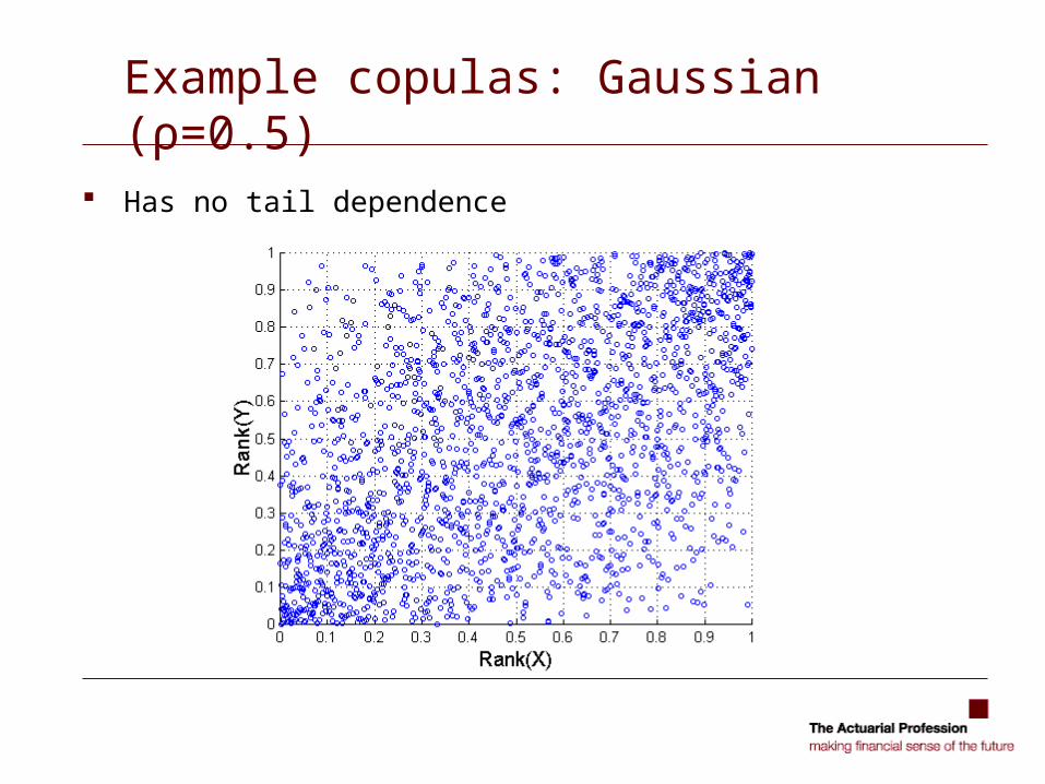
Example copulas: Gaussian (ρ=0.5)

Has no tail dependence

Example copulas: t

Does have tail dependence, same in both tails

Example copulas: Asymmetric t

Has tail dependence and skewness

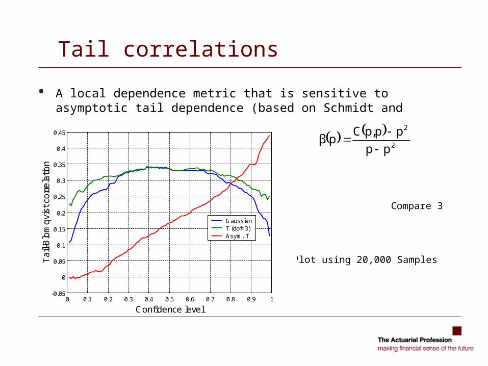
Tail correlations

A local dependence metric that is sensitive to asymptotic tail dependence (based on Schmidt and Schmid, 2006)

Left tail p=0

Right tail p=1

Compare 3 copulas

- Gaussian

- t

- Asymmetric t Plot using 20,000 Samples

Very unstable!

0 0.1 0.2 0.3 0.4 0.5 0.6 0.7 0.8 0.9 1-0.05

0

0.05

0.1

0.15

0.2

0.25

0.3

0.35

0.4

0.45

Confidence level

Ta

il-B

lom

qvi

st c

orr

ela

tion

Gaussian T (dof=3)Asym. T

2

2

pp

pp,pCpβ

Skew-rank correlations

Try to identify skewness from a small sample (of 20) Generalisation of rank correlation with a 3rd moment adjustment

The sensitivity to the 3rd joint moments of the

sample ranks increases with coefficient “a”.

a=0 gives the usual rank correlation.

0 2 4 6 8 10 12 14 16 18 20-0.1

-0.05

0

0.05

0.1

0.15

0.2

0.25

0.3

0.35

Coefficient a

Ske

w R

an

k C

orr

ela

tion

Gaussian T (dof=3)Asym. T

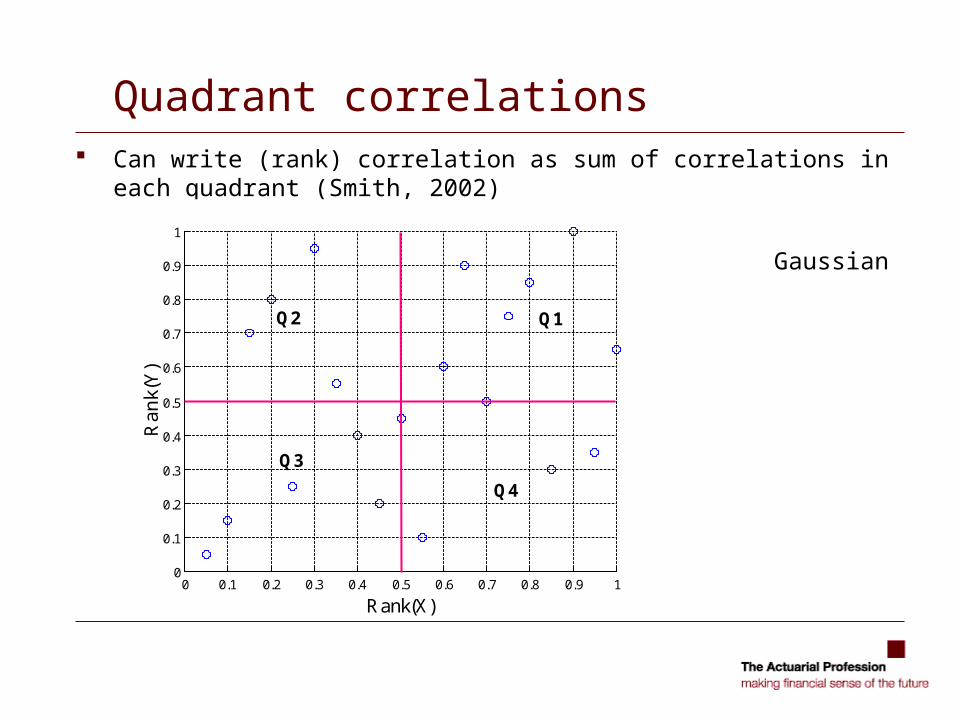
Quadrant correlations Can write (rank) correlation as sum of correlations in each quadrant

(Smith, 2002)

Gaussian copula

0 0.1 0.2 0.3 0.4 0.5 0.6 0.7 0.8 0.9 10

0.1

0.2

0.3

0.4

0.5

0.6

0.7

0.8

0.9

1

Rank(X)

Ra

nk(

Y)

Quadrant correlations Can write (rank) correlation as sum of correlations in each quadrant

(Smith, 2002)

Gaussian copula

0 0.1 0.2 0.3 0.4 0.5 0.6 0.7 0.8 0.9 10

0.1

0.2

0.3

0.4

0.5

0.6

0.7

0.8

0.9

1

Rank(X)

Ra

nk(

Y)

Q1

Q4

Q3

Q2

Quadrant correlations Can write (rank) correlation as sum of correlations in each quadrant

(Smith, 2002)

t copula

0 0.1 0.2 0.3 0.4 0.5 0.6 0.7 0.8 0.9 10

0.1

0.2

0.3

0.4

0.5

0.6

0.7

0.8

0.9

1

Rank(X)

Ra

nk(

Y)

Quadrant correlations Can write (rank) correlation as sum of correlations in each quadrant

(Smith, 2002)

Asymmetric t copula

0 0.1 0.2 0.3 0.4 0.5 0.6 0.7 0.8 0.9 10

0.1

0.2

0.3

0.4

0.5

0.6

0.7

0.8

0.9

1

Rank(X)

Ra

nk(

Y)

Quadrant correlations Plot the % breakdown of aggregate rank correlation to quadrants

0 1 2 3 4 5-4

-3

-2

-1

0

1

2

3

4

5

Quadrant

% B

rea

kdo

wn

of c

orr

ela

tion

to q

ua

dra

nts

Gaussian T (dof=3)Asym. T

Tip #2: Use judgement expertly

There are 3 ways of using expert judgement in model calibration Method 1

Ask underwriters and other experts for sources of correlation Make up some numbers

Method 2 Ask questions that experts can answer meaningfully Identify drivers of dependence Associate those with your copula models

Method 3 Adopt a full formal Bayesian framework Not quite there yet!

Tip #3: Understand your models

Copula models can often be expressed via factors (drivers) So not as ad-hoc as you may think Helps you chose an appropriate structure

Gaussian copula: n (or less!) additive factors determine correlation structure

t-copula: same as Gaussian with one additional multiplicative factor driving tail dependence, even for otherwise uncorrelated risks

Archimedean copulas (e.g. Gumbel, Clayton): there is one factor, conditional upon which all risks are independent

p-factor Archimedean copulas: as above, but can use more than one factor

Tip #4: Keep it simple

Modern DFA software offers you a wealth possibilities But you may be tempted to overparameterise your model A small number of parameters (drivers) will give you a better

chance of making meaningful (interpretable) choices You may even be able to do a bit of estimation

Tip #5: Use other models for reference

Suppose you have a peril model which you believe in But it doesn’t cover all your risks

Maybe the dependence structure that it implies between classes can be used as a proxy for risks that aren’t covered?

Fit a copula to the peril model simulations Loads of (pseudo-)data!

Alternatively suppose you have some particular pairs of risks for which you have more data This may help you get a feeling for sensible parameter ranges

Tip #6: Work backwards

See what diversification credits different copula choices imply Do they make sense? The argument is of course circular, but it may help involve people

in the thinking

Tip #7: Take care of your data

You may not have enough data today If you collect and maintain your data you’ll have more tomorrow

Tip #8: Adopt a positive attitude

It is no good complaining about fitting a copula ‘being impossible’ It is difficult but not impossible in principle Insisting on the difficulty does not make the problem of dependencies

go away

There are some things you can do Though they still may not work Shouldn’t you be used to this?

Literature I used for this talk

On most things: McNeil, Frey and Embrechts (2005), Quantitative Risk Management,

Princeton University Press.

On quadrant correlations and normal mixtures Smith (2002), ‘Dependent Tails’, 2002 GIRO Convention,

http://www.actuaries.org.uk/Display_Page.cgi?url=/giro2002/index.xml

A technical paper from which I pinched an idea or two: Schmidt and Schmid (2006) ‘Nonparametric Inference on Multivariate Versions

of Blomqvist's Beta and Related Measures of Tail Dependence’, http://www.uni-koeln.de/wiso-fak/wisostatsem/autoren/schmidt/publication.html

Sample literature on fitting copulas (yes it exists)

Genest and Rivest (1993), ‘Statistical inference procedures for bivariate Archimedean copulas,’ J. Amer. Statist. Assoc. 88, 1034-1043.

Joe (1997), Multivariate Models and Dependence Concepts, Chapman & Hall.

McNeil, Frey and Embrechts (2005), Quantitative Risk Management, Princeton University Press.

Denuit, Purcaru and Van Bellegem (2006), 'Bivariate archimedean copula modelling for censored data in nonlife insurance'. Journal of Actuarial Practice 13, 5-32.

Chen, Fan and Tsyrennikov (2006), ‘Efficient estimation of semiparametric multivariate copula models. J. Am. Stat. Assoc. 101, 1228-1240.

Appendix - dependence measures

Consider risks X and Y, with cdfs F and G. Let U=F(X), V=G(Y) Let X’=X-E[X], Y’=Y-E[Y], U’=U-E[U], V’=V-E[V] Assume sample of size n x={x1,…,xn } is the sample from random variable X etc

u={u1,…,un } are the normalised sample ranks of X, i.e. numbers 1/n, 2/n,…,1, but ordered in the same way as the elements of x.

Same for y, v.

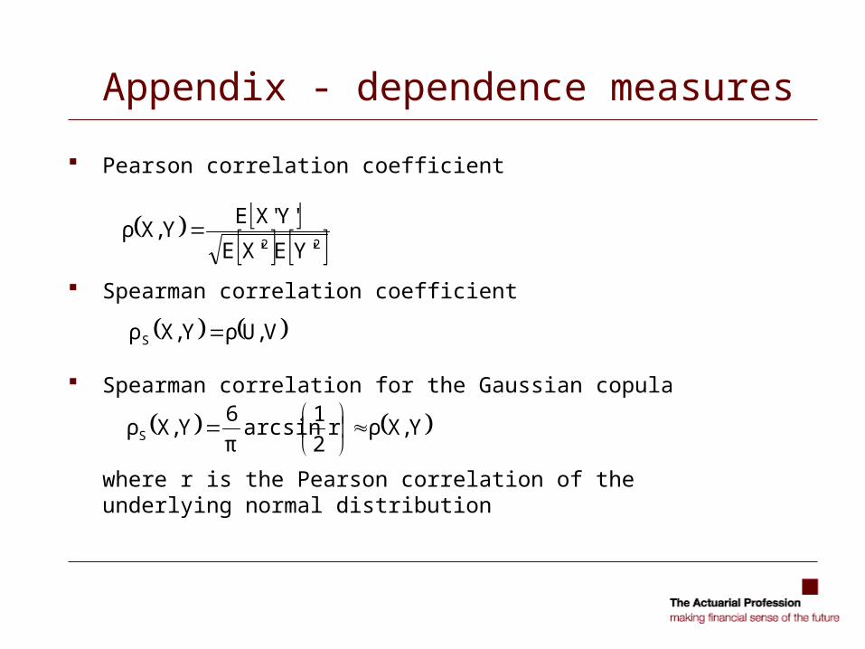
Appendix - dependence measures

Pearson correlation coefficient

Spearman correlation coefficient

Spearman correlation for the Gaussian copula

where r is the Pearson correlation of the underlying normal distribution

22 'YE'XE

'Y'XEY,Xρ

V,UρY,XρS

Y,Xρr2

1arcsin

π

6Y,XρS

Appendix - dependence measures

Kendall correlation coefficient (population version)

where is an independent copy of (X,Y) Kendall correlation coefficient (sample version)

Kendall correlation coefficient elliptical copulas (incl. Gaussian, t)

where r is the Pearson correlation of the underlying elliptical distribution

0Y~

YX~

XP0Y~

YX~

XPY,Xτ

)Y~

,X~

(

nji1ijij

1

yyxxsign2

nY,Xτ

rarcsinπ

2Y,Xτ

Appendix - dependence measures

Kendall correlation coefficient of the Pareto (flipped Clayton) copula

Copula function:

Kendall’s τ:

Kendall correlation coefficient of the Gumbel copula

Copula function:

Kendall’s τ:

θ/1θθ 1v1u11vuv,uC

θ/1θθ vlnulnexpv,uC

2θ

θ

θ

11

Appendix - dependence measures

“Tail-Blomqvist” correlation coefficient (Schmidt and Schmid, 2006)

where 0<p<1 and C is the copula of (X, Y) For we have asymptotic upper tail-dependence

For we have asymptotic lower tail-dependence

For sample version use the empirical copula:

2

2

pp

pp,pCp;Y,Xβ

0λp;Y,Xβlim U1p

0λp;Y,Xβlim L0p

2

2

pp

pp,pCp;Y,Xβ

n

n/jv,n/iu:)v,u(#

n

j,

n

iC kkkk

n

Appendix - dependence measures

“Skew-rank correlation”

Quadrant rank correlation (Smith, 2002)

etc, where I{A} is the indicator function of set A

3/233/133/133/232/122/12

22

S|'Y|E|'X|E|'Y|E|'X|Ea'YE'XE

'Y'XE'Y'XEa'Y'XEa;Y,Xρ

Y,XρY,XρY,XρY,XρY,Xρ SSSSS

22S

'VE'UE

,0'V,0'U'V'UEY,Xρ

I

22S'VE'UE

,0'V,0'U'V'UEY,Xρ

I