flat panel detector-based cone beam ct: …
TRANSCRIPT
FLAT PANEL DETECTOR-BASED CONE BEAM CT:
RECONSTRUCTION IMPLEMENTATION AND APPLICATIONS
FOR DYNAMIC IMAGING
by
Dong Yang
Submitted in Partial Fulfillment
of the
Requirements for the Degree
Doctor of Philosophy
Supervised by
Professor Ruola Ning
Department of Electrical and Computer Engineering
The College
School of Engineering and Applied Sciences
University of Rochester
Rochester, New York
12/10/2007
ii
Curriculum Vitae
The author was born in Chongqing, P.R. China on Oct. 23rd, 1968. He attended The
Chinese Air Force Radar College from 1986 to 1990, and graduated with a Bachelor
of Radar Engineering degree in 1990. He attended Chongqing University from 1995
to 1998, and graduated with a Master of Biomedical Engineering degree in 1998. He
came to America in 2000 and studied in the Center of Imaging Science in Rochester
Institute of Technology as a PhD candidate. He transferred to the University of
Rochester in the spring of 2003 and continued his graduate studies in the Department
of Electrical and Computer Engineering and Department of Imaging Sciences. He
received the research assistantship since then. He pursued his research in Image
Reconstruction in X-ray cone beam CT under the direction of Professor Ruola Ning
and received the Master of Arts degree from the University of Rochester in 2004.

iii
Acknowledgements
I am grateful for the support and help from my advisor, Dr. Ruola Ning. His
consistent academic guidance, financial support, and encouragement make me
accomplish this dissertation. Five years studying under his direction is an enjoyable
and invaluable experience that will benefit me throughout my life and career.
Furthermore, special thanks go to him for letting me witness the development of the
Cone Beam Breast CT and be involved in the further improvement.
I also want to thank David Conover, manager of Cone Beam CT Lab (in the
Department of Imaging Sciences at University of Rochester) who is always available
whenever I want to do experiment to test the conceptual ideas. His suggestions and
insights helped me a lot.
It is my fortune to have Professor Mark F. Bocko, Dr. Wendi Heinzelman, Dr.
Andrew J. Berger and Dr. Jianhui Zhong on my thesis committee. I am very grateful
for their instructive comments and suggestions.
During my five years at the University of Rochester, I have received a lot of help
from people in our lab. Many thanks to my past and current co-workers: Yong Yu,
Shaohua Liu, Xianghua Lu; my fellow graduate students Bentacourt Ricardo, Yang
Zhang, Weixing Cai, Xiaohua Zhang. A special thank also goes to Michael
Barravecchia for his assistance in setting up the mouse dynamic study.
I also want to acknowledge funding supports from the NIH Grants 8 R01 EB 002775,
R01 9 HL078181, 4 R33 CA94300.
Finally, I sincerely thank my wife, my son, my parents, and my mother-in-law for
being very understanding and supportive.
iv
Abstract
X-ray Computed Tomography has experienced several generations of development
from single detector cell, several detector cells, an array of detector cells, through
multiple rows of detector cells and two-dimensional detector cells. The introduction
of the area detector is one of the key characteristics of the cone beam CT which
represents a breakthrough in terms of the real three-dimensional isotropic resolution,
large Z-coverage. Dedicated object scanning such as breast cone beam CT and
dentomaxillofacial cone beam CT are made possible.
The area detector which is large enough to cover the entire organs, such as the heart,
the kidneys, the brain, or a substantial part of a lung, in one axial scan could bring a
new quality to medical CT. With these new systems, real dynamic volume scanning
would become possible, and a whole spectrum of new applications, such as functional
or volume perfusion studies, could arise. Challenges also come with the excitement of
cone beam CT, such as beam hardening, scattering, non-uniform distribution over the
area detector, and gain non-linearity at each detector cell, and cone angle induced
reconstruction artifacts if only a circular scan is employed.
In this thesis, a heuristically weighted function was developed for the cone beam half
scan circular scanning scheme so as to improve the temporal resolution and suppress
the motion artifacts; a composite hybrid scanning scheme was proposed to correct the
cone angle-induced artifacts for the cone beam breast imaging CT prototype. A
dynamic experimental phantom and an animal (mouse) study was conducted to
develop a dynamic scanning protocol to testify the feasibility of the angiogenesis (i.e.
to differentiate the benign and malignant tumor by depicting the dynamic uptake of
the contrast agent in vasculature) imaging associated with the cone beam breast
imaging CT.
v
Table of Contents
Chapter 1 Background of Cone Beam CT (CBCT).................................................. 1
1.1 The history of CT..................................................................................... 1
1.1.1 The generations of CT technology........................................................... 2
1.1.2 The spiral CT ........................................................................................... 7
1.1.2.1 The single-row spiral CT .......................................................... 8
1.1.2.2 The multi-row spiral CT ........................................................... 9
1.2 Motivations of the CBCT....................................................................... 10
1.3 Current applications and challenges with CBCT................................... 11
1.4 Outline of the thesis ............................................................................... 14
Chapter 2 Circular CBCT image reconstruction by filtered backprojection .......... 16
2.1 The Radon Transform (RT) and Fourier Central Slice (FCS) Theorem 16
2.1.1 Two-dimensional RT and FCS theorem ................................................ 16
2.1.2 Three-dimensional RT and FCS theorem .............................................. 19
2.2 Two-dimensional FBP image reconstruction......................................... 21
2.2.1 2-D parallel beam image reconstruction ................................................ 21
2.2.2 Two-dimensional fan beam image reconstruction................................. 24
2.2.3 Two-dimensional fan beam half scan image reconstruction.................. 25
2.3 Three-dimensional FBP image reconstruction....................................... 28
2.3.1 The data sufficient condition with cone beam reconstruction ............... 28
2.3.2 The approximate reconstruction ............................................................ 31
2.3.3 The exact reconstruction ........................................................................ 33
Chapter 3 Circle plus partial helical line segment scan with Cone Beam Breast CT (CBBCT) ................................................................................................................ 36
3.1 The development of cone beam breast CT ............................................ 36
3.2 The circle plus partial helical line scanning (CHL) ............................... 38
3.2.1 Data acquisition analysis in terms of Radon domain............................. 38
3.2.2 Scanning design for CHL and straight line (CL) trajectory................... 43
3.3 FBP reconstruction algorithm associated with different scanning schemes ................................................................................................................ 45
vi
3.3.1 Algorithm for CHL scheme ................................................................... 45
3.3.2 Derivation of the redundant window function ),( ϕlwiZ with helical line
scan ................................................................................................................ 48
3.3.3 Algorithm for CL scheme ...................................................................... 50
3.4 Performance evaluation through computer simulation .......................... 52
3.4.1 Description of the numerical breast phantom & scanning parameters .. 52
3.4.2 Performance with and without the truncation window.......................... 54
3.4.3 Performance with π- and 2π-scanning range in partial helical line scans.. ................................................................................................................ 54
3.4.4 Performance with different sampling intervals in partial helical line scans ................................................................................................................ 55
3.4.5 Performance with different sampling intervals in straight line scan...... 55
3.4.6 Profile comparison between phantom, MFDK, CHL and CL scanning schemes ............................................................................................................... 55
3.5 The Experimental Breast Phantom Study .............................................. 56
3.6 Discussion and conclusion..................................................................... 57
Chapter 4 Circular Half-Scan Cone Beam Reconstruction .................................... 69
4.1 Traditional circular cone beam half-scan scheme.................................. 69
4.1.1 Traditional circular FDK cone beam half-scan algorithm ..................... 70
4.2 Modified circular FDK cone beam half-scan algorithm........................ 73
4.2.1 Heuristic circular cone beam half-scan weighting scheme.................... 74
4.2.2 Supplementary FBP term in circular cone beam half-scan reconstruction ................................................................................................................ 76
4.3 Performance evaluation through computer simulation .......................... 79
4.3.1 The weighting coefficients distribution comparison of FDK-HSCW and FDK-HSFW ........................................................................................................ 80
4.3.2 Comparison of FDK-FS, MFDK-HS and FDK-HSFW on Shepp-Logan phantom with noise-free projection data............................................................. 80
4.3.3 Comparison of FDK-FS and MFDK-HS on Shepp-Logan phantom with simulated Poisson noise in projection data ......................................................... 81
4.3.4 Comparison of FDK-FS, MFDK-HS on disc phantom ......................... 81
4.4 Performance evaluation through practical experiment .......................... 82
4.4.1 Phantom study........................................................................................ 82
vii
4.4.2 Mouse study ........................................................................................... 83
4.5 Discussion and conclusion..................................................................... 84
Chapter 5 CBBCT Dynamic Study ........................................................................ 95
5.1 Background and purpose of the dynamic study..................................... 95
5.2 CBBCT dynamic study based on computer simulation......................... 96
5.2.1 The scanning parameters associated with the computer simulation ...... 96
5.2.2 The scanning design............................................................................... 98
5.2.3 The results.............................................................................................. 99
5.2.3.1 A-T curve comparison based on gantry speed of 1 second per circle ................................................................................................. 99
5.2.3.2 A-T curve comparison based on gantry speed of 5 seconds per circle ............................................................................................... 100
5.2.3.3 A-T curve comparison based on gantry speed of 10 seconds per circle ............................................................................................... 101
5.2.3.4 A-T curve comparison between HS and FS based on different scanning speed ..................................................................................... 102
5.2.3.5 A-T curve comparison between different time interval under the same scanning scheme ................................................................... 103
5.3 Experimental phantom and mice study................................................ 104
5.3.1 Phantom study...................................................................................... 104
5.3.1.1 Phantom scanning protocol................................................... 105
5.3.1.2 Data analysis ......................................................................... 106
5.3.2 Mice study............................................................................................ 107
5.3.2.1 Mice dynamic scanning protocol .......................................... 107
5.3.2.2 Data analysis ......................................................................... 108
5.4 Discussion and conclusion................................................................... 109
Chapter 6 Summary and future work ................................................................... 116
6.1 Summary .............................................................................................. 116
6.2 Future work.......................................................................................... 119
6.2.1 Patient dynamic study .......................................................................... 119
6.2.2 De-noising and improvement of spatial resolution.............................. 119
Papers and patent related to this thesis ..................................................................... 121

viii
Bibliography ............................................................................................................. 123
ix
List of Tables Table 3-1 Partial helical line scanning parameters .................................................. 53
Table 3-2 Straight line scanning parameters............................................................ 54
Table 4-1 Numerical parameters for low contrast Shepp-Logan phantom.............. 79
Table 4-2 Scan and reconstruction parameters for the breast imaging phantom (BIP)
and mouse (M) .................................................................................................... 82
Table 4-3 Reconstruction results for Breast Imaging Phantom............................... 83
Table 5-1 Numerical parameters for low contrast Shepp-Logan phantom.............. 98
x
List of Figures
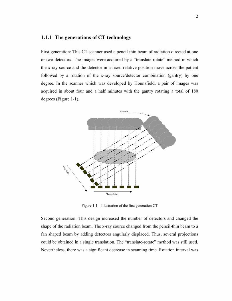
Figure 1-1 Illustration of the first generation CT....................................................... 2
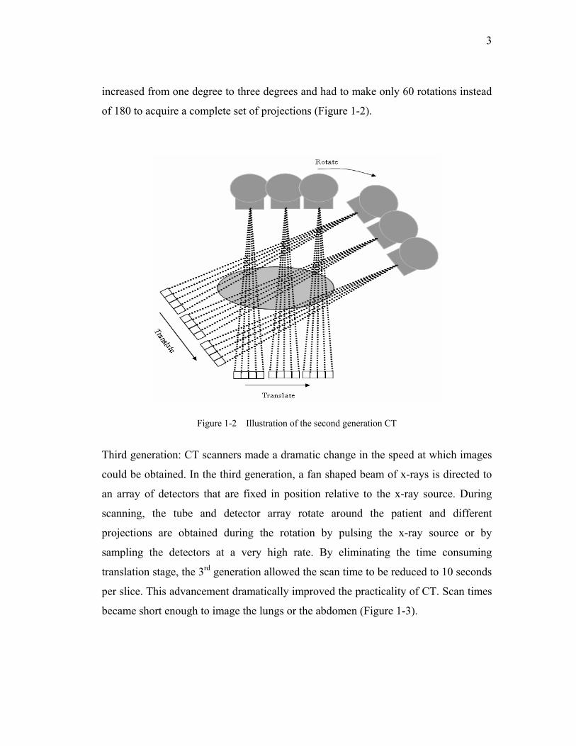
Figure 1-2 Illustration of the second generation CT.................................................. 3
Figure 1-3 Illustration of the third generation CT ..................................................... 4
Figure 1-4 Illustration of the fourth generation CT ................................................... 5
Figure 1-5 Illustration of the fifth generation CT (EBCT); (a) Sagittal view of the
EBCT; (b) Cross sectional view of the EBCT...................................................... 6
Figure 1-6 Illustration of conventional CT using step shoot mode to get the volume
information............................................................................................................ 7
Figure 1-7 Illustration of single slice spiral CT......................................................... 8
Figure 1-8 Illustration of multi-slice spiral CT........................................................ 10
Figure 1-9 Illustration of working snapshot of the OBI (adopted from Varian
product website).................................................................................................. 12
Figure 2-1 Illustration of line integral defined in the object coordinate system...... 17
Figure 2-2 Illustrations of three-dimensional Radon transform defined in the object
coordinate system................................................................................................ 19
Figure 2-3 Illustration of the 3D Fourier Central Slice Theorem ............................ 20
Figure 2-4 Illustration of two-dimensional parallel beam projection ...................... 22
Figure 2-5 Geometric illustration of 2D fan beam projection ................................. 24
xi
Figure 2-6 Illustrations of sinogram for parallel and for fan beam projections with π
and π + 2λ angular range; (a) parallel beam with π range; (b) fan beam with π
range; (c) parallel beam with π + 2λ range;........................................................ 26
Figure 2-7 Illustration of the relationship between 3D Radon data and X-ray cone
beam projection data ........................................................................................... 30
Figure 2-8 Geometric illustration of a circular scan. ............................................... 31
Figure 2-9 Sectional view of the three-dimensional radon data of the object with the
radius R2 acquired in a circular scan ................................................................... 33
Figure 3-1 Illustration of the three-dimensional Radon transform and the Radon
shell in the object space-based on cone beam geometry..................................... 39
Figure 3-2 Illustration of the radon point in the radon domain within the object
Radon support ..................................................................................................... 40
Figure 3-3 Illustration of the circle plus partial helical line scan ............................ 43
Figure 3-4 Illustration of the straight line scan to achieve an exact reconstruction 45
Figure 3-5 The geometric illustration of the same Radon value defined in the object
coordinate system and the reconstruction coordinate system associated with
partial helical line scan........................................................................................ 47
Figure 3-6 Illustration of straight line scanning....................................................... 51
Figure 3-7 The comparison of the corresponding effects on reconstruction based on
processed radon data with and without a truncation window; (a) The processed
line projection data, mathematically represented by ),( ϕlHiZ in formula (3.5);
(b) The corresponding central sagittal reconstruction image of a circle plus line
scheme where the display window is [-300 -100]; (c) The central sagittal
phantom image; (d) The processed line projection data, mathematically
xii
represented by ),( ϕlHiZ in formula (3.5) but without a truncation window
),( ϕlwiZtr ; (e) The corresponding central sagittal reconstruction image of a circle
plus line scheme where the display window is [-300 -100]................................ 61
Figure 3-8 The central sagittal images based on helical line scanning range of π, 2π
respectively; (a) π range within a line scan; (b) 2π range within a line scan...... 61
Figure 3-9 Central sagittal image comparison between MFDK, phantom and partial
helical line term with different sampling interval; (a) FDK; (b) Hui term; (c)
MFDK; (d) MFDK; (e) HL recon (32 points); (f) MFDK + HL (32 points); (g)
MFDK; (h) HL recon (64 points); (i) MFDK + HL (64 points); (j) Phantom.... 62
Figure 3-10 The central sagittal image comparison between phantom and CL
scanning scheme with different sampling interval along straight line trajectory;
(a) FDK; (b) Line scan (556 points); (c) FDK + Line scan (556 points); (d) Line
scan (210 points); (e) FDK + Line scan (210 points); (f) Line scan (64 points); (g)
FDK + Line scan (64 points); (h) Phantom ........................................................ 63
Figure 3-11 Profile comparison between phantom, MFDK, and MFDK plus
different auxiliary scanning schemes; (a) Phantom image with three profile lines;
(b) Profile comparison along the middle vertical line in (a); (c) Profile
comparison along the left vertical line in (a); (d) Profile comparison along the
horizontal line in (a)............................................................................................ 65
Figure 3-12 Axial image at z = 84.63 mm for (a) and (b) and the coronal image
where y = -7.4 mm for (c) and (d). They are displayed with the same window [-
640 –520]. The line profile comparison along white vertical and horizontal lines
in (c) and (d) are shown in (e) and (f) respectively. The first projection image
during the HL scan where the projection angle is 0 and z = 30 mm is shown in (g)
with a very narrow display window so one can appreciate the correctness of the
xiii
geometrical deformation around the nipple area of the circle plus partial helical
line in (d)............................................................................................................. 68
Figure 4-1 Equal space cone beam geometry with the circular scans ..................... 71
Figure 4-2 Illustration of redundant regions in terms of projection angle in circular
fan-beam half-scan.............................................................................................. 74
Figure 4-3 Geometric illustration of relationship between cone beam projection data
and Radon data.................................................................................................... 77
Figure 4-4 Weighting coefficients comparison between FDK-HSFW and FDK-
HSCW when β = 460 and when β = 1920; (a) FDK-HSFW (β = 460); (b) FDK-
HSCW (β = 460); (c) FDK-HSFW (β = 1920); (d) FDK-HSCW (β = 1920) ...... 86
Figure 4-5 Reconstructed sagittal images from different FDK schemes at X = 0 mm;
(a) FDK-FS; (b) FDK-HSFW; (c) MFDK-HS; (d) Phantom.............................. 87
Figure 4-6 Profile comparison of reconstructed sagittal images from different FDK
schemes at X = 0 mm; (a) Vertical line profile as shown in Figure 4-5(d); (b)
Horizontal line profile as shown in Figure 4-5(d) .............................................. 88
Figure 4-7 Reconstructed sagittal images from different FDK schemes at X = 0 mm
with different simulated noise level; (a) FDK-FS (1800 mR); (b) FDK-HSFW
(1048 mR); (c) MFDK-HS (1800 mR); ............................................................... 89
Figure 4-8 Profile comparison as in Figure 4-6(a) but with simulated noise level; the
exposure level for FDK-FS is 1800 mR while for MFDKHS is 1048 mR;......... 90
Figure 4-9 Reconstructed central sagittal image and profile comparison from
different FDK schemes; (a) FDK-FS; (b) MFDK-HS; (c) Phantom; (d) Profile
along y=the with line shown in (c) ..................................................................... 91
xiv
Figure 4-10 Cross sectional images of the breast imaging phantom with different
size of simulated tumors reconstructed from different FDK schemes under
different exposure level; (a) FDK-FS (725 mR); (b) MFDK-HS (390 mR); (c)
MFDK-HS (725 mR)........................................................................................... 92
Figure 4-11 Three dimensional rendering mouse images reconstructed by half and
full scanning schemes; (a) MFDK-HS; (b) FDK-FS .......................................... 93
Figure 4-12 Gray scale sagittal mouse images reconstructed by half and full
scanning schemes; (a) MFDK-HS; (b) FDK-FS................................................. 94
Figure 5-1 Simulated tumor attenuation coefficient time (A-T) curve in the length
of 20 seconds....................................................................................................... 97
Figure 5-2 Illustration of the reconstructed images in time series based on
continuous scan................................................................................................... 99
Figure 5-3 A-T curve comparison based on gantry rotation speed of 1 second per
circle.................................................................................................................. 100
Figure 5-4 A-T curve comparison based on gantry rotation speed of 5 seconds per
circle.................................................................................................................. 101
Figure 5-5 A-T curve comparison based on gantry rotation speed of 10 seconds per
circle.................................................................................................................. 102
Figure 5-6 A-T curves comparison between HS and FS under different gantry
rotation speed .................................................................................................... 103
Figure 5-7 A-T curve comparison with HS under different interval value based on
the same gantry rotation speed.......................................................................... 104
Figure 5-8 Experimental setup for the dynamic phantom study............................ 105
xv
Figure 5-9 A-T curve comparison between projection data, half scan and full scan
data.................................................................................................................... 106
Figure 5-10 Experiment setup for the mouse dynamic study ................................ 108
Figure 5-11 Sagittal images of the reconstructed mouse from different FDK
schemes; (a) FDK-FS ( # of projections = 300); (b) MFDK-HS ( # of projections
= 160) ................................................................................................................ 111
Figure 5-12 Illustration of the 3D rendering mouse image; (a) 3D rendering of
whole mouse image during dynamic phase; (b) zoomed part to show the
segmented blood vessels for evaluation............................................................ 113
Figure 5-13 Illustration motion-induced artifacts suppression by MFDK-HS; (a)
FDK-FS; (b) MFDK-HS................................................................................... 114
Figure 5-14 A-T curve comparison between half scan and full scan data in mouse
dynamic study ................................................................................................... 115
Figure 6-1 Demonstration of suppression of motion artifacts by choosing proper
starting point for reconstruction in half scanning scheme, display window is [-
250 300]; (a) Full scan reconstruction; (b) Half scan reconstruction where
starting projection index for reconstruction is 130 ........................................... 118
1
Chapter 1 Background of Cone Beam CT (CBCT)
1.1 The history of CT
The onset of X-ray CT was based on two facts; one is the discovery of X-rays by
RÖntgen in 1895, and the other is the mathematical foundation presented by Radon in
1917. The fundamental concept underlying the technique of computed tomography is
the capability of reconstructing or synthesizing a cross-section of the internal
structure of an object from multiple projections of a collimated x-ray beam passing
through the object. The mathematical basis for reconstruction of an object from
multiple projections through the object dates back to the work of the Austrian
mathematician J. Radon working in gravitational theory in 1917 [1]. Radon
demonstrated mathematically that a two- or three- dimensional object could be
reproduced from the infinite set of all its projections. The physical application of the
concept of reconstruction from multiple transmitted projections by Cormack and
Hounsfield [2] enabled them to share the Nobel Prize in Physiology and Medicine in
1979 for their contributions to the development of computed tomography. Since then,
this modality has evolved into an essential diagnostic imaging tool for a continually
increasing variety of clinical applications.
2
1.1.1 The generations of CT technology
First generation: This CT scanner used a pencil-thin beam of radiation directed at one
or two detectors. The images were acquired by a “translate-rotate” method in which
the x-ray source and the detector in a fixed relative position move across the patient
followed by a rotation of the x-ray source/detector combination (gantry) by one
degree. In the scanner which was developed by Hounsfield, a pair of images was
acquired in about four and a half minutes with the gantry rotating a total of 180
degrees (Figure 1-1).
Figure 1-1 Illustration of the first generation CT
Second generation: This design increased the number of detectors and changed the
shape of the radiation beam. The x-ray source changed from the pencil-thin beam to a
fan shaped beam by adding detectors angularly displaced. Thus, several projections
could be obtained in a single translation. The “translate-rotate” method was still used.
Nevertheless, there was a significant decrease in scanning time. Rotation interval was
3
increased from one degree to three degrees and had to make only 60 rotations instead
of 180 to acquire a complete set of projections (Figure 1-2).
Figure 1-2 Illustration of the second generation CT
Third generation: CT scanners made a dramatic change in the speed at which images
could be obtained. In the third generation, a fan shaped beam of x-rays is directed to
an array of detectors that are fixed in position relative to the x-ray source. During
scanning, the tube and detector array rotate around the patient and different
projections are obtained during the rotation by pulsing the x-ray source or by
sampling the detectors at a very high rate. By eliminating the time consuming
translation stage, the 3rd generation allowed the scan time to be reduced to 10 seconds
per slice. This advancement dramatically improved the practicality of CT. Scan times
became short enough to image the lungs or the abdomen (Figure 1-3).
4
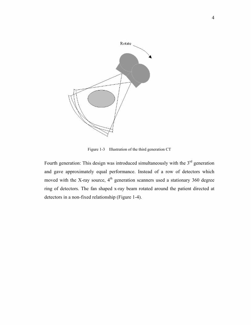
Figure 1-3 Illustration of the third generation CT
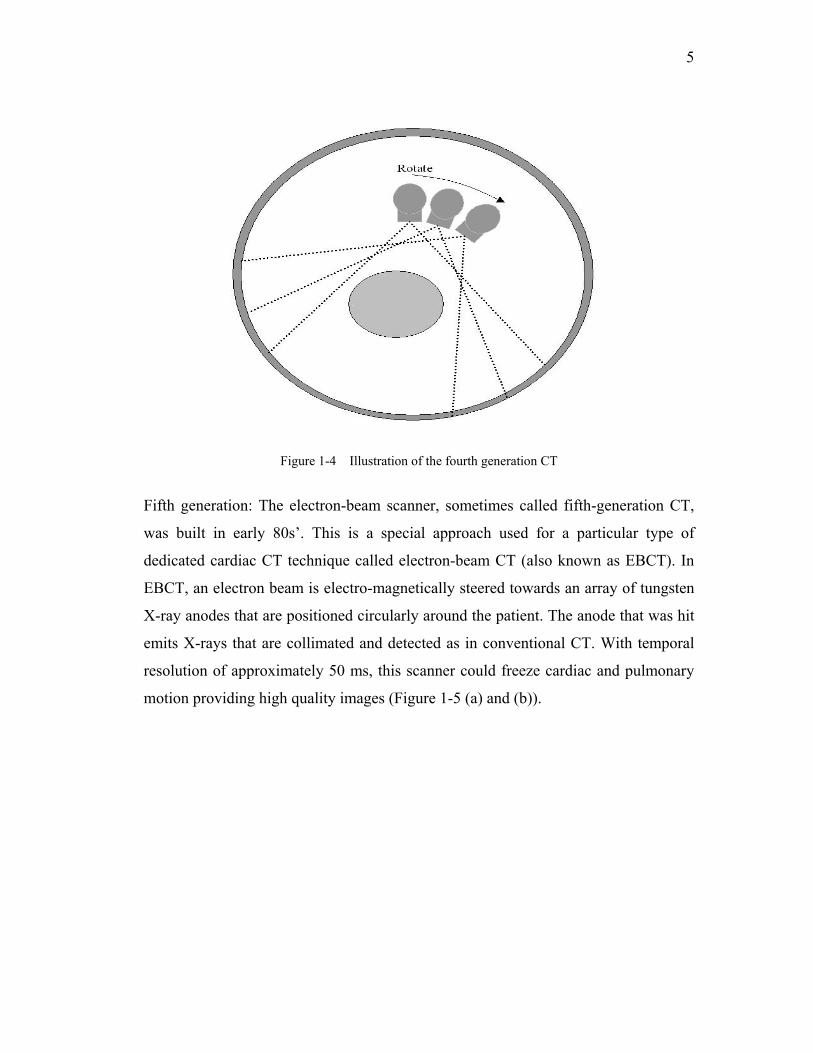
Fourth generation: This design was introduced simultaneously with the 3rd generation
and gave approximately equal performance. Instead of a row of detectors which
moved with the X-ray source, 4th generation scanners used a stationary 360 degree
ring of detectors. The fan shaped x-ray beam rotated around the patient directed at
detectors in a non-fixed relationship (Figure 1-4).
5
Figure 1-4 Illustration of the fourth generation CT
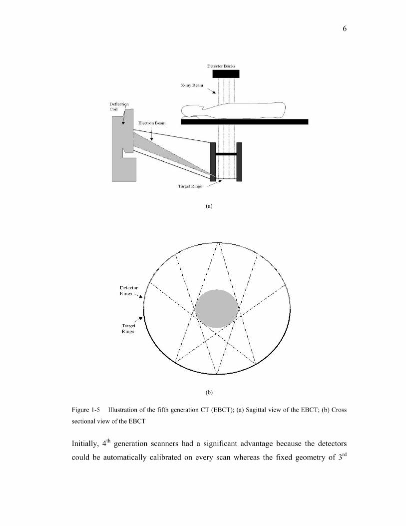
Fifth generation: The electron-beam scanner, sometimes called fifth-generation CT,
was built in early 80s’. This is a special approach used for a particular type of
dedicated cardiac CT technique called electron-beam CT (also known as EBCT). In
EBCT, an electron beam is electro-magnetically steered towards an array of tungsten
X-ray anodes that are positioned circularly around the patient. The anode that was hit
emits X-rays that are collimated and detected as in conventional CT. With temporal
resolution of approximately 50 ms, this scanner could freeze cardiac and pulmonary
motion providing high quality images (Figure 1-5 (a) and (b)).
6
(a)
(b)
Figure 1-5 Illustration of the fifth generation CT (EBCT); (a) Sagittal view of the EBCT; (b) Cross
sectional view of the EBCT
Initially, 4th generation scanners had a significant advantage because the detectors
could be automatically calibrated on every scan whereas the fixed geometry of 3rd
7
generation scanners was especially sensitive to detector mis-calibration (causing ring
artifacts). Additionally, because the detectors were subject to movement and vibration,
their calibration could drift significantly. However all modern medical scanners are of
3rd generation design because modern solid-state detectors are sufficiently stable that
calibration for each image is no longer required. The 4th generation scanners'
inefficient use of detectors made them considerably more expensive than 3rd
generation scanners. Furthermore, they were more sensitive to artifacts because the
non-fixed relationship to the x-ray source made it impossible to reject scattered
radiation.
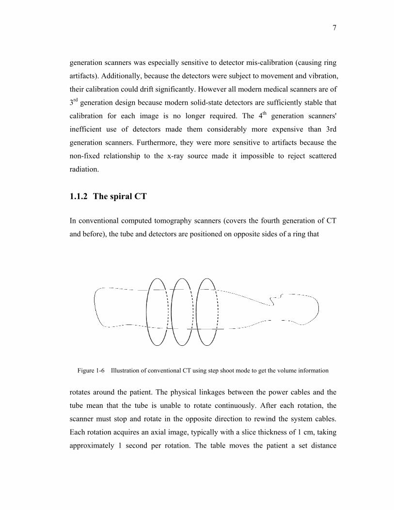
1.1.2 The spiral CT
In conventional computed tomography scanners (covers the fourth generation of CT
and before), the tube and detectors are positioned on opposite sides of a ring that
Figure 1-6 Illustration of conventional CT using step shoot mode to get the volume information
rotates around the patient. The physical linkages between the power cables and the
tube mean that the tube is unable to rotate continuously. After each rotation, the
scanner must stop and rotate in the opposite direction to rewind the system cables.
Each rotation acquires an axial image, typically with a slice thickness of 1 cm, taking
approximately 1 second per rotation. The table moves the patient a set distance
8
through the scanner each slice (Figure 1-6). Conventional CT has some limitations.
The scan time is slow, and the scans are prone to artifacts caused by movement or
breathing. The scanners have a poor ability to reformat in different planes; studies of
dynamic contrast are impossible; and small lesions between slices may be missed.
The technological developments in two areas [3], slip-ring power gantry and high
power x-ray tube, has created a renaissance of the spiral CT, which is used to combat
all the limitations of conventional CT aforementioned.
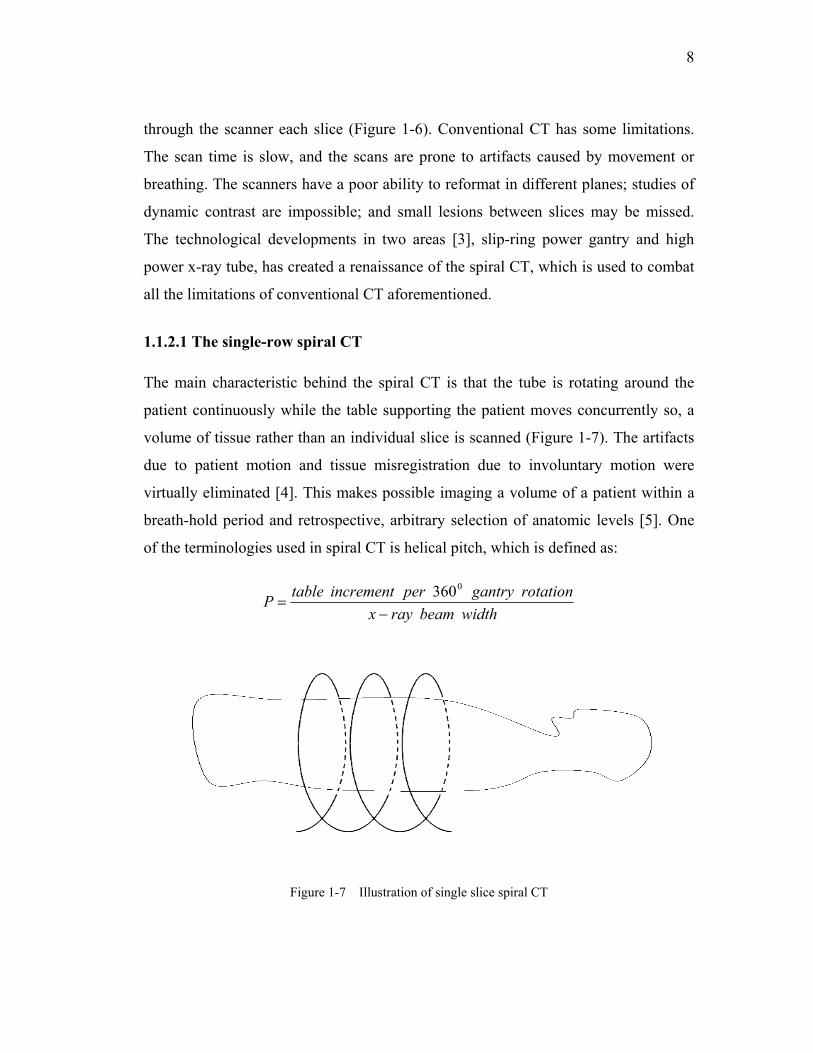
1.1.2.1 The single-row spiral CT
The main characteristic behind the spiral CT is that the tube is rotating around the
patient continuously while the table supporting the patient moves concurrently so, a
volume of tissue rather than an individual slice is scanned (Figure 1-7). The artifacts
due to patient motion and tissue misregistration due to involuntary motion were
virtually eliminated [4]. This makes possible imaging a volume of a patient within a
breath-hold period and retrospective, arbitrary selection of anatomic levels [5]. One
of the terminologies used in spiral CT is helical pitch, which is defined as:
widthbeamrayxrotationgantryperincrementtableP
−=
0360
Figure 1-7 Illustration of single slice spiral CT
9
Approximate isotropic (i.e., each image voxel is of equal dimension in all three
spatial axes) resolution could be obtained with the thinnest (~ 1-mm) section width at
a pitch of 1, but this could only be done over relatively short lengths due to the X-ray
tube and breath-hold limitations (usually 25-30 seconds). If a large scanning range,
such as the entire thorax or abdomen (30-cm), has to be covered within a single
breathhold, a thick collimation of 5 to 8-mm must be used. Although the in-plane
resolution of a CT image depends on the system geometry and on the reconstruction
kernel selected by the user, the longitudinal (z-) resolution is determined by the
collimated slice width and the spiral interpolation algorithm. Using a thick
collimation of 5 to 8-mm will result in a considerable mismatch between the
longitudinal and the in-plane resolution [6].
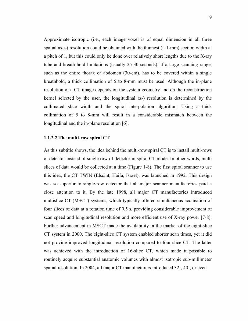
1.1.2.2 The multi-row spiral CT
As this subtitle shows, the idea behind the multi-row spiral CT is to install multi-rows
of detector instead of single row of detector in spiral CT mode. In other words, multi
slices of data would be collected at a time (Figure 1-8). The first spiral scanner to use
this idea, the CT TWIN (Elscint, Haifa, Israel), was launched in 1992. This design
was so superior to single-row detector that all major scanner manufactories paid a
close attention to it. By the late 1998, all major CT manufactories introduced
multislice CT (MSCT) systems, which typically offered simultaneous acquisition of
four slices of data at a rotation time of 0.5 s, providing considerable improvement of
scan speed and longitudinal resolution and more efficient use of X-ray power [7-8].
Further advancement in MSCT made the availability in the market of the eight-slice
CT system in 2000. The eight-slice CT system enabled shorter scan times, yet it did
not provide improved longitudinal resolution compared to four-slice CT. The latter
was achieved with the introduction of 16-slice CT, which made it possible to
routinely acquire substantial anatomic volumes with almost isotropic sub-millimeter
spatial resolution. In 2004, all major CT manufacturers introduced 32-, 40-, or even

10
Figure 1-8 Illustration of multi-slice spiral CT
64-slice CT simultaneously. Some of these scanners use refined z-sampling
techniques enabled by a periodic motion of the focal spot in the z-direction (z-flying
focal spot) to further enhance longitudinal resolution and image quality in clinical
routine [9]. With the most recent MSCT systems, CT angiographic examination with
sub-millimeter resolution in the pure arterial phase will become feasible even for
extended anatomic ranges. The logical development of MSCT is to increase the
number of detector arrays. The resulting clinical benefits, however, may not be
substantial and have to be carefully considered in the light of the necessary technical
efforts.
1.2 Motivations of the CBCT
For general anatomic imaging, MSCT is sufficient to provide enough information and
evolve into the most widely used diagnostic modality for routine examinations,
especially in emergency situations or for oncology staging. Even though the most
current MSCT can provide unprecedented improvement in terms of longitudinal
resolution and temporal resolution, the largest coverage in the longitudinal direction
is 40 mm; Due to the upper limit of the gravitational force, the tube and detector
assembles can bear, the gantry rotation speed can not be increased unlimitedly. These
11
disadvantages pose a limit of application of MSCT on real volume functional and
perfusion studies. For example, in cardiac imaging, the most current 64-slice CT
perform imaging of coronary artery and ventricular motion, and myocardial perfusion
with a longitudinal resolution of 0.5-mm and a temporal resolution of ~ 120-150
milliseconds using a multi-segmental algorithm, but the acquisition typically takes
~10 seconds. During this acquisition period, if the heart rhythm is not regular,
banding artifacts appear in the final reconstructed images. In contrast, one rotation of
256-slice CBCT with 1 s rotation speed can acquire the data of the entire heart and
coronary arteries with 0.5-mm isotropic voxel resolution without banding artifacts
[10-11]. The introduction of area detectors, one of the key characteristics of CBCT,
that is large enough to cover the entire organs, such as the heart, the kidneys, the
brain, or a substantial part of a lung, in one axial scan (~ 120 mm or more scan range)
could bring a new tool to medical CT. With these new systems, real dynamic volume
scanning would become possible; A whole spectrum of new applications, such as
functional or volume perfusion studies, could arise. For some special applications
where MSCT is not suitable, CBCT will play its dedicated role [12]. The combination
of area detectors with fast gantry speed is a promising technical concept for medical
CT systems.
1.3 Current applications and challenges with CBCT
Cone beam CT has been studied in the past two decades. The early studies were
mainly focused on the algorithms development, which we will touch in the next
chapter. The majority of this work was initially motivated by radiotherapy treatment
planning applications [13-17]. The medical diagnostic benefits of CBCT were studied
starting from middle 80’s [18-25]. The imaging performance was limited by the low
detection quantum efficiency of the combined image intensifier (II) and CCD
detectors used in these studies. The transition form CCD-and-II to flat panel detector
12
(FPD) marked a realistic applicability of the CBCT to clinical applications [26-33].
This is because the FPD does not have the interference resulting from pin cushion, S
distortion and veiling glare that exist in the CCD-and-II detector, and is more
spatially compact than a CCD-and-II detector. The most recent medical application
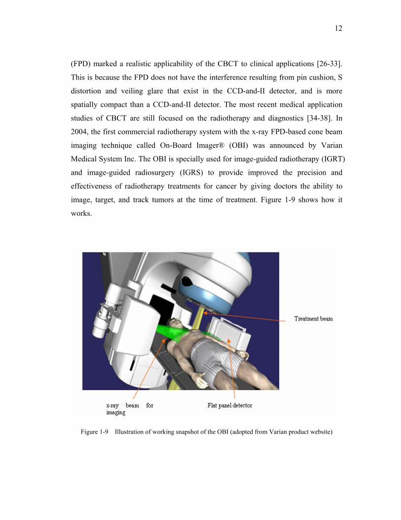
studies of CBCT are still focused on the radiotherapy and diagnostics [34-38]. In
2004, the first commercial radiotherapy system with the x-ray FPD-based cone beam
imaging technique called On-Board Imager® (OBI) was announced by Varian
Medical System Inc. The OBI is specially used for image-guided radiotherapy (IGRT)
and image-guided radiosurgery (IGRS) to provide improved the precision and
effectiveness of radiotherapy treatments for cancer by giving doctors the ability to
image, target, and track tumors at the time of treatment. Figure 1-9 shows how it
works.
Figure 1-9 Illustration of working snapshot of the OBI (adopted from Varian product website)
13
Another exciting field for CBCT application is in breast diagnostic imaging [12, 39-
41]. By incorporating the low dose x-ray tube and flat panel detector, this device can
build up a 3-D image of the whole breast within 10 seconds with just one 360-degree
rotation. This actually opens up a lot more applications such as volume dynamic
breast imaging, image-guided biopsy, and image-guided tumor treatment, etc. Though
the application with CBCT is promising, there still exist some problems that need to
be addressed in order to improve the performance of the CBCT.
In order to better understand these problems associated with CBCT, let’s briefly
introduce the whole process of how the x-ray FPD-based cone beam scanning system
works. The whole system is composed of an x-ray tube, a flat panel detector, a
rotation gantry, and a control & reconstruction computer. The X-ray tube and flat
panel detector will rotate simultaneously during the scanning. For anatomic imaging,
the gantry only needs to rotate once (i.e. 360-degree rotation) around the object
acquiring 300 or more projection images (based on the frame read-out rate of the flat
panel detector). After preprocessing of these projection data, reconstruction comes
into play to get the final reconstructed images. Yet, there are several problems in
CBCT. First, the beam hardening caused by the polychromatic characteristic of the
generated x-ray causes artifacts. When an x-ray beam composed of individual
photons with a range of energies passes through an object, it becomes harder, i.e. its
mean energy increases, because the lower energy photons are absorbed more rapidly
than the higher energy photons. Two types of artifacts can result from this effect, a
‘cupping’ artifact and the appearance of dark bands and streaks between dense objects
in the image. The second drawback of CBCT is a larger amount of scattered x-rays.
These x-rays may enhance the noise in the reconstructed images, and thus affect the
ability to detect low contrast object. The third problem is with the flat panel detector
itself, such as image lag (prolonged signal afterglow), non-uniform distribution over
the area detector, and gain non-linearity at each detector cell. Image lag will degrade
the spatial resolution. Since CBCT is built based on the 3rd generation CT scanning
mode, any detector cells on the FPD that are out of calibration will result in what is
14
called ‘ring’ artifacts; they are more likely to occur on the scanner with solid state
detectors, where all the detector cells are separate entities. 4th, compared to single-
slice and current multi-slice CT, the cone angle is larger in CBCT. This larger cone
angle leads to artifacts such as density drop along the rotation axis and geometric
distortion of reconstructed object further away from the scanning plane if only
circular scan is employed. The challenge is to develop a new cone beam
reconstruction algorithm and to design a composite scanning trajectory to combat
these drawbacks. The CBCT opens a promising field for volume dynamic study, and
based on the current characteristic of the FPD, the fifth challenge requires that a
CBCT-based half-scan scheme needs to be developed to improve temporal resolution
to further reduce the motion artifacts and better describe the dynamic characteristic of
the object. The CBCT-based half-scan scheme can also be used for some specific
applications such as in image-guided breast biopsy.
1.4 Outline of the thesis
The primary object of this thesis is to address the fourth and fifth challenges
mentioned in section 1.3. All the implementations including numerical phantom and
real experiment studies are conducted based on a flat panel-based cone beam breast
imaging CT prototype.
In chapter 2, the filtered backprojection algorithms are reviewed since they are the
most efficient and are adopted by all modern commercial CT. The famous Fourier
slice theorem is first introduced followed by two-dimensional circular image
reconstruction covering parallel and fan beam geometry. The two-dimensional half
scan reconstruction is also introduced. In section 2.3, the three-dimensional exact and
approximate cone beam reconstruction algorithms are reviewed along with data
sufficient condition for exact reconstruction.
15
Chapter 3 talks about a novel scanning design and a composite filtered backprojection
reconstruction algorithm for the cone beam breast CT. This new scanning scheme is
used to correct the large cone angle induced artifacts inherited in the single circular
scanning scheme, i.e. the attenuation coefficient drop along the scanning axis and
geometrical deformation of the reconstructed object around the nipple area. The
results from computer simulations and breast phantom experiment result are used to
demonstrate its validity.
Chapter 4 introduces a new heuristically developed cone beam geometry-dependent
weighting function which is incorporated into a new circular cone beam half scan
scheme. This new scheme is intended to improve the reconstruction temporal
resolution as well as to correct the attenuation coefficient drop along the rotation axis
resulting from large cone angle.
Chapter 5 is about the application of the cone beam half scan scheme in the dynamic
study. Computer simulations, dynamic experimental phantom and mouse studies have
testified that cone beam circular half scan is more precise than full scan in depicting
the dynamic property of the object. A dynamic scanning protocol was also proposed.
Chapter 6 summarized the thesis work and discussed some future works of CBCT.
16
Chapter 2 Circular CBCT image reconstruction
by filtered backprojection
2.1 The Radon Transform (RT) and Fourier Central
Slice (FCS) Theorem
Radon transform and its inverse laid the mathematical basis for reconstructing
tomographic images from measured projection data. In CT, dividing the measured
photon counts by the incident photon counts and taking the negative logarithm yields
samples of the Radon transform of the linear attenuation map of the object being
studied. The solution to the inverse Radon transform is based on Fourier Central Slice
theorem. In the following section, we will first discuss the 2D Radon transform which
can be generalized to the 3D case.
2.1.1 Two-dimensional RT and FCS theorem
Let ( x , y ) designate coordinates of points in the plane shown in Figure2-1, and
consider an arbitrary function ),( yxf defined on a domain D of 2ℜ . If L is any line
in the plane, then the mapping defined by the projection or line integral of ),( yxf
along all possible line L is the two-dimensional Radon transform of ),( yxf provided
the integral exists. Explicitly, [42]
17
∫= Ldsyxfyxf ),(),(R (2.1)
Where ds is an increment of length along L. Radon showed that if ),( yxf is
continuous and has compact support, then ),( yxfR is uniquely determined by
integrating along all lines L.
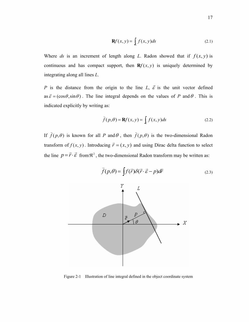
P is the distance from the origin to the line L, εr is the unit vector defined
as )sin,(cos θθε =r . The line integral depends on the values of P andθ . This is
indicated explicitly by writing as:
∫==L
dsyxfyxfpf ),(),(),( Rθ(
(2.2)
If ),( θpf(
is known for all P andθ , then ),( θpf(
is the two-dimensional Radon
transform of ),( yxf . Introducing ),( yxr =r and using Dirac delta function to select
the line εrr⋅= rp from 2ℜ , the two-dimensional Radon transform may be written as:
∫ −⋅= rdprrfpf rrrr()()(),( εδθ (2.3)
Figure 2-1 Illustration of line integral defined in the object coordinate system
18
The function ),( θpf(
is often referred to as a sinogram because the Radon transform
of an off-center point source is a sinusoid. One of the important properties of the
Radon transform is symmetry,
),(),( πθθ +−= pfpf((
(2.4)
One-dimensional Fourier transform of ),( θpf(
with respect to p is
∫ −= dpepfpf pj ωπω θθ 2),(),(
((F (2.5)
By using θθε sincos yxrp +=⋅=rr , and substituting ),( θpf
(with (2.3), one get
)sin,cos(),(
)sincos(),(),()sincos(2
2
θωθω
θθδθωθθπ
ωπω
Fdxdyeyxf
dpdxdyepyxyxfpfyxj
pj
=∫∫=
∫∫∫ −+=+−
−(F
(2.6)
Here, ),( 21 ωωF is the Fourier transform of the function ),( yxf . Thus the one-
dimensional Fourier transform of the projections ),( θpf(
is equivalent to the two-
dimensional Fourier transform of ),( yxf evaluated along the line described by
θωω tan12 = (i.e. a straight line at an angleθ ). This is what is called Fourier Central
Slice theorem. In a polar grid, we have:
)sin,cos(),( θωθωθω FP = (2.7)
in the Fourier space, ),( θωP has following property:
),(),( θωπθω −=+ PP (2.8)
This theorem reveals the relationship between the projection function and the object
function. It also suggests that a simple inversion formula is to take the one-
19
dimensional Fourier transform of the projection at an angleθ , “put it down” on the
line at an angle θ in the two-dimensional Fourier space and interpolate to the
Cartesian grid. Once this is done for all angles, reconstruct the image with a two-
dimensional inverse Fourier transform. In practice, however, this method was rarely
used since the interpolation-induced errors were large.
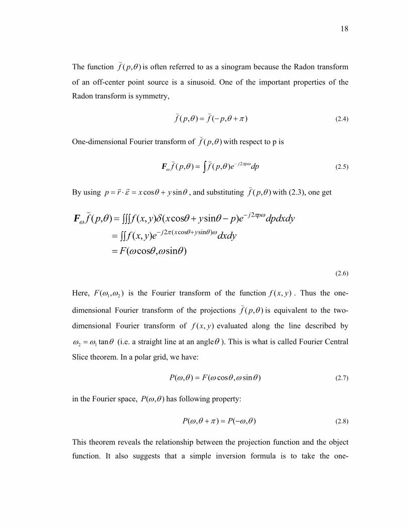
2.1.2 Three-dimensional RT and FCS theorem
The Three-dimensional Radon transform is related to the plane integral, which is
illustrated by Figure 2-2.
Figure 2-2 Illustrations of three-dimensional Radon transform defined in the object coordinate
system
The distance from the origin of the coordinate to the plane Π is p; εr is the unit
vector normal to the planeΠ , and is defined as )cos,sinsin,cos(sin θϕθϕθε =r . In
real space 3ℜ , the Radon transform of the real function )(rf r can be represented in
polar coordinates as,
20
∫ ∫ ∫ −⋅=−
∞π π
πϕθεδε
2
0
2
2 0)()(),( dpdpdprrfpf
rrrr( (2.9)
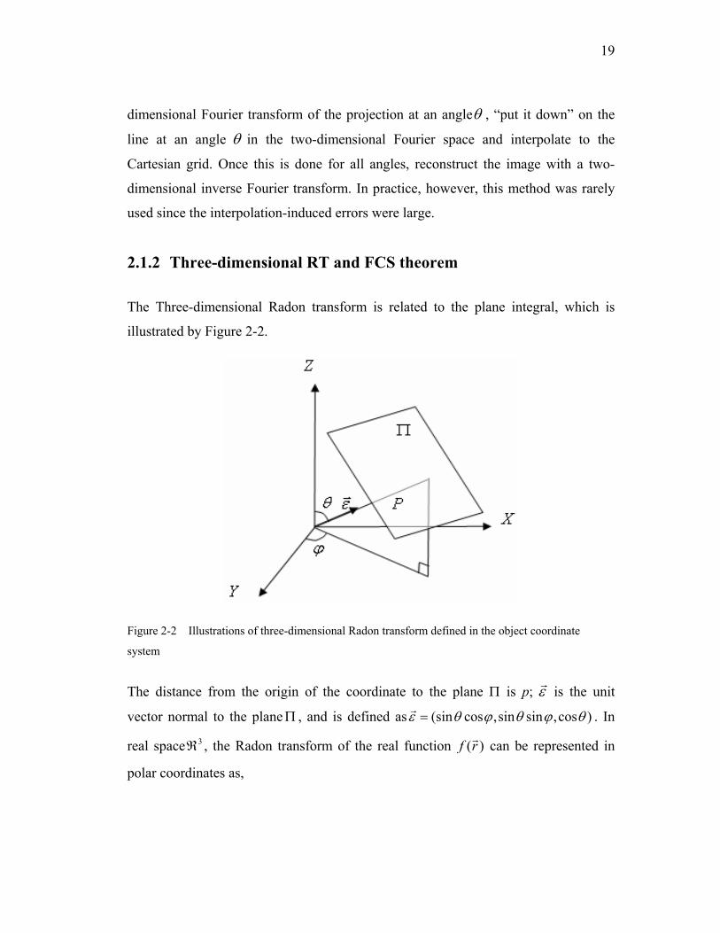
In 3D Radon space, the value of the plane integral represents a Radon point. The
distance from this point to the Radon space origin is p, and the same unit vector
εr determines the direction from the origin to this point. An array of parallel plane
integral specified by the same norm of εr and different distance of p with respect to
the origin constitute a radial line of Radon value passing through the origin. One-
dimensional Fourier transform of this radial Radon line is identical to the data along
the same line passing through the origin in the 3D Fourier space of the object
function )(rf r , as is illustrated by the Figure2-3. This is the 3D Fourier Central Slice
theorem.
Figure 2-3 Illustration of the 3D Fourier Central Slice Theorem
21
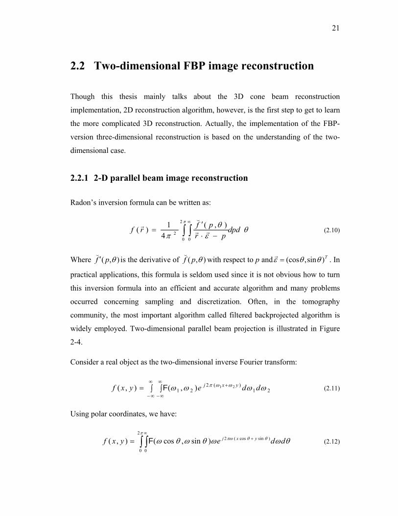
2.2 Two-dimensional FBP image reconstruction
Though this thesis mainly talks about the 3D cone beam reconstruction
implementation, 2D reconstruction algorithm, however, is the first step to get to learn
the more complicated 3D reconstruction. Actually, the implementation of the FBP-
version three-dimensional reconstruction is based on the understanding of the two-
dimensional case.
2.2.1 2-D parallel beam image reconstruction
Radon’s inversion formula can be written as:
θε
θπ
π
dpdpr
pfrf ∫ ∫∞
−⋅′
=2
0 02
),(4
1)( rr
(r
(2.10)
Where ),( θpf ′(
is the derivative of ),( θpf(
with respect to p and T)sin,(cos θθε =r . In
practical applications, this formula is seldom used since it is not obvious how to turn
this inversion formula into an efficient and accurate algorithm and many problems
occurred concerning sampling and discretization. Often, in the tomography
community, the most important algorithm called filtered backprojected algorithm is
widely employed. Two-dimensional parallel beam projection is illustrated in Figure
2-4.
Consider a real object as the two-dimensional inverse Fourier transform:
∫ ∫=∞
∞−
∞
∞−
+21
)(221
21),(),( ωωωω ωωπ ddeyxf yxjF (2.11)
Using polar coordinates, we have:
∫ ∫∞
+=π
θθπω θωωθωθω2
0 0
)sincos(2)sin,cos(),( ddeyxf yxjF (2.12)
22
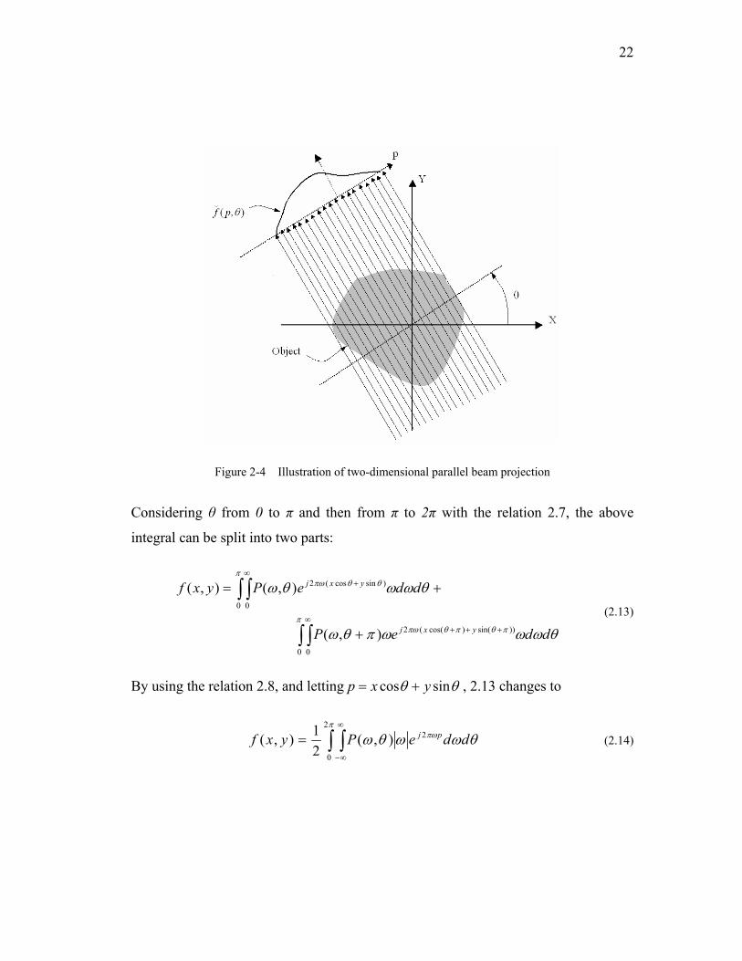
Figure 2-4 Illustration of two-dimensional parallel beam projection
Considering θ from 0 to π and then from π to 2π with the relation 2.7, the above
integral can be split into two parts:
∫ ∫
∫ ∫∞
+++
∞+
+
+=
ππθπθπω
πθθπω
θωωωπθω
θωωθω
0 0
))sin()cos((2
0 0
)sincos(2
),(
),(),(
ddeP
ddePyxf
yxj
yxj
(2.13)
By using the relation 2.8, and letting θθ sincos yxp += , 2.13 changes to
∫ ∫∞
∞−
=π
πω θωωθω2
0
2),(21),( ddePyxf pj (2.14)
23
),( θωP is the Fourier transform of the projection ),( θpf(
, ω , usually called the
ramp filter, is the modulation transfer function (MTF) of the filter in Fourier space.
The inner integral
∫∞
∞−
= ωωθωθ πω dePpQ pj2),(),( (2.15)
Where ),( θpQ is what we call ‘filtered projection’ on the projection angleθ . The
outer integral in 2.14 with respect to θ is the backprojection operation. In practical
application, this approach is expected to have problems with noise because the ramp
filter ω significantly amplifies any high frequency content in ),( θpQ . The
regularization necessary to enable acceptable reconstruction is to apply a low-pass
filter )(ωΩW to ωθω ),(P and find the filtered projections as:
∫∞
∞−ΩΩ = ωωωθωθ πω deWPpQ pj2)(),(),( (2.16)
Usually the Shepp-Logan, Hamming, Hanning, and cosine windows are employed to
represent )(ωΩW . So the reconstructed object is a band-limited reconstruction of the
original object. The final reconstruction formula becomes:
∫ ∫∞
∞−Ω=
ππω θωωωθω
2
0
2)(),(21),( ddeWPyxf pj)
(2.17)
This formula can also be written in terms of convolution:
∫ ∫∞
∞−
−−=π
θφθθ2
0
))cos((),(21),( dpdprhpfyxf
() (2.18)
Wherexyyxr 122 tan, −=+= φ , and )( ph is the impulse response of the
regularized filter.
24
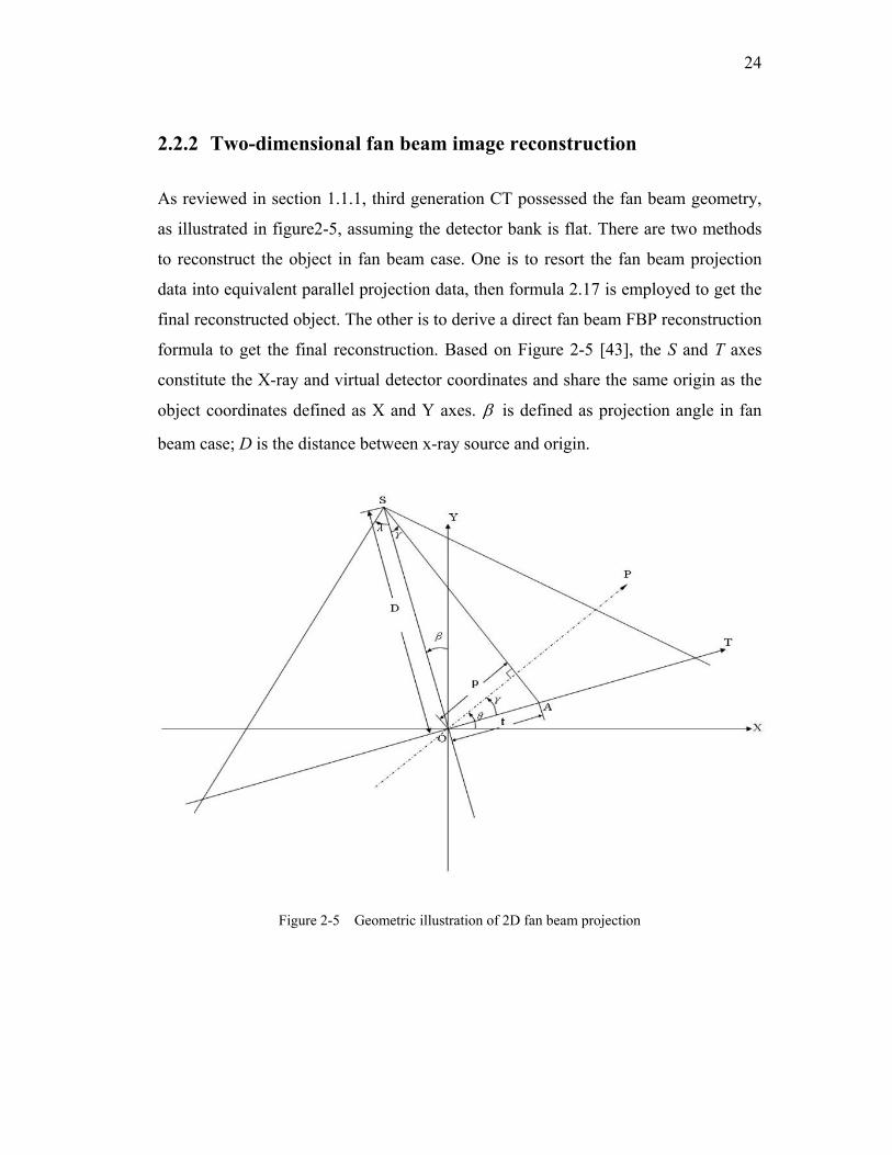
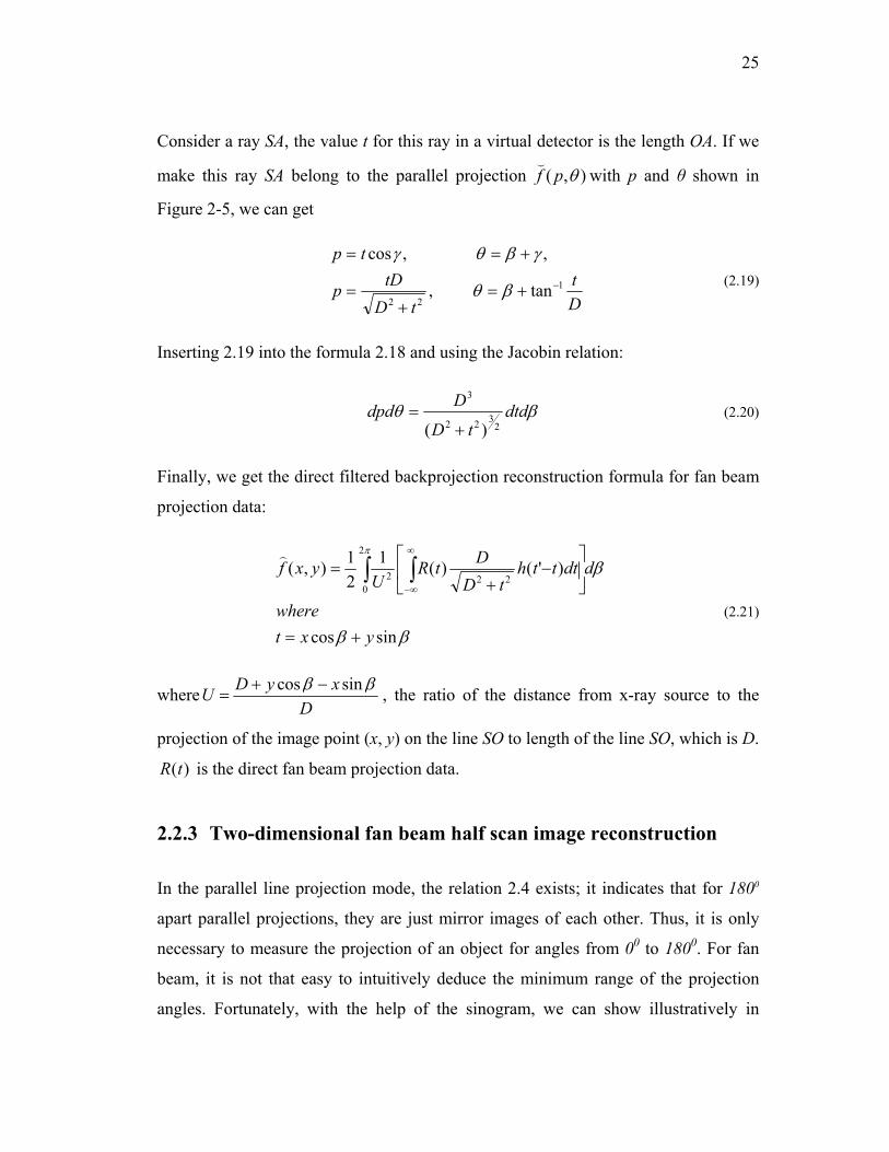
2.2.2 Two-dimensional fan beam image reconstruction
As reviewed in section 1.1.1, third generation CT possessed the fan beam geometry,
as illustrated in figure2-5, assuming the detector bank is flat. There are two methods
to reconstruct the object in fan beam case. One is to resort the fan beam projection
data into equivalent parallel projection data, then formula 2.17 is employed to get the
final reconstructed object. The other is to derive a direct fan beam FBP reconstruction
formula to get the final reconstruction. Based on Figure 2-5 [43], the S and T axes
constitute the X-ray and virtual detector coordinates and share the same origin as the
object coordinates defined as X and Y axes. β is defined as projection angle in fan
beam case; D is the distance between x-ray source and origin.
Figure 2-5 Geometric illustration of 2D fan beam projection
25
Consider a ray SA, the value t for this ray in a virtual detector is the length OA. If we
make this ray SA belong to the parallel projection ),( θpf(
with p and θ shown in
Figure 2-5, we can get
Dt
tDtDp
tp
1
22tan,
,,cos
−+=+
=
+==
βθ
γβθγ (2.19)
Inserting 2.19 into the formula 2.18 and using the Jacobin relation:
βθ dtdtD
Ddpd2
322
3
)( += (2.20)
Finally, we get the direct filtered backprojection reconstruction formula for fan beam
projection data:
ββ
βπ
sincos
)'()(121),(
2
0222
yxtwhere
ddttthtD
DtRU
yxf
+=
⎥⎦
⎤⎢⎣
⎡−
+= ∫ ∫
∞
∞−
)
(2.21)
whereD
xyDU ββ sincos −+= , the ratio of the distance from x-ray source to the
projection of the image point (x, y) on the line SO to length of the line SO, which is D.
)(tR is the direct fan beam projection data.
2.2.3 Two-dimensional fan beam half scan image reconstruction
In the parallel line projection mode, the relation 2.4 exists; it indicates that for 1800
apart parallel projections, they are just mirror images of each other. Thus, it is only
necessary to measure the projection of an object for angles from 00 to 1800. For fan
beam, it is not that easy to intuitively deduce the minimum range of the projection
angles. Fortunately, with the help of the sinogram, we can show illustratively in
26
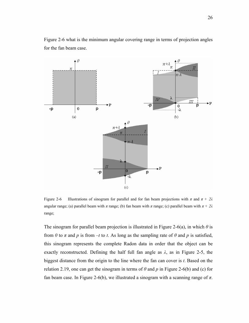
Figure 2-6 what is the minimum angular covering range in terms of projection angles
for the fan beam case.
Figure 2-6 Illustrations of sinogram for parallel and for fan beam projections with π and π + 2λ
angular range; (a) parallel beam with π range; (b) fan beam with π range; (c) parallel beam with π + 2λ
range;
The sinogram for parallel beam projection is illustrated in Figure 2-6(a), in which θ is
from 0 to π and p is from –t to t. As long as the sampling rate of θ and p is satisfied,
this sinogram represents the complete Radon data in order that the object can be
exactly reconstructed. Defining the half full fan angle as λ, as in Figure 2-5, the
biggest distance from the origin to the line where the fan can cover is t. Based on the
relation 2.19, one can get the sinogram in terms of θ and p in Figure 2-6(b) and (c) for
fan beam case. In Figure 2-6(b), we illustrated a sinogram with a scanning range of π.
27
Two black spots represent the x-ray starting and ending positions in terms of
projection angle β defined in Figure 2-5. The two regions marked as I and III are the
area in the Radon space where there is no measurement of the object. On the other
hand, the two gray shaded regions labeled as II and IV are the area in Radon space
where there are redundant measurements of the object. Compared with Figure 2-6(a),
the missing data in Radon space resulting from the fan beam scanning with a range of
π will cause an inexact and degraded image reconstruction. However, as we increase
the scanning range associated with the fan beam from π to π + 2λ, the empty area is
filled as Figure 2-6(c) illustrates. The gray shaded regions I and II represent the
redundant measurement of the object in Radon space. Usually, a weighing window
function is employed on the redundant projection data before filtering. In order to get
the more accurate reconstruction, a mathematically smoother window function that is
both continuous and has a continuous derivative at the boundary between single and
double sampled regions is employed along the P axis on the sinogram. Defining this
weighting function as )(γβw , it must satisfy
12
112
21
,2
,1)()(21
γγγβπβ
γγ ββ
−=−+=
=+ ww
(2.22)
By using the relation Dtarctan=γ , the weighting function )(γβw can be represented
as )(twβ . So the final FBP version of the half scan fan beam is:
ββ
βλπ
β
sincos
)'()()(1),(2
0222
yxtwhere
ddttthtD
DtRtwU
yxf
+=
⎭⎬⎫
⎩⎨⎧
−⎥⎦
⎤⎢⎣
⎡
+= ∫ ∫
+ ∞
∞−
)
(2.23)
The weighting of the projection data must be done before the filtering. Otherwise, the
reconstruction will have some obvious streak artifacts.
28
2.3 Three-dimensional FBP image reconstruction
Traditionally, stacking a series of two-dimensional cross sectional images on top of
each other is the only method to make three-dimensional image. However this
stacking technology results in several limitations such as poor axial resolution of the
reconstruction and long scanning time. Fortunately, these limitations are eliminated
by use of the three-dimensional cone beam geometry and direct reconstruction of
three-dimensional images. Based on the scanning trajectory, cone beam
reconstruction can be roughly divided into two categories, one is employed with only
a circular scan and approximate algorithms were developed to reconstruct a 3D image;
the other is employed with non-planar scanning orbits in which exact analytical
inversion formulas were developed for image reconstruction. Of course, the exact
inversion formula can also be adopted to reconstruct the object in circular scan.
Though the iterative algorithms are important in dealing with the incomplete data,
their application in practical medical CT diagnosing is very limited. So, we are not
going to touch it in this dissertation.
2.3.1 The data sufficient condition with cone beam reconstruction
Using the three-dimensional Radon transform (formula 2.9), assuming that the
support of the object in three-dimensional Radon space is a ball with the radius of R,
and if all the information inside the Radon ball were known, then the object
)(rf r would theoretically be reconstructed using the three-dimensional inverse Radon
transform
∫ ∫−
∂∂
−=2
2
2
02
2
2 sin),(8
1)(π
π
π
θϕθεπ
ddpfP
rf r(r (2.24)
This is a theoretically exact reconstruction. Each point in the Radon domain
represents a plane integral in the object space and this plane must have at least an x-
29
ray source. Thus, it is intuitive to state that in order to get the exact, in other words,
artifact-free reconstruction, the scanning trajectory must satisfy the condition that on
every plane intersecting the object there exists a vertex. This is the Data Sufficient
Condition (DSC) for exact cone beam reconstruction resulting from the fundamental
work by Tuy, Smith and Grangeat [44-47]. Based on the reformulation of the
Grangeat’s work by Axelsson and Danielsson [48-49], the DSC can be obtained from
another point of view. In Figure 2-7, a Radon shell is defined with SO as the diameter
(where S and O denote a source position and the reconstruction system origin,
respectively). Consider a Radon point εrp on the Radon shell and on the plane SL1L2.
The normal of this plane is εr . The Radon value at εrp can be calculated by
integrating the object function ),,( zyxf over the plane SL1L2. Using the polar
coordinate λ and r , one obtain
∫ ∫=−
∞2
2 0),,(),(
π
πλλεε rdrdrpfpf
rr( (2.25)
However, the x-ray projection data in this plane is the line integral
∫∞
=0
),,(),,( drrpfpX λεαεrr
(2.26)
Apparently, the factor r in formula 2.25 caused the problem in connecting the Radon
transform ),( εr(
pf to the x-ray cone beam projection data ),,( αεrpX . Fortunately, by
performing the following manipulation [47], the relationship between
),( εr(
pf and ),,( αεrpX can be established as
30
λλαε
α
λλ
λεα
λλεε
π
π
π
π
π
π
dpXdd
ddrrpfdd
rdrdrpfdpd
dppfd
∫
∫ ∫
∫ ∫
−
−
∞
−
∞
=
⎥⎦
⎤⎢⎣
⎡=
=
2
2
2
2 0
2
2 0
cos),,(
cos1),,(
),,(),(
r
r
rr(
(2.27)
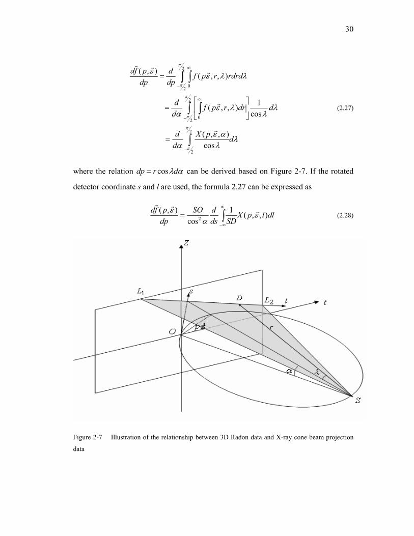
where the relation αλdrdp cos= can be derived based on Figure 2-7. If the rotated
detector coordinate s and l are used, the formula 2.27 can be expressed as
dllpXSDds
dSOdppfd ),,(1
cos),(
2 εα
ε rr(
∫∞
∞−
= (2.28)
Figure 2-7 Illustration of the relationship between 3D Radon data and X-ray cone beam projection
data
31
Therefore, in order to compute the radial derivative of ),( εr(
pf , there must be at least
one x-ray source position on the plane through ),( εrp . This immediately leads to the
DSC for exact cone-beam reconstruction. There was a good thorough review of DSC
in [50].
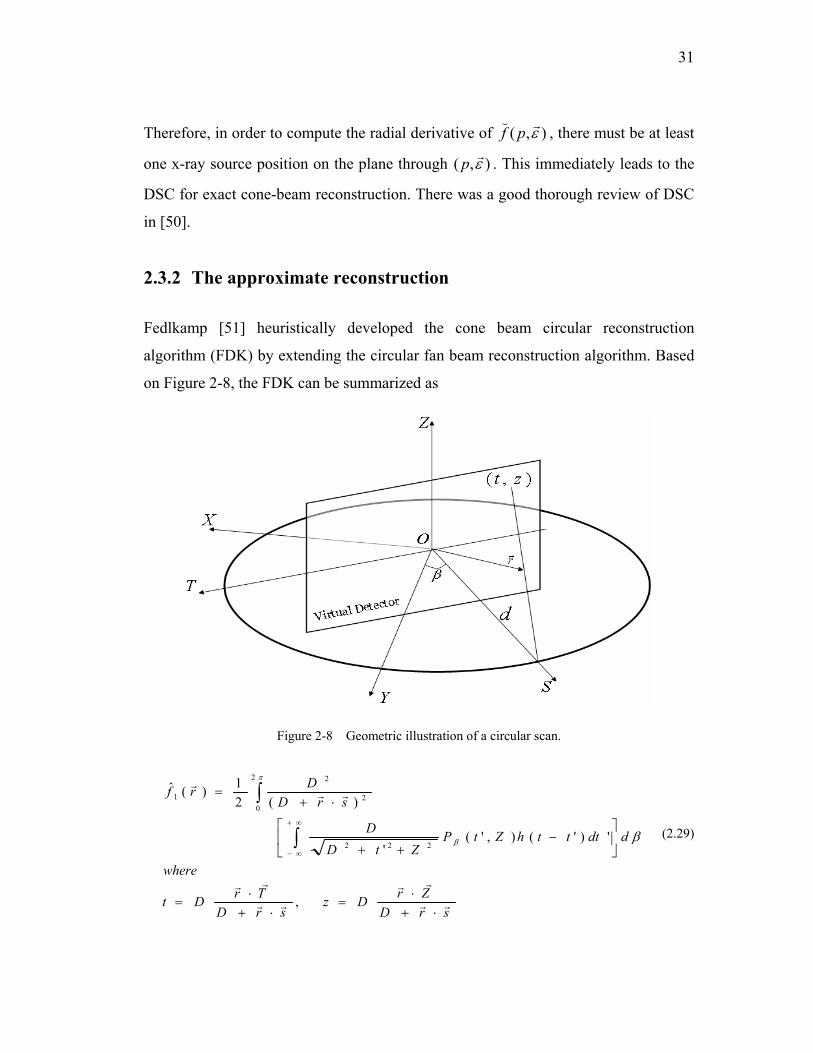
2.3.2 The approximate reconstruction
Fedlkamp [51] heuristically developed the cone beam circular reconstruction
algorithm (FDK) by extending the circular fan beam reconstruction algorithm. Based
on Figure 2-8, the FDK can be summarized as
Figure 2-8 Geometric illustration of a circular scan.
srDZrDz
srDTrDt
where
ddttthZtPZtD
D
srDDrf
rr
rr
rr
rr
rrr
⋅+⋅
=⋅+
⋅=
⎥⎦
⎤⎢⎣
⎡−
++
⋅+=
∫
∫∞+
∞−
,
')'(),'('
)(21)(ˆ
222
2
02
2
1
ββ
π
(2.29)
32
Formula 2.29 has the same frame structure as the formula 2.21: one-dimensional
filtering along T axis and backprojection summation in terms of the projection angle β.
),( ZtPβ is the cone beam projection on the two-dimensional detector. FDK is by far
the most employed algorithm in practical cone beam tomography reconstruction due
to the computational efficiency, better spatial/contrast resolution and temporal
resolution, etc.
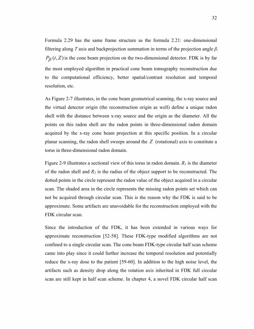
As Figure 2-7 illustrates, in the cone beam geometrical scanning, the x-ray source and
the virtual detector origin (the reconstruction origin as well) define a unique radon
shell with the distance between x-ray source and the origin as the diameter. All the
points on this radon shell are the radon points in three-dimensional radon domain
acquired by the x-ray cone beam projection at this specific position. In a circular
planar scanning, the radon shell sweeps around the Z (rotational) axis to constitute a
torus in three-dimensional radon domain.
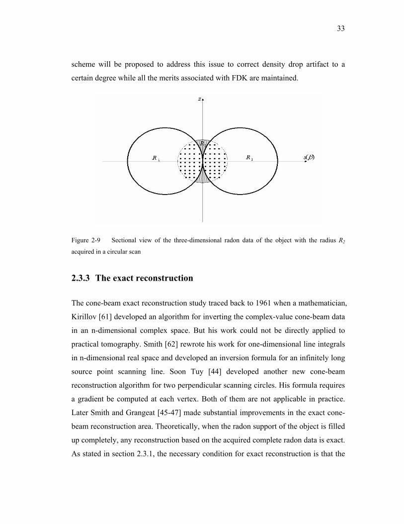
Figure 2-9 illustrates a sectional view of this torus in radon domain. R1 is the diameter
of the radon shell and R2 is the radius of the object support to be reconstructed. The
dotted points in the circle represent the radon value of the object acquired in a circular
scan. The shaded area in the circle represents the missing radon points set which can
not be acquired through circular scan. This is the reason why the FDK is said to be
approximate. Some artifacts are unavoidable for the reconstruction employed with the
FDK circular scan.
Since the introduction of the FDK, it has been extended in various ways for
approximate reconstruction [52-58]. These FDK-type modified algorithms are not
confined to a single circular scan. The cone beam FDK-type circular half scan scheme
came into play since it could further increase the temporal resolution and potentially
reduce the x-ray dose to the patient [59-60]. In addition to the high noise level, the
artifacts such as density drop along the rotation axis inherited in FDK full circular
scan are still kept in half scan scheme. In chapter 4, a novel FDK circular half scan
33
scheme will be proposed to address this issue to correct density drop artifact to a
certain degree while all the merits associated with FDK are maintained.
Figure 2-9 Sectional view of the three-dimensional radon data of the object with the radius R2
acquired in a circular scan
2.3.3 The exact reconstruction
The cone-beam exact reconstruction study traced back to 1961 when a mathematician,
Kirillov [61] developed an algorithm for inverting the complex-value cone-beam data
in an n-dimensional complex space. But his work could not be directly applied to
practical tomography. Smith [62] rewrote his work for one-dimensional line integrals
in n-dimensional real space and developed an inversion formula for an infinitely long
source point scanning line. Soon Tuy [44] developed another new cone-beam
reconstruction algorithm for two perpendicular scanning circles. His formula requires
a gradient be computed at each vertex. Both of them are not applicable in practice.
Later Smith and Grangeat [45-47] made substantial improvements in the exact cone-
beam reconstruction area. Theoretically, when the radon support of the object is filled
up completely, any reconstruction based on the acquired complete radon data is exact.
As stated in section 2.3.1, the necessary condition for exact reconstruction is that the
34
scanning trajectory must satisfy the DSC. Based on the Smith and Grangeat’s work,
one kind of exact reconstruction methods using the 3D Fourier central slice theorem
was derived [48-49, 63-65]. This method is computationally efficient but with high
image noise and ring artifacts. Another set of methods is based on the radon inversion
formula and is formulated in the framework of filtered backprojection (FBP). This
method can further be classified into two sub-methods. The first group is a unified
method which means only one algorithm is employed to conduct the exact
reconstruction [47, 66-70]; the second group is what is usually called the composite
or hybrid method which means two or more trajectories are used to get the complete
radon data; then, corresponding algorithms are used to conduct the respective
reconstruction. Their results are finally added together to get the exact reconstruction
[71-76]. The scanning trajectory associated with the first group can be either like a
helix curve or saddle curve to satisfy the DSC. Please note that the DSC discussed in
section 2.3.1 only deals with the short object case, which means the X-ray covers the
whole object during the scan. In practical application, longitudinal truncation is
commonly encountered. In order to make the exact reconstruction for a volume of
interest (VOI), Grangeat [77] proposed another DSC associated with his formula
framework, which later was refined by Clack and Defris [78]. This makes exact
reconstruction of the VOI inside the object available when the radon support of this
VOI is filled up completely. But the extended DSC proposed by Kudo and Saito [79-
80] is more appropriate for the source orbit of a circular sub-orbit and supplemental
non-circular sub-orbit.
Due to the continuous quest for the accurate image reconstruction in helical cone-
beam tomography, Katsevich made a breakthrough in developing the first exact cone
beam reconstruction algorithms with shift-invariant FBP structure [81-82]. Later, Zou
and Pan reformatted the Katsevich’s formula by interchanging the order of the
backprojection and Hilbert filtering, and proposing what they called backprojection
filtration (BPF) exact reconstruction algorithm [83]. The implementation of these
algorithms is based on the recognition of the π-line segment as long as the DSC is
35
satisfied and non-redundant data is acquired. In terms of operational and
computational efficiency, BPF is inferior to FBP. But BPF approach is much more
flexible in handling truncated data compared with FBP. Katsevich later generalized
his methods for general scanning trajectories based on radon inversion formula [84].
Based on his work, various methods that collect cone beam data from general
scanning trajectories have been developed [85-90] and implemented [91].
36
Chapter 3 Circle plus partial helical line segment
scan with Cone Beam Breast CT
(CBBCT)
3.1 The development of cone beam breast CT
Breast cancer imaging has improved over the last decade with higher and more
uniform quality standards for mammography, as well as through the increasing use of
sonography and magnetic resonance imaging as the adjunct tools. Mammography is
still the only screening tool to detect breast cancer for asymptomatic women. Due to
the limitations associated with the aforementioned techniques, such as imaging of the
overlapping structure with mammography, technician dependent lack of ability to
detect calcifications with ultrasound, and low specificity; and/or poor detection of the
tiny calcium deposits with MRI, there remains an endeavor to explore new ways to
better detect breast cancer. Recently, one of the most exciting ways to detect breast
cancer is cone beam breast CT (CBBCT) technology [92-94]. It is based on a flat
panel detector and with only one circular rotation or some other closed scanning orbit.
It can provide the three-dimensional density distribution of the breast greatly
eliminating the imaging problem of the structure overlap seen in mammography and
enhancing the contrast resolution. It has been shown that the average glandular doses
of CBBCT is equivalent to or lower than mammography [95-96]. So, this technology
37
has the potential to possibly replace mammography for breast cancer screening and
diagnosis.
Among all CBBCT technologies, FDK [51, 58] algorithm-based circular scanning
possesses the following advantages: a stable and simple mechanical configuration;
motion artifacts reduction; computation efficiency among others. However, since a
single circular source trajectory does not satisfy the DSC and CBCT has a relatively
large cone angle, the FDK algorithm will unavoidably induce some artifacts such as
an intensity drop along the rotation axis and geometric distortion around the nipple
area. In order to overcome these cone beam artifacts, we propose the circle plus
partial helical line (CHL) scanning scheme. Based on the idea that by partially filling
the object support in the Radon domain (i.e. the well-known torus in 3-D Radon
domain) where the circular scanning does not touch through the additional scanning
path (such as a helical line path), we can acquire more information than from just a
single circular scan. This combined scanning scheme will result in better image
quality of the reconstructed object. The idea behind the partial helical scan is to
improve the image quality while not exposing the patient to too much radiation. In
order to maintain computation efficiency, a filtered backprojection method is
employed for the reconstruction part associated with a partial helical scan.
Recently, Katsevich [99] proposed a circle plus general curve scan algorithm, which
is of FBP type. It is an exact shift-invariant algorithm and computationally efficient.
The requirements for this additional scanning are that first, this additional general
curve has to be a piece-wise smooth curve (i.e. a straight line or helix); second, during
this additional scanning, the circle trajectory must find its projection on the detector
as it is seen from the X-ray source. General CT scanner and C-arm can easily meet
the requirements and exact ROI reconstructions can be achieved by employing this
algorithm. In case of CBBCT, since the scanner possesses a half cone geometry
covering the whole detector, and it is better to keep the X-ray collimation fixed
during additional non-circular scanning to reduce the system complexity, the second
38
requirement associated with aforementioned Katsevich algorithm is hard to meet.
Based on the special geometric requirement of CBBCT, the proposed helical line part
will be reconstructed using a shift-variant filtered-backprojection [72]. Under less
restrictive conditions, Katsevich type reconstruction is conducted along a straight line
scanning in numerical simulation. The hybrid reconstruction method is adopted for
both cases. For the proposed CHL scheme, the reconstruction is composed of three
parts: FDK term for circle [51]; Hui’s term for circle scan[97]; and a shift-variant
FBP term for helical line scan; whereas for circle plus straight line (CL) scheme, the
reconstruction is composed of two terms, FDK term for circle scan, and Katsevich
term [90] for straight line scan. FDK is used for both cases for the circle part due to
the better computational efficiency and spatial resolution [100]. Results from both
cases are compared and discussed. Overall, computer simulations based on the
prototype CBBCT system parameters and experimental studies with a breast phantom
verified that the proposed CHL scheme outperforms the FDK-based single circular
scan scheme.
3.2 The circle plus partial helical line scanning
(CHL)
3.2.1 Data acquisition analysis in terms of Radon domain
It is well known that a single circular cone beam scan does not provide complete
information for an exact reconstruction. This can be appreciated by the three-
dimensional Radon transform of the object function )(rf r , which is mathematically
shown as:
∫ −⋅⋅= rdrrfRf rrrrr)()()( ρεδερ (3.1)
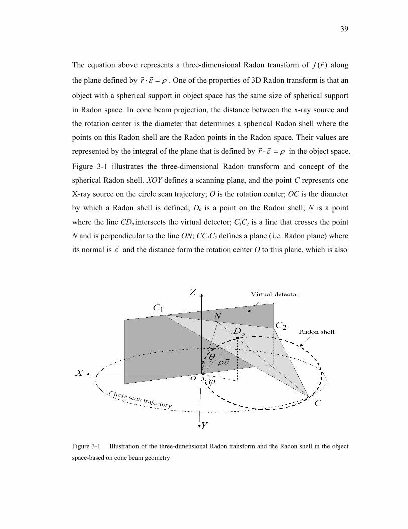
39
The equation above represents a three-dimensional Radon transform of )(rf r along
the plane defined by ρε =⋅rrr . One of the properties of 3D Radon transform is that an
object with a spherical support in object space has the same size of spherical support
in Radon space. In cone beam projection, the distance between the x-ray source and
the rotation center is the diameter that determines a spherical Radon shell where the
points on this Radon shell are the Radon points in the Radon space. Their values are
represented by the integral of the plane that is defined by ρε =⋅rrr in the object space.
Figure 3-1 illustrates the three-dimensional Radon transform and concept of the
spherical Radon shell. XOY defines a scanning plane, and the point C represents one
X-ray source on the circle scan trajectory; O is the rotation center; OC is the diameter
by which a Radon shell is defined; D0 is a point on the Radon shell; N is a point
where the line CD0 intersects the virtual detector; C1C2 is a line that crosses the point
N and is perpendicular to the line ON; CC1C2 defines a plane (i.e. Radon plane) where
its normal is εr and the distance form the rotation center O to this plane, which is also
Figure 3-1 Illustration of the three-dimensional Radon transform and the Radon shell in the object
space-based on cone beam geometry
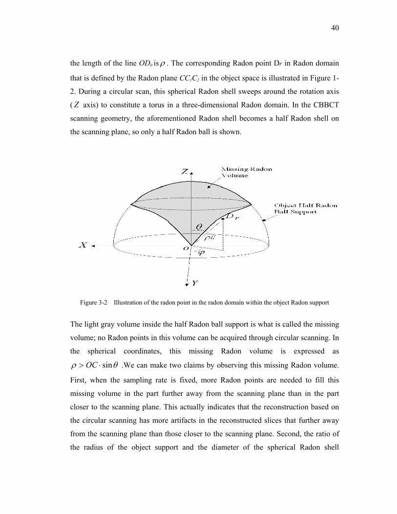
40
the length of the line OD0 is ρ . The corresponding Radon point Dr in Radon domain
that is defined by the Radon plane CC1C2 in the object space is illustrated in Figure 1-
2. During a circular scan, this spherical Radon shell sweeps around the rotation axis
( Z axis) to constitute a torus in a three-dimensional Radon domain. In the CBBCT
scanning geometry, the aforementioned Radon shell becomes a half Radon shell on
the scanning plane, so only a half Radon ball is shown.
Figure 3-2 Illustration of the radon point in the radon domain within the object Radon support
The light gray volume inside the half Radon ball support is what is called the missing
volume; no Radon points in this volume can be acquired through circular scanning. In
the spherical coordinates, this missing Radon volume is expressed as
θρ sin⋅> OC .We can make two claims by observing this missing Radon volume.
First, when the sampling rate is fixed, more Radon points are needed to fill this
missing volume in the part further away from the scanning plane than in the part
closer to the scanning plane. This actually indicates that the reconstruction based on
the circular scanning has more artifacts in the reconstructed slices that further away
from the scanning plane than those closer to the scanning plane. Second, the ratio of
the radius of the object support and the diameter of the spherical Radon shell
41
determines the size of the missed Radon data volume, which results in the
reconstructed object that is closer to or farther away from the exact reconstruction.
With the diameter (i.e. the distance between the x-ray source and the rotation center)
of the Radon shell fixed, the smaller the breast, the better the reconstructed image; the
bigger the breast, the worse the reconstructed image in terms of artifacts.
According to Chen and Ning [92], when the distance between the nipple and the chest
wall (HCN) is equal or less than 12 cm, (This HCN corresponds to the half-cone
angle of 8 degrees based on their scanning geometry), the circular-based modified
FDK (MFDK) [97] (which is the addition of first two terms in CHL scheme) still
provides clinically acceptable reconstructed images. However, as the HCN increases
to the size bigger than 12 cm, artifacts such as density drop and geometrical
deformation are more noticeable in the reconstructed images based on a single
circular scanning. An additional scanning trajectory should be added to fill the
missing Radon data volume in order to produce clinically acceptable images. Based
on the analysis in the previous paragraphs, the filling of the missing Radon volume
does not need to be complete. In other words, only part of the missing Radon volume
needs to be filled to correct, to a certain degree, the artifacts associated with a single
circle scan. In practical CBCT imaging, this missed volume is actually a small portion
in the half ball Radon support of the object. The sampling rate of Radon data within
this volume does not need to be as high as it does in the volume acquired through a
circular scan. These realizations do not require too much extra X-ray exposure by
introducing an auxiliary scanning trajectory and improve image quality to a certain
degree.
There are a couple of proposed ‘circle plus’ trajectories [67, 71-76, 101]. Due to the
special geometrical configuration of the CBBCT, the circle plus arc is not applicable.
However, the CL seems to be applicable. For ease of operation and in order to avoid
unnecessary extra X-ray exposure, the x-ray collimation associated with the circle
scan must be kept for line scan trajectory. The line-scan trajectory is described
42
as ),,0()( lmlL =φ , where m is a constant in the Y-axis, and l is a variable along the Z-
axis representing the line scan x-ray shot position. Based on the illustration from
Figure 3-1, we can see that only a half Radon shell associated with each X-ray
position during line scan can be defined and it is tangential to the XOZ plane. In
Figure 3-2, the filling of the Radon data from this line-scan can only be added in half
of the missing Radon volume separated by the XOZ plane. Since the missing Radon
volume is symmetrical around the rotation axis (Z axis), this unsymmetrical filling of
the Radon data in terms of projection angle in the missing Radon volume may not
achieve the best reconstruction result. By taking advantage of the CBBCT circular
scanning feature, one way to combat this unsymmetrical filling is to lower down the
x-ray tube and detector while simultaneously rotating them around the breast to
achieve an approximate symmetrical filling of the Radon data in the missing Radon
volume. It is like the helical scan but with sparse x-ray shoots at the position
described as ),sin,cos(),( nnnnnHL lDDl βββφ = ; D is the distance from the x-ray
tube to the rotation center; nl is the position along the Z axis described as
lnlln Δ−+= )1(0 , where 0l is the starting position along the Z axis for this partial
helical scan, n is number of shoots; lΔ is the line increment along the Z axis; β is the
projection angle described as ββ Δ−= )1(nn ; βΔ is the projection angle increment in the
unit of radians. The Radon data acquired through this scanning trajectory can fill the
part of this missing Radon volume. Thus the result is not an exact reconstruction. The
key point here is to introduce the additional scanning trajectory to correct to a certain
degree the reconstruction artifacts associated with a single circular scan.
Since Katsevich’s algorithm is intriguing in terms of mathematic exactness and shift-
invariant filtering, a CL scanning is also conducted in numerical simulation based on
Katsevich’s concept under the less restrictive conditions. During the line scanning,
the detector is always fixed at the position where circle scan is conducted, and the X-
ray collimation is varied to make sure that X-ray illumination always covers the
whole detector as it moves along the line trajectory. In this way, the missing radon
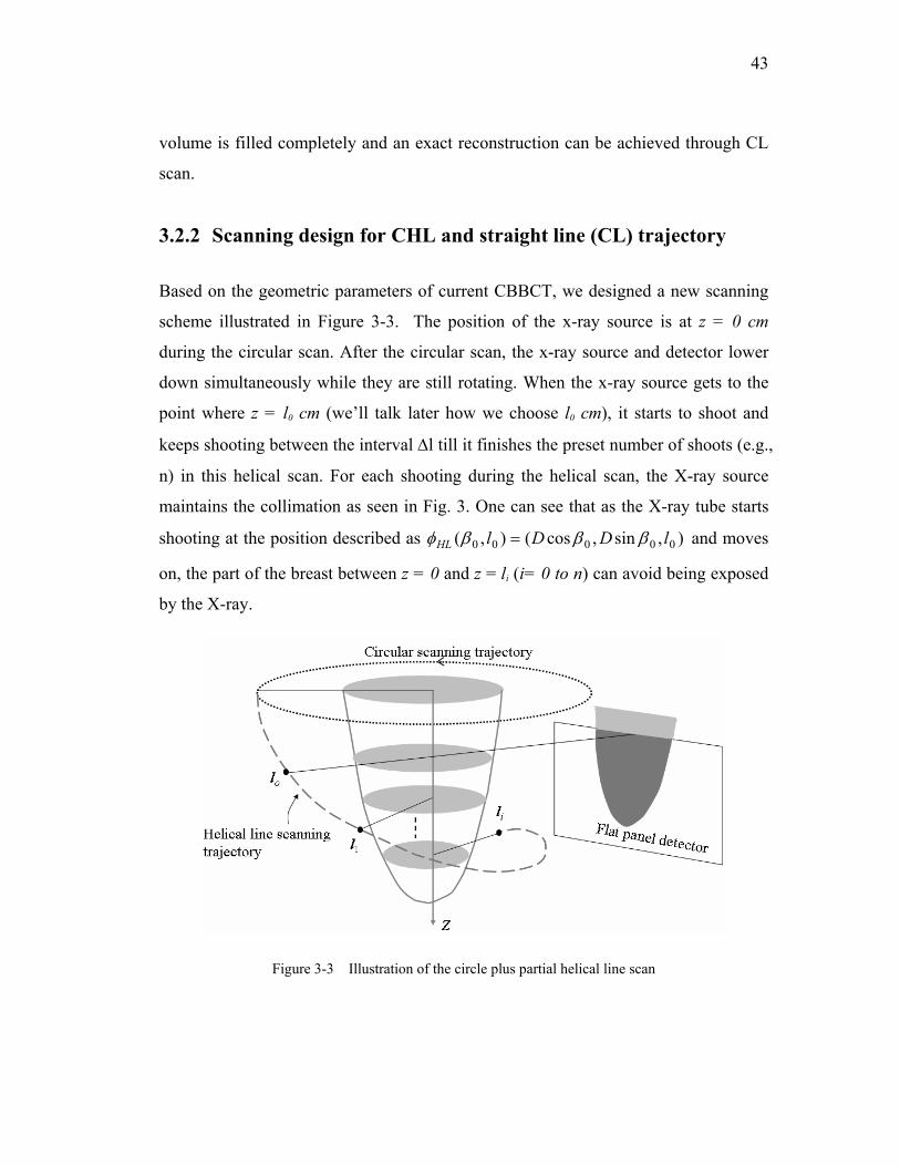
43
volume is filled completely and an exact reconstruction can be achieved through CL
scan.
3.2.2 Scanning design for CHL and straight line (CL) trajectory
Based on the geometric parameters of current CBBCT, we designed a new scanning
scheme illustrated in Figure 3-3. The position of the x-ray source is at z = 0 cm
during the circular scan. After the circular scan, the x-ray source and detector lower
down simultaneously while they are still rotating. When the x-ray source gets to the
point where z = l0 cm (we’ll talk later how we choose l0 cm), it starts to shoot and
keeps shooting between the interval Δl till it finishes the preset number of shoots (e.g.,
n) in this helical scan. For each shooting during the helical scan, the X-ray source
maintains the collimation as seen in Fig. 3. One can see that as the X-ray tube starts
shooting at the position described as ),sin,cos(),( 00000 lDDlHL βββφ = and moves
on, the part of the breast between z = 0 and z = li (i= 0 to n) can avoid being exposed
by the X-ray.
Figure 3-3 Illustration of the circle plus partial helical line scan
44
The projection angles associated with partial helical scans are uniformly distributed
within 2π range. There are 32 and 64 shoot points during helical scans that uniformly
cover the angular range of 2π, and the movement in the Z direction is from 49 mm to
121 mm with the increment interval of 2.34 and 1.15 mm based on the size of the
simulated breast phantom. The reason we chose to starting position at Z = 49 mm for
partial helical line scan is because we found that based on our simulated scanning
geometrical parameter, the attenuation coefficient drop in the regular circular scan
started approximately at Z = 49 mm.
Some of the Radon data points acquired from this additional scanning trajectory can
still be acquired through a circular scan. This is what is called redundant sampling
points in the Radon domain, and can efficiently be eliminated by the redundant
window function. The geometric setup of the collimator during the partial helical
scanning, as shown in Figure 3-3, can avoid the redundant sampling in the missing
volume in the Radon domain within the shooting points in a helical trajectory. Since
the collimation during partial helical scanning unavoidably encounters the
longitudinal truncation, a geometric dependent truncation window function has to be
used to handle this case to remove the incorrect Radon data.
In line scan case, as Figure 3-4 shows, the virtual detector length along the circular
rotation axis is W. Those little black dots represent the X-ray source at different
position in the line scan. During the line scan, the detector is fixed, the collimation of
the X-ray is adaptively changed to cover the whole detector, and the length of this
scanning line is 2W. The circle trajectory can always be projected onto the detector as
it is seen from the X-ray source during the straight line scanning enabling us to use
Katsevich’s algorithm to do the reconstruction for this line part.
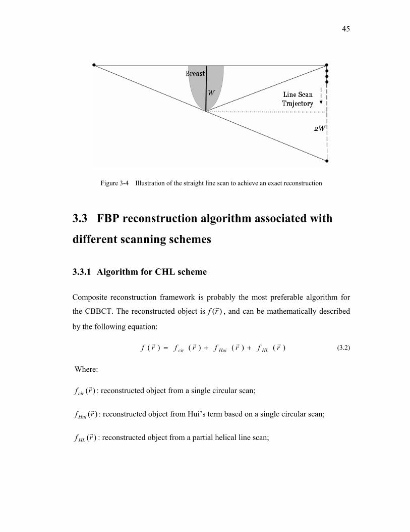
45
Figure 3-4 Illustration of the straight line scan to achieve an exact reconstruction
3.3 FBP reconstruction algorithm associated with
different scanning schemes
3.3.1 Algorithm for CHL scheme
Composite reconstruction framework is probably the most preferable algorithm for
the CBBCT. The reconstructed object is )(rf r , and can be mathematically described
by the following equation:
)()()()( rfrfrfrf HLHuicirrrrr
++= (3.2)
Where:
)(rfcirr : reconstructed object from a single circular scan;
)(rf Huir : reconstructed object from Hui’s term based on a single circular scan;
)(rf HLr : reconstructed object from a partial helical line scan;
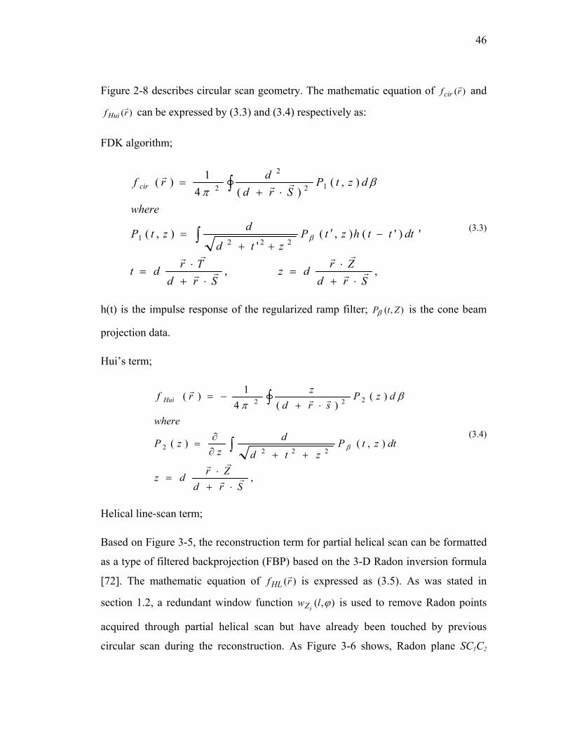
46
Figure 2-8 describes circular scan geometry. The mathematic equation of )(rf cirr and
)(rf Huir can be expressed by (3.3) and (3.4) respectively as:
FDK algorithm;
,,
')'(),('
),(
),()(4
1)(
2221
12
2
2
SrdZrdz
SrdTrdt
dttthztPztd
dztP
where
dztPSrd
drf cir
rr
rrrr
rr
rrr
⋅+⋅
=⋅+
⋅=
−′++
=
⋅+=
∫
∫
β
βπ
(3.3)
h(t) is the impulse response of the regularized ramp filter; ),( ZtPβ is the cone beam
projection data.
Hui’s term;
,
),()(
)()(4
1)(
2222
222
SrdZrdz
dtztPztd
dz
zP
where
dzPsrd
zrf Hui
rr
rr
rrr
⋅+⋅
=
++∂∂
=
⋅+−=
∫
∫
β
βπ
(3.4)
Helical line-scan term;
Based on Figure 3-5, the reconstruction term for partial helical scan can be formatted
as a type of filtered backprojection (FBP) based on the 3-D Radon inversion formula
[72]. The mathematic equation of )(rf HLr is expressed as (3.5). As was stated in
section 1.2, a redundant window function ),( ϕlwiZ is used to remove Radon points
acquired through partial helical scan but have already been touched by previous
circular scan during the reconstruction. As Figure 3-6 shows, Radon plane SC1C2
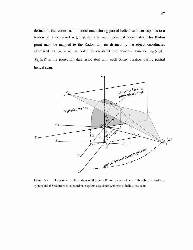
47
defined in the reconstruction coordinates during partial helical scan corresponds to a
Radon point expressed as ),,( θφρ ′ in terms of spherical coordinates. This Radon
point must be mapped to the Radon domain defined by the object coordinates
expressed as ),,( θφρ in order to construct the window function ),( ϕlwiZ .
),( ZtPiZ is the projection data associated with each X-ray position during partial
helical scan.
Figure 3-5 The geometric illustration of the same Radon value defined in the object coordinate
system and the reconstruction coordinate system associated with partial helical line scan
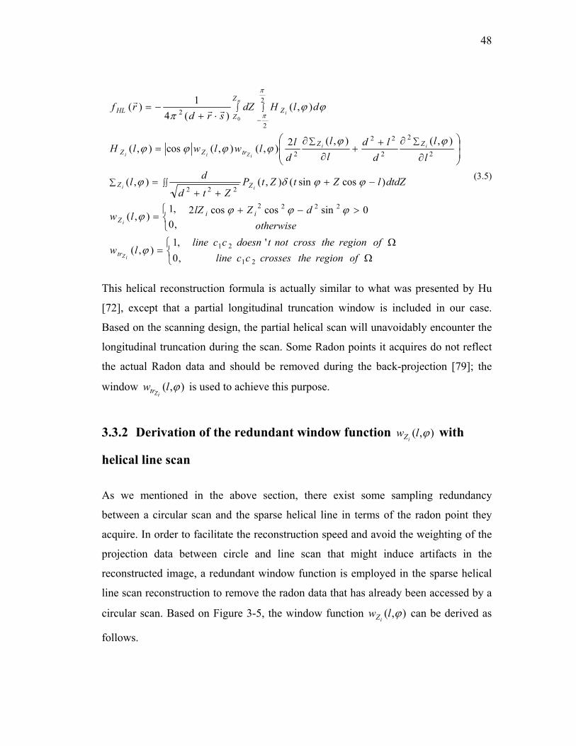
48
ΩΩ
⎩⎨⎧
=
>−+
⎩⎨⎧
=
−+++
=
⎟⎟⎠
⎞⎜⎜⎝
⎛
∂
∂++
∂∂
=
⋅+−=
∫∫∑
∑∑
∫∫−
ofregionthecrossescclineofregionthecrossnottdoesnccline
lw
otherwisedZlZlw
dtdZlZtZtPZtd
dl
ll
dld
ll
dllwlwlH
dlHdZsrd
rf
iZ
i
ii
ii
iZii
i
n
tr
iiZ
ZZ
ZZtrZZ
Z
Z
ZHL
21
21
2222
222
2
2
2
22
2
2
2
2
',0,1
),(
0sincoscos2,0,1
),(
)cossin(),(),(
),(),(2),(),(cos),(
),()(4
1)(0
ϕ
ϕϕϕϕ
ϕϕδϕ
ϕϕϕϕϕϕ
ϕϕπ
π
πrr
r
(3.5)
This helical reconstruction formula is actually similar to what was presented by Hu
[72], except that a partial longitudinal truncation window is included in our case.
Based on the scanning design, the partial helical scan will unavoidably encounter the
longitudinal truncation during the scan. Some Radon points it acquires do not reflect
the actual Radon data and should be removed during the back-projection [79]; the
window ),( ϕlwiZtr is used to achieve this purpose.
3.3.2 Derivation of the redundant window function ),( ϕlwiZ with
helical line scan
As we mentioned in the above section, there exist some sampling redundancy
between a circular scan and the sparse helical line in terms of the radon point they
acquire. In order to facilitate the reconstruction speed and avoid the weighting of the
projection data between circle and line scan that might induce artifacts in the
reconstructed image, a redundant window function is employed in the sparse helical
line scan reconstruction to remove the radon data that has already been accessed by a
circular scan. Based on Figure 3-5, the window function ),( ϕlwiZ can be derived as
follows.
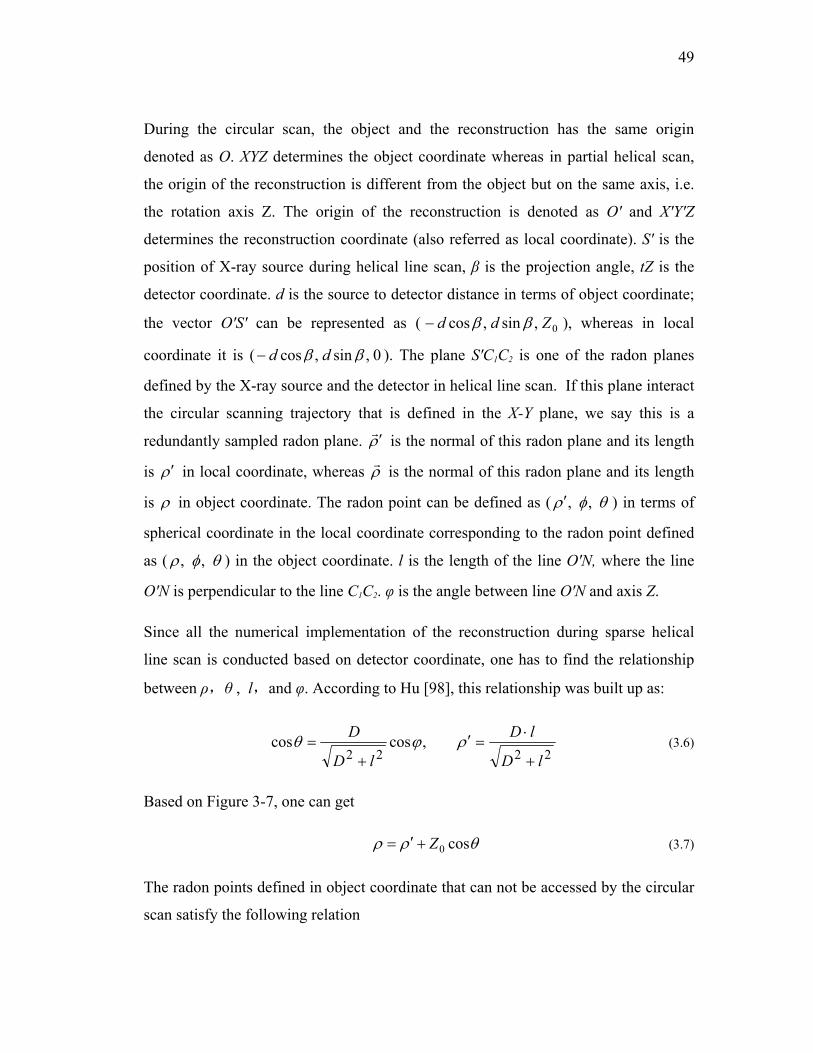
49
During the circular scan, the object and the reconstruction has the same origin
denoted as O. XYZ determines the object coordinate whereas in partial helical scan,
the origin of the reconstruction is different from the object but on the same axis, i.e.
the rotation axis Z. The origin of the reconstruction is denoted as O' and X'Y'Z
determines the reconstruction coordinate (also referred as local coordinate). S' is the
position of X-ray source during helical line scan, β is the projection angle, tZ is the
detector coordinate. d is the source to detector distance in terms of object coordinate;
the vector O'S' can be represented as ( 0,sin,cos Zdd ββ− ), whereas in local
coordinate it is ( 0,sin,cos ββ dd− ). The plane S'C1C2 is one of the radon planes
defined by the X-ray source and the detector in helical line scan. If this plane interact
the circular scanning trajectory that is defined in the X-Y plane, we say this is a
redundantly sampled radon plane. ρr′ is the normal of this radon plane and its length
is ρ′ in local coordinate, whereas ρr
is the normal of this radon plane and its length
is ρ in object coordinate. The radon point can be defined as ( θφρ ,,′ ) in terms of
spherical coordinate in the local coordinate corresponding to the radon point defined
as ( θφρ ,, ) in the object coordinate. l is the length of the line O'N, where the line
O'N is perpendicular to the line C1C2. φ is the angle between line O'N and axis Z.
Since all the numerical implementation of the reconstruction during sparse helical
line scan is conducted based on detector coordinate, one has to find the relationship
between ρ,θ , l,and φ. According to Hu [98], this relationship was built up as:
2222
,coscoslD
lD
lD
D
+
⋅=′
+= ρϕθ (3.6)
Based on Figure 3-7, one can get
θρρ cos0Z+′= (3.7)
The radon points defined in object coordinate that can not be accessed by the circular
scan satisfy the following relation
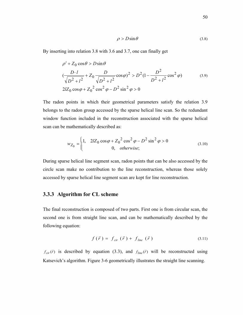
50
θρ sinD> (3.8)
By inserting into relation 3.8 with 3.6 and 3.7, one can finally get
0sincoscos2
)cos1()cos(
sincos
222200
222
222
22022
0
>−+
+−>
++
+
⋅
>+′
ϕϕϕ
ϕϕ
θθρ
DZlZ
lDDD
lD
DZlD
lD
DZ
(3.9)
The radon points in which their geometrical parameters satisfy the relation 3.9
belongs to the radon group accessed by the sparse helical line scan. So the redundant
window function included in the reconstruction associated with the sparse helical
scan can be mathematically described as:
⎪⎩
⎪⎨⎧ >−+=
;,00sincoscos2,1 2222
000 otherwise
DZlZwZϕϕϕ
(3.10)
During sparse helical line segment scan, radon points that can be also accessed by the
circle scan make no contribution to the line reconstruction, whereas those solely
accessed by sparse helical line segment scan are kept for line reconstruction.
3.3.3 Algorithm for CL scheme
The final reconstruction is composed of two parts. First one is from circular scan, the
second one is from straight line scan, and can be mathematically described by the
following equation:
)()()( rfrfrf linecirrrr
+= (3.11)
)(rf cirr is described by equation (3.3), and )(rf line
r will be reconstructed using
Katsevich’s algorithm. Figure 3-6 geometrically illustrates the straight line scanning.
51
Figure 3-6 Illustration of straight line scanning
The curve described by )(xz on the virtual detector is the projection of circle
trajectory seen from the current X-ray source. )(rf liner is mathematically described as:
dldrllyPlrly
rf line ∫ ∫ Θ∂∂
−−=
π
γγγ
π
2
02 sin
)),,(),(()(1
21)( rrr
rrr
(3.12)
The implementation of the )(rf liner can be referred to [102-103]. Please note that
under the current CBBCT geometry, the curve )(xz is described mathematically as:
⎥⎦⎤
⎢⎣⎡ −= 2)(12)(
dxHxz (3.13)
Apparently, this is a parabola with its vertex at )2,0( H , where z and x are the
vertical and horizontal coordinates on the detector, and H is the distance of the X-ray
source to the circular scanning plane. The filtering lines (on which the Hilbert
filtering is conducted) are determined by the intersection of the flat panel detector
52
with the planes tangent to the curve )(xz . On the detector, this line can be described
as bKxxz l +=)( , where2
Hb > . By inserting this line equation into (3.13), the
tangent filtering lines can be described as:
bxd
HHbxzl +−
±=22)( (3.14)
b is actually the intersection of those lines with the Z axis and can be used as an
index parameter. Note from (3.14) that there are two sets of filtering lines that can
provide the double coverage of the detector area above the curve )(xz . Hilbert
filtering on these two sets of lines should be carefully treated since Hilbert filtering is
sensitive to the filtering direction. In the current simulation, contributions from these
two sets of filtering lines are added.
3.4 Performance evaluation through computer
simulation
3.4.1 Description of the numerical breast phantom & scanning
parameters
Computer simulations were carried out on a numerical breast phantom that was
created for this study. This breast phantom is a half-ellipsoid with three half-axes of
8.8, 8.8 and 16 cm, specifically designed to address the artifacts resulting from the
single circular scan. The phantom is wrapped by simulated skin with a thickness of 2
mm. Within the simulated skin, the base material is a compound of adipose and
glandular tissues (e.g. 50% adipose and 50% glandular). There are three groups of
objects inside the breast phantom. Within first two groups are two sets of spheres: one
set of carcinoma spheres with diameters of 1, 2, 4, 6, and 8 mm, respectively and are

53
located at the positions where Z = 10, 70, 130 mm from the chest wall; and one set of
glandular spheres with diameters of 1, 2, 4, 6, and 8 mm, respectively and are located
at the same position as the group of carcinoma spheres. The third group is composed
of two low contrast disk-type objects specifically constructed to address the
geometrical deformation of the reconstructed objects around the nipple area and are
located at the position where Z = 148 mm from the chest wall. The disc length along
the X, Y and Z-axis is 10, 10 and 2.5 mm, respectively. The linear attenuation
coefficients with respect to skin, base material, carcinoma, glandular, and disk-type
object are 0.22, 0.19, 0.23, 0.24 and 0.21, respectively. The distance between the x-
ray source and the rotation center is 650 mm and the practical detector pixel size is
0.388 mm; the magnification factor is 1.43; the detector size is 660 by 660. The value
of the reconstructed images is converted to CT number by using the 0.25 as the linear
attenuation coefficient of water. Table 1 and 2 summarize scanning parameters
associated with two auxiliary scanning schemes.
Table 3-1 Partial helical line scanning parameters
Iso Distance 650 mm # of detector row 661
Magnification factor 1.43 # of Detector column 661
Detector pixel pitch 0.388 mm Starting position (Helical line scan)
Z = 49 mm
# of projections in circle 300 Ending position (Helical line scan)
Z = 121 mm
# of projections in helical line 32
(64)
Sampling interval along Z axis (Helical line scan)
Δl = 2.34 mm
Δl = 1.15 mm
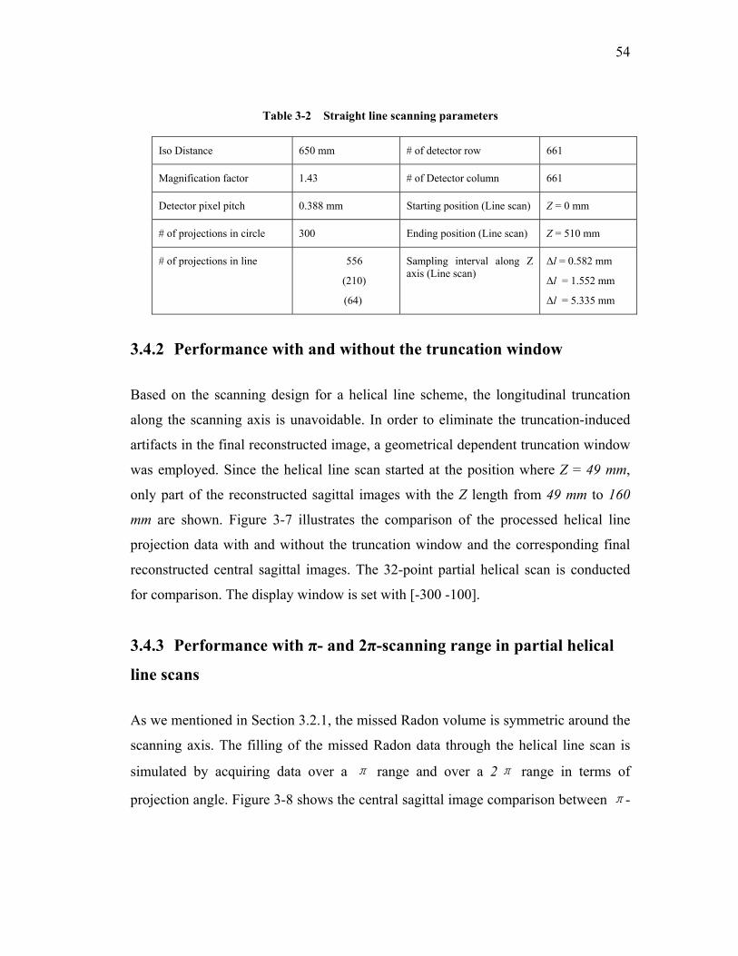
54
Table 3-2 Straight line scanning parameters
Iso Distance 650 mm # of detector row 661
Magnification factor 1.43 # of Detector column 661
Detector pixel pitch 0.388 mm Starting position (Line scan) Z = 0 mm
# of projections in circle 300 Ending position (Line scan) Z = 510 mm
# of projections in line 556
(210)
(64)
Sampling interval along Z axis (Line scan)
Δl = 0.582 mm
Δl = 1.552 mm
Δl = 5.335 mm
3.4.2 Performance with and without the truncation window
Based on the scanning design for a helical line scheme, the longitudinal truncation
along the scanning axis is unavoidable. In order to eliminate the truncation-induced
artifacts in the final reconstructed image, a geometrical dependent truncation window
was employed. Since the helical line scan started at the position where Z = 49 mm,
only part of the reconstructed sagittal images with the Z length from 49 mm to 160
mm are shown. Figure 3-7 illustrates the comparison of the processed helical line
projection data with and without the truncation window and the corresponding final
reconstructed central sagittal images. The 32-point partial helical scan is conducted
for comparison. The display window is set with [-300 -100].
3.4.3 Performance with π- and 2π-scanning range in partial helical
line scans
As we mentioned in Section 3.2.1, the missed Radon volume is symmetric around the
scanning axis. The filling of the missed Radon data through the helical line scan is
simulated by acquiring data over a π range and over a 2π range in terms of
projection angle. Figure 3-8 shows the central sagittal image comparison between π-
55
and 2π-scanning ranges within a partial helical scan of 32 shooting points. The
display window is [-300 -100].
3.4.4 Performance with different sampling intervals in partial
helical line scans
The simulation was conducted in several settings as discussed in Section 3.2.2.
Figure 3-9 illustrates the comparison of the central sagittal image from CHL scheme
with different sampling rate during helical line scan and phantom. The angular
scanning range is 2π within a partial helical scan. The objects at different layers
within the breast are simulated tumors with different sizes. The display window is [-
300 -100].
3.4.5 Performance with different sampling intervals in straight line
scan
The contribution from straight line scan was reconstructed using Katsevich’s
algorithm. Figure 3-10 shows the central sagittal image comparison between phantom
and CL scan scheme with different sampling interval along the line scanning
trajectory. The display window is [-300 -100].
3.4.6 Profile comparison between phantom, MFDK, CHL and CL
scanning schemes
Figure 3-11 shows the profile comparison in the central sagittal images from different
scanning schemes of MFDK, CHL, CL and the phantom.
56
3.5 The Experimental Breast Phantom Study
The CHL scanning scheme evaluation based on the breast phantom was conducted on
a prototype breast cone beam CT. It is a totally new customized CT system. The
system is made up of a slip ring featured horizontally rotating gantry, a
mammography x-ray tube, a Varian 40 by 30 cm flat panel detector and a patient
table. During the experiment, a D-cup breast phantom (21.5 x 17 x 10 cm) was used.
Based on the iso-distance of 650 mm, the cone angle spanned by this breast phantom
is 8.75 degrees. During the circular scan, the whole breast was projected onto the
detector and it took 10 seconds to acquire 300 projection images. Then the patient
table on which the breast phantom hung was lifted up 30 mm to simulate the partial
helical line scan by adopting a step shot mode in which 30 projection images were
acquired. A line increment and projection angle interval of 1.6 mm and 12 degrees
were used. The x-ray settings used were 49 kVp, 200mA and 8 ms pulse width.
Figure 3-14 illustrates the reconstructed cross and coronal images from circular and
CHL scans. All the images are shown with the display window of [-640 –500]. Line
profile comparisons are illustrated in Figure3-12(e) and (f) showing that the circle
plus helical line scan scheme can contribute to the correctness of the geometrical
deformation around the nipple area and improvement of the density drop along the
rotation axis inherited in a single FDK circular scan scheme. The projection image
Figure3-12(g) made during the partial helical line scan with the projection angle of 0
degrees is used to accentuate the geometrical correctness of the CHL scan scheme in
Figure3-12(d). A box of 100 by 100 pixels was inserted into the center of the images
in Fig 12(a) and (b) and noise level (standard deviation) was measured within the box.
The noise level from the circle FDK reconstruction is 6.03 whereas the noise level
from the CH scanning reconstruction is 5.89.
57
3.6 Discussion and conclusion
The new scanning scheme of CHL scan works better than a single circular scan in
terms of image uniformity and geometrical correctness based on the computer
simulations of a numerical breast phantom and a simulated breast phantom CBBCT
prototype study. As described in Section 3.2.2, the filling of the missed Radon data in
the volume by the partial helical scan through a 2π-scanning range resulted in a better
image reconstruction than through a π-scanning range since more streak artifacts are
shown in π-scanning range reconstruction. The object geometry-dependent truncation
window included in the equation (3.5) can efficiently eliminate the truncation artifacts
during the partial helical scan. Partial helical line scan with different sampling
interval showed that the number of X-ray shootings between 32 and 64 could provide
acceptable reconstructed images in terms of correction to the intensity drop along the
scanning axis and geometrical deformation around the nipple area based on the
scanning geometrical parameters and breast size. This is encouraging, since the
quality of reconstructed images could improve without too much additional radiation
exposure to the patient. Also note that the smaller the sampling interval (the larger the
number of projections) in helical line scan, the less the streak artifacts in the corrected
area. However, these streak artifacts are faintly visible. In practical situation, the
image quality should be balanced with the sampling interval in helical line scan. This
new scanning scheme is not intended to conduct an exact reconstruction.
Theoretically, when the missing volume in Radon domain is completely filled and at
least as densely sampled as those accessed by circle scan, the combined
reconstruction is exact. By sparsely sampling the missing volume through a proposed
scanning scheme, it suffices to correct the artifacts occurring in a single circular scan.
On the other hand, the new scanning scheme is easy to operate in practice without
much mechanical modification on the current CBBCT system.
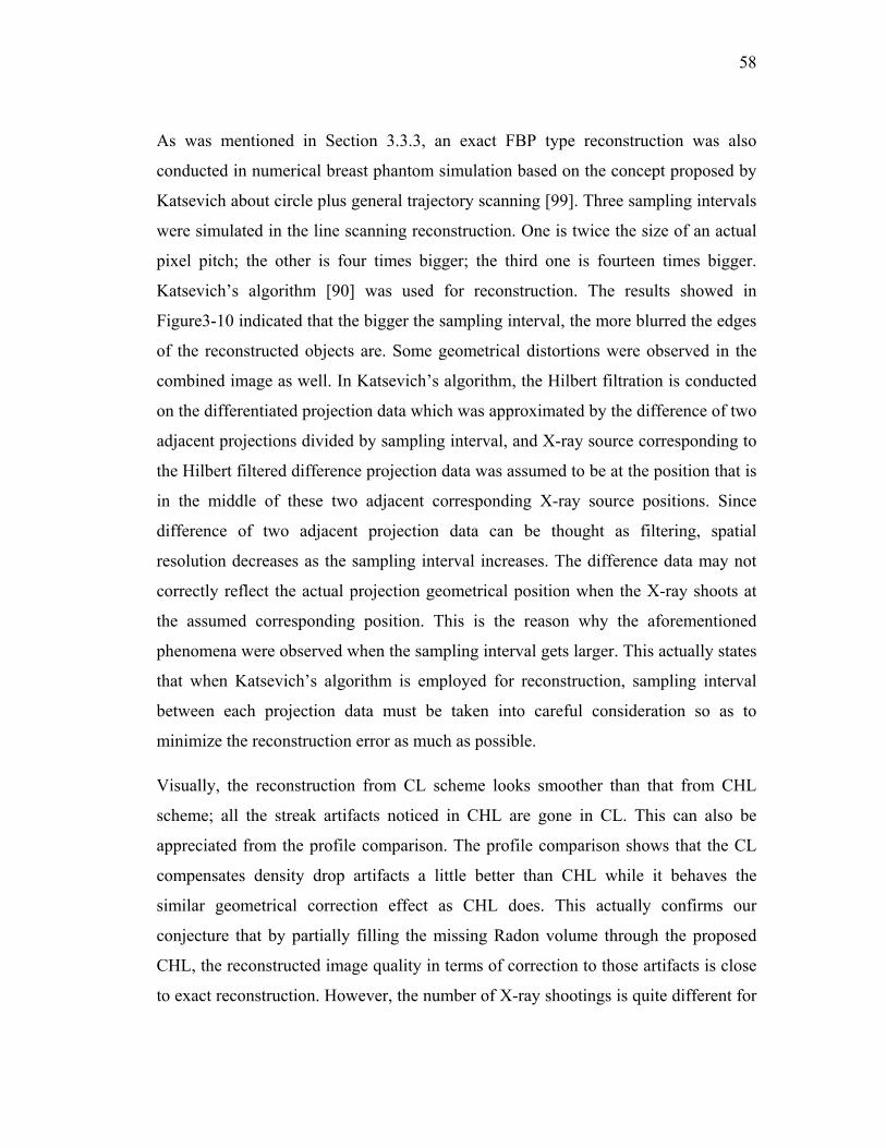
58
As was mentioned in Section 3.3.3, an exact FBP type reconstruction was also
conducted in numerical breast phantom simulation based on the concept proposed by
Katsevich about circle plus general trajectory scanning [99]. Three sampling intervals
were simulated in the line scanning reconstruction. One is twice the size of an actual
pixel pitch; the other is four times bigger; the third one is fourteen times bigger.
Katsevich’s algorithm [90] was used for reconstruction. The results showed in
Figure3-10 indicated that the bigger the sampling interval, the more blurred the edges
of the reconstructed objects are. Some geometrical distortions were observed in the
combined image as well. In Katsevich’s algorithm, the Hilbert filtration is conducted
on the differentiated projection data which was approximated by the difference of two
adjacent projections divided by sampling interval, and X-ray source corresponding to
the Hilbert filtered difference projection data was assumed to be at the position that is
in the middle of these two adjacent corresponding X-ray source positions. Since
difference of two adjacent projection data can be thought as filtering, spatial
resolution decreases as the sampling interval increases. The difference data may not
correctly reflect the actual projection geometrical position when the X-ray shoots at
the assumed corresponding position. This is the reason why the aforementioned
phenomena were observed when the sampling interval gets larger. This actually states
that when Katsevich’s algorithm is employed for reconstruction, sampling interval
between each projection data must be taken into careful consideration so as to
minimize the reconstruction error as much as possible.
Visually, the reconstruction from CL scheme looks smoother than that from CHL
scheme; all the streak artifacts noticed in CHL are gone in CL. This can also be
appreciated from the profile comparison. The profile comparison shows that the CL
compensates density drop artifacts a little better than CHL while it behaves the
similar geometrical correction effect as CHL does. This actually confirms our
conjecture that by partially filling the missing Radon volume through the proposed
CHL, the reconstructed image quality in terms of correction to those artifacts is close
to exact reconstruction. However, the number of X-ray shootings is quite different for
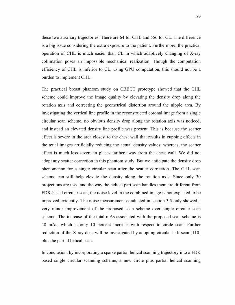
59
these two auxiliary trajectories. There are 64 for CHL and 556 for CL. The difference
is a big issue considering the extra exposure to the patient. Furthermore, the practical
operation of CHL is much easier than CL in which adaptively changing of X-ray
collimation poses an impossible mechanical realization. Though the computation
efficiency of CHL is inferior to CL, using GPU computation, this should not be a
burden to implement CHL.
The practical breast phantom study on CBBCT prototype showed that the CHL
scheme could improve the image quality by elevating the density drop along the
rotation axis and correcting the geometrical distortion around the nipple area. By
investigating the vertical line profile in the reconstructed coronal image from a single
circular scan scheme, no obvious density drop along the rotation axis was noticed,
and instead an elevated density line profile was present. This is because the scatter
effect is severe in the area closest to the chest wall that results in cupping effects in
the axial images artificially reducing the actual density values; whereas, the scatter
effect is much less severe in places farther away from the chest wall. We did not
adopt any scatter correction in this phantom study. But we anticipate the density drop
phenomenon for a single circular scan after the scatter correction. The CHL scan
scheme can still help elevate the density along the rotation axis. Since only 30
projections are used and the way the helical part scan handles them are different from
FDK-based circular scan, the noise level in the combined image is not expected to be
improved evidently. The noise measurement conducted in section 3.5 only showed a
very minor improvement of the proposed scan scheme over single circular scan
scheme. The increase of the total mAs associated with the proposed scan scheme is
48 mAs, which is only 10 percent increase with respect to circle scan. Further
reduction of the X-ray dose will be investigated by adopting circular half scan [110]
plus the partial helical scan.
In conclusion, by incorporating a sparse partial helical scanning trajectory into a FDK
based single circular scanning scheme, a new circle plus partial helical scanning

60
scheme was proposed to compensate for the artifacts inherited by a single circular
scan. The numerical simulation and simulated breast phantom study have
demonstrated its feasibility.
(a)
(b) (c)
(d)
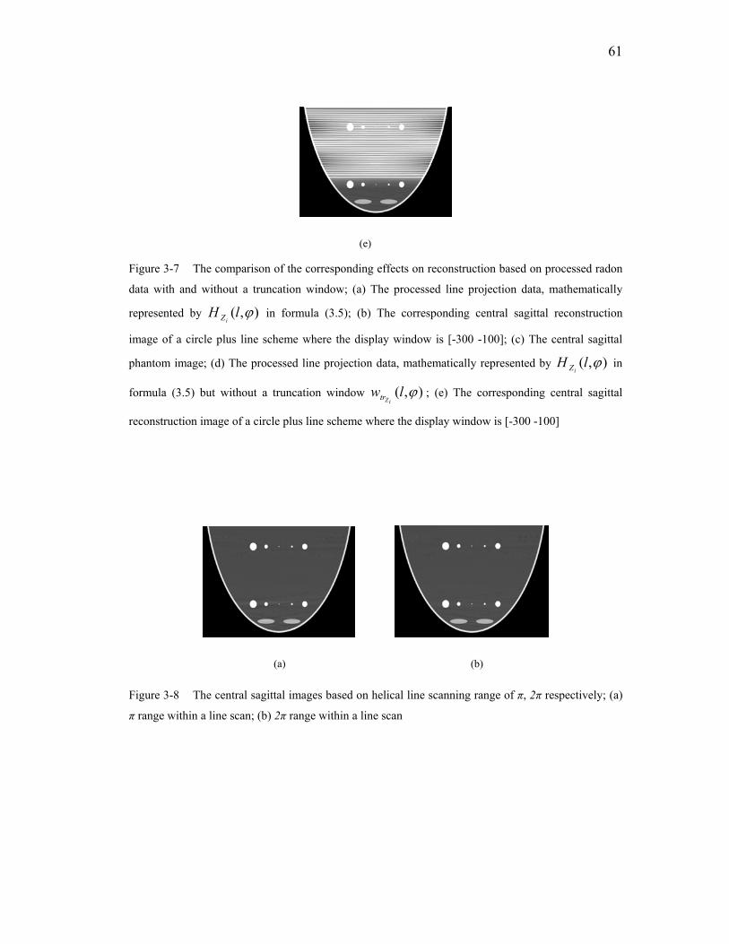
61
(e)
Figure 3-7 The comparison of the corresponding effects on reconstruction based on processed radon
data with and without a truncation window; (a) The processed line projection data, mathematically
represented by ),( ϕlHiZ in formula (3.5); (b) The corresponding central sagittal reconstruction
image of a circle plus line scheme where the display window is [-300 -100]; (c) The central sagittal
phantom image; (d) The processed line projection data, mathematically represented by ),( ϕlHiZ in
formula (3.5) but without a truncation window ),( ϕlwiZtr ; (e) The corresponding central sagittal
reconstruction image of a circle plus line scheme where the display window is [-300 -100]
(a) (b)
Figure 3-8 The central sagittal images based on helical line scanning range of π, 2π respectively; (a)
π range within a line scan; (b) 2π range within a line scan
62
(a) (b) (c)
(d) (e) (f)
(g) (h) (i)
(j)
Figure 3-9 Central sagittal image comparison between MFDK, phantom and partial helical line term
with different sampling interval; (a) FDK; (b) Hui term; (c) MFDK; (d) MFDK; (e) HL recon (32
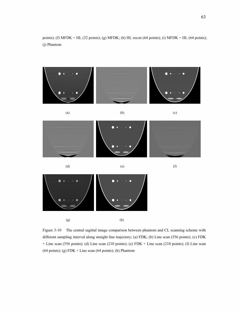
63
points); (f) MFDK + HL (32 points); (g) MFDK; (h) HL recon (64 points); (i) MFDK + HL (64 points);
(j) Phantom
(a) (b) (c)
(d) (e) (f)
(g) (h)
Figure 3-10 The central sagittal image comparison between phantom and CL scanning scheme with
different sampling interval along straight line trajectory; (a) FDK; (b) Line scan (556 points); (c) FDK
+ Line scan (556 points); (d) Line scan (210 points); (e) FDK + Line scan (210 points); (f) Line scan
(64 points); (g) FDK + Line scan (64 points); (h) Phantom
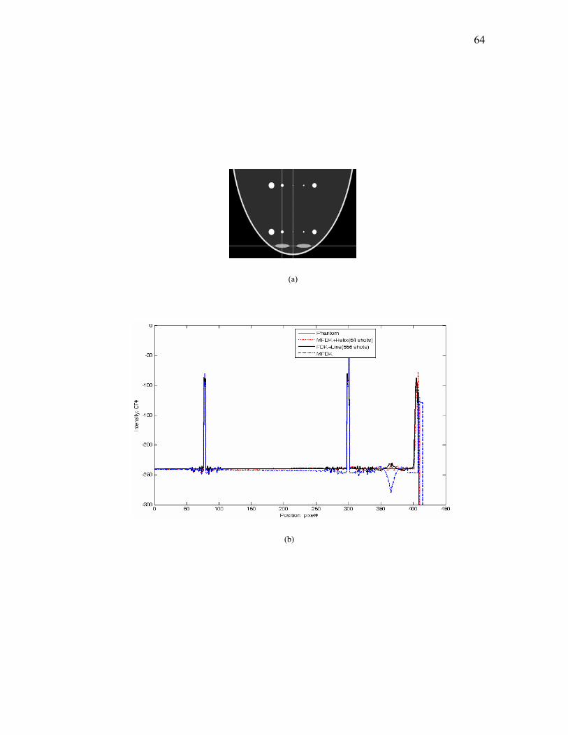
64
(a)
(b)
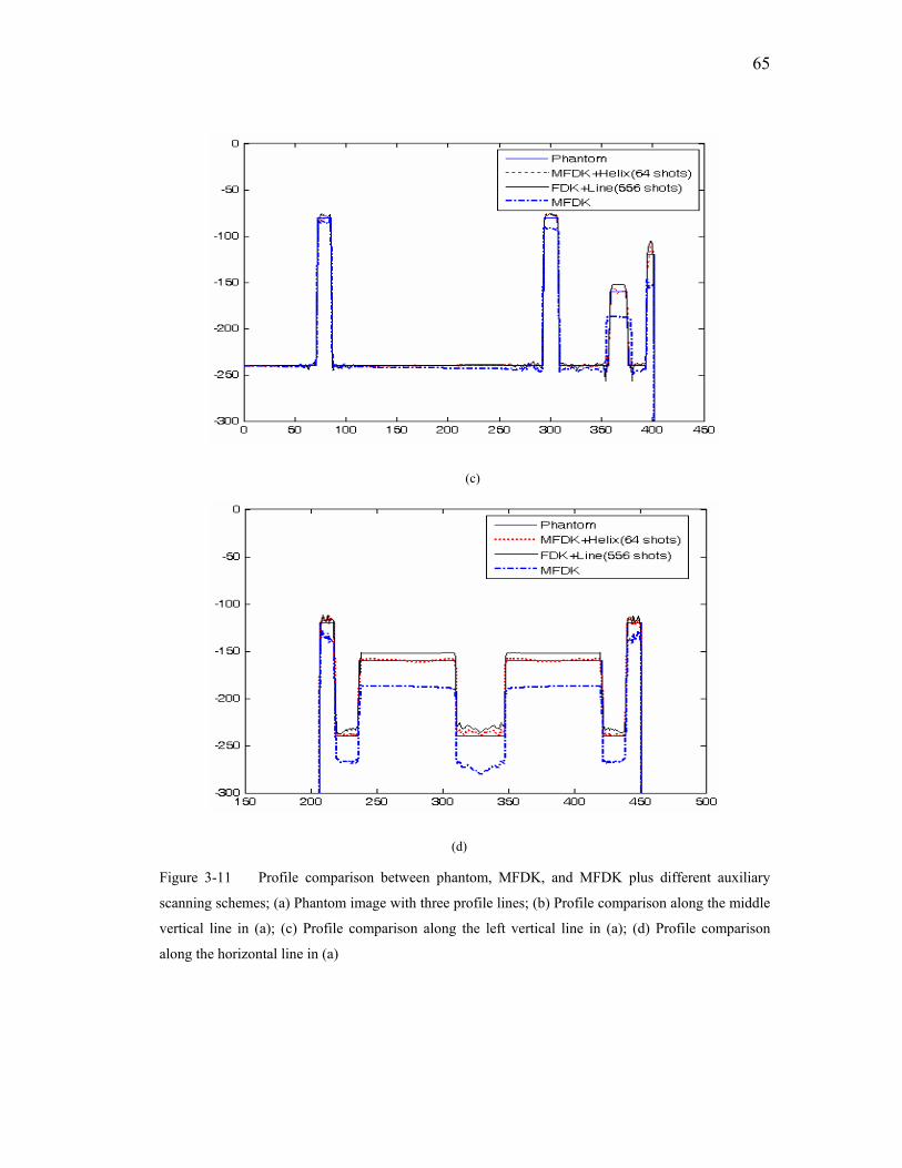
65
(c)
(d)
Figure 3-11 Profile comparison between phantom, MFDK, and MFDK plus different auxiliary
scanning schemes; (a) Phantom image with three profile lines; (b) Profile comparison along the middle
vertical line in (a); (c) Profile comparison along the left vertical line in (a); (d) Profile comparison
along the horizontal line in (a)
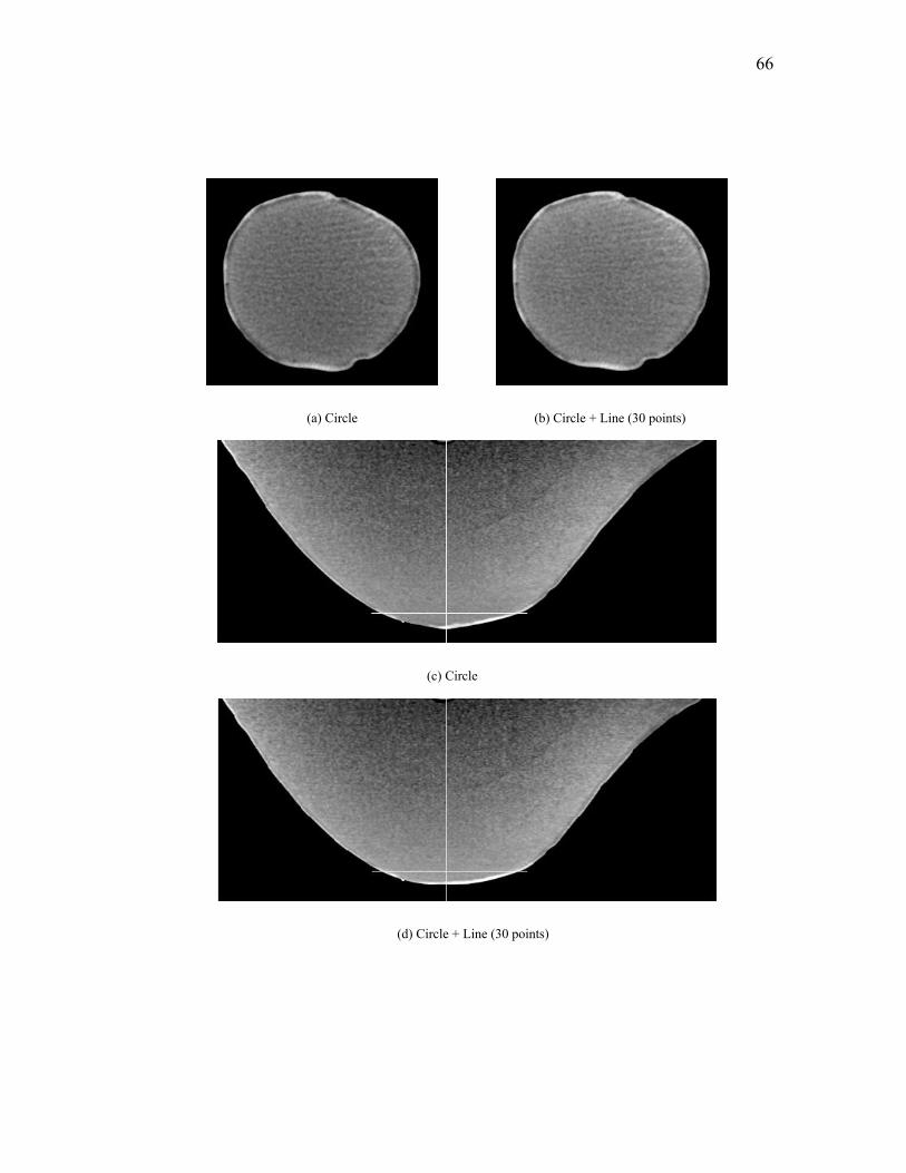
66
(a) Circle (b) Circle + Line (30 points)
(c) Circle
(d) Circle + Line (30 points)
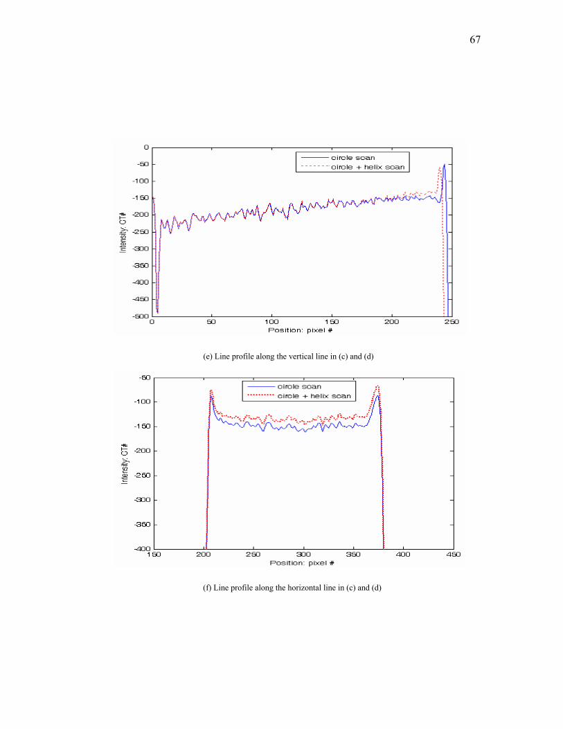
67
(e) Line profile along the vertical line in (c) and (d)
(f) Line profile along the horizontal line in (c) and (d)
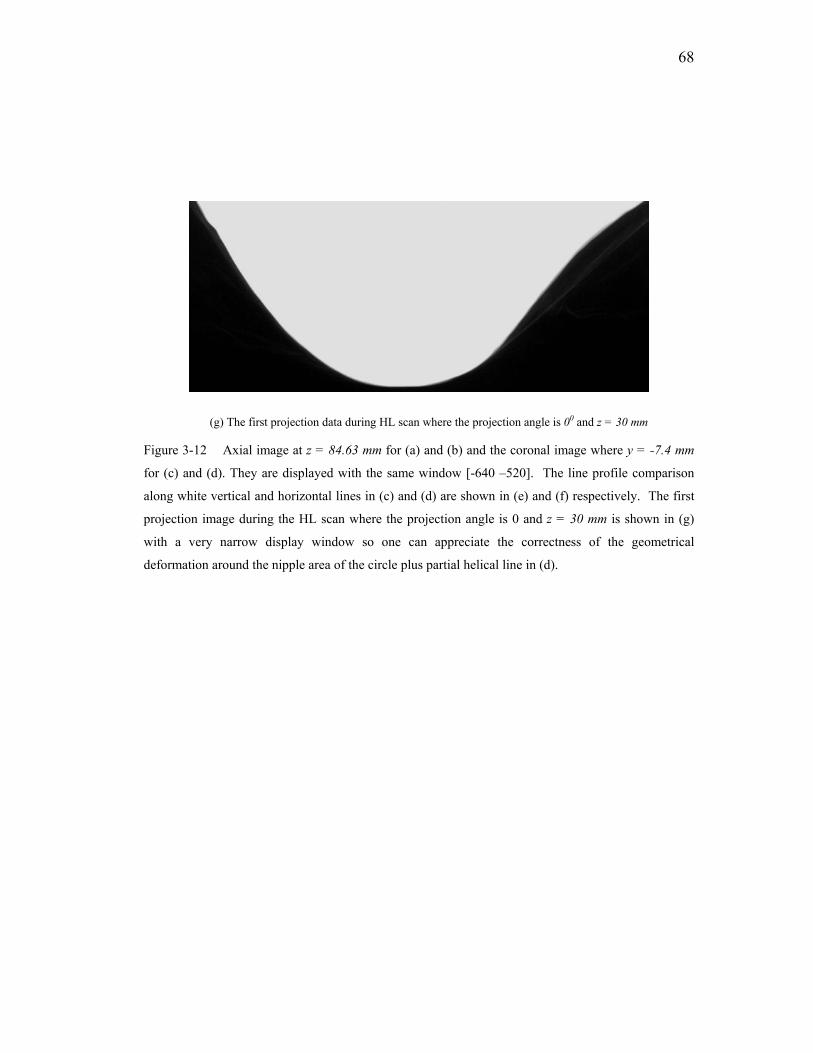
68
(g) The first projection data during HL scan where the projection angle is 00 and z = 30 mm
Figure 3-12 Axial image at z = 84.63 mm for (a) and (b) and the coronal image where y = -7.4 mm
for (c) and (d). They are displayed with the same window [-640 –520]. The line profile comparison
along white vertical and horizontal lines in (c) and (d) are shown in (e) and (f) respectively. The first
projection image during the HL scan where the projection angle is 0 and z = 30 mm is shown in (g)
with a very narrow display window so one can appreciate the correctness of the geometrical
deformation around the nipple area of the circle plus partial helical line in (d).
69
Chapter 4 Circular Half-Scan Cone Beam
Reconstruction
4.1 Traditional circular cone beam half-scan scheme
Half-scan scheme on cone beam CT has been a hot topic in recent years due to the
improvement in the temporal resolution [104, 105] and possible reduction of the x-ray
dose deposited in the patient. There are several kinds of cone beam half-scan schemes
available currently. One is FDK-type based [60, 106]. Another one is the cone beam
filtered-backprojection (CBFBP) [107]. The other one is Grangeat-type based [108].
They use either planar scanning trajectory (circular or non-circular) or non-planar
scanning trajectory to conduct the half-scan scheme. Grangeat-type half-scan (GHS)
maps the space projection data into the radon domain and weights them in the radon
domain, after adding missing data in the shadow zone of the radon domain through
linear interpolation/extrapolation, get the reconstructed image by Grangeat formula
[77]. Currently, FDK-type half-scan schemes have two types. One (FDK-HSFW)
applies the Parker’s [109] or other weighting coefficients based on the scanning plane
fan beam geometry to the cone beam projection data. In other words, the same
weighting coefficient is applied to all of the detector rows. The other (FDK-HSCW),
which was heuristically developed by us applied cone beam geometry dependent
weighting coefficients to the projection data [110]. FDK-HSCW outperforms FDK-
HSFW in terms of the correction of the attenuation coefficient drop along the
70
scanning axis when cone angle becomes large. The CBFBP algorithm manipulates the
redundant projection data in the space domain and then does the half-scan
reconstruction getting almost the same performance as FDK-HSFW does. The
Grangeat-type half-scan scheme outperforms the FDK-type half-scan scheme in terms
of the less attenuation coefficient drop along the scanning axis and better geometrical
correction when the shadow zone is filled with the linear interpolated data in the
radon domain. But the spatial resolution of the reconstructed images from GHS is
inferior to the ones from FDK-FS, FDK-HSFW, and FDK-HSCW. This is because
the data interpolation is less involved in FDK than in GHS [111].
Though FDK-HSCW works better than FDK-FS & FDK-HSFW in terms of
correction of the attenuation coefficient drop, it still showed the obvious attenuation
coefficient drop artifacts in the position that is farther away from Z = 0 (cone angle
becomes large, and Z is the rotation axis). This circular FDK inherited attenuation
coefficient drop property is undesirable in clinic practice.
In order to further improve FDK-HSCW by making full use of the information that
the half-circular scanning provides, we proposed a modified FDK half scan scheme
(MFDK-HS) which is composed of FDK-HSCW and a new supplementary term, a
FBP implementation developed by Hu Hui [97] to conduct the reconstruction task.
4.1.1 Traditional circular FDK cone beam half-scan algorithm
As we all know, the FDK algorithm [51] is the extension of the fan beam algorithm
by summing up the contribution to the object from all the tilted fan beams. The
reconstruction is based on filtering and back projecting a single fan beam within the
cone. Based on the cone-beam geometry in figure 4-1, the formula of the FDK can be
described as:
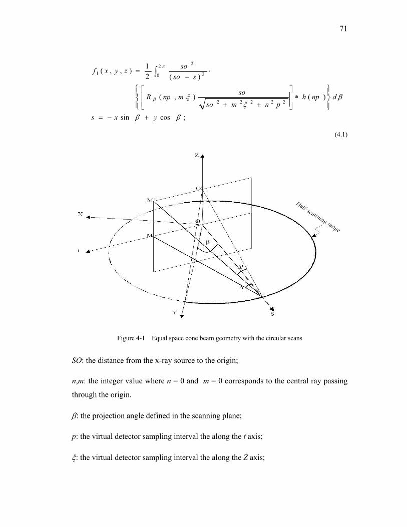
71
;cossin
)(),(
)(21),,(
22222
2
0 2
2
1
ββ
βξ
ξβ
π
yxs
dnphpnmso
somnpR
ssosozyxf
+−=
⎪⎭
⎪⎬⎫
⎪⎩
⎪⎨⎧
∗⎥⎥⎦
⎤
⎢⎢⎣
⎡
++
⋅−
= ∫
(4.1)
Figure 4-1 Equal space cone beam geometry with the circular scans
SO: the distance from the x-ray source to the origin;
n,m: the integer value where n = 0 and m = 0 corresponds to the central ray passing
through the origin.
β: the projection angle defined in the scanning plane;
p: the virtual detector sampling interval the along the t axis;
ξ: the virtual detector sampling interval the along the Z axis;
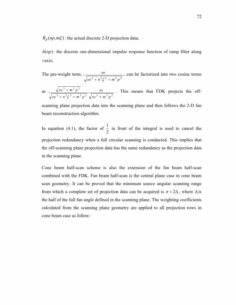
72
),( ξβ mnpR : the actual discrete 2-D projection data;
:)(nph the discrete one-dimensional impulse response function of ramp filter along
t axis;
The pre-weight term, 22222 pmnso
so
++ ξ, can be factorized into two cosine terms
as 22222222
222
pmso
so
pmnso
pmso
+++
+
ξ. This means that FDK projects the off-
scanning plane projection data into the scanning plane and then follows the 2-D fan
beam reconstruction algorithm.
In equation (4.1), the factor of 21 in front of the integral is used to cancel the
projection redundancy when a full circular scanning is conducted. This implies that
the off-scanning plane projection data has the same redundancy as the projection data
in the scanning plane.
Cone beam half-scan scheme is also the extension of the fan beam half-scan
combined with the FDK. Fan beam half-scan is the central plane case in cone beam
scan geometry. It can be proved that the minimum source angular scanning range
from which a complete set of projection data can be acquired is Δ+ 2π , where Δ is
the half of the full fan angle defined in the scanning plane. The weighting coefficients
calculated from the scanning plane geometry are applied to all projection rows in
cone beam case as follow:
73
{
;cossin
)(]
),(),([)(
),,(
22222
2
0 2
2
1
ββ
βξ
βξπ
β
yxs
dnphpnmso
so
npwmnpRsso
sozyxf
+−=
⎪⎭
⎪⎬⎫
∗++
×
⋅⋅−
= ∫ ∫Δ+ ∞
∞−
(4.2)
This is the FDK fan beam half-scan weighting scheme (FDK-HSFW). The off-
scanning plane projection data are still treated as they have the same redundancy.
),( npβω is the weighting coefficients calculated based on the scanning plane
geometry, and can be represented by Parker’s weighting function or any other
weighting function as long as it can make a smooth transition of the projection data
between the doubly and singly sampled regions to avoid discontinuities at the borders
of these regions. Undoubtedly, FDK-HSFW holds all the properties that FDK full
scan scheme does.
4.2 Modified circular FDK cone beam half-scan
algorithm
For cone beam projection data off the scanning plane, it is impossible to obtain
doubly sampled projections for a single orbit acquisition even if projections are
sampled over 360° [59]. In other words, the projection redundancy becomes less and
less when projection rows get further away from the scanning plane. If the FDK
algorithm was directly applied to half-scan projection data that is not weighted, the
reconstructed images would unavoidably have artifacts. One way to handle the
weighting on the less redundancy projection row data away from scanning plane is
proposed in the following section.
74
4.2.1 Heuristic circular cone beam half-scan weighting scheme
In a circular fan-beam half-scan, there are two redundant regions in the scanning
plane in terms of the projection angle β. Figure 4-2 shows that the projecting ray data
acquired in region I will have a conjugate ray data in region II. In these two regions,
Figure 4-2 Illustration of redundant regions in terms of projection angle in circular fan-beam half-
scan
the projection ray data is wholly or partly redundant. If half of the full fan angle is Δ
degrees, the half scan range in terms of projection angle defined in the scanning plane
is from 00 to 1800 + 2Δ. The first and second redundant region is from 00 to 4Δ and
from 1800 - 2Δ to 1800 + 2Δ respectively. In the traditional FDK cone-beam half scan
scheme, all the row projection data are weighted by the same set of coefficients
defined in the scanning plane because the row projection data away from the scanning
plane are expected to have the same redundancy as those in the scanning plane.
The proposal of the circular cone-beam half scan weighting scheme is based on the
idea that the weighting coefficients should be different for projection data in different
rows. For the row projection data furthest away from the scanning plane, it should be
weighted less. As of this date, we have not seen any literature discussing this issue.
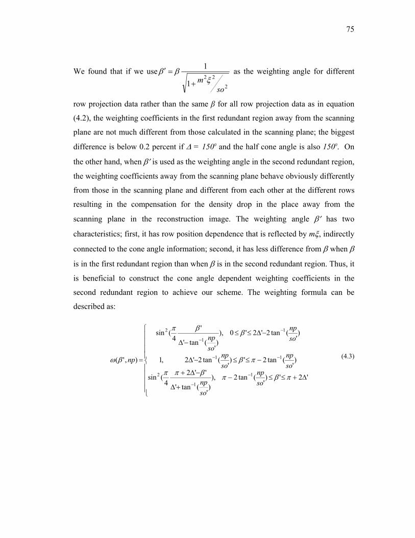
75
We found that if we use
2
221
1
som ξ
ββ+
=′ as the weighting angle for different
row projection data rather than the same β for all row projection data as in equation
(4.2), the weighting coefficients in the first redundant region away from the scanning
plane are not much different from those calculated in the scanning plane; the biggest
difference is below 0.2 percent if Δ = 1500 and the half cone angle is also 1500. On
the other hand, when β′ is used as the weighting angle in the second redundant region,
the weighting coefficients away from the scanning plane behave obviously differently
from those in the scanning plane and different from each other at the different rows
resulting in the compensation for the density drop in the place away from the
scanning plane in the reconstruction image. The weighting angle β′ has two
characteristics; first, it has row position dependence that is reflected by mξ, indirectly
connected to the cone angle information; second, it has less difference from β when β
is in the first redundant region than when β is in the second redundant region. Thus, it
is beneficial to construct the cone angle dependent weighting coefficients in the
second redundant region to achieve our scheme. The weighting formula can be
described as:
⎪⎪⎪⎪
⎩
⎪⎪⎪⎪
⎨
⎧
Δ+≤≤−+Δ
−Δ+
−≤≤−Δ
−Δ≤≤−Δ
=
−
−
−−
−
−
'2')'
(tan2),)'
(tan'
''24
(sin
)'
(tan2')'
(tan2'2,1
)'
(tan2'2'0),)'
(tan'
'4
(sin
),'(
1
1
2
11
1
1
2
πβπβππ
πβ
ββπ
βω
sonp
sonp
sonp
sonp
sonp
sonp
np (4.3)
76
);(tan'
'
1
1'
1
222
2
22
osMO
msoso
som
where
′=Δ
+=
+⋅=
−
ξ
ξββ
β ′ is the cone-weighting angle which was described previously. β ′ is dependent on
the position of the row projection data in the Z direction (rotation axis). Δ′ is half of
the titled fan angle that is adopted from Gullberg [59]. Notice that when m is zero,
this weighting function is actually the Parker’s weighting function for fan-beam.
By incorporating the cone-beam weighting function with the FDK, the FDK-HSCW
is obtained as follows:
;cossin
)}(]),(),'({[)(
),,(2
0 222222
2
1
ββ
βξ
ξβωπ
β
yxs
dnphpnmso
somnpRnpsso
sozyxf
+−=
∗++
⋅⋅⋅−
= ∫Δ+
(4.4)
Please note that the projection data must be weighted prior to being filtered. Since
FDK-HSFW is the commonly acknowledged scheme for half-scan reconstruction, the
requirement for FDK-HSCW is that it should produce no more artifacts than FDK-
HSFW.
4.2.2 Supplementary FBP term in circular cone beam half-scan
reconstruction
According to the derivation of the Grangeat’s algorithm, the relationship between
radon plane and the cone beam projections can be expressed as shown in Figure 4-3.
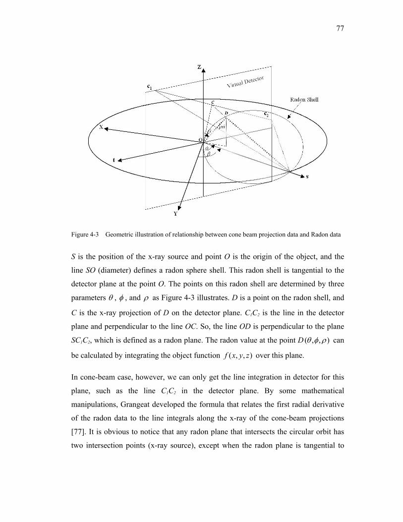
77
Figure 4-3 Geometric illustration of relationship between cone beam projection data and Radon data
S is the position of the x-ray source and point O is the origin of the object, and the
line SO (diameter) defines a radon sphere shell. This radon shell is tangential to the
detector plane at the point O. The points on this radon shell are determined by three
parameters θ , φ , and ρ as Figure 4-3 illustrates. D is a point on the radon shell, and
C is the x-ray projection of D on the detector plane. C1C2 is the line in the detector
plane and perpendicular to the line OC. So, the line OD is perpendicular to the plane
SC1C2, which is defined as a radon plane. The radon value at the point D ),,( ρφθ can
be calculated by integrating the object function ),,( zyxf over this plane.
In cone-beam case, however, we can only get the line integration in detector for this
plane, such as the line C1C2 in the detector plane. By some mathematical
manipulations, Grangeat developed the formula that relates the first radial derivative
of the radon data to the line integrals along the x-ray of the cone-beam projections
[77]. It is obvious to notice that any radon plane that intersects the circular orbit has
two intersection points (x-ray source), except when the radon plane is tangential to
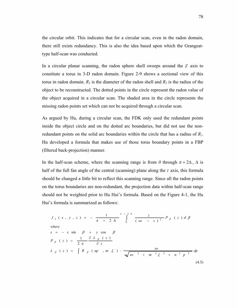
78
the circular orbit. This indicates that for a circular scan, even in the radon domain,
there still exists redundancy. This is also the idea based upon which the Grangeat-
type half-scan was conducted.
In a circular planar scanning, the radon sphere shell sweeps around the Z axis to
constitute a torus in 3-D radon domain. Figure 2-9 shows a sectional view of this
torus in radon domain. R1 is the diameter of the radon shell and R2 is the radius of the
object to be reconstructed. The dotted points in the circle represent the radon value of
the object acquired in a circular scan. The shaded area in the circle represents the
missing radon points set which can not be acquired through a circular scan.
As argued by Hu, during a circular scan, the FDK only used the redundant points
inside the object circle and on the dotted arc boundaries, but did not use the non-
redundant points on the solid arc boundaries within the circle that has a radius of R2.
Hu developed a formula that makes use of those torus boundary points in a FBP
(filtered back-projection) manner.
In the half-scan scheme, where the scanning range is from 0 through Δ+ 2π , Δ is
half of the full fan angle of the central (scanning) plane along the t axis, this formula
should be changed a little bit to reflect this scanning range. Since all the radon points
on the torus boundaries are non-redundant, the projection data within half-scan range
should not be weighted prior to Hu Hui’s formula. Based on the Figure 4-1, the Hu
Hui’s formula is summarized as follows:
∫
∫
++⋅=
∂
∂=
+−=
−Δ+−=
Δ+
dppnmso
somnpRz
zz
zP
yxswhere
dzPsso
zzyxf
22222
2
022
),()(
)(2
1)(
cossin
)()(2
1),,(
ξξλ
λπ
ββ
βπ
ββ
ββ
π
β
(4.5)
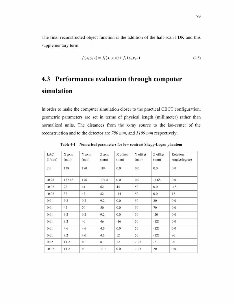
79
The final reconstructed object function is the addition of the half-scan FDK and this
supplementary term.
),,(),,(),,( 21 zyxfzyxfzyxf += (4.6)
4.3 Performance evaluation through computer
simulation
In order to make the computer simulation closer to the practical CBCT configuration,
geometric parameters are set in terms of physical length (millimeter) rather than
normalized units. The distances from the x-ray source to the iso-center of the
reconstruction and to the detector are 780 mm, and 1109 mm respectively.
Table 4-1 Numerical parameters for low contrast Shepp-Logan phantom
LAC (1/mm)
X axis (mm)
Y axis (mm)
Z axis (mm)
X offset (mm)
Y offset (mm)
Z offset (mm)
Rotation Angle(degree)
2.0 138 180 184 0.0 0.0 0.0 0.0
-0.98 132.48 176 174.8 0.0 0.0 -3.68 0.0
-0.02 22 44 62 44 50 0.0 -18
-0.02 32 42 82 -44 50 0.0 18
0.01 9.2 9.2 9.2 0.0 50 20 0.0
0.01 42 70 50 0.0 50 70 0.0
0.01 9.2 9.2 9.2 0.0 50 -20 0.0
0.01 9.2 40 46 -16 50 -121 0.0
0.01 4.6 4.6 4.6 0.0 50 -121 0.0
0.01 9.2 4.0 4.6 12 50 -121 90
0.02 11.2 40 8 12 -125 -21 90
-0.02 11.2 40 11.2 0.0 -125 20 0.0
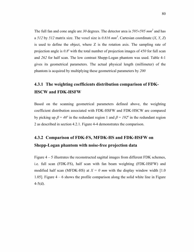
80
The full fan and cone angle are 30 degrees. The detector area is 595×595 mm2 and has
a 512 by 512 matrix size. The voxel size is 0.816 mm3. Cartesian coordinate (X, Y, Z)
is used to define the object, where Z is the rotation axis. The sampling rate of
projection angle is 0.80 with the total number of projection images of 450 for full scan
and 262 for half scan. The low contrast Shepp-Logan phantom was used. Table 4-1
gives its geometrical parameters. The actual physical length (millimeter) of the
phantom is acquired by multiplying these geometrical parameters by 200
4.3.1 The weighting coefficients distribution comparison of FDK-
HSCW and FDK-HSFW
Based on the scanning geometrical parameters defined above, the weighting
coefficient distribution associated with FDK-HSFW and FDK-HSCW are compared
by picking up β = 460 in the redundant region 1 and β = 1920 in the redundant region
2 as described in section 4.2.1. Figure 4-4 demonstrates the comparison.
4.3.2 Comparison of FDK-FS, MFDK-HS and FDK-HSFW on
Shepp-Logan phantom with noise-free projection data
Figure 4 – 5 illustrates the reconstructed sagittal images from different FDK schemes,
i.e. full scan (FDK-FS), half scan with fan beam weighting (FDK-HSFW) and
modified half scan (MFDK-HS) at X = 0 mm with the display window width [1.0
1.05]. Figure 4 – 6 shows the profile comparison along the solid white line in Figure
4-5(d).
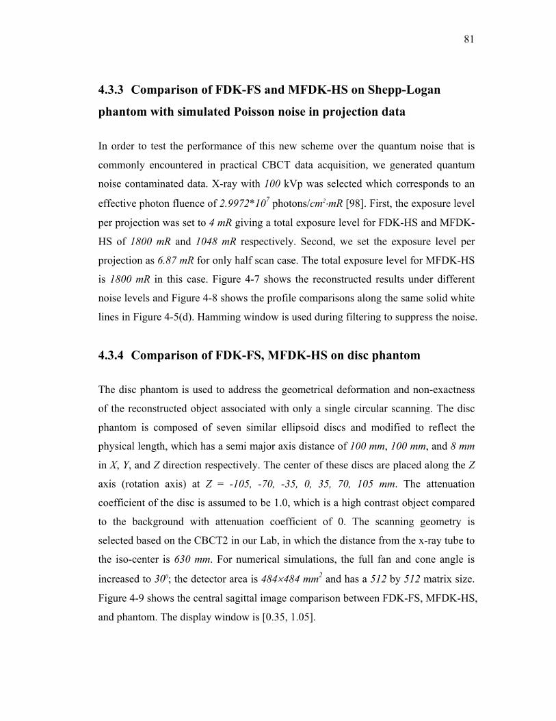
81
4.3.3 Comparison of FDK-FS and MFDK-HS on Shepp-Logan
phantom with simulated Poisson noise in projection data
In order to test the performance of this new scheme over the quantum noise that is
commonly encountered in practical CBCT data acquisition, we generated quantum
noise contaminated data. X-ray with 100 kVp was selected which corresponds to an
effective photon fluence of 2.9972*107 photons/cm2⋅mR [98]. First, the exposure level
per projection was set to 4 mR giving a total exposure level for FDK-HS and MFDK-
HS of 1800 mR and 1048 mR respectively. Second, we set the exposure level per
projection as 6.87 mR for only half scan case. The total exposure level for MFDK-HS
is 1800 mR in this case. Figure 4-7 shows the reconstructed results under different
noise levels and Figure 4-8 shows the profile comparisons along the same solid white
lines in Figure 4-5(d). Hamming window is used during filtering to suppress the noise.
4.3.4 Comparison of FDK-FS, MFDK-HS on disc phantom
The disc phantom is used to address the geometrical deformation and non-exactness
of the reconstructed object associated with only a single circular scanning. The disc
phantom is composed of seven similar ellipsoid discs and modified to reflect the
physical length, which has a semi major axis distance of 100 mm, 100 mm, and 8 mm
in X, Y, and Z direction respectively. The center of these discs are placed along the Z
axis (rotation axis) at Z = -105, -70, -35, 0, 35, 70, 105 mm. The attenuation
coefficient of the disc is assumed to be 1.0, which is a high contrast object compared
to the background with attenuation coefficient of 0. The scanning geometry is
selected based on the CBCT2 in our Lab, in which the distance from the x-ray tube to
the iso-center is 630 mm. For numerical simulations, the full fan and cone angle is
increased to 300; the detector area is 484×484 mm2 and has a 512 by 512 matrix size.
Figure 4-9 shows the central sagittal image comparison between FDK-FS, MFDK-HS,
and phantom. The display window is [0.35, 1.05].
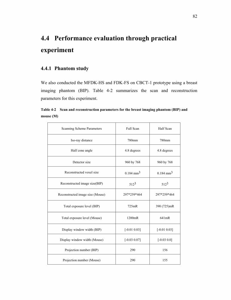
82
4.4 Performance evaluation through practical
experiment
4.4.1 Phantom study
We also conducted the MFDK-HS and FDK-FS on CBCT-1 prototype using a breast
imaging phantom (BIP). Table 4-2 summarizes the scan and reconstruction
parameters for this experiment.
Table 4-2 Scan and reconstruction parameters for the breast imaging phantom (BIP) and
mouse (M)
Scanning Scheme Parameters Full Scan Half Scan
Iso-ray distance 780mm 780mm
Half cone angle 4.8 degrees 4.8 degrees
Detector size 960 by 768 960 by 768
Reconstructed voxel size 0.184 mm3 0.184 mm3
Reconstructed image size(BIP) 5123 5123
Reconstructed image size (Mouse) 297*259*464 297*259*464
Total exposure level (BIP) 725mR 390 (725)mR
Total exposure level (Mouse) 1200mR 641mR
Display window width (BIP) [-0.01 0.03] [-0.01 0.03]
Display window width (Mouse) [-0.03 0.07] [-0.03 0.0]
Projection number (BIP) 290 156
Projection number (Mouse) 290 155
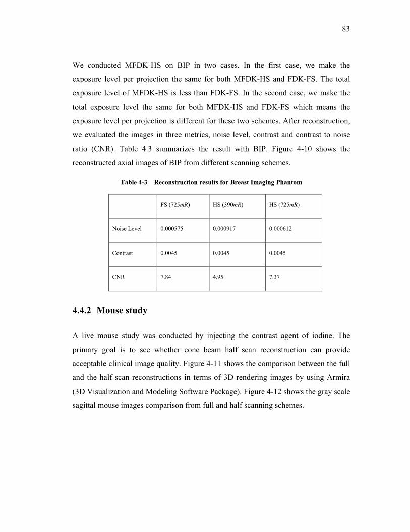
83
We conducted MFDK-HS on BIP in two cases. In the first case, we make the
exposure level per projection the same for both MFDK-HS and FDK-FS. The total
exposure level of MFDK-HS is less than FDK-FS. In the second case, we make the
total exposure level the same for both MFDK-HS and FDK-FS which means the
exposure level per projection is different for these two schemes. After reconstruction,
we evaluated the images in three metrics, noise level, contrast and contrast to noise
ratio (CNR). Table 4.3 summarizes the result with BIP. Figure 4-10 shows the
reconstructed axial images of BIP from different scanning schemes.
Table 4-3 Reconstruction results for Breast Imaging Phantom
FS (725mR) HS (390mR) HS (725mR)
Noise Level 0.000575 0.000917 0.000612
Contrast 0.0045 0.0045 0.0045
CNR 7.84 4.95 7.37
4.4.2 Mouse study
A live mouse study was conducted by injecting the contrast agent of iodine. The
primary goal is to see whether cone beam half scan reconstruction can provide
acceptable clinical image quality. Figure 4-11 shows the comparison between the full
and the half scan reconstructions in terms of 3D rendering images by using Armira
(3D Visualization and Modeling Software Package). Figure 4-12 shows the gray scale
sagittal mouse images comparison from full and half scanning schemes.
84
4.5 Discussion and conclusion
A new modified half-scan scheme (MFDK-HS) has been developed by adding a
supplementary term in the proposed FDK cone beam half scan (FDK-HSCW) scheme.
The reconstructed image from noise free Sheep-Logan low contrast phantom showed
a significant improvement in terms of correction on attenuation coefficient drop along
the scanning axis. By adding this supplementary term in the FDK full scan scheme,
the reconstructed image also showed the improvement on the density drop but was
still inferior to the one from MFDK-HS. On the other hand, MFDK-HS maintains the
same spatial resolution as FDK-FS does.
The performance over different levels of simulated x-ray quantum noise added to
Shepp-Logan phantom showed that MFDK-HS has several other advantages. First,
the x-ray exposure level may be decreased still providing visually acceptable
reconstructed results. Second, since this supplementary term only contains one
dimensional filtering and one dimensional linear interpolation along the rotation axis
during back-projection, the overall reconstruction time of MFDK-HS is reduced by
44% compared to the FDK-FS; the temporal resolution increases-a desirable feature
in clinical application to reduce the motion-induced artifacts as demonstrated in
mouse dynamic study in chapter 5.
Based on the study of the computer simulated phantom, it is confirmed that this
supplementary term within circular half scan range, though not complete in view of
radon domain, still can significantly compensate the linear attenuation coefficient
drop farther away from Z = 0 along rotation axis, especially for low contrast objects.
Though minor artifacts appeared due to the characteristics of the half scan, this
MFDK-HS showed obvious improvements over FDK-FS and FDK-HSFW in terms
of attenuation coefficients drop along the rotation axis.
85
The simulation on the disc phantom illustrated in Figure 4-9 indicated that MFDK-HS
does not provide an obvious improvement in correcting the density drop along
rotation axis over MFDK-HS in comparison to the results from the Shepp-Logan low
contrast phantom; those discs showed strong variations. This indicates that MFDK-
HS works much better for the low contrast object than for the high contrast object.
This is encouraging since in clinical CT application 90% of the exams are related to
the low contrast exams.
Breast imaging phantom and live mouse studies on CBCT-1 prototype showed that
half-scan image is visually a little bit noisier than that from full-scan scheme. This is
due to the fact that half-scan scheme use a smaller number of projection images. As
verified by quantitative CNR measurements based on Figure 4-10. On the other hand,
the contrast from HS is as same as that from FS regardless whether the total exposure
level is the same or not. The artifacts associated with the half-scan scheme are minor,
and the result of the HS is comparable to that of FS. The results in the Figure 4-11, 12
are encouraging since only a little bit more than half of the number of full scan
projection images are used for reconstruction. This improves the temporal resolution
as well as reduces almost half of the total exposure level on the object as compared to
the full scan scheme.
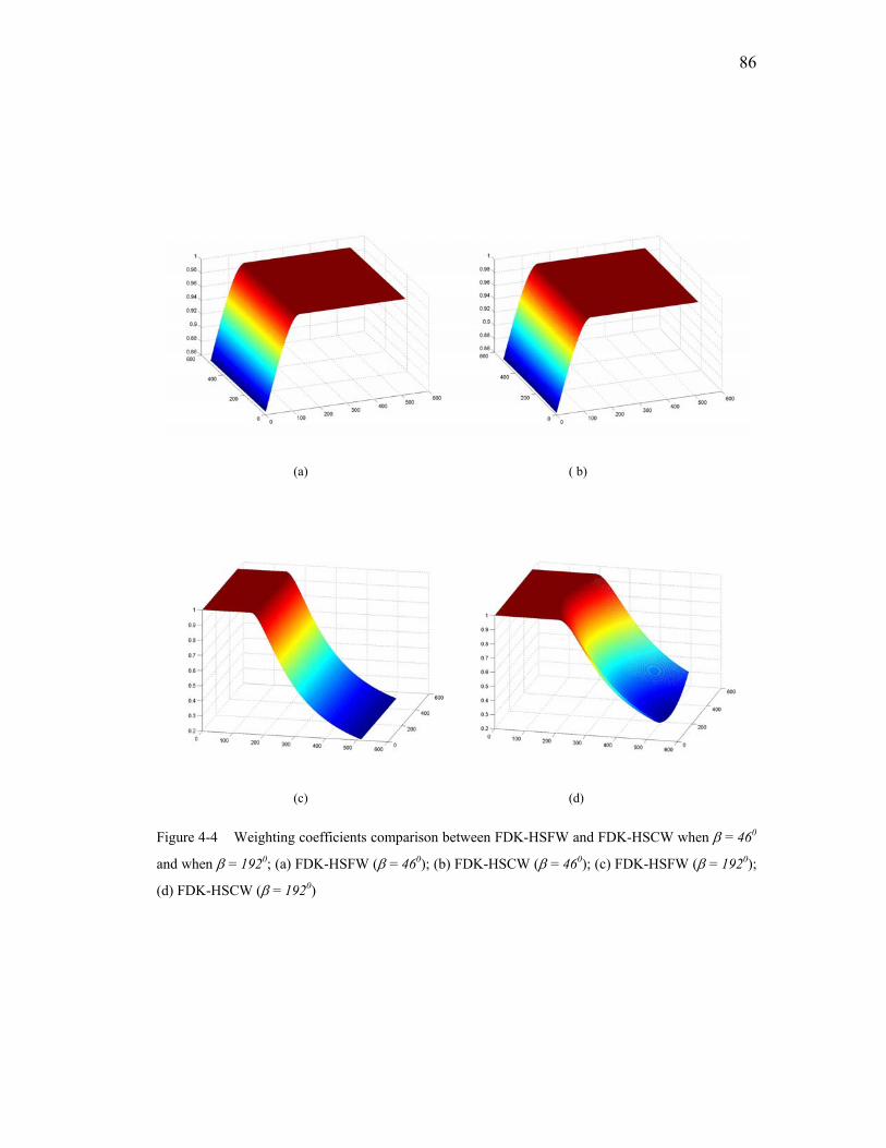
86
(a) ( b)
(c) (d)
Figure 4-4 Weighting coefficients comparison between FDK-HSFW and FDK-HSCW when β = 460
and when β = 1920; (a) FDK-HSFW (β = 460); (b) FDK-HSCW (β = 460); (c) FDK-HSFW (β = 1920);
(d) FDK-HSCW (β = 1920)

87
(a) (b)
(c) (d)
Figure 4-5 Reconstructed sagittal images from different FDK schemes at X = 0 mm; (a) FDK-FS; (b)
FDK-HSFW; (c) MFDK-HS; (d) Phantom
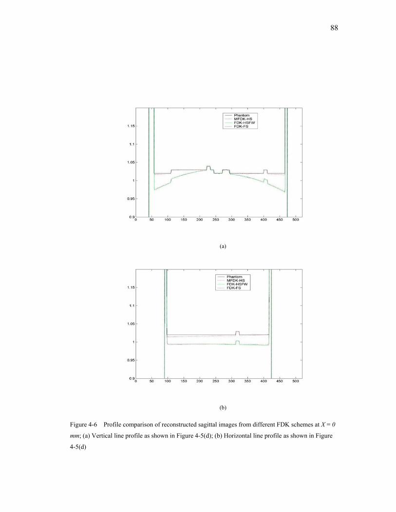
88
(a)
(b)
Figure 4-6 Profile comparison of reconstructed sagittal images from different FDK schemes at X = 0
mm; (a) Vertical line profile as shown in Figure 4-5(d); (b) Horizontal line profile as shown in Figure
4-5(d)
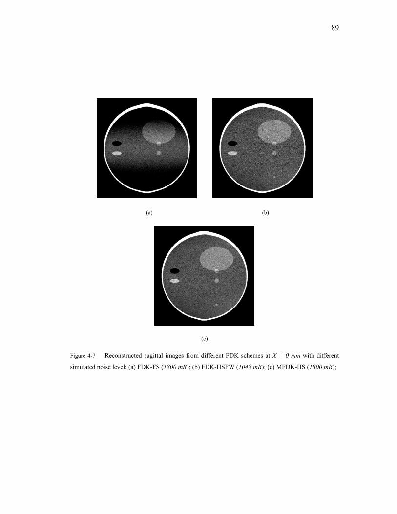
89
(a) (b)
(c)
Figure 4-7 Reconstructed sagittal images from different FDK schemes at X = 0 mm with different
simulated noise level; (a) FDK-FS (1800 mR); (b) FDK-HSFW (1048 mR); (c) MFDK-HS (1800 mR);
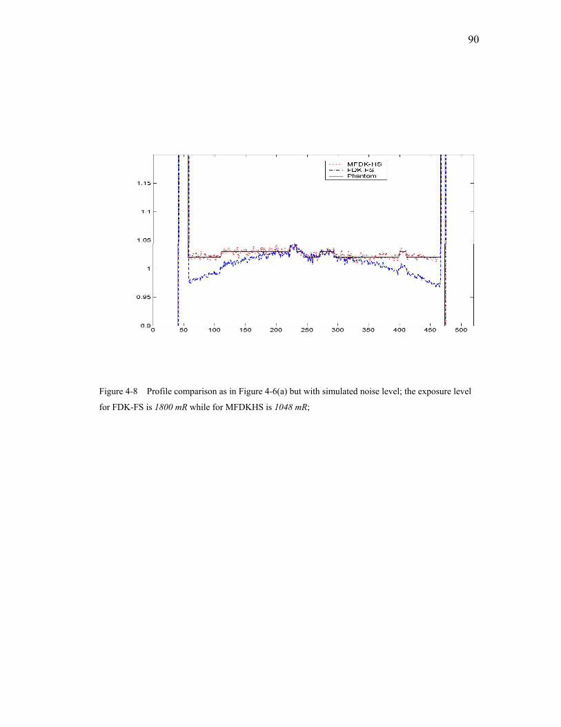
90
Figure 4-8 Profile comparison as in Figure 4-6(a) but with simulated noise level; the exposure level
for FDK-FS is 1800 mR while for MFDKHS is 1048 mR;
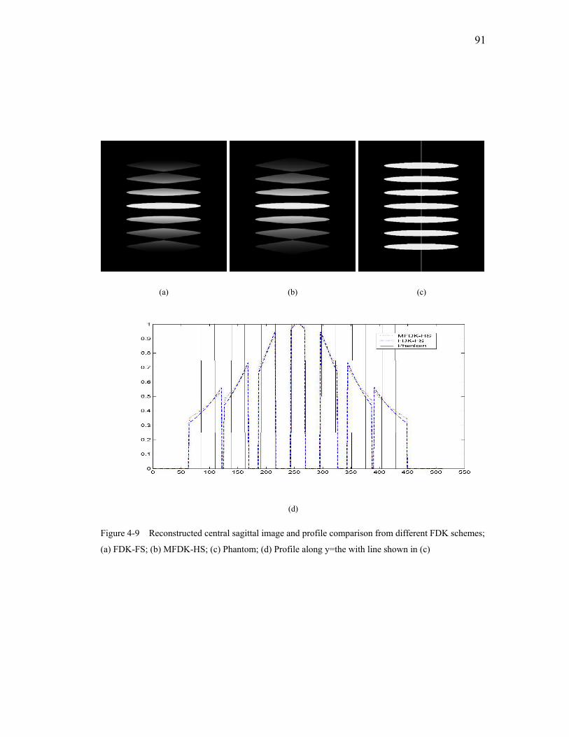
91
(a) (b) (c)
(d)
Figure 4-9 Reconstructed central sagittal image and profile comparison from different FDK schemes;
(a) FDK-FS; (b) MFDK-HS; (c) Phantom; (d) Profile along y=the with line shown in (c)
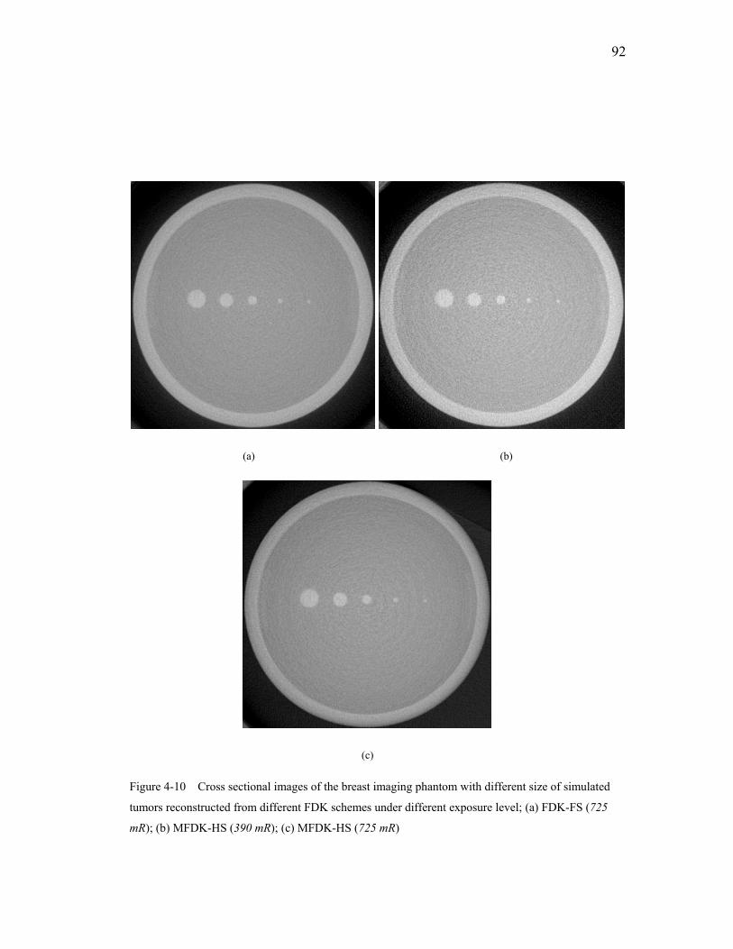
92
(a) (b)
(c)
Figure 4-10 Cross sectional images of the breast imaging phantom with different size of simulated
tumors reconstructed from different FDK schemes under different exposure level; (a) FDK-FS (725
mR); (b) MFDK-HS (390 mR); (c) MFDK-HS (725 mR)
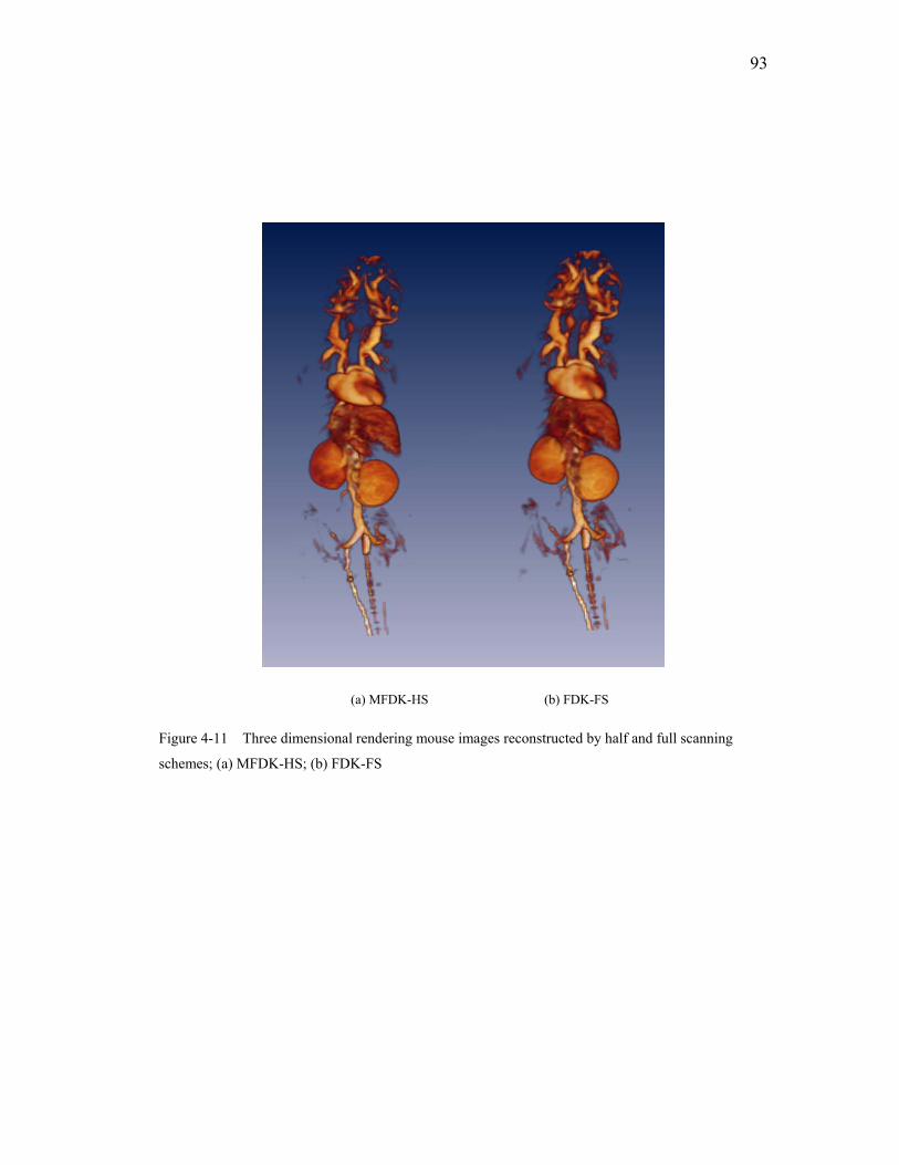
93
(a) MFDK-HS (b) FDK-FS
Figure 4-11 Three dimensional rendering mouse images reconstructed by half and full scanning
schemes; (a) MFDK-HS; (b) FDK-FS
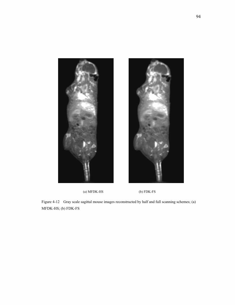
94
(a) MFDK-HS (b) FDK-FS
Figure 4-12 Gray scale sagittal mouse images reconstructed by half and full scanning schemes; (a)
MFDK-HS; (b) FDK-FS
95
Chapter 5 CBBCT Dynamic Study
5.1 Background and purpose of the dynamic study
Tumor angiogenesis is the process by which new blood vessels are formed from the
existing vessels in a tumor to promote tumor growth. Tumor angiogenesis has
important implications in the diagnosis and treatment of various solid tumors [112].
Because angiogenesis is crucial for tumor growth, tumor progression and tumor
metastasis, it can be used as a prognostic indicator to predict the outcome of the
disease and treatment. Studies of contrast-enhanced mammography have
demonstrated increased lesion conspicuity and have shown that this technique
provides information on contrast kinetics [113, 114]. It has been suggested that
malignant and benign lesions can be differentiated in part by their uptake kinetics.
Based on the above introduction, we can see that the angiogenesis study is conducted
by using functional CT to get the degree of the enhancement within tumor after
injecting the contrast agent intravenously. For typical doses of contrast material, the
amount of enhancement is proportional to the concentration of this material within the
region of interest. A series of images obtained at one location over time allows
generation of time-attenuation data from which a number of semi-quantitative
parameter, such as enhancement rate, can be determined.

96
5.2 CBBCT dynamic study based on computer
simulation
This first study is intended to give a qualitative evaluation based on computer
simulations about which scanning scheme, full-scan or half-scan can better delineate
the simulated time-intensity curve under different gantry scanning speed by utilizing
the flat panel-based Cone beam CT technology.
5.2.1 The scanning parameters associated with the computer
simulation
The scanning speed is set up with three speeds, 1 second per circle, 5 seconds per
circle and 10 seconds per circle. The breast phantom used in the simulation is a half-
ellipsoid with three half-axes of 6, 6 and 12 cm. There is a simulated ellipse tumor
inside the breast phantom. The three half-axes of this tumor are 2.5, 2.5 and 5 cm
respectively. The attenuation coefficient of the tumor is elevated as the contrast agent
flows into it. The simulated attenuation coefficient time (A-T) curve within tumor is
shown in Figure 5-1. The time-varied intensity follows the Rayleigh distribution with
an adjustable parameter to decide the time point where a peak value appears. This
parameter determines the rising up shape and tail shape. The rising up part simulates
the wash-in period, while the tail part simulates the wash-out period.
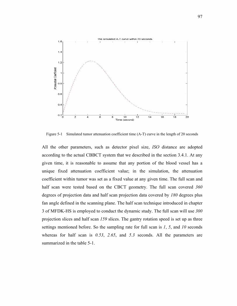
97
Figure 5-1 Simulated tumor attenuation coefficient time (A-T) curve in the length of 20 seconds
All the other parameters, such as detector pixel size, ISO distance are adopted
according to the actual CBBCT system that we described in the section 3.4.1. At any
given time, it is reasonable to assume that any portion of the blood vessel has a
unique fixed attenuation coefficient value; in the simulation, the attenuation
coefficient within tumor was set as a fixed value at any given time. The full scan and
half scan were tested based on the CBCT geometry. The full scan covered 360
degrees of projection data and half scan projection data covered by 180 degrees plus
fan angle defined in the scanning plane. The half scan technique introduced in chapter
3 of MFDK-HS is employed to conduct the dynamic study. The full scan will use 300
projection slices and half scan 159 slices. The gantry rotation speed is set up as three
settings mentioned before. So the sampling rate for full scan is 1, 5, and 10 seconds
whereas for half scan is 0.53, 2.65, and 5.3 seconds. All the parameters are
summarized in the table 5-1.
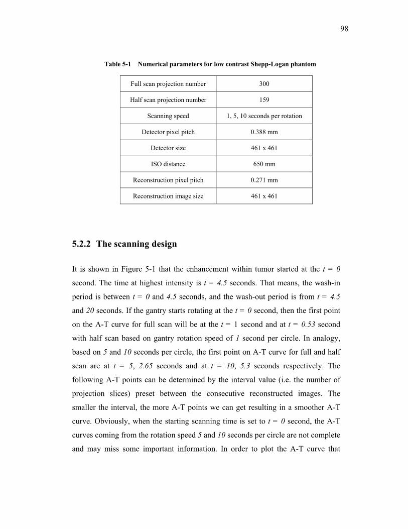
98
Table 5-1 Numerical parameters for low contrast Shepp-Logan phantom
Full scan projection number 300
Half scan projection number 159
Scanning speed 1, 5, 10 seconds per rotation
Detector pixel pitch 0.388 mm
Detector size 461 x 461
ISO distance 650 mm
Reconstruction pixel pitch 0.271 mm
Reconstruction image size 461 x 461
5.2.2 The scanning design
It is shown in Figure 5-1 that the enhancement within tumor started at the t = 0
second. The time at highest intensity is t = 4.5 seconds. That means, the wash-in
period is between t = 0 and 4.5 seconds, and the wash-out period is from t = 4.5
and 20 seconds. If the gantry starts rotating at the t = 0 second, then the first point
on the A-T curve for full scan will be at the t = 1 second and at t = 0.53 second
with half scan based on gantry rotation speed of 1 second per circle. In analogy,
based on 5 and 10 seconds per circle, the first point on A-T curve for full and half
scan are at t = 5, 2.65 seconds and at t = 10, 5.3 seconds respectively. The
following A-T points can be determined by the interval value (i.e. the number of
projection slices) preset between the consecutive reconstructed images. The
smaller the interval, the more A-T points we can get resulting in a smoother A-T
curve. Obviously, when the starting scanning time is set to t = 0 second, the A-T
curves coming from the rotation speed 5 and 10 seconds per circle are not complete
and may miss some important information. In order to plot the A-T curve that
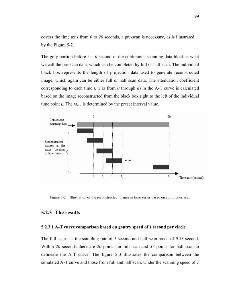
99
covers the time axis from 0 to 20 seconds, a pre-scan is necessary, as is illustrated
by the Figure 5-2.
The gray portion before t = 0 second in the continuous scanning data block is what
we call the pre-scan data, which can be completed by full or half scan. The individual
black box represents the length of projection data used to generate reconstructed
image, which again can be either full or half scan data. The attenuation coefficient
corresponding to each time ti (i is from 0 through n) in the A-T curve is calculated
based on the image reconstructed from the black box right to the left of the individual
time point ti. The titi+1 is determined by the preset interval value.
Figure 5-2 Illustration of the reconstructed images in time series based on continuous scan
5.2.3 The results
5.2.3.1 A-T curve comparison based on gantry speed of 1 second per circle
The full scan has the sampling rate of 1 second and half scan has it of 0.53 second.
Within 20 seconds there are 20 points for full scan and 37 points for half scan to
delineate the A-T curve. The figure 5-3 illustrates the comparison between the
simulated A-T curve and those from full and half scan. Under the scanning speed of 1
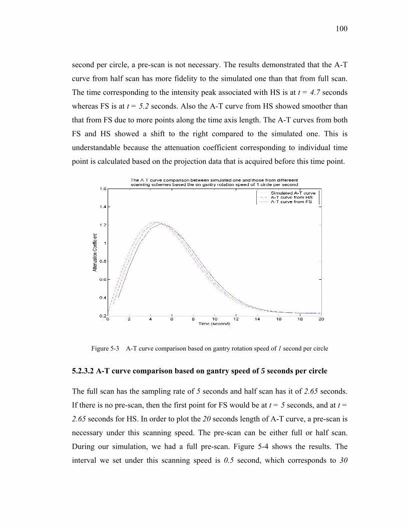
100
second per circle, a pre-scan is not necessary. The results demonstrated that the A-T
curve from half scan has more fidelity to the simulated one than that from full scan.
The time corresponding to the intensity peak associated with HS is at t = 4.7 seconds
whereas FS is at t = 5.2 seconds. Also the A-T curve from HS showed smoother than
that from FS due to more points along the time axis length. The A-T curves from both
FS and HS showed a shift to the right compared to the simulated one. This is
understandable because the attenuation coefficient corresponding to individual time
point is calculated based on the projection data that is acquired before this time point.
Figure 5-3 A-T curve comparison based on gantry rotation speed of 1 second per circle
5.2.3.2 A-T curve comparison based on gantry speed of 5 seconds per circle
The full scan has the sampling rate of 5 seconds and half scan has it of 2.65 seconds.
If there is no pre-scan, then the first point for FS would be at t = 5 seconds, and at t =
2.65 seconds for HS. In order to plot the 20 seconds length of A-T curve, a pre-scan is
necessary under this scanning speed. The pre-scan can be either full or half scan.
During our simulation, we had a full pre-scan. Figure 5-4 shows the results. The
interval we set under this scanning speed is 0.5 second, which corresponds to 30
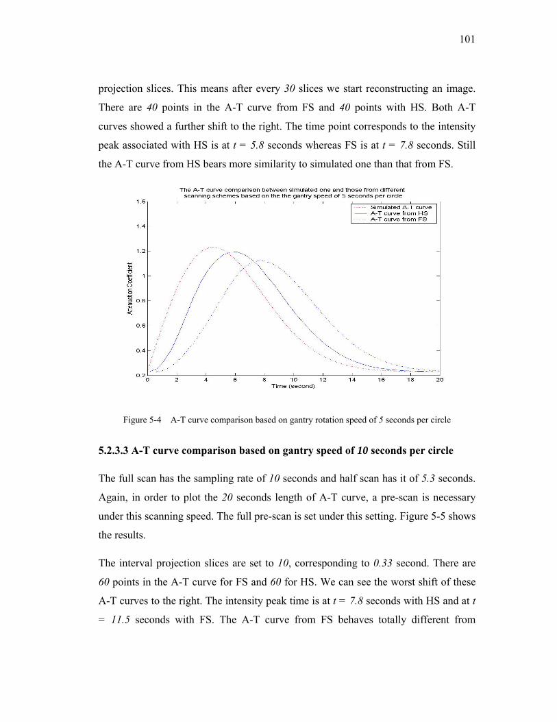
101
projection slices. This means after every 30 slices we start reconstructing an image.
There are 40 points in the A-T curve from FS and 40 points with HS. Both A-T
curves showed a further shift to the right. The time point corresponds to the intensity
peak associated with HS is at t = 5.8 seconds whereas FS is at t = 7.8 seconds. Still
the A-T curve from HS bears more similarity to simulated one than that from FS.
Figure 5-4 A-T curve comparison based on gantry rotation speed of 5 seconds per circle
5.2.3.3 A-T curve comparison based on gantry speed of 10 seconds per circle
The full scan has the sampling rate of 10 seconds and half scan has it of 5.3 seconds.
Again, in order to plot the 20 seconds length of A-T curve, a pre-scan is necessary
under this scanning speed. The full pre-scan is set under this setting. Figure 5-5 shows
the results.
The interval projection slices are set to 10, corresponding to 0.33 second. There are
60 points in the A-T curve for FS and 60 for HS. We can see the worst shift of these
A-T curves to the right. The intensity peak time is at t = 7.8 seconds with HS and at t
= 11.5 seconds with FS. The A-T curve from FS behaves totally different from
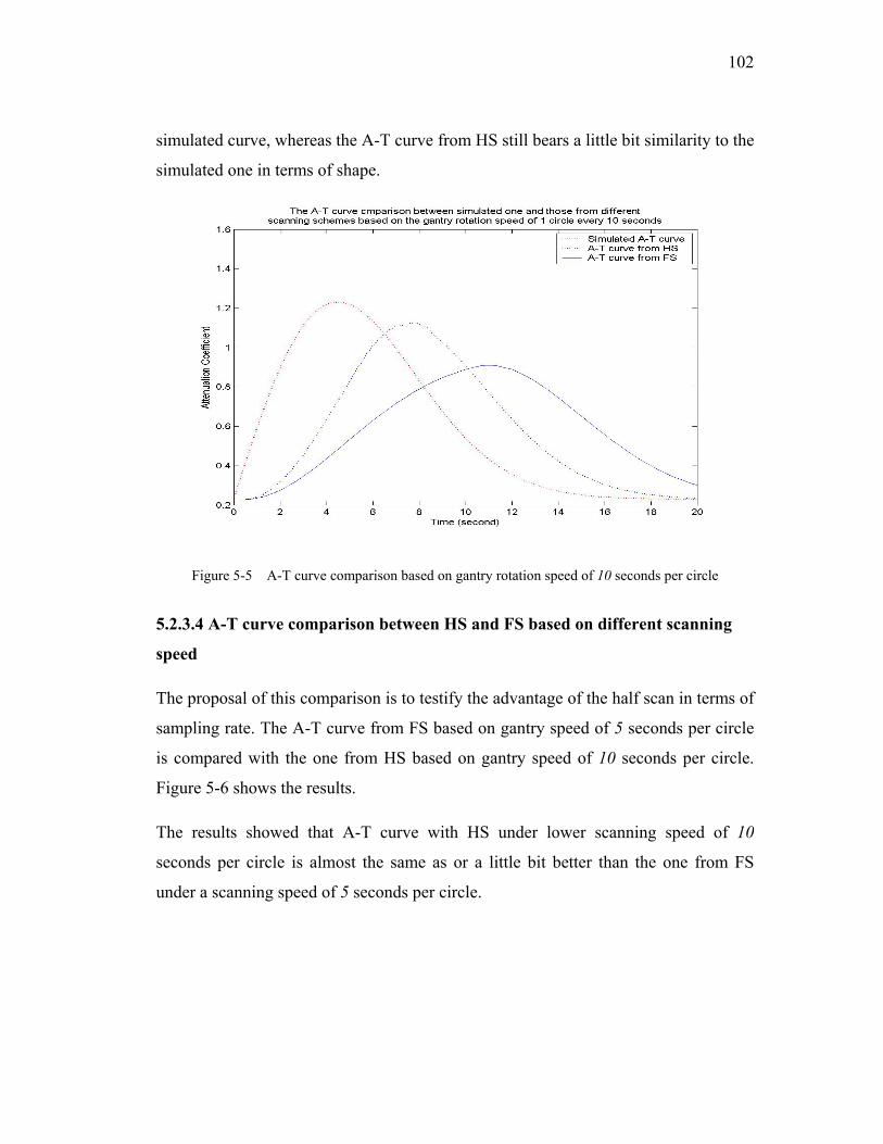
102
simulated curve, whereas the A-T curve from HS still bears a little bit similarity to the
simulated one in terms of shape.
Figure 5-5 A-T curve comparison based on gantry rotation speed of 10 seconds per circle
5.2.3.4 A-T curve comparison between HS and FS based on different scanning
speed
The proposal of this comparison is to testify the advantage of the half scan in terms of
sampling rate. The A-T curve from FS based on gantry speed of 5 seconds per circle
is compared with the one from HS based on gantry speed of 10 seconds per circle.
Figure 5-6 shows the results.
The results showed that A-T curve with HS under lower scanning speed of 10
seconds per circle is almost the same as or a little bit better than the one from FS
under a scanning speed of 5 seconds per circle.
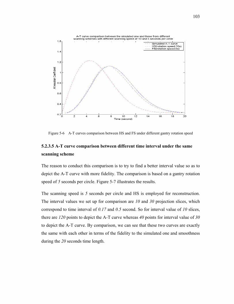
103
Figure 5-6 A-T curves comparison between HS and FS under different gantry rotation speed
5.2.3.5 A-T curve comparison between different time interval under the same
scanning scheme
The reason to conduct this comparison is to try to find a better interval value so as to
depict the A-T curve with more fidelity. The comparison is based on a gantry rotation
speed of 5 seconds per circle. Figure 5-7 illustrates the results.
The scanning speed is 5 seconds per circle and HS is employed for reconstruction.
The interval values we set up for comparison are 10 and 30 projection slices, which
correspond to time interval of 0.17 and 0.5 second. So for interval value of 10 slices,
there are 120 points to depict the A-T curve whereas 40 points for interval value of 30
to depict the A-T curve. By comparison, we can see that these two curves are exactly
the same with each other in terms of the fidelity to the simulated one and smoothness
during the 20 seconds time length.
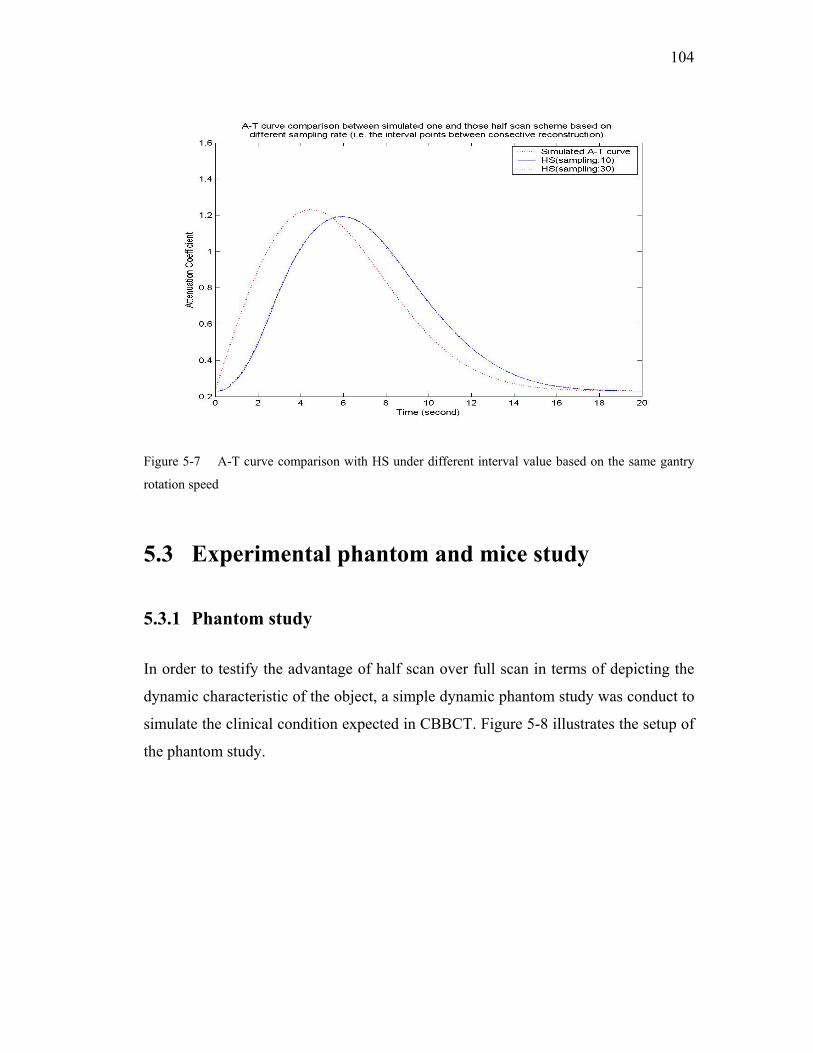
104
Figure 5-7 A-T curve comparison with HS under different interval value based on the same gantry
rotation speed
5.3 Experimental phantom and mice study
5.3.1 Phantom study
In order to testify the advantage of half scan over full scan in terms of depicting the
dynamic characteristic of the object, a simple dynamic phantom study was conduct to
simulate the clinical condition expected in CBBCT. Figure 5-8 illustrates the setup of
the phantom study.
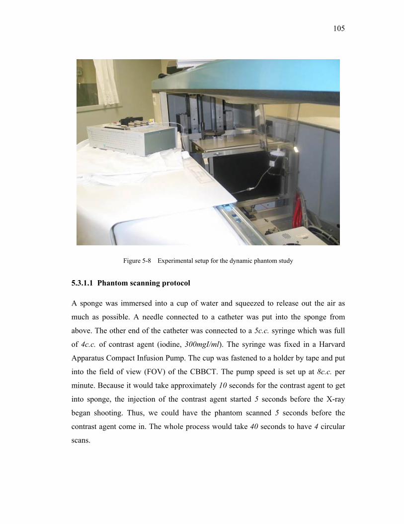
105
Figure 5-8 Experimental setup for the dynamic phantom study
5.3.1.1 Phantom scanning protocol
A sponge was immersed into a cup of water and squeezed to release out the air as
much as possible. A needle connected to a catheter was put into the sponge from
above. The other end of the catheter was connected to a 5c.c. syringe which was full
of 4c.c. of contrast agent (iodine, 300mgI/ml). The syringe was fixed in a Harvard
Apparatus Compact Infusion Pump. The cup was fastened to a holder by tape and put
into the field of view (FOV) of the CBBCT. The pump speed is set up at 8c.c. per
minute. Because it would take approximately 10 seconds for the contrast agent to get
into sponge, the injection of the contrast agent started 5 seconds before the X-ray
began shooting. Thus, we could have the phantom scanned 5 seconds before the
contrast agent come in. The whole process would take 40 seconds to have 4 circular
scans.
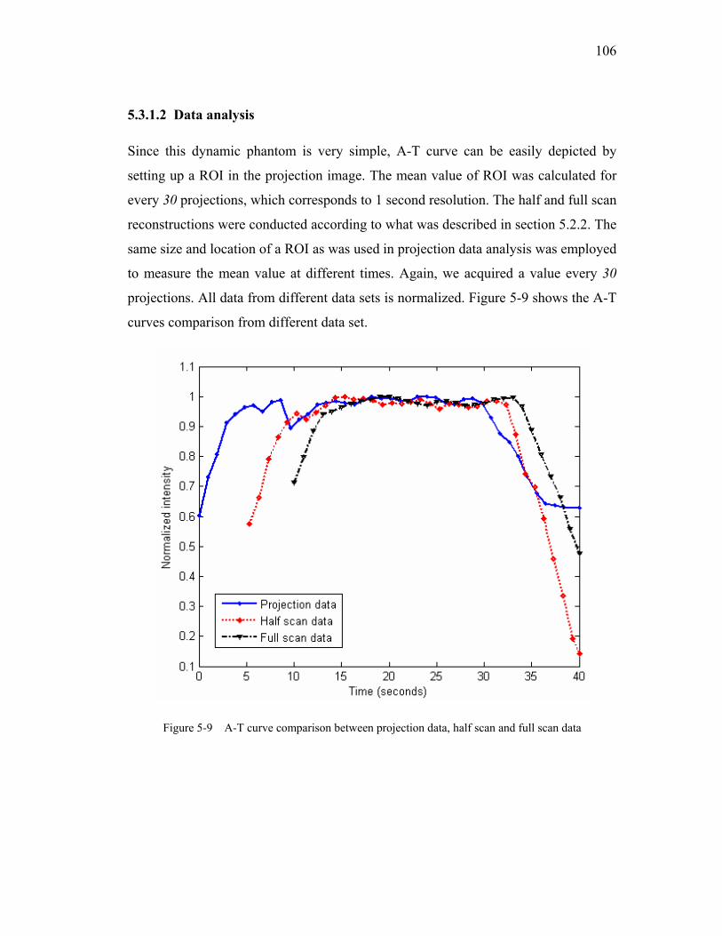
106
5.3.1.2 Data analysis
Since this dynamic phantom is very simple, A-T curve can be easily depicted by
setting up a ROI in the projection image. The mean value of ROI was calculated for
every 30 projections, which corresponds to 1 second resolution. The half and full scan
reconstructions were conducted according to what was described in section 5.2.2. The
same size and location of a ROI as was used in projection data analysis was employed
to measure the mean value at different times. Again, we acquired a value every 30
projections. All data from different data sets is normalized. Figure 5-9 shows the A-T
curves comparison from different data set.
Figure 5-9 A-T curve comparison between projection data, half scan and full scan data
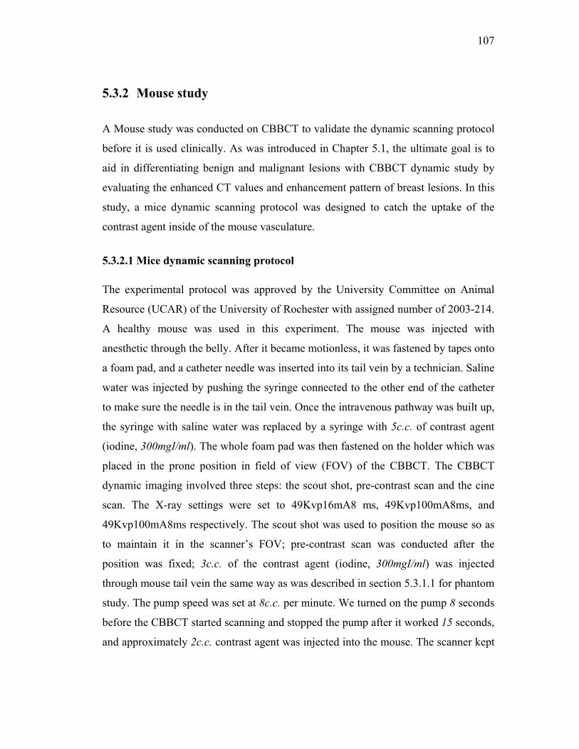
107
5.3.2 Mouse study
A Mouse study was conducted on CBBCT to validate the dynamic scanning protocol
before it is used clinically. As was introduced in Chapter 5.1, the ultimate goal is to
aid in differentiating benign and malignant lesions with CBBCT dynamic study by
evaluating the enhanced CT values and enhancement pattern of breast lesions. In this
study, a mice dynamic scanning protocol was designed to catch the uptake of the
contrast agent inside of the mouse vasculature.
5.3.2.1 Mice dynamic scanning protocol
The experimental protocol was approved by the University Committee on Animal
Resource (UCAR) of the University of Rochester with assigned number of 2003-214.
A healthy mouse was used in this experiment. The mouse was injected with
anesthetic through the belly. After it became motionless, it was fastened by tapes onto
a foam pad, and a catheter needle was inserted into its tail vein by a technician. Saline
water was injected by pushing the syringe connected to the other end of the catheter
to make sure the needle is in the tail vein. Once the intravenous pathway was built up,
the syringe with saline water was replaced by a syringe with 5c.c. of contrast agent
(iodine, 300mgI/ml). The whole foam pad was then fastened on the holder which was
placed in the prone position in field of view (FOV) of the CBBCT. The CBBCT
dynamic imaging involved three steps: the scout shot, pre-contrast scan and the cine
scan. The X-ray settings were set to 49Kvp16mA8 ms, 49Kvp100mA8ms, and
49Kvp100mA8ms respectively. The scout shot was used to position the mouse so as
to maintain it in the scanner’s FOV; pre-contrast scan was conducted after the
position was fixed; 3c.c. of the contrast agent (iodine, 300mgI/ml) was injected
through mouse tail vein the same way as was described in section 5.3.1.1 for phantom
study. The pump speed was set at 8c.c. per minute. We turned on the pump 8 seconds
before the CBBCT started scanning and stopped the pump after it worked 15 seconds,
and approximately 2c.c. contrast agent was injected into the mouse. The scanner kept
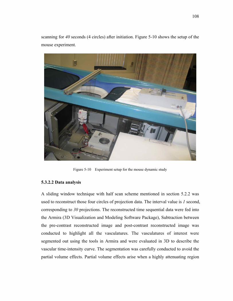
108
scanning for 40 seconds (4 circles) after initiation. Figure 5-10 shows the setup of the
mouse experiment.
Figure 5-10 Experiment setup for the mouse dynamic study
5.3.2.2 Data analysis
A sliding window technique with half scan scheme mentioned in section 5.2.2 was
used to reconstruct those four circles of projection data. The interval value is 1 second,
corresponding to 30 projections. The reconstructed time sequential data were fed into
the Armira (3D Visualization and Modeling Software Package), Subtraction between
the pre-contrast reconstructed image and post-contrast reconstructed image was
conducted to highlight all the vasculatures. The vasculatures of interest were
segmented out using the tools in Armira and were evaluated in 3D to describe the
vascular time-intensity curve. The segmentation was carefully conducted to avoid the
partial volume effects. Partial volume effects arise when a highly attenuating region
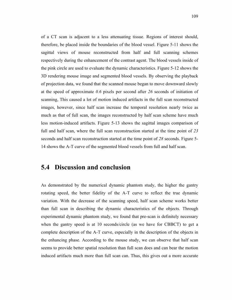
109
of a CT scan is adjacent to a less attenuating tissue. Regions of interest should,
therefore, be placed inside the boundaries of the blood vessel. Figure 5-11 shows the
sagittal views of mouse reconstructed from half and full scanning schemes
respectively during the enhancement of the contrast agent. The blood vessels inside of
the pink circle are used to evaluate the dynamic characteristics. Figure 5-12 shows the
3D rendering mouse image and segmented blood vessels. By observing the playback
of projection data, we found that the scanned mouse began to move downward slowly
at the speed of approximate 0.6 pixels per second after 26 seconds of initiation of
scanning, This caused a lot of motion induced artifacts in the full scan reconstructed
images, however, since half scan increase the temporal resolution nearly twice as
much as that of full scan, the images reconstructed by half scan scheme have much
less motion-induced artifacts. Figure 5-13 shows the sagittal images comparison of
full and half scan, where the full scan reconstruction started at the time point of 23
seconds and half scan reconstruction started at the time point of 28 seconds. Figure 5-
14 shows the A-T curve of the segmented blood vessels from full and half scan.
5.4 Discussion and conclusion
As demonstrated by the numerical dynamic phantom study, the higher the gantry
rotating speed, the better fidelity of the A-T curve to reflect the true dynamic
variation. With the decrease of the scanning speed, half scan scheme works better
than full scan in describing the dynamic characteristics of the objects. Through
experimental dynamic phantom study, we found that pre-scan is definitely necessary
when the gantry speed is at 10 seconds/circle (as we have for CBBCT) to get a
complete description of the A-T curve, especially in the description of the objects in
the enhancing phase. According to the mouse study, we can observe that half scan
seems to provide better spatial resolution than full scan does and can bear the motion
induced artifacts much more than full scan can. Thus, this gives out a more accurate
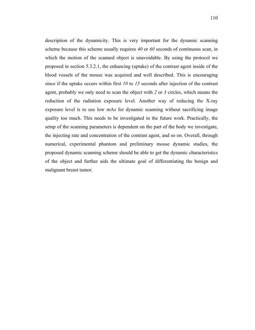
110
description of the dynamicity. This is very important for the dynamic scanning
scheme because this scheme usually requires 40 or 60 seconds of continuous scan, in
which the motion of the scanned object is unavoidable. By using the protocol we
proposed in section 5.3.2.1, the enhancing (uptake) of the contrast agent inside of the
blood vessels of the mouse was acquired and well described. This is encouraging
since if the uptake occurs within first 10 to 15 seconds after injection of the contrast
agent, probably we only need to scan the object with 2 or 3 circles, which means the
reduction of the radiation exposure level. Another way of reducing the X-ray
exposure level is to use low mAs for dynamic scanning without sacrificing image
quality too much. This needs to be investigated in the future work. Practically, the
setup of the scanning parameters is dependent on the part of the body we investigate,
the injecting rate and concentration of the contrast agent, and so on. Overall, through
numerical, experimental phantom and preliminary mouse dynamic studies, the
proposed dynamic scanning scheme should be able to get the dynamic characteristics
of the object and further aids the ultimate goal of differentiating the benign and
malignant breast tumor.
111
(a) (b)
Figure 5-11 Sagittal images of the reconstructed mouse from different FDK schemes; (a) FDK-FS ( # of
projections = 300); (b) MFDK-HS ( # of projections = 160)
112
(a)
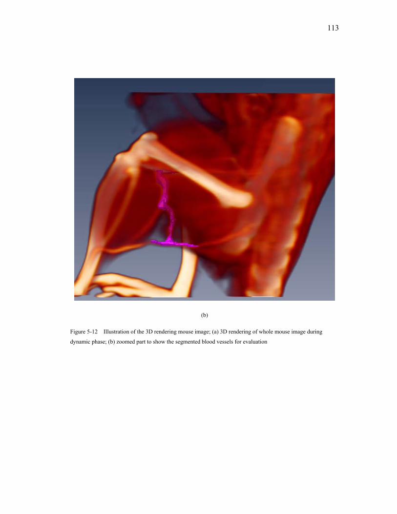
113
(b)
Figure 5-12 Illustration of the 3D rendering mouse image; (a) 3D rendering of whole mouse image during
dynamic phase; (b) zoomed part to show the segmented blood vessels for evaluation
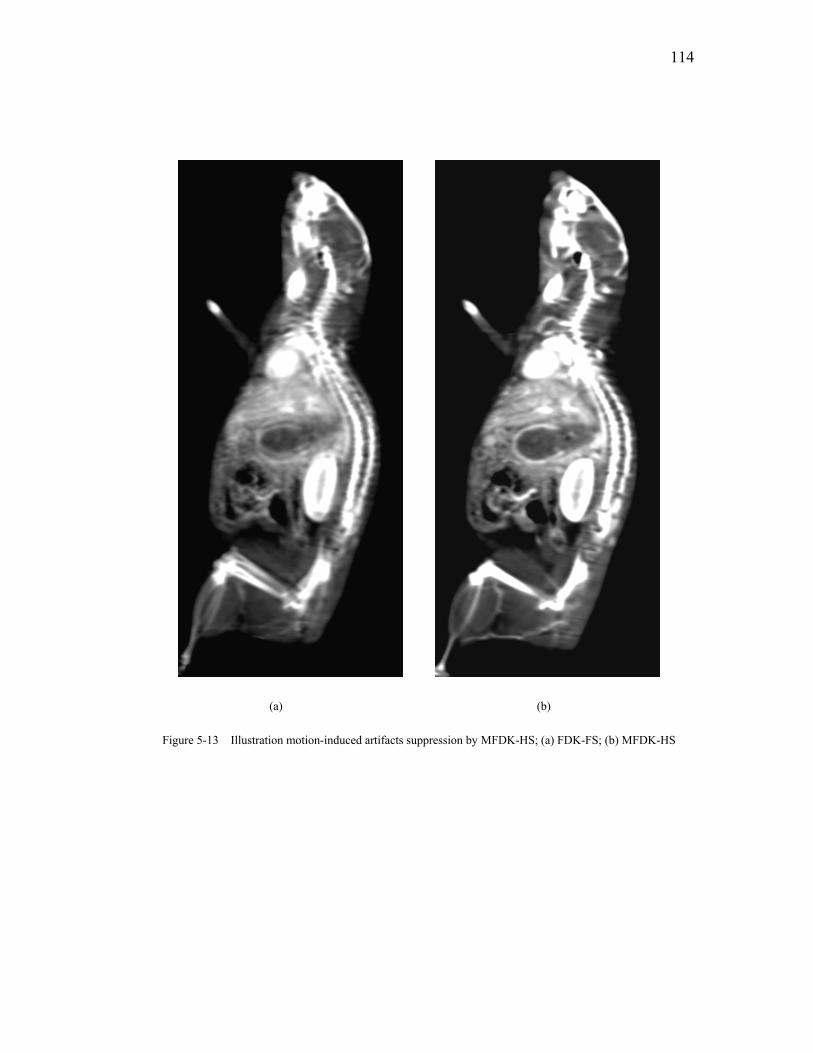
114
(a) (b)
Figure 5-13 Illustration motion-induced artifacts suppression by MFDK-HS; (a) FDK-FS; (b) MFDK-HS
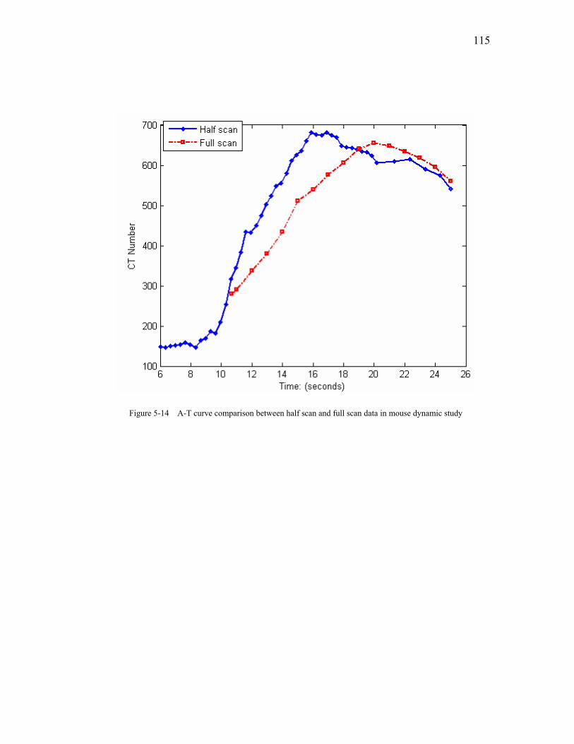
115
Figure 5-14 A-T curve comparison between half scan and full scan data in mouse dynamic study
116
Chapter 6 Summary and future work
6.1 Summary
As long as the circular scanning trajectory is involved for CBCT system, FDK is by
far the best algorithm for an approximate reconstruction of the object within the limit
of the acceptable scanning cone angle based on the geometrical scanning parameters.
When the scanning is conducted beyond the acceptable scanning cone angle, a
supplementary scanning trajectory and an efficient reconstruction algorithm
associated with this trajectory are necessary to compensate the artifacts such as
density drop along the scanning axis and reconstructed object deformation further
away from the scanning plane caused only by the single circle scan. In this thesis, a
novel circle plus partial helical line scanning scheme was proposed to correct the
aforementioned artifacts. Computer numerical simulations and breast phantom
experimental studies validated the accuracy of this new scanning scheme over the
single circle scan. The partial helical scanning trajectory is aimed at correcting the
artifacts induced by single circle scan to get the clinically acceptable images and not
for an exact reconstruction. The image quality associated with the proposed circle
plus partial helical line scanning scheme is close to the one from exact reconstruction
which was also conducted through numerical simulation by relaxing the restrictions
required by the exact scanning scheme. However the number of x-ray shoots with
circle plus partial helical line scheme is much smaller than that of the exact scanning
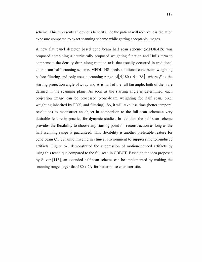
117
scheme. This represents an obvious benefit since the patient will receive less radiation
exposure compared to exact scanning scheme while getting acceptable images.
A new flat panel detector based cone beam half scan scheme (MFDK-HS) was
proposed combining a heuristically proposed weighting function and Hui’s term to
compensate the density drop along rotation axis that usually occurred in traditional
cone beam half scanning scheme. MFDK-HS needs additional cone-beam weighting
before filtering and only uses a scanning range of [ ]Δ++ 2180, ββ , where β is the
starting projection angle of x-ray and Δ is half of the full fan angle; both of them are
defined in the scanning plane. As soon as the starting angle is determined, each
projection image can be processed (cone-beam weighting for half scan, pixel
weighting inherited by FDK, and filtering). So, it will take less time (better temporal
resolution) to reconstruct an object in comparison to the full scan scheme-a very
desirable feature in practice for dynamic studies. In addition, the half-scan scheme
provides the flexibility to choose any starting point for reconstruction as long as the
half scanning range is guaranteed. This flexibility is another preferable feature for
cone beam CT dynamic imaging in clinical environment to suppress motion-induced
artifacts. Figure 6-1 demonstrated the suppression of motion-induced artifacts by
using this technique compared to the full scan in CBBCT. Based on the idea proposed
by Silver [115], an extended half-scan scheme can be implemented by making the
scanning range larger than Δ+ 2180 for better noise characteristic.
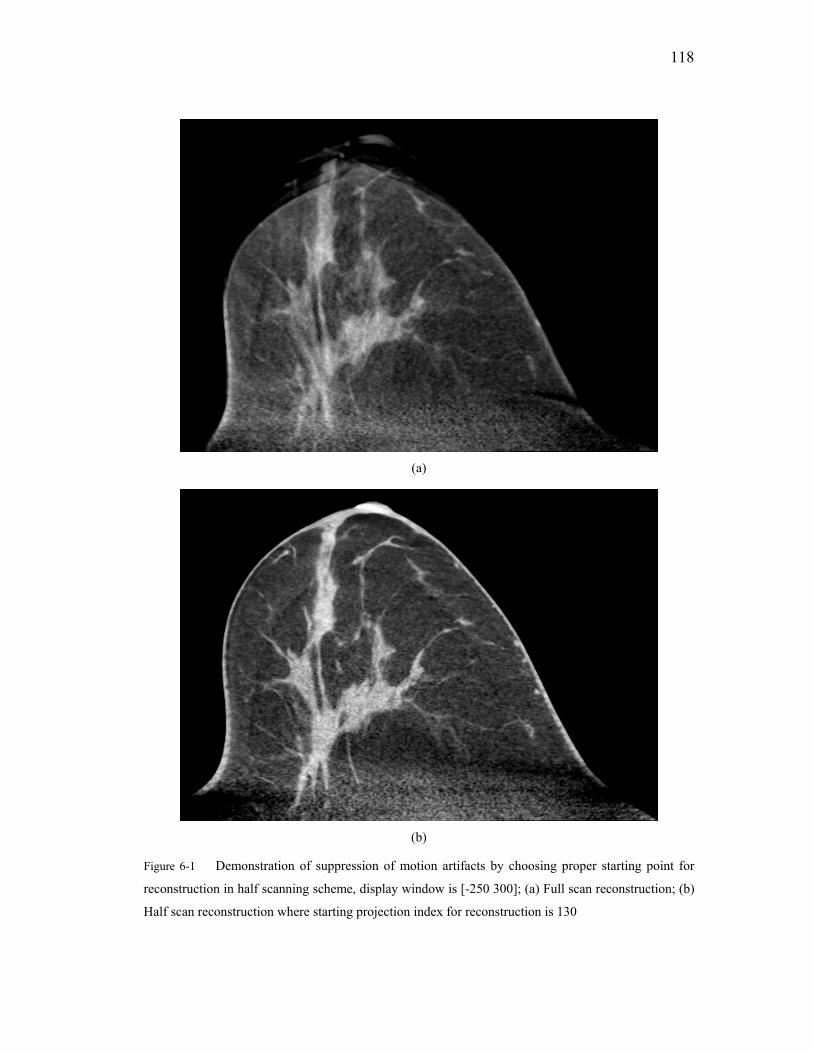
118
(a)
(b)
Figure 6-1 Demonstration of suppression of motion artifacts by choosing proper starting point for
reconstruction in half scanning scheme, display window is [-250 300]; (a) Full scan reconstruction; (b)
Half scan reconstruction where starting projection index for reconstruction is 130
119
A preliminary dynamic study using CBBCT was conducted in our Lab. Through a
computer numerical dynamic phantom, an experimental dynamic phantom and a mice
study, a dynamic scanning protocol employing the cone beam half scanning scheme
was established. Results showed that the half scanning scheme works much better
than full scanning scheme in terms of better description of the dynamic characteristics
of the object and suppression of motion-induced artifacts. The proposed scanning
protocol could be used to delineate the uptake (the rising) enhancement curve which
is very important to potentially differentiate between the benign and malignant
tumors.
6.2 Future work
6.2.1 Patient dynamic study
CBCT dynamic study is an exciting application area due to the high time and spatial
resolution, and true 3D isotropic characteristics possessed by the CBCT. A patient
dynamic study on CBBCT will be conducted soon based on the studies we did on
phantoms and mouse. Considering the different dynamic characteristics associated
with different organs, the setup of the scanning protocol should be object-dependent.
6.2.2 De-noising and improvement of spatial resolution
As was illustrated in Chapter 4, half scan did increase the noise level compared to full
scan. If the same contrast to noise ratio is desired for both half and full scan (the total
exposure level for both cases is same), the exposure level per projection associated
with the half scan has to be increased. Another way to keep approximately the same
contrast to noise ratio for both cases without increasing the exposure level per
projection for half scan is to do the de-noising on the projection data. Traditionally,
noise suppression employs a window such as Shepp-Logan, Hamming and cosine in
120
addition to the ramp linear filter as was described in Chapter 2. This was achieved by
sacrificing the spatial resolution. In order for the half scan to have approximate the
same noise level as full scan, windows with more noise suppression would be
enrolled which result in poorer spatial resolution as compared to the full scan. As was
indicated in Chapter 2, the best spatial resolution in the reconstructed image would be
achieved by employing the ramp linear filter. Based on the aforementioned
introduction, which is a common phenomenon resulted from the linear filter operation,
exploring the problems of how to maintain the spatial resolution and to reduce noise
as much as possible in the domain other than Fourier domain, might be a way to
achieve this purpose. Signal de-noising in Wavelet domain is a promising area in the
past decade. Wavelet coefficients shrinkage is one of the most efficient ways to deal
with a de-nosing problem. It is possible for them to suppress the additive noises while
keeping signals previously degraded by low-pass filters [116].
121
Papers and patent related to this thesis
[ 1 ] D. Yang, R. Ning, “FDK Half-scan with a heuristic weighting scheme on a flat panel detector-based Cone Beam CT (FDK-HSCW),” International Journal of Biomedical Imaging, vol. 2006, Article ID 83983, 8 pages, 2006.
[ 2 ] D. Yang, R. Ning, “Circle plus partial helical scan scheme based on a flat panel detector for Cone Beam Breast X-ray CT (CBBCT),” Resubmitted for IEEE Transaction on Medical Imaging after revision.
[ 3 ] D. Yang, R. Ning, S. Liu, D. Conover, “Implementation and evaluation of 4D cone beam CT (CBCT) reconstruction,” Proc. SPIE Med. Imaging 6510, pp. 65105T1-8, 2007.
[ 4 ] R. Ning, D. L. Conover, D. Yang, Y. Yu, W. Cai, X. Lu, “Flat panel detector-based cone beam CT for dynamic imaging: system evaluation,” Proc. SPIE Med. Imaging 6142, pp. 61422C1-7, 2006.
[ 5 ] W. Cai, R. Ning, D. Yang, “Computer simulation of FDK reconstruction with the in-line holographic projection data,” Proc. SPIE Med. Imaging 6142, pp. 61424G1-10, 2006.
[ 6 ] D. Yang, R. Ning, D. L. Conover, Y. Yu, “Reconstruction implementation based on a flat panel detector cone-beam breast imaging CT (CBCTBI),” Proc. SPIE Med. Imaging 6142, pp. 61424H1-8, 2006.
[ 7 ] D. Yang, R. Ning, Y. Yu, D. L. Conover, X. Lu, “Modified FDK half-scan (MFDKHS) scheme on flat panel detector-based cone-beam CT,” Proc. SPIE Med. Imaging 5745, pp. 1030-1037, 2005.
[ 8 ] D. Yang, R. Ning, D. Conover, Y. Yu, “Half-scan Scheme with newly Developed Weighting Function on a Flat Panel Detector-based Cone –Beam CT: Phantom Studies,” Oral presentation in RSNA (2004, Chicago), The Radiological Society of North America 90th Scientific Assembly and Annual Meeting.
[ 9 ] D. Yang, R. Ning, Y. Yu, D. L. Conover, X. Lu, “Implementation & Evaluation of the Half-Scan scheme Based on CBCT (Cone-Beam CT) system,” Proc. SPIE Med. Imaging 5368, pp. 542-551, 2004.

122
[ 10 ] D. Yang, R. Ning, B. Ricardo, S. Liu, D. L. Conover, “Cone Beam CT tumor vasculature dynamic study (murine model),” Accepted for SPIE Med. Imaging 2008.
[ 11 ] Ruola Ning, Dong Yang, Method and apparatus for cone beam CT dynamic imaging, US Provisional Patent Application # 11/711,155, filed on Jan. 2007, Pending.
123
Bibliography
[ 1 ] J. Radon, “Über die bestimmung von funktionen durch ihre intergralwerte la¨ngs gewisser mannigfaltikeiten,” Ber. Sa¨chsische Akad. Wiss. 1917; 69,262–278.
[ 2 ] Hounsfield GN. Nobel Award address: computed medical imaging. Med Phys 1980; 7:283-290.
[ 3 ] Beck TJ, “CT technology overview: state of the art and future directions. In: Gould RG, Boone JM, eds. Syllabus: a categorical course in physics-technology updata and quality improvement of diagnostic x-ray imaging equipment,” Oak Brook, Ill: Radiological Society Of North America, 1996; 161-172.
[ 4 ] Fishman EK, Magid D, Ney DR, et al, “Three-dimensional imaging,” Radiology 1991; 181:321-337.
[ 5 ] Kalender WA, Seissler W, Klotz E, Vock P, “Spiral volumetric CT with single-breath-hold technique, continuous transport, and continuous scanner rotation,” Radiology 1990; 176: 181-183.
[ 6 ] Kalender W, “Thin-section three-dimensional spiral CT: is isotropic imaging possible?” Radiology 1995; 197:578-580.
[ 7 ] Klingenbeck-Regn K, Schaller S, Flohr T, Ohnesorge B, Kopp AF, Baum U, “Subsecond multi-slice computed tomography: basics and applications,” Eur J Radiol 1999; 31:110-124.
[ 8 ] Hu H, He HD, Foley WD, Fox SH, “Four multidetector-row helical CT: imgae quality and volume coverage speed,” Radiology 2000; 215:55-62.
[ 9 ] T. G. Flohr, K. Stierstorfer, S. Ulzheimer, H. Bruder, et al, “Image reconstruction and image quality evaluation for a 64-slice CT scanner with z-flying focal spot,” Med. Phys. 2005; vol. 32, pp 2536-2547.
[ 10 ] Shinichiro Mori, Masahiro Endo, Takanori Tsunoo, et al, “Physical performance evaluation of a 256-slice CT-scanner for four-dimensional imaging,” Med. Phys. 2004; vol. 31, pp 1348-1356.
[ 11 ] Chisato Kondo, Shinichiro Mori, Masahiro Endo, et al, “Real-Time Volumetric Imaging of Human Heart Without Electrocardiographic Gating by
124
256-Detector Row Computed Tomography,” J Comput Assist Tomogr. 2005; vol. 29, pp 694-698.
[ 12 ] B. Chen, R. Ning, “Cone-beam volume CT breast imaging: Feasibility study,” Med. Phys. 2002; Vol. 29, pp. 755-770.
[ 13 ] N. A. Bailey, R. A. Keller, C. V. Jakowatz, and A. C. Kak, “The capability of fluoroscopic systems for the production of computerized axial tomograms,” Invest. Radiol. 1976; 11:434-439.
[ 14 ] S. Duinker, R. J. Geluk, and H. Mulder, “Transaxial analogue tomography,” Oldelft Sci. Eng. 1980; 1:448-453.
[ 15 ] R. M. Harrison and F. T. Farmer, “The determination of anatomical cross sections using a radiotherapy simulator,” Br. J. Radiol. 1978; 59:41-66.
[ 16 ] C. J. Kotre, R. M. Harrison, and W. M. Ross, “A simulator-based CT system for radiotherapy treatment planning,” Br. J. Radiol. 1984; 57:631-635.
[ 17 ] A. T. Redpath, D. H. Wright, “The use of a simulator and treatment planning computer as a CT scanner for radiotherapy planning,” In: Proceedings of the International Conference on the Use of Computers in Radiotherapy., 1984:281-287
[ 18 ] E. L. Ritman, R. A. Robb, and L. D. Harris, “Imaging Physiological Functions: Experience with the DSR,” Philadelphia: Prager Publishers, 1985.
[ 19 ] R. Ning, R. A. Kruger, “Computer simulation of imaging intensifier-based CT detector: vascular application,” Med. Phys. 1987; 15: 188-192.
[ 20 ] R. Ning, R. A. Kruger, H. Hu, “Image intensifier-based CT volume imager for angiography,” SPIE Proc. 1988; 914: 282-287.
[ 21 ] R. Ning, R. A. Kruger, and H. Hu, “Image intensifier-based CT volume imager: angiographic application,” SPIE Proc. 1990; 1233: 285-299.
[ 22 ] R. Ning, J. Riek, and D. L. Conover, “An image intensifier-based CT volume tomographic angiography imaging system: work in progress,” SPIE Proc. 1993; 1896: 145-155.
[ 23 ] R. Ning, X. Wang, J. Shen, and D. L. Conover, “An image intensifier-based CT volume tomographic angiography imaging system: system in evaluation,” SPIE Proc. 1995; 2432: 280-291.
125
[ 24 ] R. Ning, D. Zhang, X. Wang, and D. L. Conover, “An image intensifier-based CT volume tomographic angiography imaging system: work in progress,” SPIE Proc. 1996; 2708: 328-339.
[ 25 ] R. Ning, X. Wang, D. L. Conover, and X. Tang, “An image intensifier-based CT volume tomographic angiography imaging system,” SPIE Proc. 1997; 3032: 238-246.
[ 26 ] R. Ning, D. Lee, X. Tang, et al, “Selenium Flat Panel Detector-based Volume Tomographic Angiography Imaging: Phantom Studies,” SPIE Proc. 1997; 3336: 316-324.
[ 27 ] X. Tang, R. Ning, R. Yu, and D. Conover, “A 2D Wavelet-analysis-based Calibration Technique for Flat panel Imaging Detector: Application in Cone Beam Volume CT,” SPIE Proc. 1999; 3596: 806-816.
[ 28 ] R. Ning, X. Tang, R. Yu, and D. Conover, “Flat-panel-detector-based cone beam volume CT imaging: detector evaluation,” SPIE Proc. 1999; 3659: 192-203.
[ 29 ] D. A. Jaffray, J. H. Siewerdsen, and D. G. Drake, “Performance of a volumetric CT scanner based upon a flat-panel imager,” SPIE Proc. 1999; 3569: 316-324.
[ 30 ] J. H. Siewerdsen, D. A. Jaffray, “ Cone-beam computed tomography with a flat-panel imager: Effects of image lag,” Med. Phys. 1999; 26: 2635-2647.
[ 31 ] J. H. Siewerdsen, D. A. Jaffray, “Cone-beam CT with a flat-panel imager: Noise consideration for fully 3-D computed tomography,” SPIE Proc. 2000; 3977: 408-416.
[ 32 ] R, Ning, B. Chen, R. Yu, D. Conover, X. Tang, and Y. Ning, “Flat Panel Detector-Based Cone-Beam Volume CT Angiography Imaging: System Evaluation,” IEEE Trans. Med. Imag., 2000; 19: 949-963.
[ 33 ] R. Ning, B. Chen, D. L. Conover, and R. Yu, “Flat-panel detector-based cone beam volume CT mammography imaging: preliminary phantom study,” SPIE Proc. 2001; 4320: 408-416.
[ 34 ] D. A. Jaffray, J. H. Siewerdsen, J. W. Wong, and A. A. Martinez, “Flat-panel cone-beam computed tomography for image-guide radiation therapy,” Int. J. Radiation Oncology Biol. Phys., 2002; 53: 1337-1349.
126
[ 35 ] R. Ning, D. Conover, Y. Yu, W. Cai, and X. Lu, “Flat panel detector-based cone beam CT lung imaging: Preliminary system evaluation,” SPIE Proc, 2005; 5745: 147-158.
[ 36 ] D. L. Conover, R. Ning, Y. Yu, X. Lu, R. Wood, J. Reeder, and A. Johnson, “Small animal imaging using a flat panel-based cone beam computed tomography (FPD-CBCT) imaging system,” SPIE Proc, 2005; 5745: 307-319.
[ 37 ] R. Ning, D. Conover, X. Lu, Y. Zhang, Y. Yu, L. Schiffhauer, and J. Cullinan, “Evaluation of flat panel detector-based cone beam CT breast imaging with different sizes of breast phantoms,” SPIE Proc, 2005; 5745: 626-636.
[ 38 ] R. Ning, D. Conover, Y. Yu, Y. Zhang, W. Cai, D. Yang, and X. Lu, “Flat panel detector-based cone beam CT for dynamic imaging: system evaluation”, SPIE Proc, 2006 [6142-84].
[ 39 ] J. M. Boone, A. L. C. Kwan, T. R. Nelson, et al, “Performance assessment of a pendant-geometry CT scanner for breast cancer detection,” SPIE Proc, 2004; 5745: 319-323.
[ 40 ] R. Ning, D. Conover, Y. Yu, K. Willison, L. Shiffhauer, Y. Zhang, and X. Lu, “A novel cone beam CT breast-imaging scanner: Preliminary System Evaluation,” SPIE Proc, 2006 [6142-37].
[ 41 ] R. L. Mckinley, M. P. Tornai, “ Preliminary Investigation of Dose for a Dedicated Mammotomography System,” SPIE Proc, 2006 [6142-08].
[ 42 ] Stanley R. Deans, “Chapter 2: Definition of the Radon Transform,” in The Radon Transform and Some of Its Applications. John Wiley, 1983.
[ 43 ] A. C. Kak, M. Slaney, “Chapter 3: Algorithms for Reconstruction with Nondiffracting Sources,” in Principles of Computerized Tomographic Imaging, New York: IEEE Press, 1998, pp. 49-112.
[ 44 ] H. K. Tuy, :An inversion formula for cone-beam reconstruction,” SIAM J. Appl. Math. 43, 546-552 (1983).
[ 45 ] B. D. Smith, “Image reconstruction from cone-beam projections: necessary and sufficient conditions and reconstruction methods,” IEEE Tans. Med. Imag., 1985; 4:14-28.
[ 46 ] B. D. Smith, “Computer-aided tomographic imaging from cone-beam data,” Ph.D. dissertation, Univ. of Rohode Island (1987).
127
[ 47 ] P. Grangeat, “Mathematical framework of cone beam 3d reconstruction via the first derivative of the radon transform,” In Herman, G. T., Louis, A. K., and Natterer, F., editors, Mathematical methods in Tomography. Springer Verlag, 1990.
[ 48 ] C. Axelsson, “Direct Fourier methods in 3-D reconstruction from cone-beam data,” Link?ping Studies in Science and Technology thesis no. 413, Link?ping Univ., Sweden, 1994.
[ 49 ] C. Axelsson, P. E. Danielsson, “3-D reconstruction from cone-beam data in O (N3 log N) time,” Phys. Med., Biol., vol. 39, pp. 477-491, 1994.
[ 50 ] X. Tang, “X-ray Flat Panel Imager (FPI) Based Cone Beam Volume CT (CBVCT),” Ph.D. dissertation, School of Engineering and Applied Science, Unvi. of Rochester(2001).
[ 51 ] L. A. Feldkamp, L. C. Davis, and J. W. Kress, “Practical cone-beam algorithm,” J. Opt. Soc.Am. A 6, 612-619 (1984).
[ 52 ] G. T. Gullberg, G. L. Zeng, P. E. Christian, B. M. W. Tsui, and H. T. Morgan, “Single photon emission computed tomography of the heart using cone beam geometry and non-circular detector rotation,” In Proceedings of the 11th International Conference on Information Processing in Medical Imaging, 1991, pages 123-138.
[ 53 ] G. T. Gullberg, G. L. Zeng, F. L. Datz, P. E. Christian, C. H. Tung, H. T. Morgan, “Review of convergent beam tomography in single photon emission computed tomography,” Phys. Med. Biol., 1992; 37(3): 507-534.
[ 54 ] H. Kudo and T. Saito, “Helical scan computed tomography using cone-beam projections,” In Conference Record of the 1991 IEEE Nucl. Sci. Sym., pages 1958-1962.
[ 55 ] B. D. Smith, “Cone-beam tomography: recent advances and a tutorial review,” Opt. Engineering, 1990; 29(5): 524-534.
[ 56 ] X. H. Yan and R. M. Leahy, “Cone beam tomography with circular, elliptical and spiral orbits,” Phys. Med. Biol., 1992; 37(3): 493-506.
[ 57 ] G. Wang, T. H. Lin, P. C. Cheng, D. M. Shinnozaki and S. P. Newberry, “X-ray projection microscopy and cone-beam microtomography,” In Proc of SPIE, 1991; volume 1556, pages 99-113.
[ 58 ] G. Wang, T. H. Lin, P. C. Cheng and D. M. Shinozaki, “A general cone-beam reconstruction algorithm,” IEEE Trans. Med. Imag., 1993; 12:486-496.
128
[ 59 ] G. T. Gullberg and G. L. Zeng, “A cone-beam filter backprojection reconstruction algorithm for cardiac single photon emission computed tomography,” IEEE Trans. Med. Imag., 1992; 11:91 - 101.
[ 60 ] G. Wang, Y. Liu, T. H. Lin, and P. C. Cheng, “Half-scan cone-beam x-ray microtomography formula,” Scanning, 1994; 16:216 - 220.
[ 61 ] A. A. Kirillov, “On a problem of I. M. Gelfand,” English translation: Sov. Math. Dokl. 1961; 2: 268-269.
[ 62 ] B. D. Smith, “Cone-beam convolution formula,” Comput. Bio. Med. 1983; 13: 81-87.
[ 63 ] C. (Axelsson) Jacobson, “Fourier methods in 3-D reconstruction from cone-beam data,” Link?ping Studies in Science and TechnologyDissertationis no. 427, Link?ping Univ., Sweden, 1996.
[ 64 ] P. E. Danielsson, “From cone-beam projections to 3D Radon data in O (N3 log N) time,” In Proc. Of the IEEE Medical Imaging Conference, 1992; page 1135-1137.
[ 65 ] S. Schaller, T. Flohr and P. Steffen, “An Efficient Fourier Methods for 3-D Radon Inversion in Exact Cone-Beam CT Reconstruction,” IEEE Trans. Med. Imag., 1998; 17(2): 244-250.
[ 66 ] H. Kudo and T. Saito, “ Feasible cone beam scanning methods for exact reconstruction in three-dimensional tomography,” J. Opt. Soc. Am. A., 1990; 7(12): 2169-2183.
[ 67 ] G. L. Zeng and G. T. Gullberg, “A cone-beam tomography algorithm for orthogonal circle-and-line orbit,” Phys. Med. Biol., 1992; 37(3): 563-577.
[ 68 ] H. Kudo and T. Saito, “Derivation and Implementation of a Cone-Beam Reconstruction Algorithm for Nonplanar Orbits,” IEEE Trans. Med. Imag., 1994; 13(1): 196-211.
[ 69 ] B. D. Smith and J. X. Chen, “Implementation, investigation, and improvement of a novel cone-beam reconstruction method,” IEEE Trans. Med. Imag., 1992; MI-11:260-266.
[ 70 ] M. Defrise and R. Clack, “A cone-beam reconstruction algorithm using shift-variant filtering and cone-beam backprojection,” IEEE Trans. Med. Imag., 1994; 13:186-195.
129
[ 71 ] X. Wang and R. Ning, “A cone-beam reconstruction algorithm for circle-plus-arc data acquisition system,” IEEE Trans. Med. Imag., 1999; 18(9): 816-24.
[ 72 ] H. Hu, “A new cone beam reconstruction algorithm for the circle-and-line orbit,” In Proc. Of the 1995 International Meeting on Fully 3D Image Reconstruction in Radiology and Nuclear Medicine, 1995; pages 303-310.
[ 73 ] F. Noo, M. Defris, R. Clack, T. J. Roney, T. A. White and S. G. Galbraith, “Stable and Efficient Shift-Variant Algorithm For Circle-Plus-Lines Orbits in Cone-Beam C.T.,” Proc. IEEE Int. Conf. Imaging Processing, 1996; page: 539-542.
[ 74 ] F. Noo, M. Defris and R. Clack, “Direct Reconstruction of Cone-Beam Data Acquired with a Vertex path Containing a Circle,” IEEE Trans. Med. Imag., 1998; 7(6): 854-867.
[ 75 ] H. Kudo and T. Saito, “Fast and stable cone-beam filtered backprojection method for non-planar orbits,” Phys. Med. Biol., 1998; 43: 747-760.
[ 76 ] X. Tang and R. Ning, “A cone beam filtered backprojection (CB-FBP) reconstruction algorithm for a circle-plus-two-arcs orbit,” Med. Phys., 2000; 28: 1042-1055.
[ 77 ] P. Grangeat, “Mathematical Framework of Cone Beam 3D Reconstruction via the First Derivative of the Radon Transform,” In Mathematical Methods in Tomography, Leture Notes in Mathematics 1497, G. T. Herman, A. K. Luis, F. Natterer, Eds. New York: Springer Verlag, 1991; pp. 66-97.
[ 78 ] R. Clack and M. Defrise, “Overview of reconstruction algorithms for exact cone-beam tomography,” In Proc of SPIE, 1994; volume 2299, pages 230-241.
[ 79 ] H. Kudo and T. Saito, “An extended completeness condition for exact cone-beam reconstruction and its application,” IEEE Conf Rec. 1994 Nuclear Science and Medical Imaging Symposium, Norfolk, VA, pp. 1710-1714.
[ 80 ] H. Kudo and T. Saito, “Fast and stable cone-beam backprojection method for non-planar orbits,” Phys. Med. Biol., 1998; 43: 747-760.
[ 81 ] A. Katsevich, “Theoretically exact FBP-type inversion algorithm for spiral CT,” Presented at The Sixth International Meeting on Fully Three-Dimensional Image Reconstruction in Radiology and Nuclear Medicine, Asilomar, California, 2001.
[ 82 ] A. Katsevich, “An improved exact FBP algorithm for spiral CT,” Adv. Appl. Math., 2004 ; 32: 681-697.
130
[ 83 ] Y. Zou and X. Pan, “Exact image reconstruction on PI-line from minimum data in helical cone-beam CT,” Phys. Med. Biol., 2004; 49: 941-959.
[ 84 ] A. Katsevich, “A general scheme for constructing inversion algorithms for cone beam CT,” Int. J. Math. Math. Sci.,, 2003; 21: 1305-1321.
[ 85 ] Y. Ye, S. Zhao, H. Yu and G. Wang, “Exact image reconstruction for cone-beam CT along nonstandard spirals and other curves,” In proc of SPIE, Developments in X-ray Tomography IV, 2004; 5535: 293-300.
[ 86 ] J. D. Pack, F. Noo and H. Kudo, “ Investigation of saddle trajectories for cardiac CT imaging in cone-beam geometry,” Phys. Med. Biol., 2004; 49: 2317-2336.
[ 87 ] H. Yu, S. Zhao, Y. Ye and G. Wang, “Exact BPF and FBP algorithms for nonstandard saddle curves,” Med. Phys., 2005; 32: 3305-3312.
[ 88 ] Y. Ye and G. Wang, “Filtered backprojection formula for exact image reconstruction from cone-beam data along a general scanning curve,” Med. Phys., 2005; 32: 42-48.
[ 89 ] A. Katsevich, “Image reconstruction for the circle-and-arc trajectory,” Phys. Med. Biol., 2005; 50: 2249-2265.
[ 90 ] A. Katsevich, “Image reconstruction for the circle and line trajectory,” Phys. Med. Biol., 2004; 49: 5059-5072.
[ 91 ] F. Dennerlein, A. Katsevich, G. Lauritsch and J. Hornegger, “Exact and efficient cone-beam reconstruction algorithm for a short-scan circle combined with various lines,” In proc of SPIE, Imaging Processing, 2005; 5747-41.
[ 92 ] B. Chen, R. Ning, “Cone-beam volume CT breast imaging: Feasibility study”, Med. Phys., 2002; 29: 755-770.
[ 93 ] S. Glick, S. Vedantham, and A. Karellas, “Investigation of optimal kVp settings for CT mammography using a flat panel detector,” In Proc. SPIE., Physics of Medical Imaging, 2003; 4682: 392-402.
[ 94 ] J. M. Boone, A. L. C. Kwan, T. R. Nelson, et al. “Performance assessment of a pendant-geometry CT scanner for breast cancer detection,” In Proc. SPIE., Physics of Medical Imaging, 2004; 5745: 319-323.
[ 95 ] J. M. Boone, T. R. Nelson, K. K. Lindfors, and J. A. Seibert, “Dedicated breast CT: radiation dose and image quality evaluation,” Radiology, 2001; 221: 657-667.
131
[ 96 ] R. L. Mckinley, M. P. Tornai, “ Preliminary Investigation of Dose for a Dedicated Mammotomography System,” In Proc. SPIE., Physics of Medical Imaging, 2006; 6142, 08-1 - 08-9.
[ 97 ] H. Hu, “An Improved Cone-Beam Reconstruction Algorithm for the Circular Orbit,” Scanning, 1996; 18: 572 - 581.
[ 98 ] Y. Zhang, R. Ning, D. Conover, and Y. Yu, “Image noise due to quantum fluctuations in flat-panel detector based cone-beam CT imaging,” In Proc. SPIE., Physics of Medical Imaging, 2005; 5745, 656-663.
[ 99 ] A. Katsevich, M. Kapralov, “Theoretically Exact FBP Reconstruction Algorithms for two General Classes of Curves,” In Proc. Of the 2007 International Meeting on Fully 3D Image Reconstruction in Radiology and Nuclear Medicine, 2007, page: 80 – 83.
[ 100 ] A. A. Zamyatin, K. Taguchi, and M. D. Silver, “Practical Hybrid Convolution Algorithm for Helical CT Reconstruction,” IEEE Trans. Med. Imaging., 2006; 53(1), pp. 167-174.
[ 101 ] C. Bontus, P. Koken, T. Kohler and R. Proksa, “Circular CT in combination with a helical segment,” Phys. Med. Biol., 2007; 52: 107-120.
[ 102 ] F. Noo, J. Pack, and D. Heuscher, “ Exact helical reconstruction using native cone-beam geometries,” Phys. Med. Biol., 2003; 48: 3787-3818.
[ 103 ] H. Yu and G. Wang, “Studies on implementation of the Katsevich algorithm for spiral cone-beam CT,” Journal of X-Ray Science and Technology, 2004; 12: 97-116.
[ 104 ] Y. Liu, H. Liu, Y. Wang, and G. Wang, “Half-scan cone-beam CT fluoroscopy with multiple x-ray sources,” Med. Phys., 2001; vol. 28, pp. 1466-1471.
[ 105 ] K. Taguchi, “Temporal resolution and the evaluation of candidate algorithms for four-dimensional CT,” Med. Phys., 2003; vol. 30, pp. 640-650.
[ 106 ] S. Zhao and G. Wang, “ Feldkamp-type cone-beam tomography in wavelet framework,” IEEE Trans. Med. Imag., 2000; vol. 19, no. 9, pp. 922-929.
[ 107 ] F. Noo and D. J. Heuscher, “Image reconstruction from cone-beam data on a circular short scan,” SPIE Med. Imag., 2002; vol 4684, pp. 50-59.
[ 108 ] S. W. Lee and G. Wang, “A Grangeat-type half-scan algorithm,” Med. Phys., 2003; vol. 30, pp. 689-700.
132
[ 109 ] D. L. Parker, “Optimal shot scan convolution reconstruction for fan-beam CT,” Med. Phys., 1982; vol. 9, pp. 254-257.
[ 110 ] D. Yang and R. Ning, “FDK Half-scan with a heuristic weighting scheme on a flat panel detector-based Cone Beam CT (FDK-HSCW),” International Journal of Biomedical Imaging, vol. 2006, Article ID 83983, 8 pages, 2006.
[ 111 ] G. Wang, C. R. Crawford, and W. A. Kalender, “Multirow Detector and Cone-Beam Spiral/Helical CT,” IEEE Trans. Med. Imag., 2000; vol. 19, no. 9, pp. 922-929.
[ 112 ] J. Folkman, “Tumor Angiogenesis: Therapeutic Implications,” The New England Journal of Medicine, 1971; vol. 285, pp. 1182-1186.
[ 113 ] Chang, C.H., Nesbit, D.E., Fisher, D.R., Fritz, S.L., Dwyer, S.J., III, Templeton, A.W., Lin, F., and Jewell, W.R., “Computed tomographic mammography using a conventional body scanner,” Am. J. Roentgenol., 1982; vol. 138(3), pp. 553-558.
[ 114 ] Watt, C., Ackerman, L.V., Shetty, P., Burke, M., Flynn, M.J, Grodsinsky, C., Fine, G., and Wilderman, S., “Differentiation between benign and malignant disease of the breast using digital subtraction angiography of the breast,” Cancer, 1985; vol. 56, pp. 1287-1297.
[ 115 ] M. D. Silver, “A method for including redundant data in computed tomography,” Med. Phys., 2000; vol. 27, pp. 773 – 774.
[ 116 ] D. Donoho, I. Johnstone, G. Kerkyacharian, and D. Picard, “Wavelet Shrinkage: Asymptopia,” J. Roy. Statist. Soc., 1995; vol. 57(2), pp. 301-369.