Flow Through a de Laval Nozzle

Connor Robinson

Received ; accepted

– 2 –

1. Overview of the case

In this project, the canonical problem of a de Laval nozzle is simulated under

compressible conditions using OpenFOAM.

De Laval nozzles use changes in area in an interior flow setting to transform a subsonic

flow into a supersonic flow. They consist of three regions: an inlet, a narrow throat, and an

outlet. If set up correctly, flow through a de Laval will begin as a subsonic flow, transition

between subsonic and supersonic at the throat, and remain supersonic downwind of the

throat passing through the outlet. The flow itself is driven by a pressure gradient along the

nozzle.

The de Lavel simulated here consists of interior flow through a cylinder whose radius

is a smooth function with z (defined in the typical cylindrical coordinates as the distance

along the axis of symmetry). The function of z describing the radius of the cylinder, and

thus the area is chosen such that it contains a single minima within the cylinder. This

forms the throat between two wider inlet and outlet regions.

2. Hypothesis

• Compressible Flow

• Laminar Flow

• Viscous flow

• Cylindrical Geometry ( ∂∂φ

= 0)

• Negligible gravitational effects

• Steady flow ( ∂∂t

= 0)

– 3 –

• Subsonic and supersonic components

3. Physics of the Problem

The de Laval nozzle transformed a subsonic flow through a pipe into a supersonic flow

by varying the cross-section of that pipe. Ignoring the transverse components of the flow,

the derivation for this process arises as follows.

In the derivative form, the conservation equation takes the form

∂ρ

∂t+∇ · (ρu) = 0.

If we assume that the flow is in steady state, this reduces to

∇ · (ρu) = 0

which under our assumption of ignoring any changes perpendicular to the z axis can be

written as

1

ρ

dρ

dx+

1

u

du

dx+

1

A

dA

dx= 0

where A is the cross sectional area of the tube at a given value of z arising from scale factors

hidden in the divergence operator. If we assume that gravity is negligible, ignore viscosity,

and use an adiabatic equation of state, the momentum equation takes the form of

udu

dx= −c

2s

ρ

dρ

dx

We can then use our version of the continuity equation to replace 1ρdρdx

. This yields an

equation that relates the velocity and the local Mach number of the flow in terms of the

cross sectional area of the nozzle:

(1−M2)1

v

du

dx= − 1

A

dA

dx.

– 4 –

By examining the signs of the terms attached to each side of this equation we can gain

insight about the different regimes. When the flow is subsonic (M < 1), dudx

and dAdx

will have

opposite signs. This means that as the area increases, flow speed decreases. In the case of

supersonic flow (M > 1), dudx

will have the same sign as dAdx

, meaning that as the area of the

nozzle increases, velocity also increases. This is somewhat unintuitive, but turns out to be

a very useful property. In the case where M = 1, dAdx

= 0; transitions from subsonic flow to

supersonic flow are required to occur at minimums in the cross sectional areas of the pipe.

This condition is known as ‘choked flow’.

If we construct our nozzle to have a single minima in the cross sectional area and have

a high enough pressure gradient accross the pipe to reach supersonic speeds at the throat,

then we can accelerate a supersonic flow simply by increasing the area on the other side of

the pipe. This system is known as a de Laval nozzle, and has both engineering applications

(e.g. rockets) and astrophysical implications (e.g. jets from active galactic nuclei jets). This

derivation and discussion is adapted from Choudhuri (1998).

The differential equations above can be solved and written in terms of M for A, T , and

p and the adiabatic index γ. These solutions hold true for both the subsonic and supersonic

cases.

A

A∗ =1

M

(1 + γ−12M2

γ+12

) γ+12(γ−1)

T0T

= 1 +γ − 1

2M2

p0p

=(

1 +γ − 1

2M2)

) γγ−1

Quantities with the subscript ‘0’ are those at the inlet and A∗ is the cross-sectional area at

the throat of the nozzle. These equations will be useful for testing the simulations presented

here. Note that this derivation ignores viscosity, so some difference is expected between the

simulation results and the analytic expressions.

– 5 –

4. Pre-processing

4.1. Mesh Generation

The mesh for this case was generated using a custom Python script, makewedge.py

that interacts with Gmsh, a three-dimensional finite element mesh generator. The Python

script generates a wedge of an axisymmetric tube whose radius is a function of z. The

generated mesh is a structured mesh comprised of boxes. The lines in the mesh that connect

the axis to the outer wall take advantage of the ‘transfinite’ scaling available in Gmsh to

increase resolution near the outer wall of the pipe. The script that generates this mesh is

flexible enough to generate any axisymmetric tube whose radii can be written as a well

behaved function. The degree of resolution in the interior of the tube and along the tube

axis is also highly customizable.

Using this python script and Gmsh, a nozzle whose radii takes the form of

r = 1− 0.868z2 + 0.432z3

with z values from 0 to 2 was constructed. This function wast then reversed along the z

axis in order to form a longer outlet than the inlet. The final form of r vs. z is shown in

Figure 1. The nozzle was constructed with 400 cells along the axis, and 200 cells between

the axis and the wall of the nozzle created with a transfinite progressive scaling of 0.97.

– 6 –

0.0 0.5 1.0 1.5 2.0

z [m]

0.0

0.2

0.4

0.6

0.8

1.0

r[m

]

Fig. 1.—: Radius as a function of distance along the axis, z. The minima where the flow

will pass from subsonic to supersonic occurs at z = 0.658.

In order to reduce computational time and simplify the meshing process, the symmetry

of the system was leveraged to reduced the problem to a simple wedge rather than a

full cylinder. The wedge used in this set of simulations has an angular extent of 2.5◦.

The angular extent of the mesh is a single cell wide as required by the wedge boundary

conditions used by OpenFOAM. The Python script defines 7 physical regions that will later

be used to set boundary conditions. These consist of the outer wall, the two faces of the

wedge, the inlet, the outlet, the interior volume of the nozzle, and finally the line along the

axis. A mesh described by the same function with the resolution reduced by a factor of 10

for clarity of that used in the actual simulation is shown in Figure 2. A zoomed-in version

of the actual mesh is shown in Figure 3 to show the higher grid resolution near the nozzle

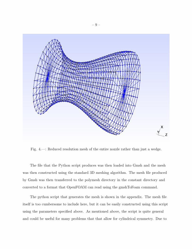
walls. A reduced resolution version of what the entire nozzle would like if the wedges were

rotated around the z axis is shown in Figure 4

– 7 –

Fig. 2.—: Lower resolution representation of the mesh produced by the custom Python

script and Gmsh for visualization. The mesh resolution shown here has been lowered by a

factor of 10.

– 8 –

Fig. 3.—: Zoomed in view of the actual mesh used for simulation at the wall near the outlet.

The resolution of the mesh increases as a function of radius to ensure that more complicated

interactions with the wall are captured correctly.

– 9 –

Fig. 4.—: Reduced resolution mesh of the entire nozzle rather than just a wedge.

The file that the Python script produces was then loaded into Gmsh and the mesh

was then constructed using the standard 3D meshing algorithm. The mesh file produced

by Gmsh was then transferred to the polymesh directory in the constant directory and

converted to a format that OpenFOAM can read using the gmshToFoam command.

The python script that generates the mesh is shown in the appendix. The mesh file

itself is too cumbersome to include here, but it can be easily constructed using this script

using the parameters specified above. As mentioned above, the script is quite general

and could be useful for many problems that that allow for cylindrical symmetry. Due to

– 10 –

computational time constraints, only one mesh was run.

Initially, an unstructured mesh of the entire 3D nozzle was tried rather than a simple

wedge, but ultimately failed. After a few time steps the CFL number became larger than 1

and the simulation crashed. This caused the movement towards the simpler wedge mesh,

which allowed for the construction of a structured mesh, and reduced computing costs.

Under the full 3D nozzle construction there were multiple issues with cell skewness and high

aspecect ratio cells that were flagged by the OpenFOAM command checkMesh as issues.

With the simpler wedge construction, there were much fewer issues the mesh.

4.2. Numerical Solver

The OpenFOAM numerical solver that was chosen is rhoCentralFoam. This solver

has the ability to handle supersonic compressible flows, which is necessary for handling

the conditions expected to present within the nozzle. This scheme is a density-based

compressible flow solver based on central-upwind schemes of (Kurganov and Tadmor

2000). The fluid parameters tracked throughout the simulation are temperature, velocity,

density and pressure. The parameter files for fvSchemes and fvSolution are shown in the

appendix.

Because this simulation is run under non-isothermal conditions, a thermophysicalProperties

file is required. The solver uses a ‘hePsiTherm’ thermoType keyword that constructs a

psiThermo thermodynamical model based on compressibility of the fluid for a system with

a fixed composition. A second keyword, pureMixture ensures that the simulation is run

without reactions and a perfect gas is assumed. The thermodynamic qualities of the fluid

are set such to approximate the fluid as air. The flow is assumed to be laminar, which is

set in the turbulenceProperties file.

– 11 –

4.3. Boundary and Initial Conditions

The boundary conditions for this problem were defined using the physical regions

defined the by Python script. The line that traces the axis of the simulation uses the empty

boundary condition and the two faces of the wedge use the wedge boundary condition for

all parameters, making the assumption of cylindrical symmetry. The outer wall of the

simulation uses a slip boundary condition for simplicity as the boundary layer at the wall

is not the focus of this simulation. The parameters that require boundary conditions are

velocity, pressure and temperature. The individual boundaries for the inlet and outlet for

each parameter are described below. The parameter files for each set of boundary conditions

are shown in the appendix. Because the wedge boundary condition was used at the two

faces, the boundary file within the polymesh directory also needed to be updated.

4.3.1. Pressure

The inlet boundary uses the totalpressure boundary which is useful for inlets where

the velocity is not known a priori. This condition sets the pressure equal to a constant for

outflow (a standard outflow boundary), but allows it to find its own value for inflow. The

outlet boundary uses the waveTransmissive boundary to avoid spurious wave reflections

off of the boundary and define the pressure difference across the nozzle. The choice of the

pressure difference, along with the cross sectional area of the nozzle, between the inlet and

the outlet is what sets the velocity and temperature distribution within the nozzle.

4.3.2. Velocity

The inlet and outlet both use a zeroGradient boundary condition. This allows the

velocity distribution to be extrapolated to the boundaries from the conditions within the

– 12 –

nozzle, which in the most part are governed by the difference in pressure accross the nozzle.

4.3.3. Temperature

The inlet boundary uses a fixedValue condition, fixed at a temperature of 298K (room

temperature). The outlet boundary uses a zeroGradient boundary condition under the

same premise as the velocity; the flow is allowed to evolve naturally under a fixed pressure

gradient.

4.4. Control

The time step for this simulation was chosen dynamically using the adjustTimeStep

keyword within the control file. This allows to simulation to increase the time step until the

Courant number reaches a specified limit. In this simulation, a maximum Courant number

of 0.5 was chosen to ensure stability. At most points during the simulation, the time step

is around 1 × 10−8 s. The simulation was run for 0.02 seconds and the parameters with

reported every 1× 10−4 seconds, yielding a total of 200 snapshots.

4.5. Sampling

A sample of the simulation was excised along the length of the nozzle slightly above

the symmetry axis. The first point in cartensian coordinates lies at (0.1 0.0 0.005) and the

final point lies at (0.1 0.0 1.995). The points were sampled in evenly spaced increments

along a straight line with 100 points. The ‘sampleDict’ file is shown in the appendix.

– 13 –

5. Results

5.1. Supersonic de Laval Nozzle

Here the results from the supersonic simulation are presented and discussed. Because

of high numerical costs, only one simulation is presented. This simulation took ∼ 4 days to

run on the Shared Computer Cluster. The solver used for this simulation is not currently

parallelized, but does have the potential to be.

5.1.1. Transient behavior

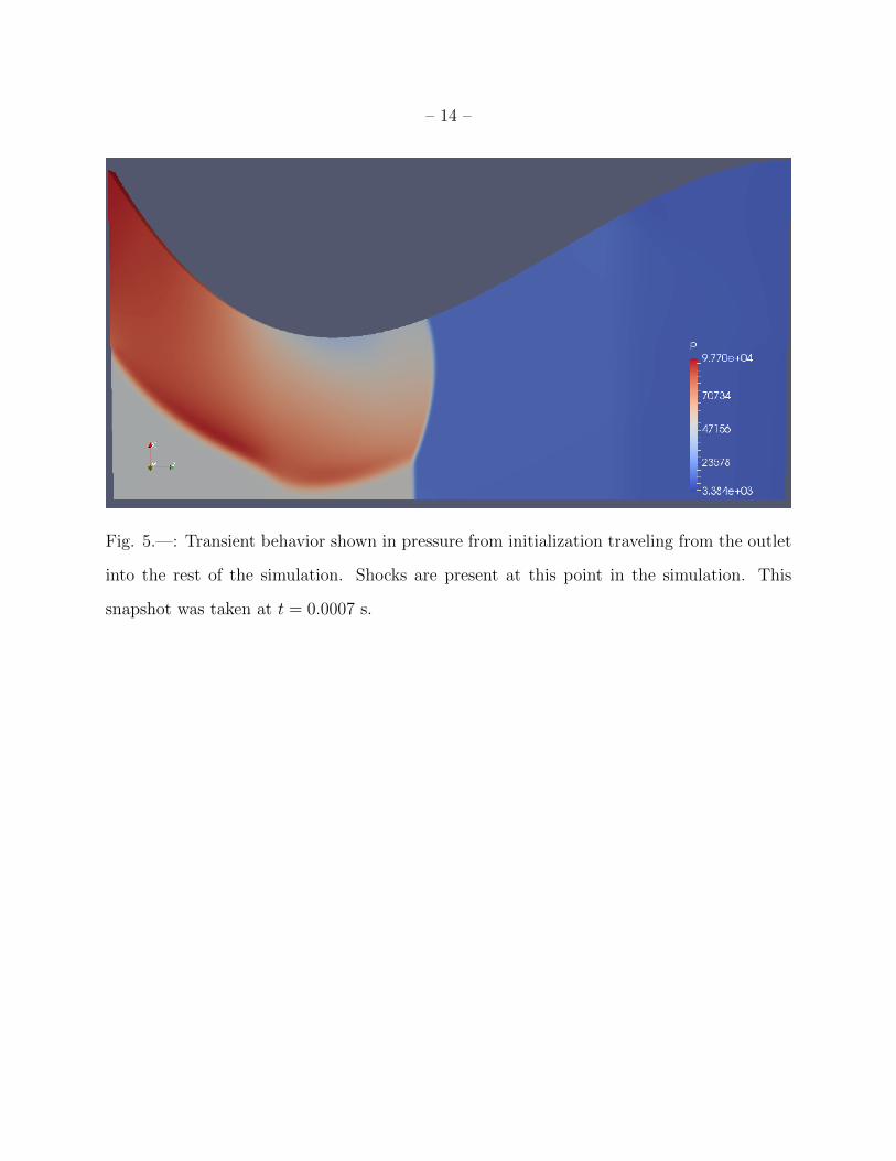
As the simulation begins, shocks propagate from the high pressure inlet region and

travel outward (see Figure 5). Waves reflect off of the outer walls. Due to symmetry, these

reflected waves interact with their complement waves near the center of the nozzle (see

Figure 6), providing a nice check that the wedge boundary conditions are working correctly.

Gradually the simulation begins to settle into a steady state flow, roughly around 0.01 s.

– 14 –

Fig. 5.—: Transient behavior shown in pressure from initialization traveling from the outlet

into the rest of the simulation. Shocks are present at this point in the simulation. This

snapshot was taken at t = 0.0007 s.

– 15 –

Fig. 6.—: Shocks crashing into each other along the symmetry axis. This snapshot is at

t = 0.00115 s. The shock front is still present at this time but is rapidly approaching the

outlet.

5.1.2. Flow structure

Once the transient behavior has subsided, clear patterns emerge. The flow smoothly

becomes supersonic roughly where the throat of the nozzle is at it’s narrowest point (Figure

7). Note that the line separating subsonic from supersonic flow is not quite straight,

likely showing the effects of adding viscosity to the fluid. Figures, 8, 9, and 10 show the

density, pressure, temperature and speed distributions across the nozzle once transients

have dissipated. All of these structures presented in these figures are reminiscent of the

theoretical structure predicted by the analytic inviscid case.

– 16 –

Fig. 7.—: Mach number once transients have dissapated. The green band shows where

the flow becomes supersonic, roughly where dAdz

= 0. Note that the curved nature of the

transition is not predicted by the analytic solution. Note that the Mach number contains all

components of the flow, which may be part of why the sonic point is curved.

– 17 –

Fig. 8.—: Pressure distribution across the nozzle in N/m2.

Fig. 9.—: Temperature distribution across the nozzle in K.

– 18 –

Fig. 10.—: Speed distribution across the nozzle in m/s. Note that the speed shown here

includes all components of the velocity.

Figure 11 shows the mach number in the final snapshot of the simulation measured

along the central axis once the flow has converged to steady state. Plotted alongside the

result is the analytic result for the Mach number of the inviscid de Laval nozzle with the

same geometry. Here the simulation does differ a bit from the analytic solution. The

addition of viscosity, and potentially numerical artefacts from the process of simulation,

have slowed down the supersonic flow, resulting in an exit Mach number of ∼ 2.5 rather

than the predicted ∼ 3.0. The flow also passes through the sonic point slightly further

down the nozzle than predicted by the analytic results.

– 19 –

0.0 0.5 1.0 1.5 2.0

z [m]

0.0

0.5

1.0

1.5

2.0

2.5

3.0

3.5

MachNumber

M= 1

SimulationAnalytic

Fig. 11.—: Comparison of the Mach number as a function of z between the simulation and

the analytic result for an inviscid de Laval nozzle. The sonic point is shown as dashed line.

The Mach number for the simulation was sampled along the z axis at a height of 0.1m above

the axis of symmetry.

A similar plot is shown for the temperature structure in Figure 12. For the subsonic

flow, the temperature structure closely follows the analytic solution. However, as the flow

becomes supersonic, a difference of ∼ 40K gradually develops over the length of the nozzle

with the simulation being hotter than the analytic solution. This is reasonable, as viscosity

only present in the simulation will transform some of the kinetic energy of the flow into

thermal energy. Finally, a comparison of pressure against the analytic case is shown in

Figure 13. Again, in the subsonic regime before the choke point there is good agreement

with the analytic case and as the flow becomes faster, larger deviations appear. Overall, the

predictions made by theory seems to be fairly well replicated by the simulation given that

the analytic solution is inviscid. The viscosity of the simulation presents itself by heating

and slowing down the supersonic flow.

– 20 –

0.0 0.5 1.0 1.5 2.0

z [m]

100

150

200

250

300

T[K

]

SimulationAnalytic

Fig. 12.—: Comparison between the simulation and the analytic solution for temperature as

a function of z. The temperature of the simulation is notably higher than the temperature

predicted by the analytic solution. This is likely due to the introduction of viscous forces.

0.0 0.5 1.0 1.5 2.0

z [m]

0

20000

40000

60000

80000

100000

p[N/m

2]

SimulationAnalytic

Fig. 13.—: Comparison between the simulation and the analytic solution for pressure as

a function of z. Again, a deviation is seen from the analytic as the velocity is accelerated

through the nozzle.

– 21 –

5.2. Convergence

When the simulation converges to steady state, the difference in tracked parameters

between one time step to another should become smaller. These differences between the

two steps are known as the residuals. If the residuals are plotted as a function of time one

can observe how quickly the simulation approaches steady state and when it has sufficiently

converged. Unfortunately, the majority of the residuals for the supersonic case were

overwritten as the simulation was interrupted several times throughout its run. However,

the residuals for Uz a subsonic case are shown in Figure 14.

– 22 –

Fig. 14.—: Uz residuals as a function of time for a subsonic case. Over time the residuals

decay to a roughly constant value, consistant with the simulation approaching residuals

resembling numerical error.

6. Conclusions

A de Laval nozzle was constructed uses a custom python script that generates structures

meshes of wedges of axisymmetric pipes. Using the rhoCentralFoam solver packed with

OpenFOAM, a steady state transonic solution was found. This solution was then compared

against the known analytic result and was found to be in relatively good agreement. The

– 23 –

deviations from the exact solution are likely due to the addition of viscosity which would

serve to slow and heat the flow as the kinetic energy is transferred into thermal energy,

which is what is observed in a line measurement taken along the axis of the simulation.

Future work for this project includes investigating how the results change with grid

resolution, because as it currently stands, the simulation takes a very long time to run.

Because of this, it is not clear if the simulation is in a state of mesh convergence. Expanding

the simulation to include the area behind the outlet would also be interesting, and would

potentially allow us to study the ‘shock diamonds’ that form behind this sort of nozzle.

The flexibility of the mesh generating code would make this fairly straightforward, although

more physical regions would need to be defined.

– 24 –

REFERENCES

Choudhuri, A. R. (1998). The physics of fluids and plasmas : an introduction for

astrophysicists.

Kurganov, A. and Tadmor, E. (2000). New high-resolution central schemes for nonlinear

conservation laws and convectiondiffusion equations. Journal of Computational

Physics, 160(1):241 – 282.

7. Appendix

Included in this section are the parameter files that were used to run the supersonic

de Laval nozzle in addition to the custom python script used to generate the structured

mesh for the grid. The actual grid file is not included as it is remarkably large. The files

are listed here in the order in which they are presented above.

This manuscript was prepared with the AAS LATEX macros v5.2.

import numpy as npimport matplotlib.pyplot as pltimport pdb

'''makewedge.py

PURPOSE: Script that writes instructions to create a wedge shape for the CFD openfoam project. For use with Gmsh

AUTHOR: Connor Robinson, Dec 6th, 2016'''

#Set up paths for savingpath = '/Users/Connor/Desktop/Coursework/CFD/project/'outfile = 'mesh_shape.txt'

#Define the shape of the nozzle in 1D#Set the number of cells along the cylinderlength = 400

#Set up cells between the center of the cylinder and the axis#Specify number of cellshnum = 200

#Specify the transfinite progressive scaling for those cellshprog = .97

#Define r as a function of Zzbase = np.arange(length)r = (45-zbase**2/(.08*length)**2 + zbase**3/(.186*length)**3)r = (r/np.max(r))[::-1] #Reverse r (Better nozzle shape, not necessary)

#Scale zbase back to something reasonable.zbase = zbase/(length/2)

#Define the fraction of a circle for the wedge to include (1/144 = 2.5 degrees)anglefrac = 1/144

#Actually go about generating the mesh, unlikely necessary to change anything below here.anglepoints = 3

phi = [-np.pi*anglefrac,np.pi*anglefrac]

x = np.array([r * np.cos(p) for p in phi]).flatten()

– 25 –

y = np.array([r * np.sin(p) for p in phi]).flatten()

z = np.hstack([zbase, zbase, zbase])x = np.hstack([x,np.zeros(length)])y = np.hstack([y,np.zeros(length)])

vlines = []

#Give a number to each pointpoints = np.arange(length*anglepoints)+1counter = 1

#Connect the lines along the flow axis, start at bottom and work around with increasing phifor angle in np.arange(anglepoints): for xval in np.arange(length-1): vlines.append([counter, xval+ angle*length+1, xval+angle*length+2]) counter = counter +1 hlines = []nvert = counter -1

#Connect the lines around the tube, start at bottom and work way up.for zval in np.arange(length)+1: for angle in np.arange(anglepoints): if (zval == length) and (angle == anglepoints -2): #hlines.append([counter, zval+angle*length, length*anglepoints]) hlines.append([counter, length*anglepoints, zval+angle*length]) else: if angle == 2 or angle == 0: hlines.append([counter, zval+angle*length, np.mod(zval+(angle+1)*length, length*anglepoints)]) if angle == 1: hlines.append([counter, np.mod(zval+(angle+1)*length, length*anglepoints), zval+angle*length]) counter = counter+1

nhorz = counter - 1 -nvert

#Now form the line loops, start at bottom and work around with increasing philoop = []loopcounter = 1

for zval in np.arange(length-1): for angle in np.arange(anglepoints): loop.append([loopcounter,\

– 26 –

vlines[zval+(angle*(length-1))][0], \ hlines[(zval+1)*anglepoints + angle][0], \ vlines[np.mod(zval + (angle+1)*(length-1), (anglepoints)*(length-1))][0], \ hlines[zval*anglepoints + angle][0]]) loopcounter = loopcounter +1

#Write out the lines and line loops to a text file.file = open(path+outfile, 'w')

#Write each set of pointsfile.write('// Points \n')

for p in np.arange(length*anglepoints): file.write('Point ('+str(np.int(p+1))+') = {'+str(x[p])+','+str(y[p])+','+str(z[p])+',1};\n')

#Write the vertical linesfile.write('// Verticle lines \n')for v in vlines: file.write('Line('+str(np.int(v[0]))+') = {'+str(np.int(v[1]))+','+str(np.int(v[2]))+'};\n')

#Write the horizontal linesfile.write('// Horizontal lines \n')for h in hlines: file.write('Line('+str(np.int(h[0]))+') = {'+str(np.int(h[1]))+','+str(np.int(h[2]))+'};\n')

#Write the line loopssurfacecounter = 1file.write('// Line loops \n')for i, L in enumerate(loop): if i != len(loop)-2: if np.mod(i+1, 3) == 0: file.write('Line Loop('+str(np.int(L[0]))+') = {'+str(np.int(L[1]))+','+str(np.int(L[2]))+','+str(np.int(-L[3]))+','+str(np.int(-L[4]))+'};\n') if np.mod(i+2, 3) == 0: file.write('Line Loop('+str(np.int(L[0]))+') = {'+str(np.int(L[1]))+','+str(-np.int(L[2]))+','+str(np.int(-L[3]))+','+str(np.int(L[4]))+'};\n') if np.mod(i+3, 3) == 0: file.write('Line Loop('+str(np.int(L[0]))+') = {'+str(np.int(L[1]))+','+str(np.int(L[2]))+','+str(np.int(-L[3]))+','+str(np.int(-L[4]))+'};\n') #Handle the final loop... else:

– 27 –

file.write('Line Loop('+str(np.int(L[0]))+') = {'+str(np.int(L[1]))+','+str(-np.int(L[2]))+','+str(np.int(-L[3]))+','+str(np.int(L[4]))+'};\n') file.write('Ruled Surface('+str(surfacecounter)+') = {'+str(surfacecounter)+'};\n') surfacecounter = surfacecounter +1

#Set up side1, side2, and the outer wall#Side1string =''file.write('Physical Surface("Left") = {')for val in np.arange(loop[-1][0])+1: if np.mod(val, 3) == 0: string = string+(np.str(np.int(val))+',')file.write(string[:-1]+'};\n')

#Side2string =''file.write('Physical Surface("Right") = {')for val in np.arange(loop[-1][0])+1: if np.mod(val+1, 3) == 0: string = string+(np.str(np.int(val))+',')file.write(string[:-1]+'};\n')

#outerwallstring =''file.write('Physical Surface("Outerwall") = {')for val in np.arange(loop[-1][0])+1: if np.mod(val+2, 3) == 0: string = string+(np.str(np.int(val))+',')file.write(string[:-1]+'};\n')

#Set up line loop and empty surface for axis:string = ''file.write('Physical Line("Axis") = {')for val in np.arange(length-1)+(length)*2-1: string = string+(np.str(np.int(val))+',')file.write(string[:-1]+'};\n')

#Form a volume for each cell in the center#Write the internal lineinteriorloopstart = surfacecounterfor val in np.arange(length): string = 'Line loop('+str(surfacecounter)+') = {' baseval = (val+length-1)*3 string = string + str(-int(baseval+3))+','+str(int(baseval+2))+','+str(-int(baseval+1))

– 28 –

file.write(string+'};\n') file.write('Ruled Surface('+str(surfacecounter)+') = {'+str(surfacecounter)+'};\n') surfacecounter = surfacecounter+1 file.write('Physical Surface("Input") = {'+str(interiorloopstart)+'};\n')file.write('Physical Surface("Output") = {'+str(surfacecounter-1)+'};\n')

volcounter = 1for val in (np.arange(length-1)): string = 'Surface loop('+str(volcounter)+') = {' string = string+(np.str(np.int(val*3+1))+',') string = string+(np.str(np.int(val*3+2))+',') string = string+(np.str(np.int(val*3+3))+',') string = string+(np.str(np.int(interiorloopstart+val))+',') string = string+(np.str(np.int(interiorloopstart+val+1))) file.write(string+'};\n') file.write('Volume('+str(volcounter)+') = {'+str(volcounter)+'};\n') volcounter = volcounter+1

#Set up the mesh structure for the horizontal lines

string = ''file.write('Transfinite Line {')for val in np.arange(nhorz): #if val != nhorz-1: if np.mod(val, 3) != 0: string = string+str(int(val+nvert+1))+','

file.write(string[:-1]+'} = '+str(hnum)+' Using Progression '+str(hprog)+';\n')

#Set up the mesh for the outer wallstring = ''file.write('Transfinite Line {')for val in np.arange(nhorz): #if val != nhorz-1: if np.mod(val, 3) == 0: string = string+str(int(val+nvert+1))+','

file.write(string[:-1])file.write('} = 1;\n')

#Set up the mesh structure for the vertical linesfile.write('Transfinite Line {')for val in np.arange(nvert): if val != nvert-1:

– 29 –

#if np.mod(val, 3) != 0 and val != nhorz-1: file.write(str(int(val+1))+',') if val == nvert-1: #if (np.mod(val, 3) != 0) and val == nhorz-1: file.write(str(int(val+1)))file.write('} = 1;\n')

file.write('Transfinite Surface "*";\n')file.write('Recombine Surface "*";\n')

file.write('Transfinite Volume "*";\n')

string = 'Physical Volume("internal") = {'

for val in np.arange(volcounter-1)+1: string = string+str(int(val))+',' file.write(string[:-1]+'};\n')

file.close()

– 30 –

/*--------------------------------*- C++ -*----------------------------------*\| ========= | || \\ / F ield | OpenFOAM: The Open Source CFD Toolbox || \\ / O peration | Version: 2.4.0 || \\ / A nd | Web: www.OpenFOAM.org || \\/ M anipulation | |\*---------------------------------------------------------------------------*/FoamFile{ version 2.0; format ascii; class dictionary; location "system"; object fvSchemes;}// * * * * * * * * * * * * * * * * * * * * * * * * * * * * * * * * * * * * * //

fluxScheme Kurganov;

ddtSchemes{ default Euler;}

gradSchemes{ default Gauss linear;}

divSchemes{ default none; div(tauMC) Gauss linear;}

laplacianSchemes{ default Gauss linear corrected;}

interpolationSchemes{ default linear; reconstruct(rho) vanLeer; reconstruct(U) vanLeerV; reconstruct(T) vanLeer;}

snGradSchemes{

– 31 –

default corrected;}

// ************************************************************************* //

– 32 –

/*--------------------------------*- C++ -*----------------------------------*\| ========= | || \\ / F ield | OpenFOAM: The Open Source CFD Toolbox || \\ / O peration | Version: 2.4.0 || \\ / A nd | Web: www.OpenFOAM.org || \\/ M anipulation | |\*---------------------------------------------------------------------------*/FoamFile{ version 2.0; format ascii; class dictionary; location "system"; object fvSolution;}// * * * * * * * * * * * * * * * * * * * * * * * * * * * * * * * * * * * * * //

solvers{ "(rho|rhoU|rhoE)" { solver diagonal; }

U { solver smoothSolver; smoother GaussSeidel; nSweeps 2; tolerance 1e-10; relTol 0; }

e { $U; tolerance 1e-10; relTol 0; }}

// ************************************************************************* //

– 33 –

/*--------------------------------*- C++ -*----------------------------------*\| ========= | || \\ / F ield | OpenFOAM: The Open Source CFD Toolbox || \\ / O peration | Version: 2.4.0 || \\ / A nd | Web: www.OpenFOAM.org || \\/ M anipulation | |\*---------------------------------------------------------------------------*/FoamFile{ version 2.0; format ascii; class dictionary; location "constant"; object thermophysicalProperties;}// * * * * * * * * * * * * * * * * * * * * * * * * * * * * * * * * * * * * * //

thermoType{ type hePsiThermo; mixture pureMixture; transport sutherland; thermo hConst; equationOfState perfectGas; specie specie; energy sensibleInternalEnergy;}

mixture{ specie { nMoles 1; molWeight 28.96; } thermodynamics { Cp 1004.5; Hf 0; } transport { As 1.458e-06; Ts 110.4; Pr 1; }}

// ************************************************************************* //

– 34 –

– 35 –

/*--------------------------------*- C++ -*----------------------------------*\| ========= | || \\ / F ield | OpenFOAM: The Open Source CFD Toolbox || \\ / O peration | Version: 2.4.0 || \\ / A nd | Web: www.OpenFOAM.org || \\/ M anipulation | |\*---------------------------------------------------------------------------*/FoamFile{ version 2.0; format ascii; class dictionary; location "constant"; object turbulenceProperties;}// * * * * * * * * * * * * * * * * * * * * * * * * * * * * * * * * * * * * * //

simulationType laminar;

// ************************************************************************* //

– 36 –

/*--------------------------------*- C++ -*----------------------------------*\| ========= | || \\ / F ield | OpenFOAM: The Open Source CFD Toolbox || \\ / O peration | Version: 2.4.0 || \\ / A nd | Web: www.OpenFOAM.org || \\/ M anipulation | |\*---------------------------------------------------------------------------*/FoamFile{ version 2.0; format ascii; class polyBoundaryMesh; location "constant/polyMesh"; object boundary;}// * * * * * * * * * * * * * * * * * * * * * * * * * * * * * * * * * * * * * //

5( Input { type patch; physicalType patch; nFaces 199; startFace 158204; } Output { type patch; physicalType patch; nFaces 199; startFace 158403; } Outerwall { type patch; physicalType patch; nFaces 399; startFace 158602; } Right { type wedge; physicalType wedge; nFaces 79401; startFace 159001; } Left { type wedge;

– 37 –

physicalType wedge; nFaces 79401; startFace 238402; })

// ************************************************************************* //

– 38 –

/*--------------------------------*- C++ -*----------------------------------*\| ========= | || \\ / F ield | OpenFOAM: The Open Source CFD Toolbox || \\ / O peration | Version: 2.4.0 || \\ / A nd | Web: www.OpenFOAM.org || \\/ M anipulation | |\*---------------------------------------------------------------------------*/FoamFile{ version 2.0; format ascii; class volScalarField; object p;}// * * * * * * * * * * * * * * * * * * * * * * * * * * * * * * * * * * * * * //

dimensions [1 -1 -2 0 0 0 0];

internalField uniform 15000;

boundaryField{

Output { type waveTransmissive; field p; phi phi; rho rho; psi thermo:psi; gamma 1.4; fieldInf 2533.33; lInf 1; value uniform 2533.33; }

Outerwall { type slip; }

Input { type totalPressure; U U; phi phi; rho none;

– 39 –

psi none; gamma 1.4; p0 uniform 101325; value uniform 101325;

}

Left {type wedge;} Right {type wedge;} Axis {type empty;}}

// ************************************************************************* //

– 40 –

/*--------------------------------*- C++ -*----------------------------------*\| ========= | || \\ / F ield | OpenFOAM: The Open Source CFD Toolbox || \\ / O peration | Version: 2.4.0 || \\ / A nd | Web: www.OpenFOAM.org || \\/ M anipulation | |\*---------------------------------------------------------------------------*/FoamFile{ version 2.0; format ascii; class volVectorField; object U;}// * * * * * * * * * * * * * * * * * * * * * * * * * * * * * * * * * * * * * //

dimensions [0 1 -1 0 0 0 0];

internalField uniform (5 0 0);

boundaryField{ Input { type zeroGradient; }

Output { type zeroGradient; }

Outerwall { type slip; }

Left {type wedge;} Right {type wedge;} Axis {type empty;}}

// ************************************************************************* //

– 41 –

/*--------------------------------*- C++ -*----------------------------------*\| ========= | || \\ / F ield | OpenFOAM: The Open Source CFD Toolbox || \\ / O peration | Version: 2.4.0 || \\ / A nd | Web: www.OpenFOAM.org || \\/ M anipulation | |\*---------------------------------------------------------------------------*/FoamFile{ version 2.0; format ascii; class volScalarField; object T;}// * * * * * * * * * * * * * * * * * * * * * * * * * * * * * * * * * * * * * //

dimensions [0 0 0 1 0 0 0];

internalField uniform 298.0;

boundaryField{ Input { type fixedValue; value uniform 298.0; }

Output { type zeroGradient; }

Outerwall { type slip; }

Left {type wedge;} Right {type wedge;} Axis {type empty;}}

// ************************************************************************* //

– 42 –

/*--------------------------------*- C++ -*----------------------------------*\| ========= | || \\ / F ield | OpenFOAM: The Open Source CFD Toolbox || \\ / O peration | Version: 2.4.0 || \\ / A nd | Web: www.OpenFOAM.org || \\/ M anipulation | |\*---------------------------------------------------------------------------*/FoamFile{ version 2.0; format ascii; class dictionary; location "system"; object controlDict;}// * * * * * * * * * * * * * * * * * * * * * * * * * * * * * * * * * * * * * //

application rhoCentralFoam;

startFrom latestTime;

startTime 0.0161;

stopAt endTime;

endTime 2e-02;

deltaT 1e-10;

writeControl adjustableRunTime;

writeInterval 1e-04;

cycleWrite 0;

writeFormat ascii;

writePrecision 15;

writeCompression off;

timeFormat general;

timePrecision 6;

adjustTimeStep yes;

maxCo 0.5;

maxDeltaT 1;

– 43 –

// ************************************************************************* //

– 44 –

/*--------------------------------*- C++ -*----------------------------------*\| ========= | || \\ / F ield | OpenFOAM: The Open Source CFD Toolbox || \\ / O peration | Version: 2.4.0 || \\ / A nd | Web: www.OpenFOAM.org || \\/ M anipulation | |\*---------------------------------------------------------------------------*/FoamFile{ version 2.0; format ascii; class dictionary; location "system"; object sampleDict;}// * * * * * * * * * * * * * * * * * * * * * * * * * * * * * * * * * * * * * //

interpolationScheme cellPoint;

setFormat raw;

sets( horizontalLine { type uniform; axis distance; start ( 0.1 0.0 0.005 ); end ( 0.1 0.0 1.995 ); nPoints 100; });

fields ( p U T);

// ************************************************************************* //

– 45 –