fmri preprocessing - wellcome trust centre for … · fmri preprocessing ... a continuous function...

fMRI

Preprocessing

Guillaume Flandin

Wellcome Trust Centre for Neuroimaging

University College London

SPM Course

Chicago, 22-23 Oct 2015

Normalisation

Statistical Parametric Map

Image time-series

Parameter estimates

General Linear Model Realignment Smoothing

Design matrix

Anatomical

reference

Spatial filter

Statistical

Inference RFT

p <0.05

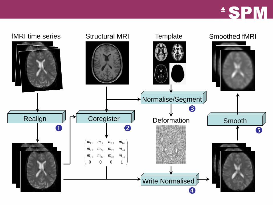
Realign

fMRI time series Structural MRI Template Smoothed fMRI

Deformation Smooth Coregister

Write Normalised

Normalise/Segment

1000

34333231

24232221

14131211

mmmm

mmmm

mmmm

Contents

Registration basics

Motion and realignment

Inter-modal coregistration

Spatial normalisation

Gaussian smoothing

Contents

Registration basics Voxel-to-world mapping

Transformation

Similarity measure

Optimisation

Interpolation




Gaussian smoothing

Representation of imaging data

Three dimensional images are made up of voxels.

Voxel intensities are stored on disk as lists of numbers.

Meta-information about the data:

– The image dimensions

• Allowing conversion from list to 3D array

– The “voxel-to-world mapping”

• Spatial transformation that maps from data coordinates (voxel column i,

row j, slice k) into a real-world position (x,y,z mm) in a coordinate

system e.g.:

– Scanner coordinates

– T&T/MNI coordinates

Image registration

Process of transforming different set of images into one

coordinate system.

Two key ingredients:

Transformation type:

Rigid

Affine

Non-linear

Similarity measure:

Mean-squared difference

Correlation coefficient

Mutual information

Within-subject

Between-subject

Within-modality

Between-modality

Optimisation

Automatic image registration is done by using an

optimisation algorithm.

Optimisation involves finding some “best” parameters

according to an “objective function”, which is either

minimised or maximised.

Value of parameter

Objective

function

Most probable solution

(global optimum)

Local optimum Local optimum

Reoriented

(1x1x3 mm

voxel size)

Resliced

(to 2 mm

cubic)

Reslicing / Interpolation

Applying the transformation parameters, and re-sampling the

data onto the same grid of voxels as the target image

– reslicing, interpolation, regridding, transformation, and writing

Nearest neighbour

– Take the value of the

closest voxel

Tri-linear

– Just a weighted average of

the neighbouring voxels

– f5 = f1 x2 + f2 x1

– f6 = f3 x2 + f4 x1

– f7 = f5 y2 + f6 y1

Simple Interpolation

B-spline Interpolation

B-splines are piecewise polynomials

A continuous function is represented by a

linear combination of basis functions

2D B-spline basis functions of

degrees 0, 1, 2 and 3

Nearest neighbour and

trilinear interpolation are the

same as B-spline

interpolation with degrees 0

and 1.

Contents

Registration basics




Gaussian smoothing

Motion correction

Head movement is a very large source

of variance in fMRI data.

Motion correction: realign a time-series

of images acquired from the same

subject.

Within-subject transformation: rigid-body (6 parameters)

Within-modality: least squares objective function

0 10 20 30 40 50 60 70 80 90 -0.4

-0.2

0

0.2

0.4

image

mm

translation

x translation y translation z translation

0 10 20 30 40 50 60 70 80 90 -0.2

0

0.2

0.4

0.6

image

degr

ees

rotation

pitch roll yaw

Residual Errors from aligned fMRI

Slices are not acquired simultaneously

– rapid movements not accounted for by rigid body model

Resampling can introduce interpolation errors

– especially tri-linear interpolation

Image artefacts may not move according to a rigid body

model

– image distortion

– image dropout

Functions of the estimated motion parameters can be

modelled as confounds in subsequent analyses

Movement by Distortion Interaction of fMRI

Subject disrupts B0 field, rendering it

inhomogeneous

Distortions in phase-encode

direction

Subject moves during EPI time

series

Distortions vary with subject

orientation

Shape varies (non-rigidly)

“Realign & Unwarp”: generative

model that combines a model of

geometric distortions and a model of

subject motion to correct images.

No correction Correction by covariation Correction by Unwarp No correction

Movement correction strategies

Contents

Registration basics




Gaussian smoothing

Inter-modal registration.

Match images from same subject

but different modalities:

anatomical localisation of

single subject activations

achieve more precise spatial

normalisation of functional

image using anatomical image.

Coregistration (intra-subject, inter-modal)

Coregistration maximises Mutual Information

Joint histogram sharpness correlates with image alignment.

Mutual information and related measures attempt to quantify how

well one image predicts the other.

Between-modality registration:

Seek to measure shared information in some sense.

Coregistration

L/R translation (mm)

-50 -40 -30 -20 -10 0 10 20 30 40 50

Norm

alise

d m

utu

al in

form

atio

n

1

1.02

1.04

1.06

1.08

1.1

1.12

Contents

Registration basics




Unified segmentation

Gaussian smoothing

Spatial Normalisation

Spatial Normalisation - Reasons

Inter-subject averaging

– Increase sensitivity with more subjects

• Fixed-effects analysis

– Extrapolate findings to the population as a whole

• Random-effects analysis

Make results from different studies comparable by

aligning them to standard space.

Standard spaces

The MNI template follows the convention of T&T, but doesn’t match the particular

brain (http://imaging.mrc-cbu.cam.ac.uk/imaging/MniTalairach)

Talairach Atlas MNI/ICBM AVG152 Template

http://imaging.mrc-cbu.cam.ac.uk/imaging/MniTalairach





Unified Segmentation

Normalising segmented tissue maps should be more robust and precise than using the original images.

Tissue segmentation benefits from spatially-aligned prior tissue probability maps.

Combining normalisation and segmentation in a unified model: – Gaussian mixture model

segmentation

– Intensity inhomogeneity (bias field) correction

– Warping (non-linear registration)

Tissue intensity distributions (T1-weighted MRI)

Mixture of Gaussians

Classification is based on a Mixture of Gaussians model,

which represents the intensity probability density by a

number of Gaussian distributions.

Image Intensity

Frequency

Non-Gaussian Intensity Distributions

Multiple Gaussians per tissue class allow non-Gaussian

intensity distributions to be modelled.

– E.g. accounting for partial volume effects

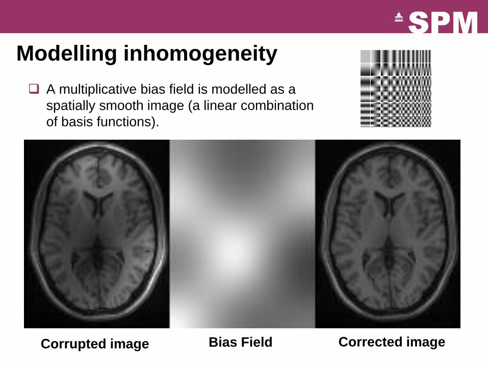
Modelling inhomogeneity

A multiplicative bias field is modelled as a

spatially smooth image (a linear combination

of basis functions).

Corrupted image Corrected image Bias Field

Tissue Probability Maps

Each TPM indicates the

prior probability for a

particular tissue at each

point in MNI space.

SPM12’s TPMs are

derived from the IXI

dataset initialised with the

ICBM 452 atlas and other

data.

Deforming the Tissue Probability Maps

Tissue probability

images are warped to

match the subject.

The inverse transform

warps to the TPMs.

Warps are constrained

to be reasonable by

penalising various

distortions

(regularisation).

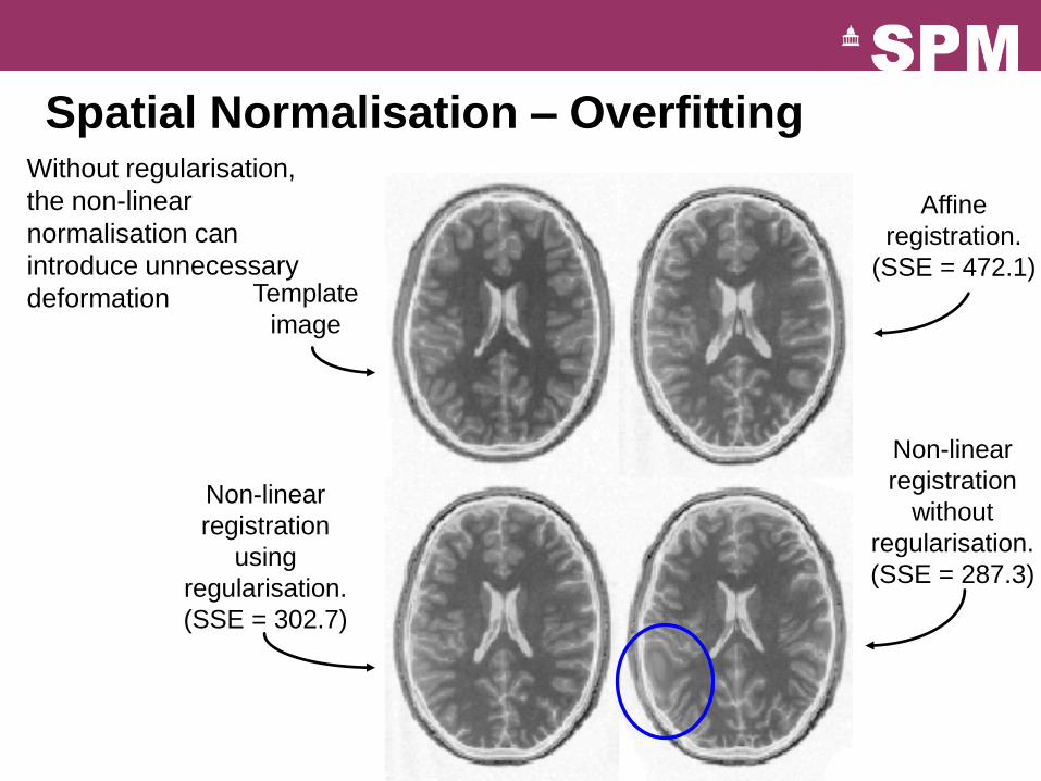
Template

image

Affine

registration.

(SSE = 472.1)

Non-linear

registration

without

regularisation.

(SSE = 287.3)

Non-linear

registration

using

regularisation.

(SSE = 302.7)

Without regularisation,

the non-linear

normalisation can

introduce unnecessary

deformation

Spatial Normalisation – Overfitting

Spatial Normalisation – Results

Non-linear registration Affine registration

Seek to match functionally homologous regions, but...

– No exact match between structure and function

– Different cortices can have different folding patterns

– Challenging high-dimensional optimisation, many local optima

Compromise

– Correct relatively large-scale variability (sizes of structures)

– Smooth over finer-scale residual differences

Spatial Normalisation – Limitations

Contents

Registration basics




Gaussian smoothing

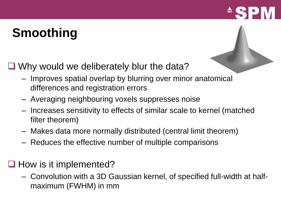
Smoothing

Why would we deliberately blur the data?

– Improves spatial overlap by blurring over minor anatomical

differences and registration errors

– Averaging neighbouring voxels suppresses noise

– Increases sensitivity to effects of similar scale to kernel (matched

filter theorem)

– Makes data more normally distributed (central limit theorem)

– Reduces the effective number of multiple comparisons

How is it implemented?

– Convolution with a 3D Gaussian kernel, of specified full-width at half-

maximum (FWHM) in mm

Effect of smoothing

3D Gaussian smoothing with FWHM: 0, 2, 4, 6, 8, 10, 12, 14, 16 mm isotropic

Realign



Write Normalised

Normalise/Segment

1000

34333231

24232221

14131211

mmmm

mmmm

mmmm

Normalise/Segment

Realign



Write Normalised

1000

34333231

24232221

14131211

mmmm

mmmm

mmmm

Realign

fMRI time series Template Smoothed fMRI

Deformation Smooth

Write Normalised

Normalise/Segment

References

Friston et al. Spatial registration and normalisation of images. Human Brain Mapping 3:165-189 (1995).

Collignon et al. Automated multi-modality image registration based on information theory. IPMI’95 pp 263-274 (1995).

Thévenaz et al. Interpolation revisited. IEEE Trans. Med. Imaging 19:739-758 (2000).

Andersson et al. Modeling geometric deformations in EPI time series. Neuroimage 13:903-919 (2001).

Ashburner & Friston. Unified Segmentation. NeuroImage 26:839-851 (2005).

Klein et al. Evaluation of 14 nonlinear deformation algorithms applied to human brain MRI registration. NeuroImage 46(3):786-802 (2009).

fmri preprocessing - wellcome trust centre for … · fmri preprocessing ... a continuous function...

Documents