Electronic copy available at: http://ssrn.com/abstract=1112629

A M ONTHLY VOLATILITY INDEX

FOR THEUS REAL ECONOMY

CECILIA FRALE ∗

cecilia.frale@uniroma2.it

DAVID VEREDAS †

david.veredas@ulb.ac.be

First Version 10/2007, This version: 02/2009

Abstract

We estimate the monthly volatility of the US economy from 1959 to 2008 by extending the factor

model of Stock and Watson (1991). The volatility of the factor, which we call VOLINX, has three ap-

plications. First, it measures the changes in uncertainty in the economy. VOLINX captures the decrease

in the volatility in the mid-80s (the so-called Great Moderation) as well as the different episodes of un-

certainty over the sample period. In the 70s and early 80s the stagflation and the two oil crises marked

the pace of the volatility whereas 09/11 is the most relevant shock after the moderation. Second, it helps

to understand the macroeconomic indicators that cause volatility. While industrial production is one

of the main drivers of the growth rate of the economy, its volatility is mainly affected by employment

and income. Last, the methodology we use permits us to estimate monthly GDP,which has conditional

volatility that is partly explained by VOLINX.

Keywords:Great Moderation, temporal disaggregation, volatility, dynamic factor models, Kalman filter.

J.E.L. Classification:C32, C51, E32, E37.

∗University of Tor Vergata, Rome, Italy.†ECARES, Universit́e Libre de Bruxelles, Brussels, Belgium.

We are grateful to Charles Bos, Gabriele Fiorentini, Domenico Giannone, Marc Hallin, Dieter Hess, Siem Jan Koopman, Massim-

iliano Marcellino, Tommaso Proietti, Kevin Shepard, Timo Terasvirta and Mark Watson for their remarks. We are also gratefulto

the participants of the ESEM 2008, the 5th Eurostat Colloquium on Tools for Business Cycle Analysis, Luxembourg (2008), the

conferences on Factor Structures for Panel and Multivariate Time Series Data, Maastricht (2008), and on Recent Developments in

Statistics and Econometrics. In Honour of Hirotugu Akaike, Kyoto (2008), and the seminar participants at ECARES, University Tor

Vergata and Aarhaus Business School. Routines are coded in Ox 3.3 by Doornik (2001) and provide an extension of the programs

realized by Tommaso Proietti for the Eurostat project on the Monthly GDP estimation. The second author gratefully acknowledges

financial support from the Belgian National Bank and the IAP P6/07 contract, from the IAP programme (Belgian Scientific Policy),

’Economic policy and finance in the global economy’. David Veredas is also member of ECORE, the recently created association

between CORE and ECARES. Any remaining errors and inaccuracies are ours.

Electronic copy available at: http://ssrn.com/abstract=1112629

1 Introduction

Timely information, say monthly, on the state of the economyis of paramount importance for economic

policy decision making. This information is typically summarized by the growth rate of the economy -

measured by synthetic indexes or observed indicators- and its volatility. Given a set of macroeconomic

indicators sampled from January 1959 to June 2008, we extendthe factor model of Stock and Watson

(1991) and we estimate a monthly index for the volatility of the US economy, which we call by VOLINX.

This index helps us to, among others, better understand the time varying uncertainty of the US economy,

possible structural changes (such as the Great Moderation), and determine the macroeconomic indicators

that create uncertainty in the economy.

Additionally, the model includes quarterly GDP, generallyconsidered the major indicator of the state

of the economy, as an additional source of information to themonthly indicators. The econometric model

we rely on (state space models) and its treatment of missing of observations allows us to obtain monthly

GDP estimates -similarly to Mariano and Murasawa (2003). GDP presents time-varying volatility that is

partially captured by VOLINX.

There is an increasing number of articles that look at using coincident indexes and high frequency

measures of the state of the economy to monitor its evolution. We identify two main approaches: studies

that use monthly information to extract the factors drivingthe economy, and studies that disaggregate

quarterly GDP. The first group of works goes back to the seminal paper of Stock and Watson (1991)

(S&W henceforth). They develop a factor model using a reduced set of well chosen indicators that are

believed to contain the most relevant information about thestate of the economy. More recently, Stock and

Watson (2002a) opt for a large scale dynamic factor model, inthe spirit of Forniet al (2000). By working

with monthly observations, this approach does not considerGDP. This issue motivates the second strand

of the literature. Chow and Lin (1971) first showed how monthly GDP series could be constructed from

regression estimates using GDP-related monthly indicators. Several authors improved on this idea by using

different multivariate disaggregation methods (see Harvey and Chung, 2000, Moauro and Savio, 2005 and

Proietti and Moauro, 2006). Evans (2005) presents an innovative model for estimating daily GDP. Finally,

Mariano and Murasawa (2003) (M&M henceforth) combine the two approaches - disaggregation and the

use of factors - casting S&W in a linear state space model defined at monthly frequency and including the

quarterly GDP.

The literature mentioned above ignores the stylized evidence which shows that most of the US macroe-

conomic indicators show time varying volatility over the last 30 years. This has received special attention

since the significant drop in uncertainty in the mid-80s, theso-called Great Moderation. As documented

by Stock and Watson (2002b), the majority of the 168 US economic variables that they analyze experience

a decline in volatility, characterized by a break in the fluctuations in the mid-80s. Top panel of Table 1

is evidence of this. It shows the sample standard deviationsof the log growth rate of quarterly GDP and

2

monthly employment, sales, industrial production and personal income, all in logs, from January 1959 to

June 2008.1. The change in the volatility pattern is clear. The Great Moderation led to a significant de-

crease in growth fluctuations. For instance, the sample standard deviation of quarterly GDP prior to 1985

was 10.70 while it dropped to 4.94 for the period 1985-2008, roughly half the previous value. Many au-

thors have argued that this is due to a change in the dynamic pattern of the economy, which model wise

is reflected in a change in the parameters of the conditional mean. In the context of factor models, this

means, for instance, a change in the factor loadings. However, as it is shown in Section 2, time varying

factor loadings and time varying volatility are observationally equivalent.

On the basis of this, Stock and Watson (2002b) estimate univariate dynamic conditional variances for

the 168 series using Stochastic Volatility (SV henceforth)models. Figure 1 shows the five above mentioned

observed indicators. Visual inspection reveals that growth rates show conditional heteroskedastic. The

bottom panel of Table 1 shows the GARCH(1,1) estimates for each indicator. All the estimated volatilities

present persistence, except maybe for employment, as measured by the GARCH term, and they are all

affected by shocks, specially employment, measured by the ARCH term.

Stock and Watson (2007) further develop the SV model for inflation. Based on the fact that an

ARIMA(0,1,1) model can be expressed as a local level model (i.e. a random walk plus noise), they separate

volatility into permanent and transitory components, and consider time-varying moving average parame-

ters. This flexibility allows them to explain a variety of recent univariate inflation forecasting puzzles. Other

researchers have followed similar approach, analyzing thefluctuations of the US economy with particular

focus on inflation and monetary policy. By using different models and theoretical approaches, they all find

evidence of a decrease in volatility for inflation, which reflects a reduction in the volatility of durable goods

production (McConnell and Perez Quiros, 2000), a change of monetary regime (Cecchetti et al., 2005, and

Primiceri, 2005), a change in government policy maker models (Cogley and Sargent, 2005) or a change in

policy rule coefficients (Sims and Zha, 2005).

In this paper we extend S&W in two directions that allow us to estimate monthly GDP and VOLINX.

We estimate the monthly GDP by disaggregating the quarterlyvalue using the technique for state space

models developed by Harvey (1989). In brief, this techniqueconsists of augmenting the state vector to

include monthly GDP as a latent process that can be estimatedwith the Kalman filter. A similar approach

has been used by Mariano and Murasawa (2003, 2004), Camacho and Perez-Quiros (2008) and Frale et al.

(2008).

To estimate VOLINX, we rely on a new type of GARCH model. It differs from the traditional version

by four aspects. First, it is a conditional volatility modelfor unobserved components and thus the errors

1These are the same indicators used by S&W and M&M, among others. Employment is defined as employees on non agricultural

payrolls (thousand, SA). Industrial Production is defined as an index of industrial production (2002=100,SA). Sales ismeasured by

manufacturing and trade sales (millions of chained (2000) dollars,SA). Income is defined as personal income less transfer payments

(billions of dollars, SA,AR). And finally, GDP stands for real GDP (billions of chained (2000) dollars, SA, AR). SA standsfor

seasonally adjusted and AR for annual growth rates. All datais downloadable from the NBER web site.

3

are also unobserved, as pointed out by Harvey, Ruiz and Sentana (1991). Second, similarly to Engle and

Rangel (2008), we adopt a multiplicative component model, where one component is slowly moving and

captures the permanent changes in volatility, and another component captures the short run dynamics of

macroeconomic fluctuations. Third, we replace the past square error by a linear combination of the past

standardized forecasting errors of the macroeconomic indicators. The forecasting errors can be seen as

the non-anticipated information, or the surprise. The weights attached to each past surprise are estimated

endogenously and allow us to determine which indicators most explain the volatility of the economy. Last,

VOLINX is the common volatility for all the indicators up to an idiosyncratic scale, which also allows us

to study the contemporaneous causality between the volatility of the factor and the indicators.

Our results show that the US economy suffered regular episodes of uncertainty prior to the Great Mod-

eration, for instance during the stagflation and the oil crisis. After the mid-80s, the volatility decreased

substantially. During the Clinton administration, the economy had a long period of steady growth without

significant uncertainty. Only two peaks show up after the Great Moderation. The first is in early 90s. This

is probably due to the invasion of Kuwait by Irak and the first Gulf war. The second is 09/11 and the

subsequent months, though the sudden increase in the uncertainty disappeared as quickly as it appeared.

Another usefulness of VOLINX is that it helps us to understand the determinants of uncertainty in the

US economy. As previously mentioned, we use the same set of macroeconomic indicators as in S&W

and M&M. They are also among the most important indicators used by the NBER dating committee. By

constraining ourselves to this set of indicators, we can investigate if the variables that are thought to be the

main drivers of the economy are also the main drivers of volatility. The answer is no. While we find that,

consistent with the literature, industrial production is the most important determinant for the level of the

US economy, employment and income are the most important determinants of the volatility, with industrial

production taking a backseat.

The structure of the paper is as follows. Section 2 presents the model and the theoretical properties

entailed by VOLINX. Section 3 briefly discusses estimation issues, including the specification of the model

in its space state form and the disaggregation of GDP. Section 4 shows the results and the analysis of the

estimated factor and VOLINX according the political and economic events over the sample, as well as the

NBER turning points. Section 5 concludes.

2 The model

Let yt, for t = 1, ..., T , denote anN × 1 vector of macroeconomic indicators, in logarithms, which

we assume to be integrated of order one, so that∆yi,t, i = 1, . . . , N , are the growth rates that have a

stationary and invertible representation. This vector contains both the monthly macro indicators and the

quarterly GDP.2 Following S&W,yt is expressed as a linear combination, withN×1 loadingstheta ∈ R,

2For the sake of clarity, we relegate the technical exposition of the disaggregation of quarterly GDP to Section 3.

4

of a factor (denoted byft) andN idiosyncratic components (gathered in theN × 1 vectorµt) specific for

each series:

yt = θft + µt,

which can also be written as

∆yt = θ∆ft + ∆µt. (1)

The factor follows an autoregressive difference process oforder one:

(1 − φL)∆ft = εt, (2)

where0 ≤ φ < 1 and the idiosyncratic components follow an AR difference process of order one with

drift:

D(L)∆µt = δ + ηt, (3)

whereδ ∈ RN is aN × 1 vector of intercepts andD(L) is a diagonal polynomial matrix:

D(L) = diag [(1 − d1L), (1 − d2L), . . . , (1 − dNL)] (4)

such that0 ≤ di < 1 for i = 1, . . . , N and the roots of|D(s)| = 0 are outside the unit circle. If the

disturbancesεt andηt are Gaussian, mutually uncorrelated at all leads and lags, the variance ofεt is 1, and

the idiosyncratic disturbances have constant variances, this model boils down to S&W, which we denote as

theS&W model.3 We propose a heteroskedastic framework that assumes a common time-varying volatility.

In order the understand the nature of the forthcoming equations, let us examine more carefully equation

(1). Taking expectation conditional to past information (denoted byIt−1) for theith indicator:

E[∆yi,t|It−1] = E[θi∆ft|It−1] + E[∆µi,t|It−1].

That is, the expected growth rate equals the expected growthrate of the factor (weighted by the factor

loading) plus theith idiosyncratic component. This additive decomposition is appropriate as it can be seen

as a location shift of the density for each economic indicator, with respect to the density of the factor. Shifts

in variances are, by contrast, more naturally understood asscale shifts, which lead to multiplicative forms.

Hence we assume that the conditional variance of the economic indicator equals:

V [∆yi,t|It−1] = V [∆ft|It−1]γi, (5)

whereγi > 0 is an idiosyncratic scale.4 In order to obtain (5) we assume:

εt|It−1 ∼ N (0, ht) and

ηt|It−1 ∼ N (0, ht diag(λ21, . . . , λ

2N )

︸ ︷︷ ︸

Λ

),

3Fixed variance and equal to 1 forηt is needed for identification, which is reached by concentrating it out of the log-likelihood

function.4This is not of course the only way to produce shifts in variances. Additive or both additive and multiplicative are also possible

(e.g. Diebold and Nerlove, 1989, and Sentana and Fiorentini, 2001).

5

which can be re-written as

εt

ηt

∣∣∣∣∣∣

It−1 ∼ N

0

0

, ht

1 0

0 Λ

. (6)

whereλi ∈ R for i = 1, . . . , N . Disturbances have variances equal to a shape matrix times the conditional

volatility ht that we call VOLINX. These assumptions imply a conditional variance of theith economic

indicator

V [4yi,t|It−1] = θ2i V [4ft|It−1] + V [4µi,t|It−1]

= θ2i ht + λ2iht = (θ2i + λ2

i )ht.

Hence, in (5),γi = θ2i + λ2i . More compactly:

V [4yt|It−1] = (θθ′ + Λ)ht. (7)

There are several possibilities for the specification of VOLINX. In light of the empirical evidence

presented in the introduction, one may think of a variance mechanism that considers two regimes, prior

and after the beginning of the Great Moderation, in line withStock and Watson (2002b) and the top panel

of Table 1:

ht = ω1I[1] + ω2I[2], (8)

whereω1 > 0, ω2 > 0, andI[1] (I[2] respectively) is an indicator function that takes value1 for t prior

(posterior respectively) to the Great Moderation.5 This is the second model we estimate and that we denote

Two regimesmodel.

This model does not capture the conditional heteroskedasticity found in the data and a GARCH-type

model seems more appropriate. However, when working with unobserved components, the residuals are

no longer equal to the difference between the observation and the prediction but, rather, between the un-

observed and its prediction. Harvey, Ruiz and Sentana (1991) introduce a GARCH model for unobserved

components defined in a state space framework:

ht = ω + βht−1 + αψ2t−1, (9)

whereω > 0, 0 ≤ β < 1, 0 ≤ α < 1 andβ + α < 1. The second component in the right hand side

is standard in the GARCH literature and captures the persistence while the third component isψ2t−1 =

E[ε2t−1|It−2] = V [εt−1|It−2] + E[εt−1|It−2]2, whereV [εt−1|It−2] andE[εt−1|It−2] are provided by

the Kalman filter. Although this method is rather appealing from an econometric point of view, it lacks

mechanisms to allow changes in the regime of the volatility.It also lacks an economic interpretation, in

the sense thatht should be caused, in some sense, by the past fluctuations of the indicators, instead of past

fluctuations of the factor.5The choice of the breaking date is discussed later.

6

In order to allow changes in the regime of the volatility and establish the link between past fluctuations

of the indicators andht, we consider a multiplicative component model, in the same spirit as Engle et. al

(2005):

ht = τtgt, (10)

whereτt characterizes the slowly moving variations in VOLINX, associated with common permanent

effects (such as the Great Moderation) andgt describes the short-run dynamics, associated with common

transitory effects. In a similar context to ours, Engle and Rangel (2008) propose a spline forτt. We, instead,

opt for a Fourier Series (in exponential) of order three:

τt = exp

ρ0 +

3∑

j=1

ρsj sin

(

2πjt

T

)

+ ρcj cos

(

2πjt

T

)

. (11)

whereρ0 ∈ R, ρsj ∈ R andρc

j ∈ R for j = 1, 2, 3. Since there is nothing random in this expression

E[τt] = E[τt|It−1] = τt. On the other hand, transitory effects are captured by the past expected short-run

volatility:

gt = (1 − β) + βgt−1 + α

N∑

i=1

ωiνi,t−1, (12)

where0 ≤ β < 1, α ≥ 0, ωi ≥ 0, and∑N

i=1 ωi = 1. The last term in the right hand side accounts

for shocks and is expressed as a linear combination of past forecasting errors of the indicators, which

can be seen as the non-anticipated information or surprise.Following the literature of macroeconomic

news announcements and their effect on financial markets, weassume that the uncertainty of the economy

increases when the growth rates of the main economic indicators vary more than expected. In other words,

it is the forecasting error what causes the uncertainty to increase, rather than the growth rate itself. The

standardized surprise for theith economic indicator is

νi,t−1 =4yi,t−1 − E[4yi,t−1|It−2]

√

V [4yi,t−1|It−2]

and whereE[4yi,t−1|It−2] andV [4yi,t−1|It−2] are provided by the Kalman filter. The weightsωi are

estimated and, sinceνi,t are standardized, they have a clear economic interpretation: we can infer which

are the indicators that explain the most the common volatility. The second term in the right hand side

of (12) is the traditional GARCH part of the model that captures the volatility clustering. Note that the

parameter constraints do not include the conditionβ +α < 1. As it will become clear below, this model is

less restrictive than a standard GARCH model in terms of existence of unconditional variance and kurtosis.

Last, the first term in the right hand side of the model is the intercept, specified such that the unconditional

expectation of the short-run volatility is one:

E[gt] = (1 − β) + βE[gt−1] + αN∑

i=1

ωiE[νi,t−1]

⇒ (1 − β)E[gt] = (1 − β) ⇒ E[gt] = 1,

7

so that the unconditional variance isE[ht] = τt, the smooth long-run component, similarly to Engle

and Rangel (2008). This model has the advantage that there isno need to assume breaking dates for the

changes of regime in the volatility. Take, for instance, theGreat Moderation. The literature on the Great

Moderation features extensive debates as to the date when itactually began, circa 1984. Stock and Watson

(2002b) attempt to date the Great Moderation using different methods. They find a breaking date for most

of the components series of GDP in February 1983 with a 67% confidence interval from April 1982 to

March 1985. With model (10) there is no need to specify a breaking date.

In the sequel of this Section we study the properties of the model. First, note that the disturbances can

be written as:

εt = h1/2t zt andηt = h

1/2t Λ1/2zt,

wherezt ∼ NID(0, 1) andzt ∼ NID(0, IN ) andIN isN size identity matrix. The first four uncondi-

tional moments of the disturbances are:

E[εt] = 0 and E[ηt] = 0

E[ε2t ] = τt and E[η2t ] = τtΛ

E[ε3t ] = 0 and E[η3t ] = 0

E[ε4t ] = 3κt and E[η4t ] = 3κtΛ

2.

Note that the even moments are not constant, since they depend on time, and whereκt = E[h2t ] is shown

in the following Proposition.

Proposition 1 Model (10) with (11) and (12) has unconditional second moment

κt = E[h2t ] = τ2

t κ̃

where

κ̃ =1 − β2 + α2

(∑N

i=1 ω2i +

∑

j,k,j 6=k cj,k

)

1 − β2

and

cj,k = 2ωjωkθjθk

(d2

j + λ2j

)1/2h

1/2t (d2

k + λ2k)

1/2h

1/2t

.

Two remarks on the result in Proposition 1. Fist, unlike in the traditional GARCH model, it is not

clear whether the unconditional distribution of the disturbances shows excess kurtosis. Nevertheless, it is

interesting to note that̃κ > 1 (unlessα = 0), meaning that, ifτt ≥ 1, εt shows excess kurtosis. Second, the

condition for existence of kurtosis is0 ≤ β < 1, a much weaker condition than in a standard GARCH(1,1).

The following Proposition shows the first four unconditional moments of the economic indicators.

8

Proposition 2 If yt follows the model described in (1)-(3), (6) and (10), the first four unconditional mo-

ments are

E[4yt] = D̃−1δ,

V [4yt] = τt

(

θθ′ 1

1 − φ2+ Λ̃

)

,

E[4y3t ] = 0 and

E[4y4t ] = 3κt

[1 + φ2

(1 − φ2)(1 − φ4)ΣΣ′ + Φ

]

+ 4τt

1 − φ2Σ(

B + D̃−2δ2)

.

Where

D̃ = diag(1 − d1, . . . , 1 − dN ),

Λ̃ = diag

(λ2

1

1 − d21

, . . . ,λ2

N

1 − d2N

)

,

Σ = ΛΛ′

Φ = diag

(

λ41

1 + d21

(1 − d21)(1 − d4

1), . . . , λ4

N

1 + d2N

(1 − d2N )(1 − d4

N )

)

and

B = diag

(λ2

1τt1 − d2

1

, . . . ,λ2

Nτt1 − d2

N

)

.

The conditional mean of the economic indicators (1) can be extended in several directions. The first

is by introducing lagged values of the factor. It may be the case that some of the economic indicators are

lagging the economy. A second extension is the inclusion of aset of exogenous regressors, denoted byxt,

that are used for calendar effects and intervention variables. Then (1) becomes

∆yt = θ1∆ft + θ2∆ft−1 + ∆µt + xtβ. (13)

The inclusion of these two terms affects the moments computed above but this is, however, a matter of

algebra.

Last, it is worth discussing the main difference of our paperto handle time varying volatility and

previous articles on the Great Moderation. Most of the recent studies propose models with parameter

instability, which can be found either in the parameters of the conditional mean, the variance-covariance

function itself, or both. Stock and Watson (2007) and Cecchetti et al. (2005) propose a simple univariate

unobserved component with stochastic volatility. The reduced form of this model is a moving average

with time varying moving average parameter that depends on the stochastic volatility. Cogley and Sargent

(2005) and Primiceri (2005) opt for a more complicated model. They propose a VAR model with drifting

parameters and stochastic volatility models. Sims and Zha (2005) propose a regime switching model where

the regimes are allowed in the parameters of the conditionalmean and the variances.

In our setting, however, parameter instability in the conditional mean and time varying volatility are

observationally equivalent. This is shown in the followingexample, taken from Engle et al. (1990), and

9

adapted to our notation. Let (1) but with time varying factorloadings:

4yt = θt4ft + 4µt.

Time varying factor loadings can be modelled in two different ways. Assume first thatθt = θh1/2t and that

the variance of the factor is constant:V [4ft] = 1. The variance of the idiosyncratic components is also

assumed to be constant:V [4µt|It−1] = Λ. Then, the conditional variance of the economic indicatorsis

V [4yt|It−1] = (θtθ′t + Λ) = htθθ′ + Λ.

Assume now that the factor loadings are constant,θt = θ, but that the variance of the factor is time varying:

V [4ft|It−1] = ht. Then, the conditional variance of the economic indicatorsis

V [4yt|It−1] = htθθ′ + Λ.

In both cases we obtain the same expression forV [4yt|It−1]. These two specifications are therefore obser-

vationally equivalent, meaning that, in our setting, the Great Moderation can be explained with either time

varying factor loadings or with time varying volatility. Weprefer the later since changes in volatility are, in

some sense, a data-driven phenomena while changes in factorloadings are a model-driven characterization.

3 Estimation

We show how to cast the model in a state space form that is suitable for applying the Kalman filter.6 For

the ease of exposition, we first consider the case where all series inyt are observed in the same frequency,

presenting the state space of each component separately, first for the factor followed by the idiosyncratic

components, and finally we put it all together to get the complete form. At the end of the Section we show

how to extend the state space representation to the temporaldisaggregation constraints.

Equation (1) can be written as∆ft = gf,t wheregf,t = φgf,t−1 + εt. Hence the state space represen-

tation of the model for the factor is

ft = efαf,t

αf,t = Tfαf,t−1 + e∗fεt,

where

ef = (1, 0), αf,t =

ft

gf,t

, Tf =

1 φ

0 φ

ande∗f =

1

1

.

A similar representation holds for each individualµi,t, with φ replaced bydi and introducing theith

interceptδi:

µi,t = eiαi,t

αi,t = Tiαi,t−1 + ci + e∗i ηi,t,

6The main lines of this section follow Frale et al. (2008).

10

where

ei = (1, 0), αi,t =

µi,t

gi,t

, Ti =

1 di

0 di

, ci =

δi

δi

ande∗i =

1

1

.

Combining these state space representations we obtain the state space form of the model:

yt = Zαt

αt = Tαt−1 + Hεt,

whereαt = [α′f,t,α

′1,t, . . . ,α

′N,t]

′ is a2 + 2N state vector,

Z =

θ1 0 e′f 0 . . . 0

θ2 0 0 e′1 . . . 0...

......

θN 0 0 0 . . . e′N

is aN × (2 + 2N) matrix,T = diag(Tf ,T1, . . . ,TN ) is a(2 + 2N) × (2 + 2N) block diagonal matrix,

H = diag(e∗f , e∗1, . . . , e

∗N ) is a (2 + 2N) × (1 + N) matrix, andεt = (εt,ηt) is a 1 + N vector of

disturbances with conditional distribution (6).

To deal with mixed frequency we follow Harvey (1989) operating a suitable augmentation of the state

vector. Let us partition the set of indicators,yt, into two groups,yt = (y′1,t, y

′2,t)

′, wherey1,t contains the

economic indicators observed at monthly frequency whiley′2,t is GDP observed only every three months.

Let y∗2,t be the (partially) unobserved monthly GDP. Since GDP is a flowrandom variable,

y2,τ =2∑

i=0

y∗2,3τ−i, τ = 1, 2, . . . , [T/3].

That is, the observed quarterly GPD is the sum of the unobserved current and two lagged monthly values.

Then, defineyc2,t = ψty

c2,t−1 + y∗2,t, whereψt is the cumulator variable, defined by:

ψt =

0 t = 3(τ − 1) + 1, τ = 1, . . . , [T/3]

1 otherwise.

The cumulator is equal to the observed aggregated series at timest = 3τ , and otherwise it contains the

partial cumulative monthly unobserved value. The final state space form of the model is

y∗t = Z∗α∗

t

α∗t = T∗α∗

t−1 + H∗εt,

wherey∗t = (y1,t y

c2,t), α∗

t = [α′f,t,α

′1,t, . . . ,α

′N,t, y

c2,t]

′ is a2 + 2N + 1 state vector,

Z∗ =

Z1 0

0 1

andT∗ =

T 0

Z2T ψt

11

are a(N + 1) × (2 + 2N + 1) matrices withZ2 the1 × (2 + 2N) block of the measurement matrixZ

corresponding to the GDP such thatZ = (Z′1 Z′

2)′. If for instance, GDP is theNth economic indicator,

Z2 = (θN 0 0 0 . . . e′N ). Last,

H∗ =

I2+2N

Z2

H

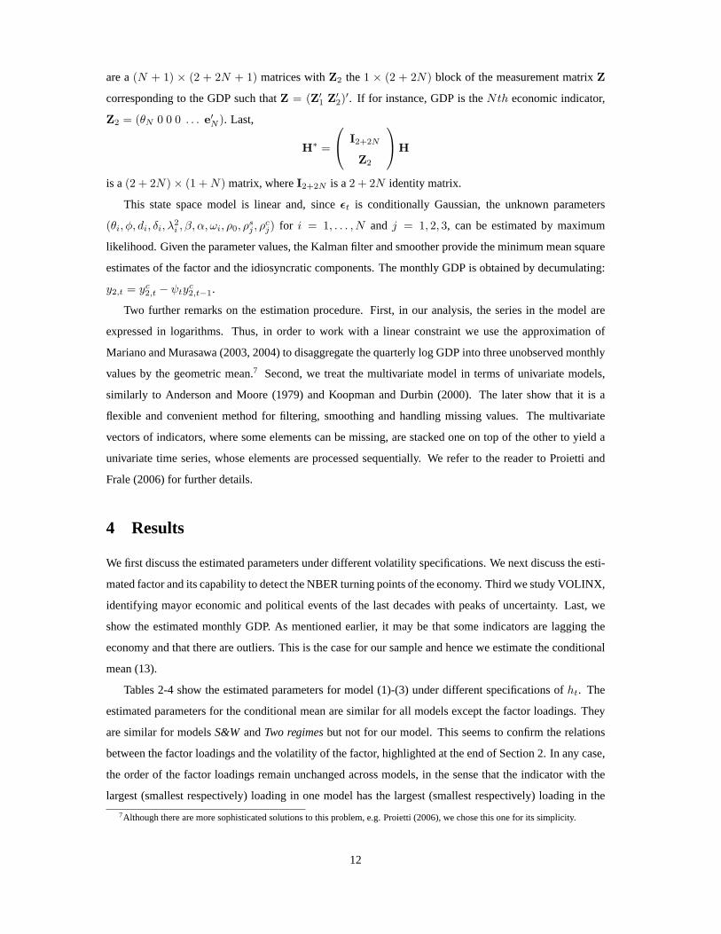
is a(2 + 2N) × (1 +N) matrix, whereI2+2N is a2 + 2N identity matrix.

This state space model is linear and, sinceεt is conditionally Gaussian, the unknown parameters

(θi, φ, di, δi, λ2i , β, α, ωi, ρ0, ρ

sj , ρ

cj) for i = 1, . . . , N and j = 1, 2, 3, can be estimated by maximum

likelihood. Given the parameter values, the Kalman filter and smoother provide the minimum mean square

estimates of the factor and the idiosyncratic components. The monthly GDP is obtained by decumulating:

y2,t = yc2,t − ψty

c2,t−1.

Two further remarks on the estimation procedure. First, in our analysis, the series in the model are

expressed in logarithms. Thus, in order to work with a linearconstraint we use the approximation of

Mariano and Murasawa (2003, 2004) to disaggregate the quarterly log GDP into three unobserved monthly

values by the geometric mean.7 Second, we treat the multivariate model in terms of univariate models,

similarly to Anderson and Moore (1979) and Koopman and Durbin (2000). The later show that it is a

flexible and convenient method for filtering, smoothing and handling missing values. The multivariate

vectors of indicators, where some elements can be missing, are stacked one on top of the other to yield a

univariate time series, whose elements are processed sequentially. We refer to the reader to Proietti and

Frale (2006) for further details.

4 Results

We first discuss the estimated parameters under different volatility specifications. We next discuss the esti-

mated factor and its capability to detect the NBER turning points of the economy. Third we study VOLINX,

identifying mayor economic and political events of the lastdecades with peaks of uncertainty. Last, we

show the estimated monthly GDP. As mentioned earlier, it maybe that some indicators are lagging the

economy and that there are outliers. This is the case for our sample and hence we estimate the conditional

mean (13).

Tables 2-4 show the estimated parameters for model (1)-(3) under different specifications ofht. The

estimated parameters for the conditional mean are similar for all models except the factor loadings. They

are similar for modelsS&W andTwo regimesbut not for our model. This seems to confirm the relations

between the factor loadings and the volatility of the factor, highlighted at the end of Section 2. In any case,

the order of the factor loadings remain unchanged across models, in the sense that the indicator with the

largest (smallest respectively) loading in one model has the largest (smallest respectively) loading in the

7Although there are more sophisticated solutions to this problem, e.g. Proietti (2006), we chose this one for its simplicity.

12

other models. All indicators are explained contemporaneously by the factor and only industrial production

is affected by the index one month later.8 Estimatedθ0,i andθ1,i show that industrial production presents

the largest loading, confirming the general consensus that it is one of the most relevant indicators for the

growth of the economy.9 The outlier for employment in August 1983, which appears in the top left corner

of Figure 1, is significantly different from zero and the autoregressive parametersdi of the indicators are

also consistent across models.10 Finally, the autoregressive parameter of the factor is in all cases around

0.9, indicating that the economy, at monthly level, presents a high degree of inertia.

The bottom panels of Tables 3-4 show the estimated parameters for various specifications ofht. It is

intriguing that the estimated intercepts of (8) in Table 3 (ω1 andω2) are not statistically different from

zero.11 This could indicate that the model is misspecified and requires a richer structure for the variance.

The estimates for VOLINX are by contrast all significant. Thevolatility of the economy is persistent, as

β is significant and takes values in line with what is found in time series with similar characteristics. Past

shocks of the indicators also matter to explain the current uncertainty of the economy, asα is significative at

5%. The estimated weightsωi indicate that past forecasting errors of the indicators significantly contribute

to explaining today’s uncertainty in the economy. The past forecasting errors with the largest impact on

the uncertainty of the economy are those of employment, followed by income and sales. These results

fit nicely into the literature on the effect of macro announcement in the volatility of financial markets.

Balduzzi, Elton and Green (2001), Hautsch and Hess (2002), and Andersen, Bollerslev, Diebold and Vega

(2003), among others, show that one of the most important macroeconomic indicators to explain financial

assets’s volatility is employment.12 On the other hand, the contemporaneous effect of VOLINX in the

fluctuations of the indicators is given by the scaling factors λ2i . Results suggest that an increase in the

uncertainty of the economy implies, above all, an increase in the volatility of income, followed by GDP

and sales.

This recursive sequence (where the past forecasting errorscause contemporaneous VOLINX which, in

8Preliminary estimations confirm that other indicators are notcaused by past values of the indicator.9Yet, as M&M point out, these loadings are not comparable acrossindicators as they are measured differently. Following M&M

we divide the loadings by the standard error of the corresponding indicators. Our conclusions do not change qualitatively.10The autoregressive parameter for GDP has been set to one. Preliminary estimations have show that its estimated value is very

close to 1. Moreover, estimation of the unconstrained model turns out to be difficult. Similar problems have been found by other

authors (e.g. Proietti and Mouauro, 2006).11We consider the breaking date of January 1984, which is roughly the middle date of the confidence interval determined by Stock

and Watson (2002b).12GDP surprise is not a regressor in the volatility model, as it is available only every quarter -a surprise is by definition the difference

between the observation and its conditional expectation. Nevertheless, we have estimated the model including the quarterly surprise

(monthly surprises that are not frequency of the quarter are treated as missing observations). Its effect on volatility israther small. It

indicates that surprises in quarterly GDP have much less impact in the volatility than employment, sales or income (their estimated

coefficients don’t change significantly). This relates withthe above mentioned literature. Surprises in GDP barely havean effect in

financial markets since GDP is released more than a month after the period it is covering. Hence it contains little new information

about the state of the economy. Results are available under request.

13

turn, causes contemporaneous volatility in the indicators) leads to policy implications. To limit volatile

movements of the real economy, policy makers should focus first on reducing the unexpected movements

in employment and income, followed closely by sales. If the economy incorrectly predicts these indicators,

we can expect an increase in the uncertainty of income mainlybut also of GDP and sales. Note that, of

all the indicators, industrial production appears to play the least important role. This is in sharp contrast

with the results for the conditional mean, where industrialproduction is the indicator most caused by the

factor.13

Figure 2 shows the estimated factor. The grey vertical bandsdenote the recession periods according to

the NBER. As mentioned in the introduction, the indicators we consider are among the most important that

are used by the NBER’s Business Cycle Dating Committee. It istherefore worth comparing their dating of

the turning points with our indexes.

In general, the troughs of the factor coincides with the periods of recessions according to the NBER.

The peaks and troughs can be identified with political and economic events. In fact, it is interesting to

note that periods of political and economic instability aresomehow linked with Republican presidential

mandates. Last years of Eisenhower presidency, around 1960, were marked by the cold war. Fidel Castro

nationalizes American and foreign-owned property and the US starts to send troops to Vietnam. When

President Nixon took office in January 1969, the economy began to feel the effects of stagflation. President

Ford took office in August 1974, at the beginning of the oil crisis. The first few months of the Reagan

administration in January 1981 were followed by a sharp decrease in the factor. Approximately one year

after the start of George Bush presidency, in January 1989, the factor detects the beginning of another period

of recession. And finally, the index dropped sharply just a few months before the start of George W. Bush

mandate in January 2001. By contrast both the Kennedy, Johnson, Carter and Clinton administrations are

characterized by long steady growth. The USA lived a period of steady growth under Presidents Kennedy

and Johnson that took a number of important social measures.Likewise for President Carter. The eight

years of President Clinton’s mandate were marked by technological advancements, mainly due to internet,

that brought growth and prosperity. Only at the end of Carterand Clinton’s mandates we observe a decrease

in the factor: in 1979 following the second oil crisis, due tothe Iranian revolution, and in the second

semester of 2000 due to the burst of the internet bubble.

Figure 3 shows VOLINX (solid line) and it slowly moving componentτt (dashed lines). The degree of

uncertainty of the economy is not, on average, constant as itcan be seen from the estimatedτt. This pre-

cludes the use of a volatility model with constant volatility and favors Engle and Rangel (2008) approach.

13As mentioned in the previous Section, a reasonable criticismof this analysis is that the non-anticipated information is based on

our model, as they are given by the Kalman filter. Therefore a different model may lead to different conclusion. As to a robustness

check, we estimated the model substituting the past forecasting errorsνt,i by the surprise of the survey data on analyst forecasts,

provided by Standard and Poors Global Markets (MMS) and its successor Informa Global Markets. The surprise is defined as the

difference between initial announcements of the indicators(change in percentage points with respect to the previous months) and the

median of the analysts’ forecasts. Estimation results, available under request, don’t change significantly.

14

In the late 50s the volatility of the economy was high and it experienced a decrease over the years that

accelerated in the mid 80s. This is the Great Moderation. After this period VOLINX has remained fairly

low, with a small hump in the mid-90s, increasing sharply again in the last years, during the second George

W. Bush administration.

Numbers in Figure 3 indicate the different periods of political and economic events that can be iden-

tified. Number 1 refers to late 60s when the US social and political agenda was marked by the cold war:

mainly, the conflict in Cuba (with the missile crisis as peak)and Vietnam. Note this was a period of eco-

nomic expansion (see Figure 2) but high uncertainty.14 Number 2 refers to late 1970- early 1971 when the

US economy suffered the stagflation (sluggish growth and high inflation) that eventually led in August 1971

to the end of the Bretton-Woods system. Late 1974-1975, number 3, is also a period of uncertainty that

continued over the next three years, a consequence of the oilcrisis. Although the oil embargo by the mem-

bers of OPEC only lasted from October 1973 to May 1974, the increase in oil prices led to sudden inflation

and economic recession. The second oil crisis, number 4, happened as a result of the Iranian revolution, as

mention before. Another unusual period detected by VOLINX is the number 5 (late 1984-beginning 1985),

followed by a fast transition to tranquillity: the Great Moderation. Three peaks of uncertainty are identified

after the Great Moderation. The first is late 1987 (number 6).This is the effect of the financial crash.

The second is during 1990-1992, number 7, due to the invasionof Kuwait by Iraq and the subsequent first

Gulf war. The third, number 8, is 09/11. This attack, followed by the US government response with the

invasion of Afghanistan undermined both consumer and business confidence, and lead to a drop in payroll

employment, which translated into a sharp increase of uncertainty that vanished as quickly as it appeared.

Last, Figure 4 presents the estimated monthly GDP. It displays heteroskedasticy and volatility cluster-

ing, with a clear cut in the fluctuations prior and after the Great Moderation. This is expected as the same

features were found for quarterly GDP. However, the monthlyestimates present a higher degree of cluster-

ing as some shocks that are smoothed out at quarterly frequency. In fact, the univariate GARCH estimates

are 0.57 and 0.47 for the shock and persistence respectively, indicating that shocks are more present at

higher frequencies.

5 Conclusions

Given a set of monthly indicators between 1959 and 2008, we estimate a monthly factor for the level and

the volatility of the US economy. We rely on a new type of GARCHmodel where we replace the past

square error by a linear combination of the past standardized forecasting errors of the economic indicators.

The weights of the linear combination allow us to infer whichare the most relevant indicators that explain

the volatility of the economy. We estimate the monthly GDP bydisaggregating its quarterly value using

14Indeed, economic expansions and recessions can happen with high or low uncertainty. The years in the mid-60s are an example

of expansion with high uncertainty while the mid-90s are an example of expansion with low uncertainty.

15

a technique for state space models developed by Harvey (1989). Our results show that the US economy

suffered regular episodes of stress prior to the Great Moderation (stagflation, first and second oil crisis) and

smaller peaks of uncertainty appear after the Great Moderation except 9/11. We also find that, consistent

with the finance literature, the most important determinants of the volatility are employment and income,

while industrial production falls behind.

Further research goes in thelarge Ndirection. As we mentioned in the introduction, we have restricted

ourselves to the same set of indicators as in S&W and M&M. Our approach is thereforesmall N, or small

panel. One of our aims was to determine whether the indicators that are usually believed to contribute most

to the economy also explain its uncertainty and if so, to whatextent. The extension of this model forlarge

N is not straightforward since a large number of indicators imply a large number of parameters, which

render the model untractable. Yet, this is a promising area that deserves its study.

Appendix

Proof of Proposition 1 First note thatE[h2t ] = E[τ2

t ]E[g2t ] equals, sinceτt is deterministic,κt = τ2

t E[g2t ].

Substitutinggt by (12):

κ̃ := E[g2t ] = E

(

(1 − β) + βgt−1 + α

N∑

i=1

ωiνi,t−1

)2

,

which equals

κ̃ = (1 − β)2 + β2E[g2t−1] + α2E

(N∑

i=1

ωiνi,t−1

)2

(14)

+ 2(1 − β)βE[gt−1] + 2(1 − β)αE

[N∑

i=1

ωiνi,t−1

]

+ 2βαE

[

gt−1

N∑

i=1

ωiνi,t−1

]

. (15)

If the short run dynamics are stationary,E[g2t−1] = κ̃. Moreover, by definitionE[gt−1] = 1, and

E[∑N

i=1 ωiνi,t−1

]

= 0 since the forecasts errors are standardized and hence have expectations

equal to zero. The last term in (14),E[

gt−1

∑Ni=1 ωiνi,t−1

]

, is also zero:

E

[

gt−1

N∑

i=1

ωiνi,t−1

]

=

N∑

i=1

ωiE [gt−1νi,t−1] =

N∑

i=1

ωiE

[

gt−1

(4yi,t−1 −E[4yi,t−1|It−2]

V [4yi,t−1|It−2]

)]

=

N∑

i=1

ωi

γiτt−1E [4yi,t−1 − E[4yi,t−1|It−2]]

=

N∑

i=1

ωi

γiτt−1(E[4yi,t−1] − E [E[4yi,t−1|It−2]]) = 0.

The second equality follows sinceV [4yi,t−1|It−2] = γiτt−1gt−1 and the last equality follows

from the law of iterated expectations. The remaining term in(14),E

[(∑N

i=1 ωiνi,t−1

)2]

, can be

16

developed:

E

(N∑

i=1

ωiνi,t−1

)2

= E

N∑

i=1

ω2i ν

2i,t−1 + 2

∑

j,k,j 6=k

ωjωkνj,t−1νk,t−1

=N∑

i=1

ω2i +

∑

j,k,j 6=k

2ωjωkE [νj,t−1νk,t−1] , (16)

where the second equality follows sinceνi,t−1 are standardized and henceE[ν2i,t−1] = 1. Let

cj,k := 2ωjωkE [νj,t−1νk,t−1].

Thej − k − th expected crossed term can be developed. First, notice that

4yj,t−1 − E[4yj,t−1|It−2] = θj(ft − φ4ft−1) + µj,t − δj − djµj,t−1 = θjεt + ηj,t.

Hence

E [νj,t−1νk,t−1] = E

θjεt−1 + ηj,t−1√

(θ2j + λ2j )ht−1

θkεt−1 + ηk,t−1√

(θ2k + λ2k)ht−1

= E

1

√

(θ2j + λ2j )(θ

2k + λ2

k)ht−1

(θjθkε

2t−1 + ηj,t−1ηk,t−1 + θkεt−1ηk,t−1 + θjεt−1ηj,t−1

)

=θjθk

√

(θ2j + λ2j )(θ

2k + λ2

k)E

[ε2t−1

ht−1

]

=θjθk

√

(θ2j + λ2j )(θ

2k + λ2

k)E

[ht−1z

2t−1

ht−1

]

=θjθk

√

(θ2j + λ2j )(θ

2k + λ2

k).

Thus (16) equals

E

(N∑

i=1

ωiνi,t−1

)2

=

N∑

i=1

ω2i +

∑

j,k,j 6=k

2ωjωkθjθk

√

(θ2j + λ2j )(θ

2k + λ2

k)=

N∑

i=1

ω2i +

∑

j,k,j 6=k

cj,k.

And (14):

κ̃ =(1 − β)2 + 2(1 − β)β + α2

(∑N

i=1 ω2i +

∑

j,k,j 6=k cj,k

)

1 − β2. (17)

The result follows after some straightforward algebra. �

Proof of Proposition 2 The proof forE[4yt] is straightforward sinceE[4ft] = 0 andE[4µt] = D̃−1δ.

The proof forV [4yt] is also straightforward:

V [4yt] = θV [4ft]θ′ + V [4µt],

whereV [4ft] = τt

1−φ2 and

V [4µt] = diag

(λ2

1τt1 − d2

1

, . . . ,λ2

Nτt1 − d2

N

)

,

17

which yields the result. The proof forE[4y3t ] is also straightforward since we know that the distri-

bution ofyt is symmetric. Last, we show the proof forE[4y4t ] that can be written as

E[4y4t ] = E

[(θ∆ft + ∆µt)

2(θ∆ft + ∆µt)2]

= E[(θ∆ftθ

′ + ∆µ2t + 2θ∆ft∆µt)(θ∆ftθ

′ + ∆µ2t + 2θ∆ft∆µt)

]

= E[∆f4t ]ΣΣ′ + E[∆µ4

t ] + 4E[∆f2t ]ΣE[∆µ2

t ]

+ 2E[∆f3t ]ΣΛ′E[∆µt] + 2E[∆ft]ΛE[∆µ3

t ] + 2E[∆f3t ]ΛΣE[∆µt] + 2E[∆ft]ΛE[∆µ3

t ]

whereΣ = ΛΛ′. The terms to the cube are zero, so

E[4y4t ] = E[∆f4

t ]ΣΣ′ + E[∆µ4t ] + 4E[∆f2

t ]ΣE[∆µ2t ].

The fourth momentE[∆f4t ] is simple to compute, since∆ft follows an AR(1) model, and it is equal

to

E[∆f4t ] = 3κt

1 + φ2

(1 − φ2)(1 − φ4).

Likewise

E[∆µ4t ] = 3κtdiag

(

λ41

1 + d21

(1 − d21)(1 − d4

1), . . . , λ4

N

1 + d2N

(1 − d2N )(1 − d4

N )

)

.

The second moment of∆ft has been computed above. The second momentE[∆µ2t ] can be com-

puted easily since we haveV [∆µ2t ] andE[∆µt]:

E[∆µ2t ] = V [∆µt] + E[∆µt]

2 = diag

(λ2

1τt1 − d2

1

, . . . ,λ2

Nτt1 − d2

N

)

+ D̃−2δ2.

Arranging all the terms yields the result. �

References

Andersen, T. G., T. Bollerslev, F. X. Diebold, and C. Vega (2002). ”Micro Effects of Macro Announcements: Real-Time Price

Discovery in Foreign Exchange”,American Economic Review93, 38-62.

Anderson, B.D.O., and Moore, J.B. (1979).Optimal Filtering, Englewood Cliffs NJ: Prentice-Hall.

Balduzzi, P., E. J. Elton, and C. Green (2001): Economic news and bond prices: Evidence from the U.S. Treasury market,”Journal

of Financial and Quantitative Analysis, 36(4), 523-543.

Camacho, M. and Perez-Quiros, G. (2008) ”Introducing the EURO-STING short term indicator of the Euro Area growth”. Working

paper 0807, Banco de Espana. Forthcoming inJournal of Applied Econometrics.

Cecchetti S.G., Flores-Lagunes A., Krause S., (2005). ”Assessing the Sources of Changes in the Volatility of Real Growth”, in The

Changing Nature of the Business Cycle, Kunst, C. and Norman, D. (.eds). Reserve Bank of Australia.

Chow, G., and Lin, A. L. (1971). ”Best Linear Unbiased Interpolation, Distribution and Extrapolation of Time Series by Related

Series”,The Review of Economics and Statistics, 53, 4, 372-375.

Cogley T. and Sargent T. J., 2005. ”The conquest of U.S. inflation: learning and robustness to model uncertainty”, WorkingPaper

Series 478, European Central Bank.

18

Diebold, F.X. and Nerlove, M. (1989). ”The dynamics of exchange rate volatility: a multivariate latent factor ARCH model”,Journal

of Applied Econometrics4, 1-21.

Doornik, J.A. (2001).Ox 3.0 - An Object-Oriented Matrix Programming Language, Timberlake Consultants Ltd: London.

Engle, R.F., Ng, V. and Rothschild, M. (1990). ”Asset Pricing with a Factor ARCH Covariance Structure: Empirical Estimates for

Treasury Bills”,Journal of Econometrics, 45, 213-237.

Engle, R.F., Sokalska, M.E. and Chanda, A. (2005). ”High Frequency Multiplicative Component GARCH”, Working Paper No.

SC-CFE-05-05.

Engle, R.F., Rangel, J.G. (2008). ”The Spline-GARCH Model for Unconditional Volatility and its Global Macroeconomic Causes”,

Review of Financial Studies, 21, 1187-1222.

Evans M.D. (2005), ”Where Are We Now? Real-Time Estimates of theMacroeconomy”.International Journal of Central Banking.

Forni, M., M. Hallin, M. Lippi, and L. Reichlin (2000). ”The Generalized Dynamic Factor Model: identifcation and estimation”,

Review of Economics and Statistics, 82, 540-554

Frale, C., Marcellino, M., Mazzi, G.L., Prioetti, T. (2008)”A monthly indicator of the Euro Area GDP”. CEPR Discussion Paper

DP7007.

Harvey, A.C. (1989).Forecasting, Structural Time Series Models and the Kalman Filter. Cambridge University Press: Cambridge.

Harvey, A.C., Ruiz, E. and Sentana, E. (1992) ”Unobserved components time series mode1s with ARCH disturbances”.Journal of

Econometrics52, 129-57.

Harvey, A.C. and Chung, C.H. (2000) ”Estimating the underlying change in unemployment in the UK”.Journal of the Royal Statistics

Society, Series A, 163, 303-339.

Hautsch, N., and D. Hess (2002) ”The processing of non-anticipated information in ?financial markets: Analyzing the impactof

surprises in the employment report”,European Finance Review, 6, 133-161.

Koopman, S.J., and Durbin, J. (2000). ”Fast filtering and smoothing for multivariate state space models”,Journal of Time Series

Analysis, 21, 281-296.

McConnell, M.M. and Perez Quiros, G. (2000). ”Output Fluctuations in the United States: What has Changed since the Early 80s?”.

American Economic Review, 90, 5.

Mariano, R.S., and Murasawa, Y. (2003). ”A new factor of business cycles based on monthly and quarterly series”.Journal of Applied

Econometrics, 18, 427-443.

Mariano R.S., and Murasawa, Y. (2004), ”Constructing a Coincident Index of Business Cycles Without Assuming a One-Factor

Model”, Econometric Society 2004 Far Eastern Meetings 710, Econometric Society.

Moauro F. and Savio G. (2005). ”Temporal Disaggregation Using Multivariate Structural Time Series Models”.Econometrics

Journal, 8, 214-234.

Primiceri G.(2005), ”Time Varying Structural vector Autoregressions and Monetary Policy”,Review of Economic Studies, 72, 821-

852

Proietti, T. (2006). ”On the estimation of nonlinearly aggregated mixed models”.Journal of Computational and Graphical Statistics,

15, 1-21.

Proietti, T. and Frale C. (2006). ”A monthly indicator for theEuro Area GDP”. Technical Report Eurostat.

Proietti T. and Moauro F. (2006). ”Dynamic Factor Analysis with Nonlinear Temporal Aggregation Constraints”.Journal of the

Royal Statistical Society, series C (Applied Statistics), 55, 281-300.

Sentana, E. and Fiorentini, G. (2001). ”Identification, estimation and testing of conditionally heteroskedastic factor models”,Journal

of Econometrics102, 143-164.

19

Sims C.A.,and Zha T., 2004. ”Were there regime switches in U.S.monetary policy?,” Working Paper 2004-14, Federal Reserve Bank

of Atlanta. Forthcoming inAmerican Economic Review.

Stock, J.H., and Watson M.W. (1991). ”A probability model of the coincident economic indicators”. InLeading Economic Indicators,

Lahiri K, Moore GH (eds), Cambridge University Press, New York.

Stock, J.H., and Watson M.W.(2002a),”Macroeconomic Forecasting Using Diffusion Indexes,”Journal of Business and Economics

Statistics, 20, 147-162.

Stock, J.H., and Watson M.W.(2002b), ”Has the Business Cycle Changed and Why?,” NBER Working Papers 9127.

Stock, J.H., and Watson M.W.(2007), ”Why has the U.S. inflation become harder to forecast?”Journal of Money, Banking and Credit,

39, 3-33.

20

Table 1: Descriptive Statistics

Sample standard deviations (×100) of growth rates

Employment Industrial Production Sales Income GDP

Full sample 2.21 8.05 5.60 5.48 8.47

1959-1984 2.73 9.94 6.99 5.75 10.70

1985-2008 1.36 5.21 3.35 4.96 4.94

Univariate GARCH estimates

Constant 1.9E-06* 1.4E-05** 5.5E-07* 5.9E-06* 1.3E-06

ARCH 0.38** 0.19** 0.19** 0.02** 0.12**

GARCH 0.28** 0.63** 0.79** 0.80** 0.85**

All results are for log-growth rates in percentage. Constant, ARCH and GARCH stand for theω, α0 and

α1 of the modelσ2t = ω +α0ε2

t−1+α1σ2

t . GARCH models are estimated jointly with an ARMA model,

with intercept, such that residuals are uncorrelated. The superscript ”**” stands for significant parameters

at 5% level, while ”*” refers to 10% level (Bollerslev-Wooldrige robust standard errors).

Table 2: S&W model

Employment Industrial Production Sales Income GDP Factor

Mean

Indicators

100× θ0,i 0.081** 0.267** 0.072** 0.048** 0.094**

100× θ1,i 0.388**

Factor

φ 0.886**

Idiosyncratic

100× δi 0.186** 0.016 0.180** 0.732** 0.243**

di -0.262** 0.922** 0.237** -0.199**

Variance

Idiosyncratic

100× λ2

i 0.111** 0.108** 0.328** 0.510** 0.447**

Maximum likelihood estimates for model (1)-(3) withht = 1. Top panel ”Mean” shows the estimated pa-

rameters of the conditional mean. Bottom panel ”Variance” shows the estimated parameters of the conditional

variance. The superscript ”**” stands for significant parameters at 5% level, while ”*” refers to 10% level

(Bollerslev-Wooldrige robust standard errors). To make them readable, some parameters are multiplied by 100,

as it indicates the100× in the front.

21

Table 3: Two regimes model

Employment Industrial Production Sales Income GDP Factor

Mean

Indicators

100× θ0,i 0.065** 0.153** 0.068** 0.040* 0.068**

100× θ1,i 0.425**

Factor

φ 0.913**

Idiosyncratic

100× δi 0.168** 0.066** 0.182** 0.697** 0.237**

di -0.246** 0.671** 0.174 -0.261**

Variance

Factor

ω1 1.609

ω2 0.687

Idiosyncratic

100× λ2

i 0.109** 0.205** 0.314** 0.515** 0.419**

Maximum likelihood estimates for model (1)-(3) withht equal to (8). Top panel ”Mean” shows the estimated

parameters of the conditional mean. Bottom panel ”Variance” shows the estimated parameters of the conditional

variance. The superscript ”**” stands for significant parameters at 5% level, while ”*” refers to 10% level

(Bollerslev-Wooldrige robust standard errors). To make them readable, some parameters are multiplied by 100,

as it indicates the100× in the front.

22

Table 4: GARCH model with Fourier function

Employment Industrial Production Sales Income GDP Factor

Mean

Indicators

100× θ0,i 0.192** 0.604** 0.250 0.127** 0.210**

100× θ1,i 1.252**

100× βk -1.978 **

Factor

φ 0.892**

Idiosyncratic

100× δi 0.151** 0.110** 0.153 0.710** 0.200**

di -0.181* 0.908** -0.019 -0.205**

Variance

VOLINX

β 0.967**

α 0.022**

ωi 0.392** 0.002** 0.218* 0.388**

Idiosyncratic

100× λ2

i 0.299** 0.300** 1.165** 1.430** 1.240**

Maximum likelihood estimates for model (1)-(3) withht equal to (10). Top panel ”Mean” shows the estimated

parameters of the conditional mean. Bottom panel ”Variance” shows the estimated parameters of the conditional

variance. The superscript ”**” stands for significant parameters at 5% level, while ”*” refers to 10% level

(Bollerslev-Wooldrige robust standard errors). To make them readable, some parameters are multiplied by 100,

as it indicates the100× in the front.

23

Figure 1: Monthly indicators and quarterly GDP in log levelsand log growth rates

−0.010

−0.005

0.000

0.005

0.010

1960 1965 1970 1975 1980 1985 1990 1995 2000 2005

11.00

11.25

11.50

11.75

1960 1970 1980 1990 2000−0.040

−0.015

0.010

0.035

0.060

3.00

3.25

3.50

3.75

4.00

4.25

4.50

4.75

1960 1965 1970 1975 1980 1985 1990 1995 2000 2005

−0.025

−0.015

−0.005

0.005

0.015

0.025

0.035

12.50

12.75

13.00

13.25

13.50

13.75

14.00

−0.02

−0.01

0.00

0.01

0.02

1960 1965 1970 1975 1980 1985 1990 1995 2000 20055.5

6.0

6.5

7.0

7.5

8.0

8.5

9.0

9.5

−0.025

−0.015

−0.005

0.005

0.015

0.025

0.035

1960 1965 1970 1975 1980 1985 1990 1995 2000 2005

8.00

8.25

8.50

8.75

9.00

9.25

From top to bottom and from left to right, log growth rates in percentage of employment, industrial production, sales, income and

GDP. Log levels (increasing lines) and log growth rates in percentage are represented in the right and left axes respectively.

24

Figure 2: Factor and recessions

3

1

2

0

1

-1

-2

-3

-4

60 65 70 75 80 85 90 95 00 05

Estimated factor over the sample period. The grey areas denotethe periods of recession according to the NBER.

25

Figure 3: Factor and recessions

.5 .95

.4 .901

.3 .85

23

.2 .80

4

5

8

.1 .75

67

.0 .70

65 70 75 80 85 90 95 00 05

The estimated VOLINX (solid line) and its slowly moving component τt (dashed line). Numbers indicate different economic and

political events. 1: Start of Vietnam conflict and Cuba’s confrontation. 2: stagflation. 3: first oil crisis. 4: second oilcrisis. 5: Great

Moderation. 6: 1987 financial crash. 7: First Gulf war. 8: /11.

26

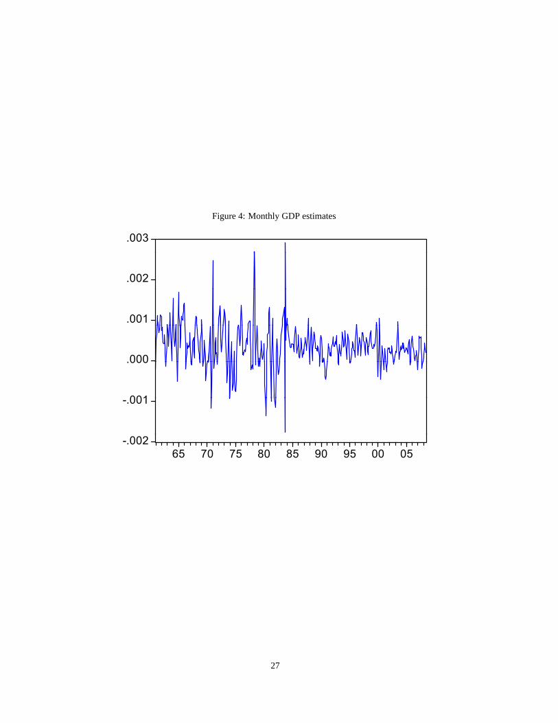
Figure 4: Monthly GDP estimates

.003

.002

.001

.000

001

.000

-.001

-.002

65 70 75 80 85 90 95 00 05

27