forecasting a large dimensional covariance matrix of a

Working Paper 01/2009 6 January 2009

FORECASTING A LARGE DIMENSIONAL COVARIANCE MATRIX OF A PORTFOLIO OF DIFFERENT ASSET CLASSES

Prepared by Lillie Lam, Laurence Fung and Ip-wing Yu1

Research Department

Abstract

In portfolio and risk management, estimating and forecasting the volatilities and correlations of asset returns plays an important role. Recently, interest in the estimation of the covariance matrix of large dimensional portfolios has increased. Using a portfolio of 63 assets covering stocks, bonds and currencies, this paper aims to examine and compare the predictive power of different popular methods adopted by i) market practitioners (such as the sample covariance, the 250-day moving average, and the exponentially weighted moving average); ii) some sophisticated estimators recently developed in the academic literature (such as the orthogonal GARCH model and the Dynamic Conditional Correlation model); and iii) their combinations. Based on five different criteria, we show that a combined forecast of the 250-day moving average, the exponentially weighted moving average and the orthogonal GARCH model consistently outperforms the other methods in predicting the covariance matrix for both one-quarter and one-year ahead horizons. JEL Classification Numbers: G17, G32, C52 Keywords: Volatility forecasting; Risk management; Portfolio management; Model evaluation Author’s E-Mail Addresses: [email protected], [email protected], [email protected]

1 The authors acknowledge the comments from Hans Genberg and Cho-hoi Hui.

The views and analysis expressed in this paper are those of the authors, and do not necessarily represent the views of the Hong Kong Monetary Authority.

- 2 -

EXECUTIVE SUMMARY:

Volatility modelling and forecasting are crucial in the financial market, given their important roles in option pricing, risk assessment and portfolio management. A better method to forecast the future volatilities and correlations of financial asset returns will definitely benefit portfolio managers and other financial market practitioners.

For investments covering various asset classes in different countries, recent research

has focused on developing an estimator of a covariance matrix of a large dimensional portfolio. This paper aims to examine and compare the predictive power of seven different methods that are found to perform well in terms of forecasting volatilities and correlations in the literature and widely applied by market practitioners. They include the orthogonal GARCH model, the Dynamic Conditional Correlation model, the sample covariance, the 250-day moving average, two exponential moving averages with two different weighting schemes and a combined forecast.

Using a portfolio of 63 assets from stocks, bonds and currencies in different

economies, we find that the combined forecast consistently outperforms the other six methods for both one-quarter and one-year ahead horizons. Despite the attractiveness of the combining forecasts shown in this study, it should be stressed that forecasting covariance of asset return is still a daunting task. The forecast of volatility and covariance of asset returns from combined forecast or any of these methods should be used with caution.

- 3 -

I. INTRODUCTION Volatility modelling and forecasting are important in the financial market, given its importance as a major input in option pricing, estimating the risk of assets and portfolio management. In fact, volatility itself has also become an underlying asset of the derivatives that are actively traded in the financial market, e.g. the variance swaps, the futures and options on the Chicago Board Options Exchange S&P500 Volatility Index (VIX). Unfortunately, despite its importance, volatility and correlation of financial asset returns are not directly observed and have to be derived from daily return data. A better way to forecast the future volatilities and correlations of financial asset returns will undoubtedly give portfolio managers and other financial market practitioners an edge in their decision making.

The importance of the variance and covariance has long been recognised in the finance literature and by financial market participants. Straightforward methods such as the sample covariance, the 250-day moving average and the exponentially weighted moving average have long been used and are still widely adopted. More sophisticated methods such as the family of GARCH models have also been extensively studied in the literature since 1990s. While univariate GARCH models are used to estimate the variance of the return of a single asset, multivariate GARCH models are developed for the covariance matrix of a portfolio. However, the large number of parameters in the estimation of the multivariate GARCH models posts practical problems in their implementation. To overcome this issue in the multivariate setting, Alexander and Chibumba (1997) and Alexander (2001) introduce the orthogonal GARCH (OGARCH) model based on univariate GARCH model and principal component analysis. The OGARCH model is computationally simpler than the multivariate GARCH models for a large dimensional covariance matrix and has achieved outstanding accuracy in forecasting correlation (Byström 2004). In addition to the OGARCH model, the Dynamic Conditional Correlation (DCC) model proposed by Engle (2002) for estimating a covariance matrix is also highlighted by recent studies. As shown in the literature, the DCC model captures the advantages of the GARCH models and simplifies the computation of the multivariate GARCH. Wong and Vlaar (2003) show that the DCC model has an outstanding performance in modelling time-varying correlations.

In the light of an increasing demand for estimating and forecasting the covariance matrix of a portfolio covering more than one asset class, a growing number of studies focus on developing an estimator of large dimensional covariance matrices (Bandi et al. 2008; Fleming et al. 2003; Andersen et al. 2005; and Bollerslev and Zhang 2003; Engle et al. 2008). As there are many methods to estimate the covariance matrix, there is a need to assess how these methods perform regarding their forecasts. The aim of this paper is to compare the forecasting performance of different models which are applied

- 4 -

either in the literature or by market practitioners to handle large dimensional covariance matrices. Altogether there are seven competing methods considered in this study, including the sample covariance, the 250-day moving average, two exponentially weighted moving averages, the OGARCH model, the DCC model and a combined forecast. Based on a portfolio of 63 assets covering stocks, bonds and currencies, the comparison examines the performance of these methods in forecasting the covariance matrix for one-quarter ahead and one-year ahead horizons. The model performance is assessed by their ability to forecast individual variance and covariance series under five different criteria. The remainder of this paper is organised as follows: Section 2 discusses the benchmark against which the forecasts are assessed. Section 3 outlines the seven competing estimators examined in this paper. The data involved and details of the estimations are described in Section 4. The criteria for evaluating the forecasts of the competing methods are presented in Section 5. The results on the forecast comparison are found in Section 6 and the conclusion follows in Section 7. II. BENCHMARK MEASURE: THE REALISED COVARIANCE MATRIX One of the difficulties to evaluate the performance of a covariance forecast is how to set a benchmark measure of the volatilities and correlations of asset returns. Andersen et al. (2003) has shown that the realised volatility measured by the sum of squared return is an unbiased and highly efficient estimator of return volatility. This measure has attracted much attention since then (Ederington and Guan 2004; Voev 2008; Andersen and Benzoni 2008). In this paper, we use this measure as the benchmark to assess the methods’ forecasting performance. Similar to Anderson et al. (2003), we calculate the h-day realised covariance matrix with its element at the ith row and jth column defined as

))((~1

, jjk

h

k

iik

jih rrrrV −−= ∑

=

(1)

where ikr (and j

kr ) is the return of asset i (and asset j) on day k; k = 1,…,h; ir is the

mean of the asset i’s daily returns over a period from day 1 to day h. It is noted that jiV ,~ is the variance of an individual asset’s return when

ji = and the covariance of the returns of two assets when ji ≠ .2 As there are 63 assets

2 The measure is similar to the original version used in Andersen et al. (2003) which calculates the

realised covariance matrix without subtracting the mean from the daily return. Both measures have been used in recent studies. In our study, we also tried the original definition of the realised covariance matrix as in Andersen et al. (2003) and found that the conclusion of this paper does not change. The estimation results using the definition of Andersen et al. (2003) are available upon request.

- 5 -

in our study and the matrix is positive-definite only when it is of full rank, the number of observation of each asset used in calculating the realised covariance matrix has to be at least 63, i.e. h ≥ 63. Specifically, in this paper, we estimate the covariance matrix for two different forecast horizons, the first one being one-quarter ahead by setting h = 63, and the second one being one-year ahead by taking h = 252. III. FORECASTING METHODS There are many methods to estimate the covariance matrix of a portfolio. In this paper, we compare the forecasting performance of the methods that are either widely adopted by market practitioners or recently developed in academic research. In addition, the methods selected should be suitable for estimating and forecasting large dimensional covariance matrices. In view of these criteria, a total of seven methods are considered in this study. They can be grouped into three categories. The first one is the sample covariance (SC), the 250-day moving average (MA) and the exponentially weighted moving averages with two different popular weighting schemes (EMA1 and EMA2). They are widely used by market practitioners. The second one is the OGARCH model introduced by Alexander and Chibumba (1997) and the DCC model proposed by Engle (2002). They are empirical models which are found to perform well in forecasting volatilities and correlations in the literature. The third one is a combined forecast of some of the above six methods.3 In the following section, we give a highlight of the various methods. 3.1 Sample Covariance (SC) Method The SC method uses all data available. At time t with a set of data from day t-T to t-1, the element at the ith row and jth column of the sample covariance matrix is defined as

)~)(~(1 1, jj

ki

t

Ttk

ik

jit rrrr

TSC −−= ∑

−

−=

(2)

where ir~ is the mean of an asset i’s return of a period from day t-T to t-1. At time t, the forecast of the covariance matrix for a period of h-day ahead based on the SC method is the product of tSC and h.4

3 The choice of the components in the combined forecast is based on the forecast power of individual

method. In this study, the MA, EMA2 and OGARCH methods are included in the combined forecast for evaluation.

4 To get a h-day covariance matrix from a one-day estimate, the common practice is to multiply the latter by h. See, for example, J.P. Morgan (1996) and Voev (2007).

- 6 -

3.2 250-day Moving Average (MA) Method This covariance matrix is determined in a similar way as the sample covariance method. The only difference is that it is based on the returns of the last 250 days. At time t with a set of data up to day t-1, the (i,j)th element of the covariance matrix given by the MA method is

∑−

−=

−−=1

250

, )~~)(~~(2501 t

tk

jjk

iik

jit rrrrMA (3)

where ir~~ is the mean of an asset i’s return for a period of last 250 days. At time t, the

forecast of the covariance matrix for a period of h-day ahead based on the MA method is the product of tMA and h.

3.3 Exponentially Weighted Moving Average Method The exponentially weighted moving average method is very popular among market practitioners. Unlike the methods of the SC and the MA which assign equal weights to every observation in the sample, the exponentially weighted moving average method attaches greater importance on the more recent observations. Two common weighting schemes are examined in this study, the EMA1 and EMA2, which are detailed in J.P. Morgan (1996) and Litterman and Winkelmann (1998) respectively.

For the EMA1 method, the (i,j)th element is given as

∑−

−=

−− −−−=1

111

, )~)(~()1(EMA1t

Ttk

jjk

iik

ktjit rrrrωω (4)

where 1ω is the decay factor and 10 1 << ω . The decay factor determines the importance of historical observations used for estimating the covariance matrix. The optimal value of the decay factor varies across different sample size and varying assets. Following J.P. Morgan (1996), a value of 0.94 for daily data is adopted in this paper for the EMA1. For the EMA2 method, the (i,j)th element is given as

)~()~(1EMA21

121

12

, jjk

t

Ttk

iik

ktt

Ttk

kt

jit rr −−= ∑

∑

−

−=

−−−

−=

−−

γγωω

(5)

The differences between EMA1 and EMA2 are: i) the value of the decay factor 2ω is

calibrated so that the only observations of the last five year are used, i.e. 02 ≈Tω when T =1260 which is about the total number of trading days in five years; and ii) a k-day

- 7 -

average of the daily return, tγ , instead of the daily return is used.5 In this study, the value

of k is 5, i.e. a 5-day average return is used in calculating the EMA2.6 For both EMA1 and EMA2, the forecast on the covariance matrix for the period of h-day ahead at time t is given by multiplying the tEMA by h in equations (4)

and (5) respectively.

3.4 Orthogonal GARCH (OGARCH) Model The merits of GARCH models in estimating variances are well documented in the literature. While the univariate GARCH model is easy to be implemented, the estimation of the multivariate GARCH models is not straight forward as they have to handle a massive number of parameters. For a portfolio of 63 assets, the number of parameters to be estimated in the covariance matrix is numerous. To overcome this problem in a multivariate setup, Ding (1994), Alexander and Chibumba (1997) and Alexander (2001) introduce the OGARCH model. Its main idea is to use the principal component analysis to generate a number of orthogonal factors that can be modelled in a univariate GARCH framework. Specifically for a set of N asset return series with T observations, represented by a NT × matrix tR , its principal components ( tP ) are given by the NT ×

matrix as

ttt WRP = (6)

where tW is an orthogonal NN × matrix of the eigenvectors of tt RR′ arranged in

descending order of the corresponding eigenvalues. Multiplying both sides of equation (6) by tW ′ (the transpose of tW ), the set of return series can be written in terms of

principal components as:

ttt WPR ′= (7)

At time t, the covariance matrix of tR ( tOG ) is calculated as:

ttttttttt WDWWPWWPOG ′=′=′= )var()var( (8)

5 As suggested by J.P. Morgan (1996), the decay factor in this paper is calibrated using 01.02 =Tω . 6 As suggested by Litterman and Winkelmann (1998), averaging the data in this manner can help

removing the undesirable noise in the daily data. Popular choices of k are 5 (i.e. a weekly average) and 22 (i.e. a monthly average). We have tried both k = 5 and k = 22 in our study and found that the resulting covariance matrix based on k = 5 performs better in forecasting. The results for comparison are available upon request.

- 8 -

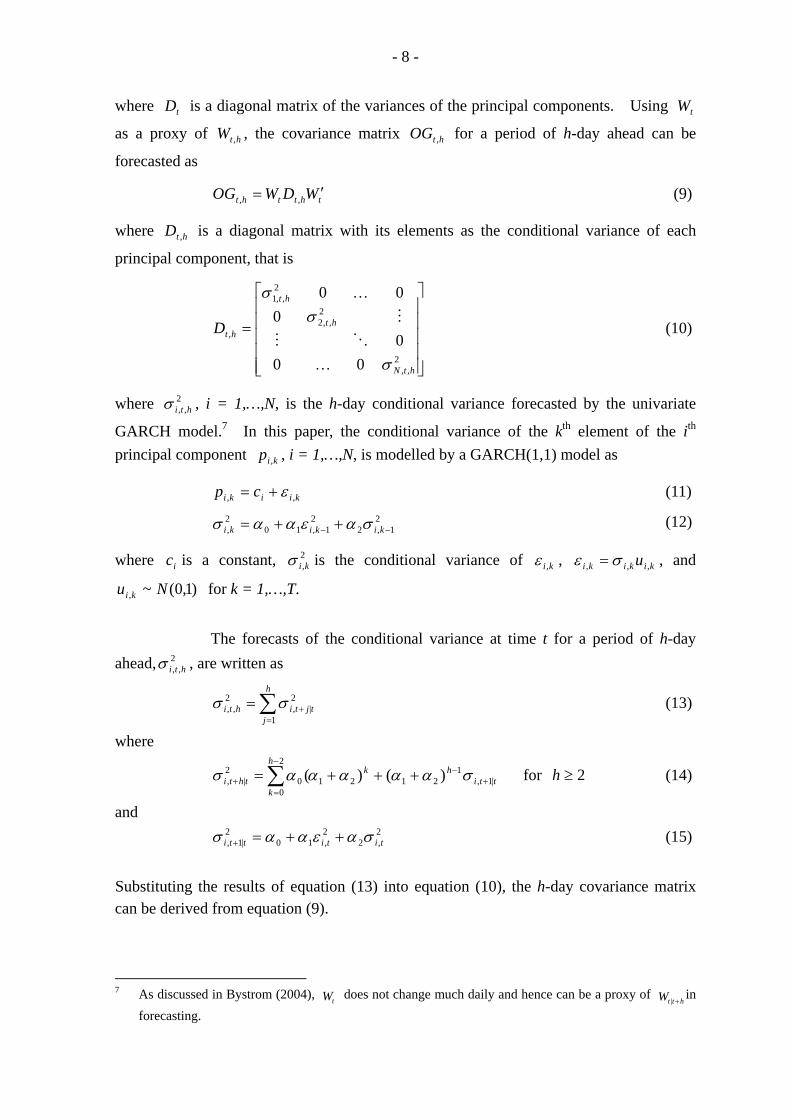
where tD is a diagonal matrix of the variances of the principal components. Using tW

as a proxy of htW , , the covariance matrix htOG , for a period of h-day ahead can be

forecasted as

thttht WDWOG ′= ,, (9)

where htD , is a diagonal matrix with its elements as the conditional variance of each

principal component, that is

⎥⎥⎥⎥⎥

⎦

⎤

⎢⎢⎢⎢⎢

⎣

⎡

=

2,,

2,,2

2,,1

,

000

000

htN

ht

ht

htD

σ

σσ

K

OM

M

K

(10)

where 2,, htiσ , i = 1,…,N, is the h-day conditional variance forecasted by the univariate

GARCH model.7 In this paper, the conditional variance of the kth element of the ith principal component kip , , i = 1,…,N, is modelled by a GARCH(1,1) model as

kiiki cp ,, ε+= (11)

2

1,22

1,102, −− ++= kikiki σαεαασ (12)

where ic is a constant, 2,kiσ is the conditional variance of ki,ε , kikiki u ,,, σε = , and

)1,0(~, Nu ki for k = 1,…,T.

The forecasts of the conditional variance at time t for a period of h-day ahead, 2

,, htiσ , are written as

∑=

+=h

jtjtihti

1

2|,

2,, σσ (13)

where

ttihk

h

kthti |1,

12121

2

00

2|, )()( +

−−

=+ +++= ∑ σααααασ for 2≥h (14)

and 2

,22,10

2|1, tititti σαεαασ ++=+ (15)

Substituting the results of equation (13) into equation (10), the h-day covariance matrix can be derived from equation (9). 7 As discussed in Bystrom (2004), tW does not change much daily and hence can be a proxy of

httW +|in

forecasting.

- 9 -

3.5 Dynamic Conditional Correlation (DCC) Model The DCC model, proposed by Engle and Sheppard (2001) and Engle (2002), is a new class of multivariate models which is particularly well suited to examine correlation dynamics among assets. The DCC model has the flexibility of a univariate GARCH model but without the complexity of a general multivariate GARCH model. As the parameters to be estimated in the correlation process are independent of the number of series to be correlated, a large number of series can be considered in a single estimation. Furthermore, Wong and Vlaar (2003) show that the DCC model outperforms other alternatives in modelling time-varying covariance. Empirically, the DCC model assumes that a set of N asset returns and T observations are conditionally multivariate normal with mean zero and a covariance matrix tDCC . In the DCC model, the set of asset

returns tR is first filtered and the residuals after the filtering process are assumed to be

distributed as

),0(~| 1 ttt DCCNFR − (16)

and

tttt HHDCC Ψ= (17)

where tH is a NN × diagonal matrix of time varying standard deviations from

univariate GARCH models, tΨ is the time varying correlation matrix and 1−tF is a

filtering process.8 In this paper, the time varying standard deviation is modelled by a GARCH (1,1) model as

1,22

1,10,~~

−− ++= tititi hrh βββ (18)

where tih ,~ is the ith diagonal element of tH , tir , is the element on the ith row and tth

column of 'tR , i = 1,…,N and t = 1,…,T. The dynamic correlation structure is modelled

as DCC(1,1) in the form of

1211121 )()1( −−− +′+−−= tttt QQQ φυυφφφ (19)

and

11 −∗−∗=Ψ tttt QQQ (20)

8 Following Engle and Sheppard (2001), the filtering process is performed by first regressing the return

series on a constant and then applying the residuals from the regression to the DCC model with distribution as ),0( tDCCN .

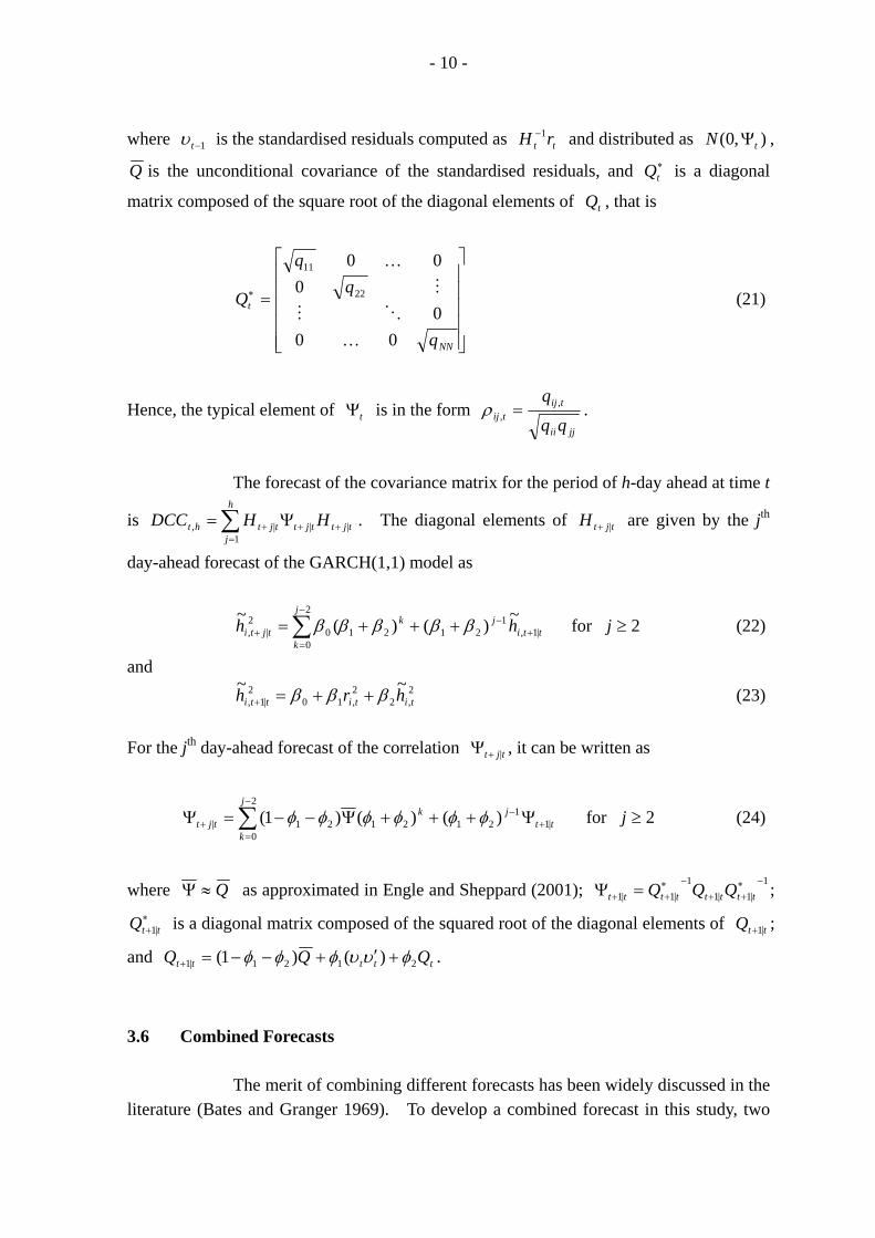
- 10 -

where 1−tυ is the standardised residuals computed as tt rH 1− and distributed as ),0( tN Ψ ,

Q is the unconditional covariance of the standardised residuals, and ∗tQ is a diagonal

matrix composed of the square root of the diagonal elements of tQ , that is

⎥⎥⎥⎥⎥

⎦

⎤

⎢⎢⎢⎢⎢

⎣

⎡

=∗

NN

t

q

qq

Q

000

000

22

11

K

OM

M

K

(21)

Hence, the typical element of tΨ is in the form jjii

tijtij qq

q ,, =ρ .

The forecast of the covariance matrix for the period of h-day ahead at time t

is ∑=

+++ Ψ=h

jtjttjttjtht HHDCC

1|||, . The diagonal elements of tjtH |+ are given by the jth

day-ahead forecast of the GARCH(1,1) model as

ttijk

j

ktjti hh |1,

12121

2

00

2|,

~)()(~+

−−

=+ +++= ∑ βββββ for 2≥j (22)

and 2

,22,10

2|1,

~~tititti hrh βββ ++=+ (23)

For the jth day-ahead forecast of the correlation tjt |+Ψ , it can be written as

∑−

=+

−+ Ψ+++Ψ−−=Ψ

2

0|1

1212121| )()()1(

j

ktt

jktjt φφφφφφ for 2≥j (24)

where Q≈Ψ as approximated in Engle and Sheppard (2001); 1|1|1

1|1|1

−∗++

−∗++ =Ψ tttttttt QQQ ;

∗+ ttQ |1 is a diagonal matrix composed of the squared root of the diagonal elements of ttQ |1+ ;

and ttttt QQQ 2121|1 )()1( φυυφφφ +′+−−=+ .

3.6 Combined Forecasts The merit of combining different forecasts has been widely discussed in the literature (Bates and Granger 1969). To develop a combined forecast in this study, two

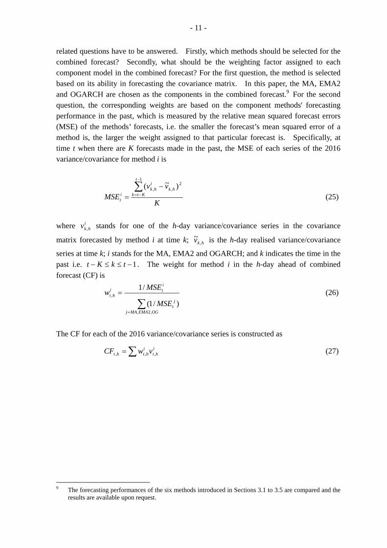
- 11 -

related questions have to be answered. Firstly, which methods should be selected for the combined forecast? Secondly, what should be the weighting factor assigned to each component model in the combined forecast? For the first question, the method is selected based on its ability in forecasting the covariance matrix. In this paper, the MA, EMA2 and OGARCH are chosen as the components in the combined forecast.9 For the second question, the corresponding weights are based on the component methods' forecasting performance in the past, which is measured by the relative mean squared forecast errors (MSE) of the methods’ forecasts, i.e. the smaller the forecast’s mean squared error of a method is, the larger the weight assigned to that particular forecast is. Specifically, at time t when there are K forecasts made in the past, the MSE of each series of the 2016 variance/covariance for method i is

K

vvMSE

t

Ktkhk

ihk

it

∑−

−=

−=

12

,, )~( (25)

where i

hkv , stands for one of the h-day variance/covariance series in the covariance

matrix forecasted by method i at time k; hkv ,~ is the h-day realised variance/covariance

series at time k; i stands for the MA, EMA2 and OGARCH; and k indicates the time in the past i.e. 1−≤≤− tkKt . The weight for method i in the h-day ahead of combined forecast (CF) is

∑=

=

OGEMAMAj

jt

iti

ht

MSE

MSEw

,2,

,

)/1(

/1 (26)

The CF for each of the 2016 variance/covariance series is constructed as

∑= iht

ihtht vwCF ,,, (27)

9 The forecasting performances of the six methods introduced in Sections 3.1 to 3.5 are compared and the

results are available upon request.

- 12 -

IV. DATA AND ESTIMATION 4.1 Data In this study, we consider the asset allocation decision of international investors on the global market portfolio of equities and bonds. As the hedging of foreign exchange risk in an international portfolio is important, the global market portfolio also includes foreign currency investment. Since the extent of currency hedging varies among investors, we follow Black and Litterman (1991) by applying an 80% hedging ratio in our study. For empirical estimation, the global portfolio is assumed to track major economies’ market indices, for example, the equity component is covered by the MSCI International Equity Indices and the bond component by the JP Morgan Government Bond Indices or the Citigroup World Government Bond Indices. For the hedging of foreign exchange risk, the foreign currency investments are those that reflect the country exposure of either equities or bonds in the portfolio. Daily data of excess returns of assets in three different classes, namely equities, fixed incomes and currencies, from 30 January 1998 to 31 October 2007 are studied in this paper.10 Altogether, there are 63 assets in the global market portfolio (Table 1 lists the corresponding economies / markets of these 63 assets). All data are collected from Datastream and DataQuery of J.P. Morgan.

10 As most of the investors care about the returns of the investment in excess of the risk-free rate, our study

focuses on the volatility and covariance of excess asset returns. Refer to Black and Litterman (1991) for more discussion.

- 13 -

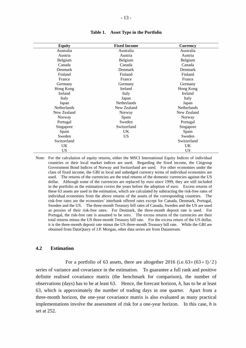
Table 1. Asset Type in the Portfolio

Equity Fixed Income Currency

Australia Australia Australia Austria Austria Austria Belgium Belgium Belgium Canada Canada Canada

Denmark Denmark Denmark Finland Finland Finland France France France

Germany Germany Germany Hong Kong Ireland Hong Kong

Ireland Italy Ireland Italy Japan Italy Japan Netherlands Japan

Netherlands New Zealand Netherlands New Zealand Norway New Zealand

Norway Spain Norway Portugal Sweden Portugal

Singapore Switzerland Singapore Spain UK Spain

Sweden US Sweden Switzerland Switzerland

UK UK US US

Note: For the calculation of equity returns, either the MSCI International Equity Indices of individual countries or their local market indices are used. Regarding the fixed income, the Citigroup Government Bond Indices of Norway and Switzerland are used. For other economies under the class of fixed income, the GBI in local and unhedged currency terms of individual economies are used. The returns of the currencies are the total returns of the domestic currencies against the US dollar. Although some of the currencies are replaced by euro since 1999, they are still included in the portfolio as the estimation covers the years before the adoption of euro. Excess returns of these 63 assets are used in the estimation, which are calculated by subtracting the risk-free rates of individual economies from the above returns of the assets of the corresponding countries. The risk-free rates are the economies’ interbank offered rates except for Canada, Denmark, Portugal, Sweden and the US. The three-month Treasury bill rates of Canada, Sweden and the US are used as proxies of their risk-free rates. For Denmark, the three-month deposit rate is used. For Portugal, the risk-free rate is assumed to be zero. The excess returns of the currencies are their total returns minus the US three-month Treasury bill rate. For the excess return of the US dollar, it is the three-month deposit rate minus the US three-month Treasury bill rate. While the GBI are obtained from DataQuery of J.P. Morgan, other data series are from Datastream.

4.2 Estimation For a portfolio of 63 assets, there are altogether 2016 (i.e. 2/)163(63 +× ) series of variance and covariance in the estimation. To guarantee a full rank and positive definite realised covariance matrix (the benchmark for comparison), the number of observations (days) has to be at least 63. Hence, the forecast horizon, h, has to be at least 63, which is approximately the number of trading days in one quarter. Apart from a three-month horizon, the one-year covariance matrix is also evaluated as many practical implementations involve the assessment of risk for a one-year horizon. In this case, h is set at 252.

- 14 -

A recursive estimation is carried out for the data with the first one using the information from January 1998 to December 2002. The ex-post forecasting period starts from January 2003 and ends in October 2007. For a one-quarter ahead horizon, the first ex-post forecast is estimated using data from 31 January 1998 to 31 December 2002 and is a forecast for a covariance matrix for a period of 63 days starting from 1 January 2003. The second ex-post forecast is estimated using data from 31 January 1998 to 31 January 2003 and is the one for a period of 63 days starting from 1 February 2003, and so on. The last ex-post forecast estimation uses data from 31 January 1998 to 31 July 2007 and this is used to forecast the covariance matrix for a period of 63 days starting from 1 August 2007. In total, there are 56 ex-post forecasts for evaluation for a one-quarter ahead horizon.

Similar procedures are applied to the estimation of the forecast for the one-year covariance matrix. The first estimation uses data from 31 January 1998 to 31 December 2002 and the first ex-post forecast is the forecast for a one-year covariance matrix for the period from January 2003 to December 2003. Data is updated to 31 January 2003 for the second estimation and the second ex-post forecast is the forecast for a one-year ahead covariance matrix for the period from February 2003 to January 2004. The last one-year ahead forecast is the one for the period from November 2006 to October 2007 with its estimation based on the data from 31 January 1998 to 31 October 2006. There are altogether 47 ex-post forecasts for the evaluation in this case. V. FORECAST EVALUATION CRITERIA Five different criteria are used to evaluate the ex-post forecasts in this study. They are: 5.1 Root Mean Squared Forecast Error (RMSE) For each element in the covariance matrix, the RMSE is defined as

∑=

−=K

k

jik

jik VV

KRMSE

1

2,, )~(1 (28)

where jiV , is the (i,j)th element of the covariance matrix forecasted by the methods

specified in Section 2; jiV ,~ is the corresponding element of the realised covariance matrix; K is the total number of ex-post forecasts which equals to 56 for the evaluation of the forecasts of the quarterly covariance matrix and 47 for that of the annual one. For each of the 2016 variance/covariance series, its RMSE is compared and ranked among the seven forecasting methods. The method which has the most series at the top ranks is preferred under this criterion.

- 15 -

5.2 Diebold-Mariano Test (DM test) This test, introduced by Diebold and Mariano (1995), compares the forecasting methods in pair. The null is to test whether two competing methods have equal forecasting accuracy. A rejection of the null suggests that one of the forecasting methods is statistically different from the other. The Diebold-Mariano test statistic (DM statistic) is derived based on a loss function kd which is defined as

2,

2, kjkik eed −= , k = 1, …,K (29)

where kie , and kje , are respectively the errors of the kth ex-post forecast of two

competing methods i and j. The DM statistic is then given as

)(dse

dDM = (30)

where d is the mean of the loss function d and )(dse is the standard error of d . Under the null hypothesis, the DM statistic has an asymptotic normal distribution. If the squared forecast error of method i is statistically less than that of method j at the 5% significance level, then method i is said to outperform method j. The comparison is taken for each of 2016 series in the covariance matrix. The method which has consistently outperformed the other is considered a better method under this criterion. 5.3 Hypothesis Testing of Regression Coefficient This criterion is to see whether the forecasts of different methods are closely correlated with the realised variance/covariance in a regression set up. To do this, the realised variance/covariance series is first regressed on the forecast of the variance/covariance series from the forecasting methods in the following form: t

itt vv εββ ++= 10

~ (31)

where iv is the forecast variance/covariance series by method i; i represents different forecasting method. Student’s t test is carried out on the coefficient with the null hypothesis set as 1β =1. The comparison is based on how many series (out of 2016) are rejected in the hypothesis testing at the common significance levels. The smaller the number is, the more preferable the method is. 5.4 Direction of Change The criterion is to examine whether the forecast will move in the same direction as the realised value. For each ex-post forecasting period, a ‘one’ will be assigned for the period when the method predicts correctly the direction of the realised variance/covariance movement and zero otherwise. The comparison is based on the

- 16 -

number and the proportion of series predicting the direction correctly. The larger the number is, the better the forecasting method is. 5.5 Sign of Covariance While the variance carries a positive sign, the covariance can be either positive or negative. As different signs may have different impacts on portfolio allocation, the test on which method is able to give a correct sign of covariance is also important for model evaluation. In this test, the signs of the covariance predicted by the forecasting methods are evaluated by comparing with those of the realised covariance. For each ex-post forecasting period, the criterion is to examine whether the forecast will give the same sign as the realised value. The higher the number and the proportion are, the better the method is. VI. RESULTS This section evaluates the ex-post forecasts of the covariance matrices for one-quarter ahead and one-year ahead horizons based on the five criteria described in Section 5. Tables 2 to 6 give the results of the quarterly covariance matrix and Tables 7 to 11 show the results of the annual one. For better illustration, we plot the realised variance/covariance series along with the forecasts of the seven methods of the representative cases in Charts 1 to 4 for the quarterly forecast horizon and in Charts 5 to 8 for the annual one. In these graphs, the variance/covariance series are divided into six combinations according to different pairs from the three classes of the assets included in this paper: the equity-equity, the equity-fixed income, the equity-currency, the fixed income-fixed income, the fixed income-currency, and the currency-currency. 6.1 Covariance Forecast for One-Quarter Ahead Horizon Table 2 shows the ranking of the seven methods given by the RMSE criterion for each of 2016 series of the variance and covariance in the matrix. For each forecast, rank ‘one’ is given to the method with the smallest RMSE while rank ‘seven’ is assigned to the one with the largest RMSE. Using the RMSE as the criterion, the method with more series ranked the first is preferred. As shown in Table 2, about half of the 2016 series predicted by the CF method rank the first. The CF method also has the most series ranked the second.

- 17 -

Table 2. Ranking of One-Quarter Ahead Forecast from Different Methods based on RMSE

Rank SC MA EMA1 EMA2 OGARCH DCC CF 1 131 369 142 135 106 151 982 2 141 562 158 157 344 80 574 3 211 267 406 219 393 207 313 4 293 201 195 350 523 330 124 5 418 190 270 260 451 405 22 6 430 232 239 367 179 568 1 7 392 195 606 528 20 275 0

Note: The root-mean-squared-error (RMSE) of each method’s forecasts of the 2016 series is ranked in an ascending order. The smallest RMSE ranks ‘one’ and the largest RMSE is with a rank of ‘seven’. The entry in each cell corresponds to the number of series (out of 2016 series) that each method is placed under different rankings.

Under the DM test presented in Table 3, the forecasts of the CF method outperform those given by the other six methods. The DM test evaluates the methods in pair. The left–hand-side entry of each cell in Table 3 is the number of the outperforming series (out of 2016 series) based on the method given by the corresponding column over the method given by the corresponding row. The right-hand-side entry of each cell is the number of series, out of the number of series in the left-hand-side entry, being significant at the 5% level. As shown in Table 3, the CF method beats all other methods with the largest number of outperforming series, amounting at least 75% of the 2016 series. The number of significant outperforming series of the CF method is also the largest among all the methods. Based on the DM test, we find that the CF test significantly outperforms the other six methods.

Table 3. Results of DM Test on One-Quarter Ahead Forecast from Different Methods

SC MA EMA1 EMA2 OGARCH DCC CF SC - 1377 / 561 1049 / 252 939 / 233 1515 / 743 999 / 187 1737 / 1042

MA 639 / 47 - 534 / 0 742 / 61 795 / 33 622 / 16 1457 / 132

EMA1 967 / 296 1482 / 453 - 925 / 360 1307 / 411 992 / 393 1793 / 741

EMA2 1077 / 457 1274 / 575 1091 / 537 - 1446 / 633 975 / 316 1825 / 823

OGARCH 501 / 99 1221 / 143 709 / 94 570 / 149 - 690 / 62 1827 / 825

DCC 1017 / 230 1394 / 247 1024 / 204 1041 / 176 1326 / 294 - 1792 / 587

CF 279 / 29 559 / 0 223 / 0 191 / 34 189 / 24 224 / 1 -

Note: The left-hand-side entry in each cell is the number of series (out of 2016) that the model in the corresponding column outperforms the model in the corresponding row in terms of root-mean-squared-error. The right-hand-side entry in each cell is the number of series that the outperformance is significant according to the DM test at the 5% significance level.

For the regression set up as in Section 5.3, the coefficient 1β measures how the forecast series of variance and covariance are able to predict the realised ones.

- 18 -

Results on testing whether the coefficients given by different methods in the regression as shown in equation (31) that are significantly different from one (i.e. the null is 1: 10 =βH )

are reported in Table 4. As shown in Table 4, the CF test has the least number of cases rejected in the hypothesis testing at the 1%, 5%, and 10% significance levels. This reflects that the CF method has the best performance among all other methods in forecasting the realised covariance matrix.

Table 4. Number of Series of One-Quarter Ahead Forecast Rejected in the Regression Test

Significance Levels SC MA EMA1 EMA2 OGARCH DCC CF

1% 1021 1129 1924 924 542 1373 254 5% 1270 1398 1981 1201 734 1678 687 10% 1389 1498 1989 1326 904 1765 847

Note: The number corresponds to the total number of forecast series (out of 2016 series) rejected in the hypothesis testing of 11 =β in the regression t


~ as specified in equation (31).

Table 5 indicates how different forecasting methods perform under the criteria of direction of change. As shown in Table 5, about 80% of the series forecasted by the CF method predict the direction of change correctly while the percentages of other methods range from 69% to 77% only.

Table 5. Results of the Test on the Direction of Change for One-Quarter Ahead Forecast

SC MA EMA1 EMA2 OGARCH DCC CF 68246 71846 65415 71810 72924 71620 76684

72.03% 75.83% 69.04% 75.79% 76.96% 75.59% 80.93%

Note: The entries in the first and the second rows give, respectively, the number and the percentage of forecasts that the direction of change given by the forecast is same as the realised covariance. There are a total of 112896 forecasts (56 ex-post forecasts times 2016 series of variances and covariance) in the comparison for each method.

Finally, Table 6 shows whether the forecasts have correctly predicted the sign of covariance. As shown in Table 6, all methods demonstrate their outstanding powers as each method correctly predicts the sign of covariance for at least 90% of times. In particular, the CF, the EMA2 and the MA methods are the best as they are able to predict the sign correctly for about 98% of times.

Overall, after considering all five criteria, the results suggest that the CF method consistently performs better than the other methods in forecasting the one-quarter ahead covariance matrix.

- 19 -

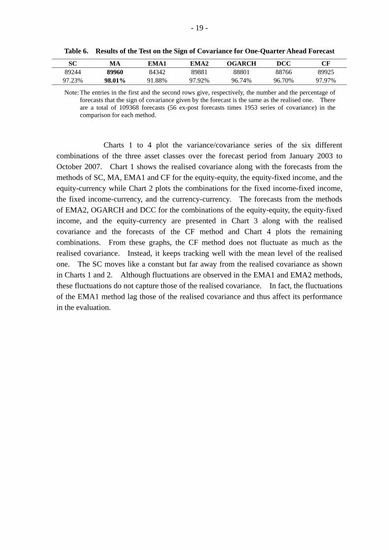
Table 6. Results of the Test on the Sign of Covariance for One-Quarter Ahead Forecast


97.23% 98.01% 91.88% 97.92% 96.74% 96.70% 97.97%

Note: The entries in the first and the second rows give, respectively, the number and the percentage of forecasts that the sign of covariance given by the forecast is the same as the realised one. There are a total of 109368 forecasts (56 ex-post forecasts times 1953 series of covariance) in the comparison for each method.

Charts 1 to 4 plot the variance/covariance series of the six different combinations of the three asset classes over the forecast period from January 2003 to October 2007. Chart 1 shows the realised covariance along with the forecasts from the methods of SC, MA, EMA1 and CF for the equity-equity, the equity-fixed income, and the equity-currency while Chart 2 plots the combinations for the fixed income-fixed income, the fixed income-currency, and the currency-currency. The forecasts from the methods of EMA2, OGARCH and DCC for the combinations of the equity-equity, the equity-fixed income, and the equity-currency are presented in Chart 3 along with the realised covariance and the forecasts of the CF method and Chart 4 plots the remaining combinations. From these graphs, the CF method does not fluctuate as much as the realised covariance. Instead, it keeps tracking well with the mean level of the realised one. The SC moves like a constant but far away from the realised covariance as shown in Charts 1 and 2. Although fluctuations are observed in the EMA1 and EMA2 methods, these fluctuations do not capture those of the realised covariance. In fact, the fluctuations of the EMA1 method lag those of the realised covariance and thus affect its performance in the evaluation.

- 20 - Chart 1. Comparison of the one-quarter ahead forecast of covariance of the equity-equity, the equity-fixed income, the equity-currency by the methods of sample covariance (SC),

the 250-day moving average (MA), the exponentially weighted moving average (EMA1) and the combined forecast (CF) with their realised covariance from January-March 2003 to August-October 2007

Covariance of the Equity-Equity Covariance of the Equity-Fixed Income Covariance of the Equity-Currency New Zealand Equity_Switzerland Equity

-0.0015

-0.0010

-0.0005

0.0000

0.0005

0.0010

0.0015

0.0020

0.0025

Jan-03 Jun-03 Nov-03 Apr-04 Sep-04 Feb-05 Jul-05 Dec-05 May-06 Oct-06 Mar-07 Aug-07

Realised Covariance SC MA EMA1 CF

US Equity_Japan Fixed Income

-0.0005

-0.0004

-0.0003

-0.0002

-0.0001

0.0000

0.0001

0.0002

0.0003



Portugal Equity_US Dollar

-2.0E-06

-1.5E-06

-1.0E-06

-5.0E-07

0.0E+00

5.0E-07

1.0E-06

1.5E-06

2.0E-06

2.5E-06

3.0E-06



Singapore Equity_US Equity

-0.002

-0.001

0.000

0.001

0.002

0.003

0.004

0.005

0.006



New Zealand Equity_Switzerland Fixed Income

-0.0006

-0.0005

-0.0004

-0.0003

-0.0002

-0.0001

0.0000

0.0001

0.0002

0.0003

0.0004



Switzerland Equity_Singapore Dollar

-0.0020

-0.0015

-0.0010

-0.0005

0.0000

0.0005

0.0010

0.0015



Canada Equity_Portugal Equity

-0.002

-0.001

0.000

0.001

0.002

0.003

0.004

0.005



Canada Equity_Australia Fixed Income

-0.0005

-0.0004

-0.0003

-0.0002

-0.0001

0.0000

0.0001

0.0002

0.0003

0.0004



Canada Equity_Swiss Franc

-0.0025

-0.0020

-0.0015

-0.0010

-0.0005

0.0000

0.0005

0.0010

0.0015

0.0020



- 21 - Chart 2. Comparison of the one-quarter ahead forecast of covariance of the fixed income-fixed income, the fixed income-currency, the currency-currency by the methods of

sample covariance (SC), the 250-day moving average (MA), the exponentially weighted moving average (EMA1) and the combined forecast (CF) with their realised covariance from January-March 2003 to August-October 2007

Covariance of the Fixed Income-Fixed Income Covariance of the Fixed Income-Currency Covariance of the Currency-Currency Australia Fixed Income_Switzerland Fixed Income

-0.00010

-0.00005

0.00000

0.00005

0.00010

0.00015

0.00020

0.00025

0.00030



Finland Fixed Income_US Dollar

-4.E-07

-3.E-07

-2.E-07

-1.E-07

0.E+00

1.E-07

2.E-07

3.E-07

4.E-07

5.E-07



US Dollar_Hong Kong Dollar

-2.0E-07

-1.5E-07

-1.0E-07

-5.0E-08

0.0E+00

5.0E-08

1.0E-07

1.5E-07

2.0E-07

2.5E-07

3.0E-07

3.5E-07


Realised Covariance SC MA EMA1 CF Finland Fixed Income_New Zealand Fixed Income

-0.00005

0.00000

0.00005

0.00010

0.00015

0.00020

0.00025

0.00030

0.00035



Denmark Fixed Income_Hong Kong Dollar

-0.00001

0.00000

0.00001

0.00002

0.00003

0.00004

0.00005



Singapore Dollar_Singapore Dollar

0.0000

0.0002

0.0004

0.0006

0.0008

0.0010

0.0012

0.0014

0.0016

0.0018


Realised Covariance SC MA EMA1 CF Canada Fixed Income_Sweden Fixed Income

0.00000

0.00005

0.00010

0.00015

0.00020

0.00025

0.00030

0.00035

0.00040



Norway Fixed Income_Singapore Dollar

-0.00020

-0.00015

-0.00010

-0.00005

0.00000

0.00005

0.00010

0.00015

0.00020

0.00025

0.00030



Japanese Yen_Irish Pound

-0.0005

0.0000

0.0005

0.0010

0.0015

0.0020

0.0025



- 22 - Chart 3. Comparison of the one-quarter ahead forecast of covariance of the equity-equity, the equity-fixed income, the equity-currency by the methods of the exponentially

weighted moving average (EMA2), the orthogonal GARCH model (OGARCH), the Dynamic Conditional Correlation model (DCC) and the combined forecast (CF) with their realised covariance from January-March 2003 to August-October 2007

Covariance of the Equity-Equity Covariance of the Equity-the Fixed Income Covariance of the Equity-Currency

New Zealand Equity_Switzerland Equity

-0.0010

-0.0005

0.0000

0.0005

0.0010

0.0015

0.0020

0.0025


Realised Covariance EMA2 OGARCH DCC CF

US Equity_Japan Fixed Income

-0.00045

-0.00040

-0.00035

-0.00030

-0.00025

-0.00020

-0.00015

-0.00010

-0.00005

0.00000

0.00005

0.00010



Portugal Equity_US Dollar

-1.5E-06

-1.0E-06

-5.0E-07

0.0E+00

5.0E-07

1.0E-06

1.5E-06

2.0E-06

2.5E-06

3.0E-06



Singapore Equity_US Equity

-0.0015

-0.0010

-0.0005

0.0000

0.0005

0.0010

0.0015

0.0020

0.0025

0.0030

0.0035

0.0040



New Zealand Equity_Switzerland Fixed Income

-0.0006

-0.0005

-0.0004

-0.0003

-0.0002

-0.0001

0.0000

0.0001

0.0002

Jan-03 Jun-03 Nov-03 Apr-04 Sep-04 Feb-05 Jul-05 Dec-05 May-06 Oct-06 Mar-07 Aug-07Realised Covariance EMA2 OGARCH DCC CF

Switzerland Equity_Singapore Dollar

-0.0015

-0.0010

-0.0005

0.0000

0.0005

0.0010

0.0015



Canada Equity_Portugal Equity

-0.002

-0.001

0.000

0.001

0.002

0.003

0.004

0.005

0.006

0.007



Canada Equity_Australia Fixed Income

-0.0004

-0.0003

-0.0002

-0.0001

0.0000

0.0001

0.0002

0.0003



Canada Equity_Swiss Franc

-0.0020

-0.0015

-0.0010

-0.0005

0.0000

0.0005

0.0010

0.0015



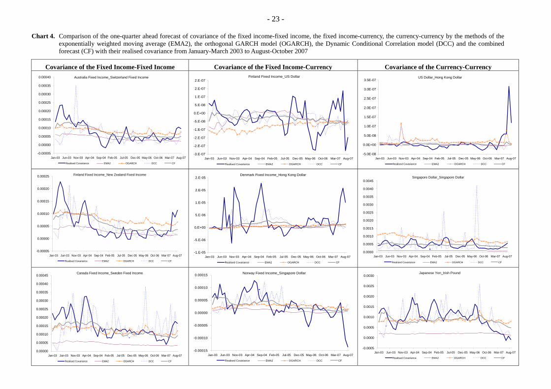
- 23 - Chart 4. Comparison of the one-quarter ahead forecast of covariance of the fixed income-fixed income, the fixed income-currency, the currency-currency by the methods of the

exponentially weighted moving average (EMA2), the orthogonal GARCH model (OGARCH), the Dynamic Conditional Correlation model (DCC) and the combined forecast (CF) with their realised covariance from January-March 2003 to August-October 2007

Covariance of the Fixed Income-Fixed Income Covariance of the Fixed Income-Currency Covariance of the Currency-Currency Australia Fixed Income_Switzerland Fixed Income

-0.00005

0.00000

0.00005

0.00010

0.00015

0.00020

0.00025

0.00030

0.00035

0.00040



Finland Fixed Income_US Dollar

-3.E-07

-2.E-07

-2.E-07

-1.E-07

-5.E-08

0.E+00

5.E-08

1.E-07

2.E-07

2.E-07




-5.0E-08

0.0E+00

5.0E-08

1.0E-07

1.5E-07

2.0E-07

2.5E-07

3.0E-07

3.5E-07



Finland Fixed Income_New Zealand Fixed Income

-0.00005

0.00000

0.00005

0.00010

0.00015

0.00020

0.00025



Denmark Fixed Income_Hong Kong Dollar

-1.E-05

-5.E-06

0.E+00

5.E-06

1.E-05

2.E-05

2.E-05



Singapore Dollar_Singapore Dollar

0.0000

0.0005

0.0010

0.0015

0.0020

0.0025

0.0030

0.0035

0.0040

0.0045


Realised Covariance EMA2 OGARCH DCC CF Canada Fixed Income_Sweden Fixed Income

0.00000

0.00005

0.00010

0.00015

0.00020

0.00025

0.00030

0.00035

0.00040

0.00045



Norway Fixed Income_Singapore Dollar

-0.00015

-0.00010

-0.00005

0.00000

0.00005

0.00010

0.00015



Japanese Yen_Irish Pound

-0.0005

0.0000

0.0005

0.0010

0.0015

0.0020

0.0025

0.0030



- 24 -

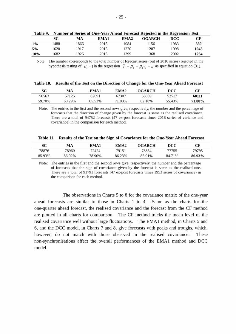
6.2 Covariance Forecast for One-Year Ahead Horizon Tables 7 to 11 give the evaluation of the performances of the seven methods in forecasting the one-year ahead covariance matrix. In Table 7, the number of series (1281 out of 2016 series) ranked the first for the CF method is significantly more than those for the other methods. Both results from the DM test and the hypothesis testing of the regression coefficient in Tables 8 and 9 are similar to those of the one-quarter ahead forecast on the covariance matrix. The CF method has the best performances under these two criteria. Same as the shorter horizon, the CF method is the one with the most forecasts in correct direction. As shown in Table 10, 72% of the forecast from the CF method predict the direction correctly. While the MA method has performed as well as the CF method for forecasting the sign of covariance at one-quarter ahead horizon, the latter is found to be superior for the one-year ahead horizon. As shown in Table 11, 87% of the forecasts from the CF method give the same sign as the realised one.

Table 7. Ranking of One-Year Ahead Forecast from Different Methods Based on RMSE

Rank SC MA EMA1 EMA2 OGARCH DCC CF 1 188 40 29 354 91 33 1281 2 141 383 37 594 336 46 479 3 258 265 229 141 774 151 198 4 496 428 170 142 422 302 56 5 423 267 434 126 250 514 2 6 251 272 392 170 134 797 0 7 259 361 725 489 9 173 0

Note: The root-mean-squared-error (RMSE) of each method’s forecasts of the 2016 series is ranked in ascending order. The smallest RMSE ranks ‘one’ and the largest RMSE is with a rank of ‘seven’. The entry in each cell corresponds to the number of series (out of 2016 series) that each method is placed under different rankings.

Table 8. Results of DM Test on the One-Year Ahead Forecast from Different Methods

SC MA EMA1 EMA2 OGARCH DCC CF SC - 951 / 148 640 / 98 1103 / 675 1547 / 832 665 / 221 1740 / 1202

MA 1065 / 81 - 518 / 3 1196 / 92 1283 / 56 783 / 3 1946 / 262

EMA1 1376 / 501 1498 / 417 - 1402 / 614 1597 / 563 1196 / 335 1982 / 1006

EMA2 913 / 464 820 / 376 614 / 341 - 979 / 503 634 / 172 1630 / 746

OGARCH 469 / 114 733 / 128 419 / 74 1037 / 395 - 426 / 110 1790 / 983

DCC 1351 / 273 1233 / 141 820 / 61 1382 / 798 1590 / 385 - 1957 / 1322

CF 276 / 41 70 / 0 34 / 0 386 / 81 226 / 7 59 / 0 -

Note: The left-hand-side entry in each cell is the number of series (out of 2016) that the model in the corresponding column outperforms the model in the corresponding row in terms of root-mean-squared-error. The right-hand-side entry in each cell is the number of series that the outperformance is significant according to the DM test at the 5% significance level.

- 25 -

Table 9. Number of Series of One-Year Ahead Forecast Rejected in the Regression Test SC MA EMA1 EMA2 OGARCH DCC CF 1% 1488 1866 2015 1084 1156 1983 880 5% 1620 1917 2015 1270 1287 1998 1043 10% 1682 1926 2015 1399 1368 2002 1234

Note: The number corresponds to the total number of forecast series (out of 2016 series) rejected in the hypothesis testing of 11 =β in the regression t


~ as specified in equation (31).

Table 10. Results of the Test on the Direction of Change for the One-Year Ahead Forecast


59.70% 60.29% 65.53% 71.03% 62.10% 55.43% 71.88%

Note: The entries in the first and the second rows give, respectively, the number and the percentage of forecasts that the direction of change given by the forecast is same as the realised covariance. There are a total of 94752 forecasts (47 ex-post forecasts times 2016 series of variance and covariance) in the comparison for each method.

Table 11. Results of the Test on the Sign of Covariance for the One-Year Ahead Forecast


85.93% 86.02% 78.90% 86.23% 85.91% 84.71% 86.93%

Note: The entries in the first and the second rows give, respectively, the number and the percentage of forecasts that the sign of covariance given by the forecast is same as the realised one. There are a total of 91791 forecasts (47 ex-post forecasts times 1953 series of covariance) in the comparison for each method.

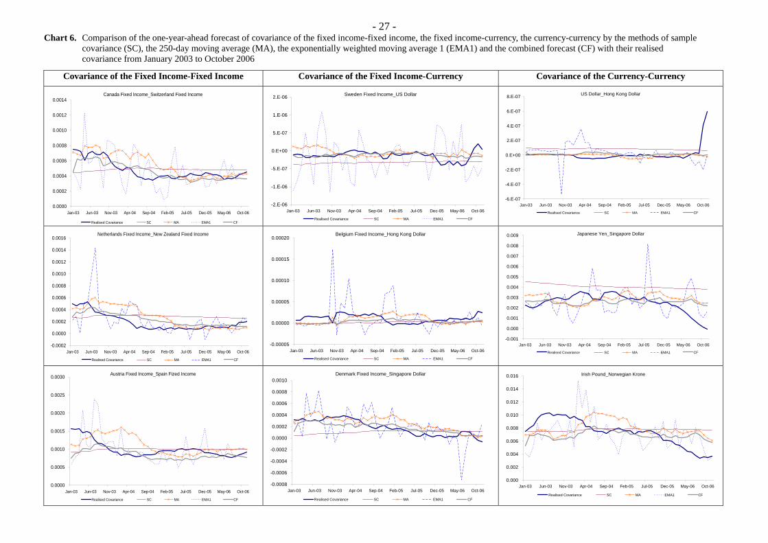
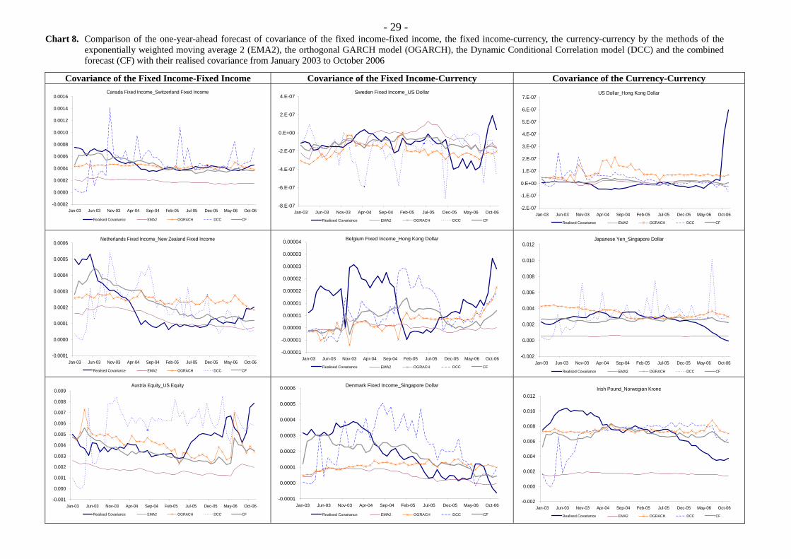
The observations in Charts 5 to 8 for the covariance matrix of the one-year ahead forecasts are similar to those in Charts 1 to 4. Same as the charts for the one-quarter ahead forecast, the realised covariance and the forecast from the CF method are plotted in all charts for comparison. The CF method tracks the mean level of the realised covariance well without large fluctuations. The EMA1 method, in Charts 5 and 6, and the DCC model, in Charts 7 and 8, give forecasts with peaks and troughs, which, however, do not match with those observed in the realised covariance. These non-synchronisations affect the overall performances of the EMA1 method and DCC model.

- 26 - Chart 5. Comparison of the one-year ahead forecast of covariance of the equity-equity, the equity-fixed income, the equity-currency by the methods of sample covariance (SC),

the 250-day moving average (MA), the exponentially weighted moving average (EMA1) and the combined forecast (CF) with their realised covariance from January 2003 to October 2006

Covariance of the Equity-Equity Covariance of the Equity-Fixed Income Covariance of the Equity-Currency Austria Equity_US Equity

-0.004

-0.002

0.000

0.002

0.004

0.006

0.008

0.010

0.012

0.014

Jan-03 Jun-03 Nov-03 Apr-04 Sep-04 Feb-05 Jul-05 Dec-05 May-06 Oct-06


Japan Equity_Finland Fixed Income

-0.0020

-0.0015

-0.0010

-0.0005

0.0000

0.0005

0.0010



US Equity_US Dollar

-8.E-06

-6.E-06

-4.E-06

-2.E-06

0.E+00

2.E-06

4.E-06

6.E-06

8.E-06



Australia Equity_Portugal Equity

-0.002

0.000

0.002

0.004

0.006

0.008

0.010

0.012



Portugal Equity_Japan Fixed Income

-0.0020

-0.0015

-0.0010

-0.0005

0.0000

0.0005

0.0010

0.0015

0.0020



Canada Equity_Hong Kong Dollar

-0.0004

-0.0002

0.0000

0.0002

0.0004

0.0006

0.0008


Realised Covariance SC MA EMA1 CF Hong Kong Equity_New Zealand Equity

-0.005

0.000

0.005

0.010

0.015

0.020



US Equity_Norway Fixed Income

-0.004

-0.003

-0.002

-0.001

0.000

0.001

0.002



Porgutal Equity_Norwegian Krone

-0.008

-0.006

-0.004

-0.002

0.000

0.002

0.004



- 27 - Chart 6. Comparison of the one-year-ahead forecast of covariance of the fixed income-fixed income, the fixed income-currency, the currency-currency by the methods of sample

covariance (SC), the 250-day moving average (MA), the exponentially weighted moving average 1 (EMA1) and the combined forecast (CF) with their realised covariance from January 2003 to October 2006

Covariance of the Fixed Income-Fixed Income Covariance of the Fixed Income-Currency Covariance of the Currency-Currency

Canada Fixed Income_Switzerland Fixed Income

0.0000

0.0002

0.0004

0.0006

0.0008

0.0010

0.0012

0.0014



Sweden Fixed Income_US Dollar

-2.E-06

-1.E-06

-5.E-07

0.E+00

5.E-07

1.E-06

2.E-06




-6.E-07

-4.E-07

-2.E-07

0.E+00

2.E-07

4.E-07

6.E-07

8.E-07


Realised Covariance SC MA EMA1 CF Netherlands Fixed Income_New Zealand Fixed Income

-0.0002

0.0000

0.0002

0.0004

0.0006

0.0008

0.0010

0.0012

0.0014

0.0016



Belgium Fixed Income_Hong Kong Dollar

-0.00005

0.00000

0.00005

0.00010

0.00015

0.00020



Japanese Yen_Singapore Dollar

-0.001

0.000

0.001

0.002

0.003

0.004

0.005

0.006

0.007

0.008

0.009


Realised Covariance SC MA EMA1 CF Austria Fixed Income_Spain Fized Income

0.0000

0.0005

0.0010

0.0015

0.0020

0.0025

0.0030



Denmark Fixed Income_Singapore Dollar

-0.0008

-0.0006

-0.0004

-0.0002

0.0000

0.0002

0.0004

0.0006

0.0008

0.0010



Irish Pound_Norwegian Krone

0.000

0.002

0.004

0.006

0.008

0.010

0.012

0.014

0.016



- 28 - Chart 7. Comparison of the one-year-ahead forecast of covariance of the equity-equity, the equity-fixed income, the equity-currency by the methods of the exponentially weighted

moving average 2 (EMA2), the orthogonal GARCH model (OGARCH), the Dynamic Conditional Correlation model (DCC) and the combined forecast (CF) with their realised covariance from January 2003 to October 2006

Covariance of the Equity-Equity Covariance of the Equity-Fixed Income Covariance of the Equity-Currency

Australia Equity_US Equity

-0.001

0.000

0.001

0.002

0.003

0.004

0.005

0.006

0.007

0.008

0.009


Realised Covariance EMA2 OGRACH DCC CF

Japan Equity_Finland Fixed Income

-0.0014

-0.0012

-0.0010

-0.0008

-0.0006

-0.0004

-0.0002

0.0000

0.0002



US Equity_US Dollar

-3.E-06

-2.E-06

-1.E-06

0.E+00

1.E-06

2.E-06

3.E-06

4.E-06

Jan-03 Jun-03 Nov-03 Apr-04 Sep-04 Feb-05 Jul-05 Dec-05 May-06 Oct-06Realised Covariance EMA2 OGRACH DCC CF

Australia Equity_Portugal Equity

0.000

0.001

0.002

0.003

0.004

0.005

0.006

0.007

0.008

0.009



Portugal Equity_Japan Fixed Income

-0.0009

-0.0008

-0.0007

-0.0006

-0.0005

-0.0004

-0.0003

-0.0002

-0.0001

0.0000

0.0001

0.0002

Jan-03 Jun-03 Nov-03 Apr-04 Sep-04 Feb-05 Jul-05 Dec-05 May-06 Oct-06Realised Covariance EMA2 OGRACH DCC CF

Canada Equity_Hong Kong Dollar

-0.00004

-0.00002

0.00000

0.00002

0.00004

0.00006

0.00008

0.00010


Realised Covariance EMA2 OGRACH DCC CF Hong Kong Equity_New Zealand Equity

0.000

0.002

0.004

0.006

0.008

0.010

0.012

0.014

0.016

0.018



US Equity_Norway Fixed Income

-0.0020

-0.0015

-0.0010

-0.0005

0.0000

0.0005



Porgutal Equity_Norwegian Krone

-0.004

-0.003

-0.002

-0.001

0.000

0.001

0.002

0.003



- 29 - Chart 8. Comparison of the one-year-ahead forecast of covariance of the fixed income-fixed income, the fixed income-currency, the currency-currency by the methods of the

exponentially weighted moving average 2 (EMA2), the orthogonal GARCH model (OGARCH), the Dynamic Conditional Correlation model (DCC) and the combined forecast (CF) with their realised covariance from January 2003 to October 2006

Covariance of the Fixed Income-Fixed Income Covariance of the Fixed Income-Currency Covariance of the Currency-Currency Canada Fixed Income_Switzerland Fixed Income

-0.0002

0.0000

0.0002

0.0004

0.0006

0.0008

0.0010

0.0012

0.0014

0.0016



Sweden Fixed Income_US Dollar

-8.E-07

-6.E-07

-4.E-07

-2.E-07

0.E+00

2.E-07

4.E-07




-2.E-07

-1.E-07

0.E+00

1.E-07

2.E-07

3.E-07

4.E-07

5.E-07

6.E-07

7.E-07


Realised Covariance EMA2 OGRACH DCC CF Netherlands Fixed Income_New Zealand Fixed Income

-0.0001

0.0000

0.0001

0.0002

0.0003

0.0004

0.0005

0.0006



Belgium Fixed Income_Hong Kong Dollar

-0.00001

-0.00001

0.00000

0.00001

0.00001

0.00002

0.00002

0.00003

0.00003

0.00004



Japanese Yen_Singapore Dollar

-0.002

0.000

0.002

0.004

0.006

0.008

0.010

0.012



Austria Equity_US Equity

-0.001

0.000

0.001

0.002

0.003

0.004

0.005

0.006

0.007

0.008

0.009



Denmark Fixed Income_Singapore Dollar

-0.0001

0.0000

0.0001

0.0002

0.0003

0.0004

0.0005

0.0006



Irish Pound_Norwegian Krone

-0.002

0.000

0.002

0.004

0.006

0.008

0.010

0.012



- 30 -

VII. CONCLUSION Modelling and forecasting the variance and covariance of returns are crucial in portfolio management and asset allocation. The variance and covariance of a portfolio are also essential to identify the overall risk of the portfolio as well as the risk of an individual asset. In recent years, there are advances in the methods of estimating and forecasting the covariance matrix in the literature, in particular for a large dimensional portfolio of assets. This paper examines and compares different methods which are recently proposed in the literature or widely used by the market practitioners.

Using a portfolio of 63 assets covering stocks, bonds and currencies from January 1998 to October 2007, the study finds that the CF method has consistently delivered the best performance among the seven methods. In fact, the outperformance of the combined forecast is more apparent in a longer forecast horizon (one-year ahead) than a shorter one (one-quarter ahead).

Despite the attractiveness of the combined forecasts shown in this study, it should be stressed that forecasting covariance of asset returns is still a daunting task. The forecast of volatility and covariance of asset returns from the combined forecast or any of these methods should be used with caution.

- 31 -

REFERENCES Alexander, C.O. (2001): “Orthogonal GARCH”, In: Alexander, C.O.(eds.) Mastering Risk Volume II, pp.21-38, Financial Times Prentice Hall, London. Alexander, C.O., Chibumba, A.M. (1997): “Multivariate orthogonal factor GARCH”, Mimeo, University of Sussex. Andersen, T.G., Bollerslev, T., Diebold, F.X., Labys, P. (2003): “Modeling and forecasting realized volatility”, Econometrica, 71, 529-626. Andersen, T.G., Bollerslev, T., Diebold, F.X., Wu, G. (2005): “A framework for exploring the macroeconomic determinants of systematic risk”, American Economic Review, 95, 398-404. Andersen, T.G., Benzoni, L. (2008): “Realized volatility”, SSRN. Available at http://ssrn.com/abstract=1092203. Bandi, F., Russel, J.R., Zhu, J. (2008): “Using high-frequency data in dynamic portfolio choice”, Econometric Reviews, 27, 163-198. Bates, J.M., Granger, C.W.J. (1969): “The combination of forecasts”, Operations Research Quarterly, 20, 451-68. Black, F. and Litterman, R. (1991): “Global asset allocation with equities, bonds, and currencies”, Available at http://www.hss.caltech.edu/media/from-carthage/filer/262.pdf Bollerslev, T., Zhang, B.Y.B. (2003): “Measuring and modeling systemic risk in factor pricing models using high-frequency data”, Journal of Empirical Finance, 10, 533-558. Byström, H.N.E. (2004): “Orthogonal GARCH and covariance matrix forecasting – The Nordic stock markets during the Asian financial crisis 1997-1998”, The European Journal of Finance, 10, 44-67. Diebold, F.X., Mariano, R. (1995): “Comparing predictive accuracy”, Journal of Business and Economic Statistics, 13, 253-263. Ding, Z. (1994): “Time Series Analysis of Speculative Returns”, PhD Thesis, UCSD. Ederington, L.H., Guan, W. (2004): “Forecasting volatility”, SSRN. Available at http://ssrn.com/abstract=165528. Engle, R.F. (2002): “Dynamic conditional correlation – A simple class of multivariate generalized autoregressive conditional heteroskedasticity models”, Journal of Business and Economic Statistics, 20, 339-350. Engle, R.F., Sheppard, K. (2001): “Theoretical and empirical properties of dynamic conditional correlation multivariate GARCH”, SSRN. Available at http://ssrn.com/abstract=287751.

- 32 -

Engle, R.F., Shephard, N., Shephard, K. (2008): “Fitting and testing vast dimensional time-varying covariance models”, SSRN. Available at http://ssrn.com/abstract=1293629. Fleming, J., Kirby, C., Ostdiek, B. (2003): “The economic value of volatility timing using realized volatility”. Journal of Financial Economics, 67, 473-509. J.P. Morgan (1996): “RiskMetrics – Technical Document”, J.P. Morgan. Litterman, R. and Winkelmann, K. (1998): “Estimating covariance matrices”, Available at http://citeseerx.ist.psu.edu/viewdoc/summary?doi=10.1.1.42.9221. Voev, V. (2008): “Dynamic modelling of large dimensional covariance matrices”, In: Bauwens, L., Pohlmeier, W., Veredas, D. (eds.) High Frequency Financial Econometrics, pp.293-312, Springer, Heidelberg. Wong, A.S.K., Vlaar, P.J.G. (2003): “Modelling time-varying correlations of financial markets”, Research Memorandum WO&E no.739. De Nederlansche Bank.

forecasting a large dimensional covariance matrix of a

Documents