form drag of subaqueous dune configurations
TRANSCRIPT

Master Thesis
Form drag of subaqueous dune configurations
Manfred JellesmaBSc., Civil Engineering (University of Twente, Enschede)
University of Twente & HKV LIJN IN WATERNovember 25, 2013
Under supervision of the master thesis committee:
Prof. dr. S.J.M.H. HulscherUniversity of Twente, Department of Water Engineering and Management
Dr. J.J. WarminkUniversity of Twente, Department of Water Engineering and Management
Dr. ir. A.J. PaarlbergHKV Consultants, Advisor rivers and coasts
Dr. A. LefebvreMARUM, Center for Marine Environmental Sciences
Dr. ir. G.H. KeetelsDelft University of Technology, Department of Maritime and Transport Technology

2

3
Preface
This master thesis presents the results of a study to the form drag of subaqueous duneconfigurations in rivers. The research is carried out in cooperation with the University ofTwente and HKV Consultants.
I would like to thank all my committee members for helping me out in the past six months.First of all I have to thank Andries Paarlberg for his guiding and support on a daily basisduring the research at HKV Consultants. You always had time for my daily problemsand helped me out with some out of the box thoughts. Secondly I have to thank AliceLefebvre for sharing her knowledge and results on dune modelling in Delft3D. Thanks foryour supporting and always encouraging e-mails. From the University of Twente I thankJord J. Warmink and Suzanne J.M.H. Hulscher for their guidance during the preparationsof the master thesis and for giving critical reviews and structure to the research later on.The last committee members I have to thank is Geert H. Keetels. I really appreciatedyour unconditional help on OpenFOAM, although you joined the committee later.
Other than my committee, I have to thank my unofficial committee member, FredrikHuthoff as well for his guiding and support at HKV Consultants. Thanks for learning methe basics and some useful features of OpenFOAM. Finally I want to show my gratitude toHKV Consultants for giving me the opportunity to conduct this research and facilitatingthe working environment.

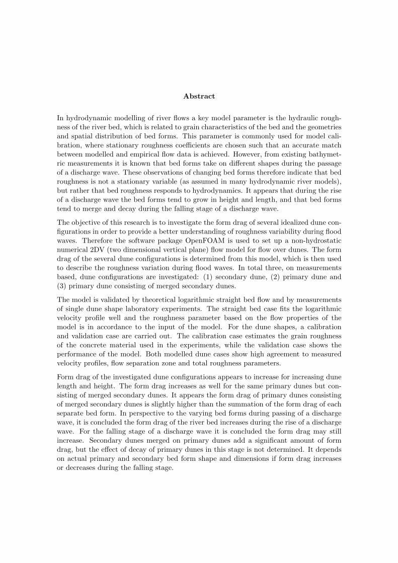
Abstract
In hydrodynamic modelling of river flows a key model parameter is the hydraulic rough-ness of the river bed, which is related to grain characteristics of the bed and the geometriesand spatial distribution of bed forms. This parameter is commonly used for model cali-bration, where stationary roughness coefficients are chosen such that an accurate matchbetween modelled and empirical flow data is achieved. However, from existing bathymet-ric measurements it is known that bed forms take on different shapes during the passageof a discharge wave. These observations of changing bed forms therefore indicate that bedroughness is not a stationary variable (as assumed in many hydrodynamic river models),but rather that bed roughness responds to hydrodynamics. It appears that during the riseof a discharge wave the bed forms tend to grow in height and length, and that bed formstend to merge and decay during the falling stage of a discharge wave.
The objective of this research is to investigate the form drag of several idealized dune con-figurations in order to provide a better understanding of roughness variability during floodwaves. Therefore the software package OpenFOAM is used to set up a non-hydrostaticnumerical 2DV (two dimensional vertical plane) flow model for flow over dunes. The formdrag of the several dune configurations is determined from this model, which is then usedto describe the roughness variation during flood waves. In total three, on measurementsbased, dune configurations are investigated: (1) secondary dune, (2) primary dune and(3) primary dune consisting of merged secondary dunes.
The model is validated by theoretical logarithmic straight bed flow and by measurementsof single dune shape laboratory experiments. The straight bed case fits the logarithmicvelocity profile well and the roughness parameter based on the flow properties of themodel is in accordance to the input of the model. For the dune shapes, a calibrationand validation case are carried out. The calibration case estimates the grain roughnessof the concrete material used in the experiments, while the validation case shows theperformance of the model. Both modelled dune cases show high agreement to measuredvelocity profiles, flow separation zone and total roughness parameters.
Form drag of the investigated dune configurations appears to increase for increasing dunelength and height. The form drag increases as well for the same primary dunes but con-sisting of merged secondary dunes. It appears the form drag of primary dunes consistingof merged secondary dunes is slightly higher than the summation of the form drag of eachseparate bed form. In perspective to the varying bed forms during passing of a dischargewave, it is concluded the form drag of the river bed increases during the rise of a dischargewave. For the falling stage of a discharge wave it is concluded the form drag may stillincrease. Secondary dunes merged on primary dunes add a significant amount of formdrag, but the effect of decay of primary dunes in this stage is not determined. It dependson actual primary and secondary bed form shape and dimensions if form drag increasesor decreases during the falling stage.


Contents
Preface . . . . . . . . . . . . . . . . . . . . . . . . . . . . . . . . . . . . . . 3
1 Introduction 11
1.1 River bed forms . . . . . . . . . . . . . . . . . . . . . . . . . . . . . . . . . . 11
1.2 River bed roughness . . . . . . . . . . . . . . . . . . . . . . . . . . . . . . . 12
1.2.1 Grain roughness . . . . . . . . . . . . . . . . . . . . . . . . . . . . . 12
1.2.2 Form drag . . . . . . . . . . . . . . . . . . . . . . . . . . . . . . . . . 14
1.2.3 Turbulent kinetic energy . . . . . . . . . . . . . . . . . . . . . . . . . 15
1.3 Research objective . . . . . . . . . . . . . . . . . . . . . . . . . . . . . . . . 16
1.3.1 Research questions . . . . . . . . . . . . . . . . . . . . . . . . . . . . 16
1.3.2 Structure of the report . . . . . . . . . . . . . . . . . . . . . . . . . . 16
2 Methods 19
2.1 Set up of the model . . . . . . . . . . . . . . . . . . . . . . . . . . . . . . . 19
2.1.1 OpenFOAM . . . . . . . . . . . . . . . . . . . . . . . . . . . . . . . . 19
2.1.2 Boundary conditions . . . . . . . . . . . . . . . . . . . . . . . . . . . 19
2.1.3 Adapted interFoam solver . . . . . . . . . . . . . . . . . . . . . . . . 21
2.1.4 Turbulence model . . . . . . . . . . . . . . . . . . . . . . . . . . . . 22
2.1.5 Grain roughness implementation . . . . . . . . . . . . . . . . . . . . 22
2.1.6 Construction of the mesh . . . . . . . . . . . . . . . . . . . . . . . . 23
2.2 Flow conditions . . . . . . . . . . . . . . . . . . . . . . . . . . . . . . . . . . 25
2.3 Roughness determination . . . . . . . . . . . . . . . . . . . . . . . . . . . . 25
2.3.1 Total roughness . . . . . . . . . . . . . . . . . . . . . . . . . . . . . . 26
2.3.2 Grain roughness . . . . . . . . . . . . . . . . . . . . . . . . . . . . . 26
3

4 CONTENTS
3 Model calibration and validation 27
3.1 Flat bed validation . . . . . . . . . . . . . . . . . . . . . . . . . . . . . . . . 27
3.1.1 Model results . . . . . . . . . . . . . . . . . . . . . . . . . . . . . . . 28
3.1.2 Sensitivity analysis . . . . . . . . . . . . . . . . . . . . . . . . . . . . 30
3.2 Dune calibration and validation . . . . . . . . . . . . . . . . . . . . . . . . . 31
3.2.1 ML2 and ML6 mesh . . . . . . . . . . . . . . . . . . . . . . . . . . . 32
3.2.2 Calibration results ML2 . . . . . . . . . . . . . . . . . . . . . . . . . 33
3.2.3 Validation results ML6 . . . . . . . . . . . . . . . . . . . . . . . . . . 36
3.2.4 Mesh sensitivity . . . . . . . . . . . . . . . . . . . . . . . . . . . . . 37
4 Model experiments 41
4.1 Dune configurations . . . . . . . . . . . . . . . . . . . . . . . . . . . . . . . 41
4.2 Model settings . . . . . . . . . . . . . . . . . . . . . . . . . . . . . . . . . . 43
4.3 Model output . . . . . . . . . . . . . . . . . . . . . . . . . . . . . . . . . . . 44
4.3.1 Case 0 - Flat bed . . . . . . . . . . . . . . . . . . . . . . . . . . . . . 45
4.3.2 Case 1 - Secondary dune . . . . . . . . . . . . . . . . . . . . . . . . . 46
4.3.3 Case 2 - Primary dune . . . . . . . . . . . . . . . . . . . . . . . . . . 47
4.3.4 Case 3 - Primary dune and secondary dunes . . . . . . . . . . . . . . 48
4.4 Form drag of the experimental dune configurations . . . . . . . . . . . . . . 49
5 Discussion 51
5.1 Roughness variability during flood waves . . . . . . . . . . . . . . . . . . . . 51
5.1.1 Form drag of bed form evolution stage 1, 2 and 3 . . . . . . . . . . . 51
5.1.2 Form drag of bed form evolution stage 4, 5 and 6 . . . . . . . . . . . 52
5.2 Model assumptions . . . . . . . . . . . . . . . . . . . . . . . . . . . . . . . . 53
5.2.1 Laboratory scale versus field scale . . . . . . . . . . . . . . . . . . . 53
5.2.2 Static and idealized shaped bed forms . . . . . . . . . . . . . . . . . 55
5.2.3 2DV model versus 3D reality . . . . . . . . . . . . . . . . . . . . . . 55
5.3 Improvements of the model set up . . . . . . . . . . . . . . . . . . . . . . . 56
6 Conclusions and outlook 57
6.1 Conclusions . . . . . . . . . . . . . . . . . . . . . . . . . . . . . . . . . . . . 57
6.2 Outlook . . . . . . . . . . . . . . . . . . . . . . . . . . . . . . . . . . . . . . 58
A Technical details boundary conditions 63

CONTENTS 5
B Adapted interFoam solver 64
C Convergence of the solutions generated by the free surface OpenFOAMmodel 65
D Sensitivity analysis flat bed case 66
E Dune validation cases including Delft3D results 69
F Constructed meshes for model experiments 74
G Sensitivity varying grain roughness 77

6 CONTENTS

List of Figures
1.1 Properties of subaqueous dunes . . . . . . . . . . . . . . . . . . . . . . . . . 12
1.2 Proposed model of bed form evolution under varying discharge in flume andfield (Warmink et al., 2012) . . . . . . . . . . . . . . . . . . . . . . . . . . . 13
1.3 Flow regions for a turbulent flow over a straight bed . . . . . . . . . . . . . 14
1.4 Schematic representation of the flow regions in flow over dunes (Best, 2005) 15
2.1 Schematic model setup (flat bed case) . . . . . . . . . . . . . . . . . . . . . 20
2.2 Schematic model setup (dune case) . . . . . . . . . . . . . . . . . . . . . . . 20
3.1 Mesh and dimensions of the flat bed validation (Flat bed 1a) . . . . . . . . 29
3.2 Theoretical versus modelled velocity profile (flat bed case 1a) . . . . . . . . 29
3.3 Velocity profiles of all flat bed cases . . . . . . . . . . . . . . . . . . . . . . 31
3.4 Mesh created for ML2 dune validation . . . . . . . . . . . . . . . . . . . . . 33
3.5 Mesh created for ML6 dune validation . . . . . . . . . . . . . . . . . . . . . 33
3.6 ML2 - Velocity profiles of measurements of McLean (black) and modelledby OpenFOAM (red). Velocities are scaled by a factor 10. . . . . . . . . . . 35
3.7 ML2 - Flow separation zones of measurements of McLean (black dots) andOpenFOAM (red line) . . . . . . . . . . . . . . . . . . . . . . . . . . . . . . 36
3.8 ML6 - Velocity profiles of measurements of McLean (black) and modelledby OpenFOAM (red). Velocities are scaled by a factor 20. . . . . . . . . . . 38
3.9 ML6 - Flow separation zones of measurements of McLean (black dots) andOpenFOAM (red line) . . . . . . . . . . . . . . . . . . . . . . . . . . . . . . 39
4.1 Measured dune dimensions (Julien et al. (2002); Wilbers and Ten Brinke(2003)) and experimental or hypothetical dune shape properties (McLeanet al. (1999a); Ogink (1989); Warmink et al. (2012)) . . . . . . . . . . . . . 41
4.2 Dune case 1: Secondary dune . . . . . . . . . . . . . . . . . . . . . . . . . . 42
4.3 Dune case 2: Primary dune . . . . . . . . . . . . . . . . . . . . . . . . . . . 43
4.4 Dune case 3: Primary dune containing secondary dunes . . . . . . . . . . . 43
7

8 LIST OF FIGURES
4.5 Case 0 - Flat bed: Horizontal velocities and streamlines . . . . . . . . . . . 45
4.6 Case 0 - Flat bed: Turbulent kinetic energy . . . . . . . . . . . . . . . . . . 45
4.7 Case 1 - Secondary dune: Horizontal velocities and streamlines . . . . . . . 46
4.8 Case 1 - Secondary dune: Turbulent kinetic energy . . . . . . . . . . . . . . 47
4.9 Case 2 - Primary dune: Horizontal velocities and streamlines . . . . . . . . 48
4.10 Case 2 - Primary dune: Turbulent kinetic energy . . . . . . . . . . . . . . . 48
4.11 Case 3 - Primary dune containing secondary dunes: Horizontal velocitiesand streamlines . . . . . . . . . . . . . . . . . . . . . . . . . . . . . . . . . . 49
4.12 Case 3 - Primary dune containing secondary dunes: Turbulent kinetic energy 49
4.13 Total Nikuradse roughness of the three dune cases and the flat bed case . . 50
B.1 Adapated UEqn.h file of the interFoam solver . . . . . . . . . . . . . . . . . 64
C.1 Residuals and Courant numbers of the flat bed validation . . . . . . . . . . 65
D.1 Mesh used for flatbed 1a, 1b and 1c (varying roughness constant cs) . . . . 66
D.2 Mesh used for flatbed 2 (surface refinement) . . . . . . . . . . . . . . . . . . 67
D.3 Mesh used for flatbed 3 (total refinement) . . . . . . . . . . . . . . . . . . . 67
D.4 Mesh used for flatbed 4a (bottom refinement using SnappyHexMesh) . . . . 68
D.5 Mesh used for flatbed 4b (partly bottom refinement using SnappyHexMesh) 68
E.1 ML2 - Velocity profiles of measurements of McLean (black), modelled byDelft3D (blue) and modelled by OpenFOAM (red). Velocities are scaled bya factor 1
10 . . . . . . . . . . . . . . . . . . . . . . . . . . . . . . . . . . . . . 70
E.2 ML2 - Flow separation zones of measurements of McLean (black dots),Delft3D (blue dots) and OpenFOAM (red line) . . . . . . . . . . . . . . . . 71
E.3 ML6 - Velocity profiles of measurements of McLean (black), modelled byDelft3D (blue) and modelled by OpenFOAM (red). Velocities are scaled bya factor 1
10 . . . . . . . . . . . . . . . . . . . . . . . . . . . . . . . . . . . . . 72
E.4 ML6 - Flow separation zones of measurements of McLean (black dots),Delft3D (blue dots) and OpenFOAM (red line) . . . . . . . . . . . . . . . . 73
F.1 Flatbed: Mesh . . . . . . . . . . . . . . . . . . . . . . . . . . . . . . . . . . 74
F.2 Case 1 - Secondary dune: Mesh . . . . . . . . . . . . . . . . . . . . . . . . . 75
F.3 Case 2 - Primary dune: Mesh . . . . . . . . . . . . . . . . . . . . . . . . . . 75
F.4 Case 3 - Primary dune: Mesh . . . . . . . . . . . . . . . . . . . . . . . . . . 76

List of Tables
3.1 Specified roughness (input) compared to the roughness based on the averagevelocity of the logarithmic and modelled velocity profile (flat bed case 1a) . 30
3.2 Sensitivity in grain roughness output parameters . . . . . . . . . . . . . . . 31
3.3 ML2 - Calibration of z0 grain roughness parameter . . . . . . . . . . . . . . 34
3.4 ML6 - Validation of flow velocities and total roughness . . . . . . . . . . . . 36
4.1 Nikuradse form drag of the experimental dune configurations . . . . . . . . 50
5.1 Scaling of dune configuration case 3 to field scale conditions . . . . . . . . . 54
5.2 Comparison of scaled roughness of the dune configurations and the rough-ness estimation based on equation 5.1 . . . . . . . . . . . . . . . . . . . . . 54
A.1 Technical details of the used boundary conditions in the OpenFOAM model 63
C.1 Residuals and Courant numbers of the dune validation and model experiments 65
G.1 Sensitivity of the average velocity, total roughness and form roughness incomparison to the variation of the grain roughness . . . . . . . . . . . . . . 78
9

10 LIST OF TABLES

Chapter 1
Introduction
In The Netherlands the flood defence system of rivers is based on the occurring water levelsduring a certain high discharge event. This high discharge event, the design discharge, iscoupled to a very low chance of occurrence following the Dutch regulation. Since no fielddata are available of such rare events, existing discharge measurements are extrapolatedin order to find the discharge given a certain chance. The design water levels follow fromnumeric models, using this design discharge as boundary condition.
In numeric models the discharge wave, river dimensions and roughness of the bed are thekey parameters controlling the water levels. While the discharge wave and river dimensionscan be reasonably estimated, much is yet unknown about the bed roughness in rivers.Therefore, the bed roughness parameters are often used to calibrate the models usingfixed roughness parameters in time.
However, several researchers (e.g. Julien et al. (2002); Wilbers and Ten Brinke (2003))indicate that the bed roughness parameters are likely to change with varying discharge.The changing flow conditions during a discharge wave (flow velocities and water depth)influence the sediment transport at the river bed and therefore cause for different bedforms to occur. It is likely that these bed forms cause the river bed roughness to change,which is in contradiction to the fixed roughness parameters used in the numerical modelsfor the prediction of water levels.
This chapter explains the main characteristics of bed forms, river bed roughness anddefines the research objective of this research.
1.1 River bed forms
River bed forms develop due to the interaction between flow and a moveable bed. For aflow over an initial plane bed, if sediment transport occurs, the bed may become unstableand bed forms start to develop (Engelund, 1967). Dunes are typical bed forms arising atthe river bed. Dunes occur in different dimensions and shapes which all mainly dependon water depth, flow velocity and sediment properties. For this research the shape of thedunes is assumed to be asymmetrical. Typical asymmetrical dunes consist of a gentle stossside and a relatively steep lee side (figure 1.1). Other important dune properties are thedune length and the crest height.
11

12 CHAPTER 1. INTRODUCTION
Figure 1.1: Properties of subaqueous dunes
Assuming the sediment properties do not change during a discharge event, the dune dimen-sions mainly depend on water depth and flow velocity. Under, steady conditions, erosiontowards the crest equals deposition just after the crest and dune dimensions are in equilib-rium. Dunes then migrate in the direction of the flow (for Froude numbers smaller than 1)(Knighton, 1998). However, in most rivers discharge is constantly changing and thereforeno equilibrium situation is reached. In fact, due the slow morphological processes, the bedis in constant movement towards a new equilibrium situation.
Warmink et al. (2012) stated different hypothetical stages of bed forms during a dischargewave, which are believed to show a general pattern of bed forms during discharge wavesin rivers (figure 1.2). In these stages a hysteresis in bed forms and discharge is clearlyvisible (also observed by Julien et al. (2002); Wilbers and Ten Brinke (2003)). During lowdischarge dunes are small, but they grow larger with increasing discharge. When the peakdischarge has passed, dunes continue to grow due to the lagged adaptation of sedimentprocesses to flow properties. At the end of the discharge wave the dunes become lowerand smoother (lower angles) but keep increasing in length. In this phase smaller dunes(secondary dunes) start to arise on top of these dunes.
1.2 River bed roughness
The roughness of a river depends on all of the induced resistances to the flow. The flowresistance is for example influenced by vegetation, bed material, bed shape or structures(groynes, bridges). However, in theoretical research the roughness of rivers is assumed toconsist of only bed roughness. Bed roughness is the total roughness to the flow inducedby the river bottom. The roughness of the banks of a river are often neglected, which isappropriate when dealing with relatively wide rivers. The total river roughness is for thisresearch assumed to consist of only the bed roughness. The two main components of bedroughness consists of grain friction 1 and form drag 2 (e.g. Ogink (1989); Julien et al.(2002)).
1.2.1 Grain roughness
Grain roughness refers to resistance to flow due to the shear stress applied on individualgrains on the river bed (Julien et al., 2002). For a turbulent flow subjected only to grain
1Grain roughness results from resistance to flow due to the shear stress applied on individual grains.2Form drag results from pressure gradients in the flow which induces turbulence and leads to energy
dissipation.

1.2. RIVER BED ROUGHNESS 13
Figure 1.2: Proposed model of bed form evolution under varying discharge in flume andfield (Warmink et al., 2012)
roughness the velocities are theoretically approximated by a logarithmic velocity profile(van Rijn, 1993) for which several regions are distinguished (figure 1.3). The viscous sub-layer is a very small laminar layer close to the wall where viscous shear stresses dominate(Booij, 1992) and the velocities at the wall are usually assumed to be zero (Knighton,1998). In this region the velocity gradient is approximately linear (Booij, 1992). Thebuffer region is a transition layer from laminar to turbulent flow where both the viscousand turbulent stresses are important (Booij, 1992). In the fully turbulent region turbulent

14 CHAPTER 1. INTRODUCTION
stresses dominate (Booij, 1992) and velocity varies semi-logarithmically with the waterdepth (Knighton, 1998). This layer extends over 10 to 20 per cent of the water depth.The upper 80 to 90 per cent consists of the outer layer, where large scale turbulence ispresent and the velocity profile diverges from a semi-logarithmic form (Knighton, 1998).
Figure 1.3: Flow regions for a turbulent flow over a straight bed
Grain roughness properties of the bed can be expressed by the Nikuradse roughness lengthks and roughness height z0. Expression of the Nikuradse roughness length into roughnessheight depends on the roughness regime. The dimensions of grain particles at the riverbed often exceed the height of the viscous sublayer and the flow regime is hydraulicallyrough. For flows where the grain particles of the bed do not exceed the size of the viscoussublayer the flow is defined as hydraulically smooth. The mathematical definition of thehydraulically rough and smooth regime are given by equation 1.1 and 1.2 (van Rijn, 1993):
ksu∗ν
>> 1 (1.1)
ksu∗ν
<< 1 (1.2)
ks = Nikuradse roughness [m]
u∗ = shear velocity [m/s]
ν = kinematic viscosity [m2/s]
For this research all flow regimes meet the hydraulically rough condition.
1.2.2 Form drag
The flow over an asymmetric dune separates at the crest, creating a large separation zonein the trough. According to Paarlberg et al. (2007) the main turbulence pattern behind adune consists of a circular flow, called the flow separation zone, which is most influencedby the dune height and the angle at the flow separation point. The difference in pressurebetween the stoss and lee sides produces a net force on the dune called form drag (Madduxet al., 2003).
Best (2005) summarized five major regions in flow over river dunes. These region apply toasymmetrical dunes with an angle-of-repose lee side and are generated in a steady, uniformunidirectional flow.

1.2. RIVER BED ROUGHNESS 15
Regions in flow over asymmetrical dunes:
1. A region of flow separation is formed in the lee of the dune
2. A shear layer is generated bounding the separation zone
3. A third region is one of expanding flow in the dune lee side
4. New internal boundary layer grows as flow re-establishes itself
5. Maximum horizontal velocity profile occurs of the dunes crest
Figure 1.4: Schematic representation of the flow regions in flow over dunes (Best, 2005)
Figure 1.4 visualises flow separation at the crest and circular flow in the trough of thedune. Behind the flow separation zone a wake region arises, covering high turbulencesin the flow. The flow separation zone is therefore of high importance for the amount ofform drag. On the stoss side the flow recovers from turbulences and reaches maximumvelocities towards the crest.
1.2.3 Turbulent kinetic energy
The grain roughness and the form drag of the river bed both induce turbulences whichresults in resistance to the flow. The Turbulent Kinetic Energy (TKE) is defined by themean kinetic energy associated with these turbulences in the flow. Cross sectional plotsof the TKE are therefore useful for showing the location and intensity of turbulence. Inparticular for form drag the TKE reveals high turbulent regions in the water column, likethe wake region visualised in figure 1.4.

16 CHAPTER 1. INTRODUCTION
1.3 Research objective
The objective of this research is defined:
To provide a better understanding of the roughness variability during flood waves, bycomputing the form drag of typical primary and secondary dune configurations in rivers.
Typical occurring dune configurations refer to the 6 stages of the bed form evolutionprocess during a flood (chapter 1). By making use of 2DV (two dimensional verticalplane) numerical modelling, the flow over typical bedforms is simulated and the outputflow properties are used to derive the form drag.
The numerical modelling is conducted using the CFD (Computational Fluid Dynamics)software package OpenFOAM. OpenFOAM is open source, therefore free to use, andprovides the ability of constructing and computing ’flexible’ meshes. This means the meshcan be locally refined without increasing the mesh resolution of the whole domain.
1.3.1 Research questions
In order to give guidance to the research objective, the following research questions aredefined:
1. Which model settings are used for creating a free surface model in OpenFOAM?
2. How do the model results compare to a validation reference case?
3. What is the form drag of the investigated dune configurations?
4. What are the variations in form drag during floods, following the proposed model ofbed form evolution (figure 1.2)?
1.3.2 Structure of the report
A short overview of the structure of the report is given below:
• Chapter 1: IntroductionGeneral introduction to river bed forms, river bed roughness and definition of theresearch objective.
• Chapter 2: MethodsDescribes the free surface OpenFOAM model and the general model settings. Be-sides the general flow conditions and the method of form drag and grain roughnessdetermination is explained.
• Chapter 3: Model calibration and validationThe fundamentals of the free surface OpenFOAM model are validated by the log-arithmic velocity profile over a straight bed. Next, the model is calibrated andvalidated by measurements of laboratory experiments of flow over dunes.

1.3. RESEARCH OBJECTIVE 17
• Chapter 4: Model experimentsThree experimental dune configurations are defined and the resulting modelled flowover these bed forms is discussed.
• Chapter 5: DiscussionThe results of experimental dune configurations are discussed in perspective to vari-ations in form drag of the proposed dune evolution process. Besides the influence ofthe most important assumptions of the model and the bed forms is explained. Thelast part of this chapter proposes several recommendations for improvement of themodel set up.
• Chapter 6: Conclusions and recommendationsThe general conclusions of the research are summarized by answering the researchquestions. Besides several recommendations for future research are proposed.

18 CHAPTER 1. INTRODUCTION

Chapter 2
Methods
This chapter explains the model settings, flow conditions and method used for derivingthe form drag from flow properties.
2.1 Set up of the model
The main parts of the model are explained in this section. OpenFOAM is shortly intro-duced after which the boundary conditions, solver and turbulence model are discussed.The last part explains the grain roughness specification in the free surface model and theconstruction of the mesh.
2.1.1 OpenFOAM
OpenFOAM is a multi-dimensional open source CFD (Computation Fluid Dynamics)which has a wide range of standard solvers for different flow conditions. However, funda-mentally OpenFOAM is a tool for solving partial differential equations rather than a CFDpackage in the traditional sense. Therefore it can also be used in other areas like stressanalysis, electromagnetic and finance (OpenFOAM Foundation, 2013).
For the purpose of this research OpenFOAM is used to set up a 2DV (two dimensionalvertical plane) free surface flow by modelling both water and air particles.
2.1.2 Boundary conditions
Boundary conditions need to be chosen properly, since they are of high importance tothe model and have a high influence on model output. The boundary conditions for themodel are separated into hydraulic and spatial boundary conditions. Hydraulic boundaryconditions are boundaries applicable to water and air, while spatial boundary conditionsrefer to the spatial domain of the model.
Hydraulic boundary conditions
The inlet and outlet of the model consist of ’cyclic’ boundary conditions. This meansthat the flow and its properties that exit the model, enter the model at the inlet. The
19

20 CHAPTER 2. METHODS
advantage gained by using cyclic boundary conditions is that for repetitive bed forms themodel domain is kept small. The ceiling of the model, called ’atmosphere’, consists ofan ’inlet-outlet’ boundary condition. Therefore air is allowed to flow in or out at thisboundary. The bottom boundary condition is set to the type ’wall’. By specifying thebottom boundary as ’wall’, wall functions are applicable to this boundary and roughnesscan be specified. The utility of wall functions and the addition of a certain roughnessto the boundary is explained in section 2.1.6. More technical details of the boundaryconditions used in the model are found in appendix A. A schematic representation of themodel is shown in figure 2.1 and 2.2.
Figure 2.1: Schematic model setup (flat bed case)
Figure 2.2: Schematic model setup (dune case)
Spatial boundary conditions
Due the use of cyclic boundary conditions, the spatial domain of the model can be limitedto include one bed form (figure 2.2 illustrates this). Therefore the domain length dependson the length of the bed form. The model height depends on the water level and thethickness of the atmospheric layer above the water surface. In all cases the thickness ofthe atmospheric layer is modelled by 10 equally sized cells, which have the same dimensionsas cells just below the water surface.

2.1. SET UP OF THE MODEL 21
2.1.3 Adapted interFoam solver
OpenFOAM contains many solvers for different purposes. The interFoam solver is used inthis research, since the interFoam solver is able to model the behaviour of two incompress-ible fluids. In the context of hydraulic flow modelling, these two fluids consist of waterand air. The interest for this research lies in the modelling of water particles. However bymodelling the air particles as well, a free water surface is created.
The standard interFoam solver is not able to model a free surface flow using cyclic bound-ary conditions. To make the interFoam solver work properly with cyclic boundary condi-tions, the flow needs to be driven by a horizontal force.
The interFoam solver solves the Reynolds-Averaged Navier-Stokes (RANS) equations,which consist of the continuity equation (equation 2.1) and momentum equation (equation2.2) (Liu et al., 2008). In order to generate a horizontal forcing on the flow an extra term(ρ Bodyforce) on the right hand side is added to the momentum equation. The ’Body-force’ parameter defines the size and direction of a force. Therefore this force consistsof an x-, y- and z-component. For the purpose of 2DV free surface flow only a flow inx-direction is needed. The size of the force is defined by the gravitational force times thebed slope of the channel (equation 2.4).
∇ · u = 0 (2.1)
∂ρu
∂t+∇ · (ρu u)−∇ · ((µ+ µt)S) = −∇p+ ρg + σK
∇α| ∇α |
(2.2)
u = velocity vector field
∇ = divergence in the x−, y − and z − directionp = pressure field
µ = viscosity
µt = turbulent eddy viscosity
S = strain rate tensor
α = volume fraction (0 : air, 1 : water)
σ = surface tension
K = surface curvature
∂ρu
∂t+∇ · (ρu u)−∇ · ((µ+ µt)S) = −∇p+ ρg + σK
∇α| ∇α |
+ ρ Bodyforce (2.3)
Bodyforce = ( ig︸︷︷︸x−component
0︸︷︷︸y−component
0︸︷︷︸z−component
) (2.4)
The entire code of the adapted interFoam solver can be found in appendix B.

22 CHAPTER 2. METHODS
2.1.4 Turbulence model
OpenFOAM supports a wide range of turbulence models. In this research the conventionalk-epsilon turbulence model is used to simulate turbulence. In this model k defines turbu-lent kinetic energy, while ε expresses the turbulent energy dissipation rate. The k-epsilonturbulence model is a high Reynolds number turbulence model, which means the modelcan not solve the flow entirely to the wall (where the Reynolds number is low). Thereforewall functions are applied to the first cells at the wall boundaries, which give the abilityof applying a certain roughness to these walls. The values of the turbulence parameters ofthe k-epsilon model are not changed and have default values programmed in OpenFOAM:
Cµ = 0.09
C1 = 1.44
C2 = 1.92
σε = 1.3
In an earlier stage of this research also the k-ω SST turbulence model was applied. TheSST k-ω model is a combination of the k-epsilon model (for high Reynolds number mod-elling) and the k-ω model (for low Reynolds number modelling). This makes the SSTk-ω turbulence model suitable for modelling both laminar and turbulent regions of theflow (section 1.2.1). For this research however, the time to solve the flow entirely to thewall would take to much time in perspective to the improvement in accuracy. Thereforewall functions were applied, but during the model validation the k-epsilon model provedto model the flow separation zone more accurately. This is remarkable since both thek-epsilon and the k-ω SST model should perform alike in high turbulent zones. However,according to Moradnia (2010), not meeting the y+ requirements (section 2.1.6) in themodel results in impaired results for the k-omega SST model in contrast to the k-epsilonmodel. Some areas of the dune profile (close to the dune trough where flow velocities arelow) do not satisfy the y+ requirements during the dune validation, which may explainthe better performance of the k-epsilon model.
2.1.5 Grain roughness implementation
Due the use of the k-epsilon turbulence model the grain roughness of the bottom in themodel is applied by wall functions. The grain roughness is defined by two parameters,the roughness constant cs and the roughness height ks. The roughness height and theroughness constant together specify the z0 at the bottom according equation 2.5 (e.g.Pattanapol et al. (2007); Martinez (2011)). The equation shows that it is possible tospecify the same roughness z0 by different parameter values for cs and ks.
It may sometimes be useful to change the roughness constant cs in order to meet the ratiorequirement between the first cell height and the roughness described in section 2.1.6. Thevalue of cs may vary from 0.5 to 1.0 according to OpenFOAM Foundation (2012), however(Pattanapol et al., 2007) states that the same roughness implementation (2.5) is used forAnsys Fluent but the roughness constant is fixed to a value of 0.327. Sensitivity analysesfor the flat bed validation (section 3.1.2) show that the use of a roughness constant valueof 0.327, 0.5 or 1.0 makes no difference if the roughness height (z0) in those cases ismaintained. Except for these sensitivity analyses, all cases modelled in this research areconducted using a roughness constant value of 1.0.

2.1. SET UP OF THE MODEL 23
ks =E
cs∗ z0 (2.5)
ks = roughness height [m]
E = empirical parameter [−] = 9.793
cs = roughess constant [−]
z0 = roughness length [m]
2.1.6 Construction of the mesh
Creating an appropriate mesh is of high importance for both model output and calculationtime. Therefore a set of guidelines and restrictions are defined for creating a mesh. Theguidelines are based on the research of Lefebvre et al. (2013) and give guidance in theamount of grid cells needed in the flow separation zone and the water column. However, itshould be noticed the research of Lefebvre et al. (2013) is carried out in Delft3D (modellingone phase: water), while OpenFOAM (modelling two phases: water and air) is used forthis research. Therefore applying the same mesh settings may not necessarily lead to goodresults, but during the validation process it is found they fit for OpenFOAM as well. Therestrictions are related to the dimensions of the first cells adjacent to the bottom and areneeded in order to correctly model the grain roughness.
Guidelines
A set of guidelines are stated and used for building meshes for the dune cases. By us-ing these guidelines, time consuming sensitivity analyses for finding the optimum meshsettings are avoided. The risk taken by this approach is that the optimum mesh settingsfor OpenFOAM may require more or even less grid cells. However, the calibration andvalidation cases (chapter 3) show that using the guidelines give appropriate model resultsin comparison to measurements and the model has reasonable runtimes.
• Horizontal spacingEach dune profile is split into at least 100 profiles (equal distance). This is applied for both
primary and secondary dunes.
• Water columnThe area between the water surface and the crest of the dune should consists of 20 layers.
• Flow separation zoneThe vertical distance between de through and the crest of the dune are divided into 30 layers,
while another 5 layers are added just above the crest.
Restrictions for cells adjacent to the bottom
To correctly model grain roughness in the model two conditions have to be satisfied. Ingeneral these conditions apply to the height of the cells adjacent to a wall. For the freesurface model the bottom acts like a wall and the conditions apply to the first cells adjacentto the bottom.

24 CHAPTER 2. METHODS
y+ restrictionThe y+ value is a dimensionless height parameter which indicates in which region of theflow (section 1.2.1) cells adjacent to the wall are located. In section 2.1.4 it is explainedthat the k-epsilon turbulence is only able of solving the turbulent region of the flow.Therefore it needs to be avoided that the first cells adjacent to the wall are located in thesmall viscous sublayer or buffer region.
The mathematical definition of the y+ value is given in equation 2.6 (e.g. Martinez (2011);Salim and Cheah (2009)):
y+ =ypu∗
ν(2.6)
yp = distance from the cell centre to the wall [m]
u∗ = shear velocity [m/s]
ν = kinematic viscosity [m2/s]
The flow regions are separated by the following y+ values (e.g. Martinez (2011); Salimand Cheah (2009)):
y+ < 5 Viscous sublayer5 < y+ < 30 Buffer layer30 < y+ Turbulent boundary layer
In order to place the cells adjacent to the wall in the turbulent region, minimum y+
values of 30 have to be reached. Since modelling of the viscous sublayer and buffer layeris avoided, ’wall functions’ are required to model the influence of the grain roughness tothe flow. Based on the defined grain roughness (according to equation 2.5) wall functionsmodel the flow in cells adjacent to the wall.

2.2. FLOW CONDITIONS 25
ks restrictionThe grain roughness for a wall is defined by the roughness height (ks) and roughnesscoefficient (cs) (2.5). The specified roughness height represents the height of protrudingparticles into the flow. Therefore it is physically logical to place the height of the centreof cells adjacent to walls above the specified roughness height. However, from a modellingperspective the height of a cell centre may be preferred to be smaller. For example, theheight of the cells adjacent to the wall may be decreased in order to match the dimensionsof other cells nearby.
Martinez (2011) conducted a sensitivity analyses to the distortion of model results incomparison to the fraction of the first cell heights to the roughness height. He concludedthat the height of the cell centre of the first cell adjacent to the wall should be at a minimumdistance of 0.2ks for undistorted model results. Equation 2.7 shows the mathematicaldefinition of this requirement.
yp = 0.2ks (2.7)
ks = roughnessparameter[m]
yp = distancefromthecellcentretothewall[m]
2.2 Flow conditions
The flow conditions used in this research are based on common river flow conditions. Theresearch is however carried out using laboratory scale dimensions. Therefore the roughnessis small and the slope large relative to real river flow properties. In all cases the flow issubcritical (Froude number < 1), fully turbulent (Reynolds number � 2000), consists ofa free surface and meets the hydrodynamically rough condition (equation 1.1).
Due the cyclic boundary conditions the total volume of water in the domain of the freesurface model remains constant. Therefore the average water depth in the domain does notchange. Unlike real river conditions the free surface model is not tilted and is horizontallyorientated. However, the effect of the slope on the flow is in the free surface model replacedby the horizontal component of the gravity (which is controlled by a predefined slope) tothe flow. Therefore the flow is driven by this horizontal force and finds a discharge/velocityequilibrium with the total roughness at the bottom.
2.3 Roughness determination
Flow resistance of the bed is commonly expressed by a Nikuradse or Chezy value. Theexpressions of these parameters are used to derive an expression for form drag.
The model output of a water flow over specific non moving bed forms gives useful informa-tion to derive form drag. Due to the controlled environment in the simulations, the totalroughness is entirely contributed to two main components of flow resistance: grain frictionand form drag. Therefore the form drag is defined by the difference in total roughness andgrain roughness (Van Rijn, 1984):
26 CHAPTER 2. METHODS
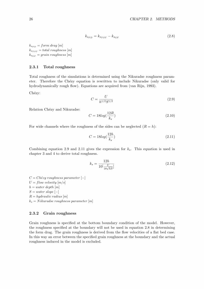
ksFD = ksTOT − ksGF (2.8)
ksFD= form drag [m]
ksTOT= total roughness [m]
ksGF= grain roughness [m]
2.3.1 Total roughness
Total roughness of the simulations is determined using the Nikuradse roughness param-eter. Therefore the Chezy equation is rewritten to include Nikuradse (only valid forhydrodynamically rough flow). Equations are acquired from (van Rijn, 1993).
Chezy:
C =U
h1/2S1/2(2.9)
Relation Chezy and Nikuradse:
C = 18log(12R
ks) (2.10)
For wide channels where the roughness of the sides can be neglected (R = h):
C = 18log(12h
ks) (2.11)
Combining equation 2.9 and 2.11 gives the expression for ks. This equation is used inchapter 3 and 4 to derive total roughness.
ks =12h
10[ U18√hS
](2.12)
C = Chezy roughness parameter [−]
U = flow velocity [m/s]
h = water depth [m]
S = water slope [−]
R = hydraulic radius [m]
ks = Nikuradse roughness parameter [m]
2.3.2 Grain roughness
Grain roughness is specified at the bottom boundary condition of the model. However,the roughness specified at the boundary will not be used in equation 2.8 in determiningthe form drag. The grain roughness is derived from the flow velocities of a flat bed case.In this way an error between the specified grain roughness at the boundary and the actualroughness induced in the model is excluded.

Chapter 3
Model calibration and validation
In order to validate the free surface OpenFOAM model two validation cases are modelled.The first validation consists of a flow over a straight bed in order to check the fundamentalsof the free surface model. This case is called the flat bed case and experiences only grainroughness. Therefore the flow properties can easily be compared to known theoretical flowphysics. After the fundamentals of the free surface model are proven to work, a secondvalidation is carried out comparing the free surface model outcome to measurements offlow over dunes.
3.1 Flat bed validation
The flat bed validation compares modelled velocities to theoretical velocities for flow overa straight bed (figure 2.1). Due the straight bed, total roughness consists of only grainroughness. The grain roughness is specified in the input parameters of the model, alongwith water depth and bed slope. The runtime of the free surface model is set long enoughfor the solution to converge and reach a equilibrium state. Convergence of the solutionof the free surface model is ensured by monitoring the Courant number and residuals(appendix C). From this equilibrium state, the output flow velocities are used to calculatethe grain roughness in the model (equation 2.12). The models works correctly if thederived grain roughness is similar to the grain roughness as specified input parameter.Therefore the difference between the input grain roughness and derived grain roughnessis one of the indicators of the performance of the model.
An other indicator of the performance of the model, is to what extent the modelled velocityprofile fits the logarithmic velocity profile. The logarithmic velocity profile is defined byequation 3.1 and is controlled by the water depth, water slope and grain roughness (vanRijn, 1993).
27

28 CHAPTER 3. MODEL CALIBRATION AND VALIDATION
u =u∗κln(
h
z0) (3.1)
u = velocity [m/s]
u∗ = shear velocity [m/s]
h = water depth [m]
κ = V on Karman constant [−] = 0.4
z0 = roughness height [m] = 30ks
The flat bed validation is conducted using lab scale dimensions, since the dune validationis carried out on lab scale as well. The following flow parameters are used for the flat bedvalidation:
Flat bed validation flow parameters :
Waterslope = 5 ∗ 10−4 [−]
Water depth = 0.5 [m]
ks = 0.01 [m]
z0 = csE ∗ ks
3.1.1 Model results
The mesh created for flat bed validation consists of 32 cells in the water column, whichgradually refine towards the bottom. This is a lot more than required (according to theguidelines in section 2.1.6). However, the air is modelled as well using the same cell sizeas the water surface. Therefore cells towards the water surface may not get too coarse.The area above the water, the atmospheric region, is modelled by 10 equally sized cells.The mesh and the dimensions of the flat bed model are shown in figure 3.1 and is labelledby ’Flat bed 1a’.
The logarithmic (equation 3.1) and modelled velocity profile are shown in figure 3.2. Closeto the bottom, the modelled velocity profiles fits the logarithmic profile very well. How-ever, moving upwards in the water column the modelled profile clearly deviates from thelogarithmic profile. In that section the modelled profile ends up vertical, while the loga-rithmic profile still follows its logarithmic definition (equation 3.1). This is no error in themodel, since measurements have shown the velocity profile in a water column consists ofboth a logarithmic and a parabolic part (Kundu and Ghoshal, 2012). The lower part ofthe velocity profile acts logarithmic while towards the surface acts increasingly parabolic.
In table 3.1 the average velocity of both profiles are shown. The average velocity of thelogarithmic and modelled velocity profile are both numerically determined. From theseaverage velocities the roughness parameters Chezy, Nikuradse and the roughness heightz0 are extracted.
Table 3.1 shows that the average velocity of the logarithmic and modelled profile areslightly different. The derived roughness parameters based on the flow velocities thereforeshow slight differences. The model performs well with an error of 0.7%. Further, thelogarithmic velocity profile does not exactly match the recalculated roughness height.This may be the cause of the chosen κ parameter or small deviations for the assumptionsmade for equation 2.12.

3.1. FLAT BED VALIDATION 29
Figure 3.1: Mesh and dimensions of the flat bed validation (Flat bed 1a)
Figure 3.2: Theoretical versus modelled velocity profile (flat bed case 1a)

30 CHAPTER 3. MODEL CALIBRATION AND VALIDATION
Table 3.1: Specified roughness (input) compared to the roughness based on the averagevelocity of the logarithmic and modelled velocity profile (flat bed case 1a)
3.1.2 Sensitivity analysis
In numerical modelling the model output is mesh depended. Therefore the magnitudeof this dependence should be very small compared to the magnitude of the solution. Inorder to check the magnitude of mesh dependence of the flat bed validation (flat bed 1a)several mesh adjustments are made (flat bed 2 and 3). However, in some cases (flat bed1b and 1c) not the mesh dependence, but the influence of the roughness constant (cs) isdetermined. In this way equation 2.5 is verified to be valid for OpenFOAM. Besides, twocases (flat bed 4a and 4b) are set up to check some refinement capabilities which are usedfor the experimental dune configurations in chapter 4. In order to give a full overview ofall cases, ’flat bed 1a’ is also added to the list below. Besides, in appendix D the mesh forall flat bed cases is visualised.
• Flat bed 1a: cs value 0.327This case is used for the flat bed validation (figure 3.1).
• Flat bed 1b: cs value 0.5This is a copy of ’flat bed 1a’, however the roughness constant cs is changed to 0.5.
• Flat bed 1c: cs value 1.0This is a copy of ’flat bed 1a’, however the roughness constant cs is changed to 1.0.
• Flat bed 2: Surface refinementFor this case the mesh around the surface is refined. Since the model solves both the water
and air particles, it is interesting to check weather the resolution of the transition from water
to air influences the modelled velocities.
• Flat bed 3: Total refinementFor this case the model consists of all equally small cells, to check if the resolution of the
mesh in the other cases is fine enough.
• Flat bed 4a: Bottom refinement using SnappyHexMeshSnappyHexMesh is a tool which comes with OpenFOAM to adjust meshes. In this case,
SnappyHexMesh is used for local refinement at the bottom of the model.
• Flat bed 4b: Partly bottom refinement using SnappyHexMesh In perspective to the
dune cases, it is expected the mesh is refined at some specific locations (for example the flow
separation zone) and not covering the whole length of the model. Therefore this case tests
if the model performs well by partly refining the mesh near the bottom.

3.2. DUNE CALIBRATION AND VALIDATION 31
The sensitivity of the velocity profiles and derived roughness parameters (equation 2.12)is visualised in figure 3.3 and table 3.2. According to the velocity profiles, the sensitivityof the velocities on the different mesh settings is low. All cases are in high agreement atthe bottom, and only have minor velocity differences occur towards the surface. However,these minor differences do have their influence on the average velocity based roughness(table 3.2). From this table, it can be concluded changing the roughness constant (andremaining the value of z0) does not affect the solution. Further, flat bed 2 and 4b performthe worst, however the differences of respectively 2.8% and -4.2% are still very acceptable.The high resolution mesh of flat bed 3 shows not to perform exceptionally better than theother cases. It performs even slightly worse than flat bed 1, which is expected to be theresult of the relatively high aspect ratio of the cells. In contrast to all flat bed cases, flatbed 1a still performs very reasonable.
Figure 3.3: Velocity profiles of all flat bed cases
Table 3.2: Sensitivity in grain roughness output parameters
3.2 Dune calibration and validation
McLean et al. (1999b) conducted a series of laboratory experiments of which one is used forthe dune validation. They used concrete to create asymmetric dune shapes. They did not

32 CHAPTER 3. MODEL CALIBRATION AND VALIDATION
determine the grain roughness of the material used for these dune shapes. Since the grainroughness is an important input parameter for the free surface model, another experimentof McLean et al. (1999b) is used to calibrate the grain roughness. The roughness obtainedfrom the dune calibration is then used as input for the dune validation.
The second (from now ML2) and sixth (from now ML6) laboratory setup of McLean et al.(1999a) are used for respectively calibration and validation of the free surface model. TheML2 dune case is calibrated on total roughness by adjusting the grain roughness. Thetotal roughness for the flume experiments is derived (making use of equation 2.12) frommeasured flow velocity, water depth and water slope. The ML6 dune case is validated byvelocity profiles, flow separation zone and again the total roughness.
Lefebvre et al. (2013) have modelled all the experiments of McLean et al. (1999b) inDelft3D, therefore the results of OpenFOAM are also compared to the output of Delft3Din appendix E.
• Dune case ML2Dune dimensions : height 0.04 [m] length 0.807 [m]
Waterslope = 9.5 ∗ 10−4 [−]
Water depth = 0.158 [m]
Grain roughness1 z0 = 0.00018 [m]
• Dune case ML6Dune dimensions : height 0.04 [m] length 0.408 [m]
Waterslope = 10.2 ∗ 10−4 [−]
Water depth = 0.3 [m]
Grain roughness z0 = 0.00018 [m]
3.2.1 ML2 and ML6 mesh
The mesh created for the dune validation is based on the guidelines stated section 2.1.6.However, due the small scale of the experiments, it is hard to meet the y+ requirementsfor the whole model domain (values of at least 30). The first cell at the bottom wouldbecome to large in contrast to the bedform and the other cells. Therefore, the layer addedis a compromise of retaining enough accuracy and satisfying the y+ requirement for atleast a part of the dune. In this way the top of the stoss side meets the y+ requirements,while in the lee side and the lower part of the stoss side the y+ requirements are not met.This means accuracy is retained at the flow separation zone at the expense of meeting they+ requirement. This can be justified by the idea that the magnitude of the form drag isgreater than the grain roughness. Besides, the flow velocities in the flow separation zoneare relatively low and therefore grain roughness plays a less important roll. The meshcreated for both the dune validation cases are showed in figure 3.4 and figure 3.5.
1The grain roughness is found by calibration.

3.2. DUNE CALIBRATION AND VALIDATION 33
Figure 3.4: Mesh created for ML2 dune validation
Figure 3.5: Mesh created for ML6 dune validation
3.2.2 Calibration results ML2
The ML2 dune case is used to estimate the grain roughness of the experiments carriedout by McLean et al. (1999a). Therefore grain roughness is calibrated to achieve thesame modelled total Nikuradse roughness as derived from the ML2 experiment. Lefebvreet al. (2013) used the same case for calibration and found a grain roughness parameter ofz0 = 0.0002[m]. This value is used as a starting point, from which the most appropriatevalue (to use in OpenFOAM) is found to be z0 = 0.00018[m] (table 3.3).
Calibration of the roughness parameter as shown in table 3.3 is in fact based on theaverage velocity output of the model only. Therefore the velocity profiles (figure 3.6) and

34 CHAPTER 3. MODEL CALIBRATION AND VALIDATION
Table 3.3: ML2 - Calibration of z0 grain roughness parameter
the flow separation zone (figure 3.7) are also compared to the measurements of McLeanet al. (1999a). However, these comparisons are only used as a qualitative check.
In general, the modelled velocity profiles are in good agreement with the measured pro-files. However, at the stoss side of the dune modelled velocities are underestimated towardsthe bottom, while they are overestimated in the direction of the surface. On the otherhand, the velocity profiles in the flow separation zone show a good fit close to the bot-tom, but again overestimate the velocity towards the surface. Figure 3.7 verifies that theflow separation zone is accurately modelled. The flow separation zone derived from themeasurements is obtained from Paarlberg et al. (2007).
The differences between modelled and measured velocity profiles are likely to be resultof the side walls of the flume used in the experiments of McLean et al. (1999a). Theseside walls are usually made of glass and are very smooth, however they do influence theflow. The model is a 2DV approach of the experiment and therefore these side wallsare replaced by empty boundaries. These empty boundaries do not influence the flow.The grain roughness of the side walls and the bottom in the experiment is in the modelonly represented by the bottom. Therefore it is likely the modelled grain roughness isoverestimated to meet the measured average velocity. The velocities towards the bottomare therefore underestimated while the velocities towards the surface are overestimated.
Besides, it is likely there is a slight difference in the ML2 dune shape and the modelleddune shape. It is plausible the experimental ML2 shape had not the exact sinusoidal duneshape, since in figure 3.6 some of the measurements show up inside the bottom profile.

3.2. DUNE CALIBRATION AND VALIDATION 35
Figure 3.6: ML2 - Velocity profiles of measurements of McLean (black) and modelled byOpenFOAM (red). Velocities are scaled by a factor 10.

36 CHAPTER 3. MODEL CALIBRATION AND VALIDATION
Figure 3.7: ML2 - Flow separation zones of measurements of McLean (black dots) andOpenFOAM (red line)
3.2.3 Validation results ML6
The ML6 case is the actual validation of the model and uses the grain roughness parametergained from the ML2 calibration case. The flow velocity and total roughness parametersof the modelled ML6 case are shown in table 3.4. The average velocity of the modelslightly deviates from the measured flow velocity. The Chezy roughness equation (equa-tion 2.9) takes the average velocity linear into account and therefore the same differenceas the average velocity is found in the Chezy roughness parameter. However, the Niku-radse roughness parameter shows a high relative deviation. This does not indicate poormodel performance, since the Nikuradse parameter tends to be sensitive to small velocitydifferences due its logarithmic definition (equation 2.12).
Table 3.4: ML6 - Validation of flow velocities and total roughness
The velocity profiles (figure 3.8) and the flow separation zone (figure 3.9) show still a

3.2. DUNE CALIBRATION AND VALIDATION 37
good overall agreement with the measurements. Velocity profiles for the modelled andmeasured ML6 case show similar deviations like the profiles shown for the ML2 case. Atthe stoss side of the dune close to the bottom the modelled velocities are underestimated,while the modelled velocities towards the water surface exceed the measured velocities.Explanations for these deviations are given in section 3.2.2. Again, the velocity profilesin the flow separation zone fit very well. Figure 3.9 confirms the flow separation zone isdecently modelled.
3.2.4 Mesh sensitivity
Section 3.1.2 mentioned that in numerical modelling the output is mesh depended. For theflat bed case several mesh settings were tested to ensure the model output had a low meshdependency. For the dune validation however, due time limitations, the mesh sensitivityis not tested. Therefore it is explicitly stated the mesh sensitivity of the validation casesremains unknown for this research.
It is important to discuss to which extent this mesh sensitivity might reach. Therefore aview is given on the expectations of the mesh sensitivity for the dune validation cases.
The key property of the guidelines provided by Lefebvre et al. (2013) is to provide enoughcells on top of the dune and in the flow separation zone, for the rotational flow to occur.Highly decreasing the amount of cells makes the flow easier to ’attach’ the bottom profilein the flow separation zone. Therefore the flow separation decreases or is may be totallyabsent. Increasing the amount of cells should make the model output more accurate,however the difference in size of the first cell at the bottom compared to the other cellswould increase, which may influence the model output as well. For the flow separationzone it is expected that decreasing the mesh resolution would affect the model output themost compared to an increase of resolution.
The water column above the dunes is expected to show only slight dependency to the mesh.The flow in this region is largely horizontal oriented without high turbulence aspects andthe increase of the dune over the stoss side is relatively gentle. Therefore this part of themodel has some similarities with the flat bed case, which shows a low mesh dependenceof the model output.
Analysing the mesh sensitivity of the dune validation cases is in particular useful for theflow separation zone. However, the provided guidelines and the results of both validationcases give confidence in a low, but unknown, mesh dependency.

38 CHAPTER 3. MODEL CALIBRATION AND VALIDATION
Figure 3.8: ML6 - Velocity profiles of measurements of McLean (black) and modelled byOpenFOAM (red). Velocities are scaled by a factor 20.

3.2. DUNE CALIBRATION AND VALIDATION 39
Figure 3.9: ML6 - Flow separation zones of measurements of McLean (black dots) andOpenFOAM (red line)

40 CHAPTER 3. MODEL CALIBRATION AND VALIDATION

Chapter 4
Model experiments
The created (chapter 2) and validated (chapter 3) free surface OpenFOAM model is used inthis chapter to conduct several experiments. The experiments consist of modelling the flowover different dune configurations which are defined in the first section. In the followingsections the model settings, model results and resulting form drag of the experimentaldune configurations are discussed.
4.1 Dune configurations
In this section three experimental dune configurations are defined. Dune dimensions andshapes are based on the measurements and shapes discussed in the articles and reports ofJulien et al. (2002), Wilbers and Ten Brinke (2003), McLean et al. (1999b), Ogink (1989)and Warmink et al. (2012) (figure 4.1). Therefore, the primary dunes as well as secondarydunes consist of typically sinusoidal stoss sides and straight 30◦ lee sides. The height andlength of dunes is scaled by factor 1
10 to ensure the dimensions are of the same magnitudeas the validation cases (chapter 3).
Figure 4.1: Measured dune dimensions (Julien et al. (2002); Wilbers and Ten Brinke(2003)) and experimental or hypothetical dune shape properties (McLean et al. (1999a);Ogink (1989); Warmink et al. (2012))
41

42 CHAPTER 4. MODEL EXPERIMENTS
The first dune configuration, the ’secondary dune’, is a relatively small and short dune.This secondary dune represents bed forms at the first stage of the proposed model of bedform evolution (figure 1.2). The second dune configuration is called the ’primary dune’and consist of a long and high single dune profile. This primary dune is comparableto the maximum dune heights occurring during floods (third stage of proposed bedformevolution model). The third dune configuration consists of a combination of primary andsecondary dunes which may be linked to the last two stages of the proposed bedformevolution model. Aside from the dune configurations, a straight bed case is modelled toderive grain roughness of the dune cases.
For all experimental dune configurations and the flat bed case the same flow conditionsapply. Therefore grain roughness, average water depth, water slope and bed form volumeare remained unchanged for all cases.
Summary of the model experiments:
• Case 0 - Flat bedStraight bed. Water level: 0.45 [m] Average water depth: 0.45 [m]
• Dune case 1 - Secondary duneHeight: 0.03 [m] Length: 0.7 [m] Water level: 0.465 [m] Average water depth: 0.45 [m]
• Dune case 2 - Primary duneHeight: 0.1 [m] Length: 4 [m] Water level: 0.5 [m] Average water depth: 0.45 [m]
• Dune case 3 - Primary dune containing secondary dunesDune dimensions of primary and secondary dune. Water level: 0.5 [m] Average water depth:
0.45 [m]
Figure 4.2: Dune case 1: Secondary dune
4.2. MODEL SETTINGS 43
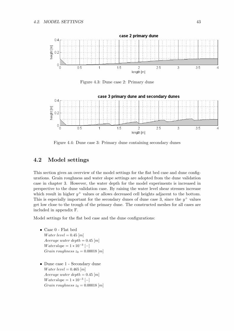
Figure 4.3: Dune case 2: Primary dune
Figure 4.4: Dune case 3: Primary dune containing secondary dunes
4.2 Model settings
This section gives an overview of the model settings for the flat bed case and dune config-urations. Grain roughness and water slope settings are adopted from the dune validationcase in chapter 3. However, the water depth for the model experiments is increased inperspective to the dune validation case. By raising the water level shear stresses increasewhich result in higher y+ values or allows decreased cell heights adjacent to the bottom.This is especially important for the secondary dunes of dune case 3, since the y+ valuesget low close to the trough of the primary dune. The constructed meshes for all cases areincluded in appendix F.
Model settings for the flat bed case and the dune configurations:
• Case 0 - Flat bedWater level = 0.45 [m]
Average water depth = 0.45 [m]
Waterslope = 1 ∗ 10−3 [−]
Grain roughness z0 = 0.00018 [m]
• Dune case 1 - Secondary duneWater level = 0.465 [m]
Average water depth = 0.45 [m]
Waterslope = 1 ∗ 10−3 [−]
Grain roughness z0 = 0.00018 [m]

44 CHAPTER 4. MODEL EXPERIMENTS
• Dune case 2 - Primary duneWater level = 0.5 [m]
Average water depth = 0.45 [m]
Waterslope = 1 ∗ 10−3 [−]
Grain roughness z0 = 0.00018 [m]
• Dune case 3 - Primary dune containing secondary dunesWater level = 0.5 [m]
Average water depth = 0.45 [m]
Waterslope = 1 ∗ 10−3 [−]
Grain roughness z0 = 0.00018 [m]
4.3 Model output
Output of modelled flow for the flat bed case and the experimental dune configurations iscovered in this section. For each of the simulations horizontal flow velocities and stream-lines are depicted. Streamlines visualise the path of the water particles from which theflow separation zones are easily observed. The air region of the model domain is recognisedby the lack of these streamlines.
Turbulent fluctuations induced by the flat bed case and dune cases are visualised bythe Turbulent Kinetic Energy (TKE) plots. The intensity of the TKE reveals the highturbulent regions of the flow which contribute to form drag.

4.3. MODEL OUTPUT 45
4.3.1 Case 0 - Flat bed
Simulation of the flat bed case results in an uniform horizontal velocity field (figure 4.5)and TKE plot 4.6. The streamlines show that flow is horizontally orientated. From theTKE plot is seen TKE increases from the surface towards the bottom. This is the effect ofgrain roughness acting on the flow. However, in comparison to the dune cases the intensityof the TKE is relatively low.
Figure 4.5: Case 0 - Flat bed: Horizontal velocities and streamlines
Figure 4.6: Case 0 - Flat bed: Turbulent kinetic energy
46 CHAPTER 4. MODEL EXPERIMENTS
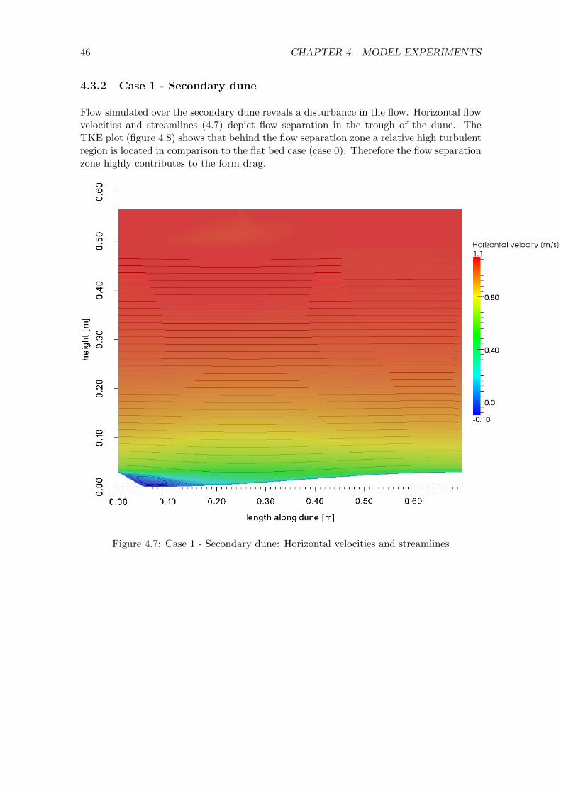
4.3.2 Case 1 - Secondary dune
Flow simulated over the secondary dune reveals a disturbance in the flow. Horizontal flowvelocities and streamlines (4.7) depict flow separation in the trough of the dune. TheTKE plot (figure 4.8) shows that behind the flow separation zone a relative high turbulentregion is located in comparison to the flat bed case (case 0). Therefore the flow separationzone highly contributes to the form drag.
Figure 4.7: Case 1 - Secondary dune: Horizontal velocities and streamlines

4.3. MODEL OUTPUT 47
Figure 4.8: Case 1 - Secondary dune: Turbulent kinetic energy
4.3.3 Case 2 - Primary dune
Flow over the primary dune shows the same aspects of the flow like the secondary dune case(case 1). In the trough of the dune flow separation occurs (figure 4.9) and the TKE plot(figure 4.10) shows that a high intensity of turbulence located behind the flow separationzone. However, the dimensions of the primary dune are much larger than the secondarydune case. The primary dune is about three times higher and six times longer. The TKEplot shows that the high turbulent region is about eight times longer for the primary dunecase in perspective to the secondary dune case.

48 CHAPTER 4. MODEL EXPERIMENTS
Figure 4.9: Case 2 - Primary dune: Horizontal velocities and streamlines
Figure 4.10: Case 2 - Primary dune: Turbulent kinetic energy
4.3.4 Case 3 - Primary dune and secondary dunes
The simulation of flow over the combination of primary and secondary dunes shows that inall troughs of the dune shapes flow separation occurs (figure 4.11). However, the intensityof the turbulent regions varies for the different secondary dunes (figure 4.12). Secondarydunes placed low on the stoss side of the primary dune induce a lower TKE than secondarydunes located more towards the crest of the primary dune. The secondary dune closestto the primary dune crest shows to induce similar or slightly higher turbulent intensitiescompared to the secondary dune case (case 1).
The turbulent region induced by the flow separation zone of the primary dune part has alower intensity than to the primary dune case (case 2). However, the size of the wake ofthe turbulent region is similar.

4.4. FORM DRAG OF THE EXPERIMENTAL DUNE CONFIGURATIONS 49
Figure 4.11: Case 3 - Primary dune containing secondary dunes: Horizontal velocities andstreamlines
Figure 4.12: Case 3 - Primary dune containing secondary dunes: Turbulent kinetic energy
4.4 Form drag of the experimental dune configurations
The form drag of the experimental dune configuration is derived in this section. Formdrag is defined by the difference in total roughness and grain roughness (section 2.3).
The flow velocity of the experimental cases is used to derive total roughness (equation2.12). Grain roughness for the dune configurations is obtained from the flat bed case (case0). The grain roughness for dune configurations is not corrected for bed form influences(e.g. the flow separation zone or increased surface length) since the form drag is generallydominant over the grain roughness (Knighton (1998) and Julien et al. (2002)). The dom-inance of form drag over grain roughness is also confirmed by results of the experimentaldune configurations (figure 4.13) and by the grain roughness sensitivity analysis (appendixG). Therefore it is assumed the grain roughness is not influenced by the presence of bedforms and is directly obtained from the flat bed case (case 0). The derived total roughnessof the experimental cases is shown in figure 4.13.
Form drag is derived by subtracting grain roughness from the total roughness. The formdrag of the dune configurations is shown in figure 4.1. The combination of primary andsecondary dunes (case 3) induces the largest amount of form drag, followed by the formdrag induced by the primary dune (case 2). The secondary dune case (case 1) has thelowest form drag. Figure 4.1 also shows that the form drag of dune case 3 is larger than

50 CHAPTER 4. MODEL EXPERIMENTS
Figure 4.13: Total Nikuradse roughness of the three dune cases and the flat bed case
the summation of form drag induced by the separated dune shapes (case 1 and case 2).
Table 4.1: Nikuradse form drag of the experimental dune configurations
Chapter 5
Discussion
In the introduction (chapter 1) the principles of grain roughness and form drag werediscussed. The highly changing bed forms of the proposed bed form evolution processof Warmink et al. (2012) indicated that form drag during flood waves is likely to change.Three typical dune configuration were defined (chapter 4) which are related to the bed formstages defined in the proposed bed form evolution process. By flow modelling over thesedune configuration the form drag is determined based on the occurring flow velocities.
This chapter couples the experimental results to the proposed bed form evolution process.Besides, the most important assumptions of the model and proposed improvements of themodel set up are discussed.
5.1 Roughness variability during flood waves
The proposed bed form evolution process visualised in figure 1.2 consists of six separatedbed form stages. The results of the three modelled dune configurations are used to describethe total roughness variation through these stages.
5.1.1 Form drag of bed form evolution stage 1, 2 and 3
The first two stages of the proposed dune evolution process show how smaller dunesincrease in length and height, while the discharge increases. The third stage shows thatthis process continuous until the peak discharge has just passed.
Bed forms of the first and third stage are comparable to respectively the secondary dune(case 1) and primary dune (case 2) configuration (chapter 4). Comparing the flow sepa-ration zones of the secondary and primary dune (figure 4.7 and 4.9), the flow separationzone of the primary dune is about 4 times the size of the flow separation zone of thesecondary dune. Besides, the flow separation zone of the secondary dune is steeper (about4 to 5 times the secondary dune height) than the flow separation zone of the primary dune(about 6 times the primary dune height). Lefebvre et al. (2013) also observed that smallerbed forms generate shorter and steeper flow separation zones.
Based on the flow separation zones the form drag is expected to be larger for the primarydune (case 2) than the secondary dune (case 1) configuration. This is confirmed by figure
51

52 CHAPTER 5. DISCUSSION
4.1 which shows that the primary dune configuration induces about 1.8 times the form dragof the secondary dune configuration. This factor is slightly smaller for the total roughness:about 1.6 (figure 4.13). Julien et al. (2002) measured an increase of total roughness withincreasing discharge, which is also attributed to bed form height. Therefore it is concludedthe form drag and total roughness increases for the first three stages of the bed formevolution process due to the increase of form drag.
5.1.2 Form drag of bed form evolution stage 4, 5 and 6
The last three stages of the proposed bed form evolution process represent the behaviourof bed forms during the falling stage of the flood. The large primary dunes from the thirdstage still increase in length but decrease in height during these last stages. In the fifthand the sixth stage the angle of repose of the primary dune lowers and secondary dunesmigrate on top of the primary dunes.
The primary dune containing secondary dunes (case 3) configuration (chapter 4) is compa-rable to the fifth and sixth stage of the proposed bed form evolution process. The primaryshape of dune case 3 is similar to dune case 2, while the secondary shapes were obtainedfrom dune case 1. Therefore, the primary dune shape of this dune configuration does notshow the lowering in angle and increase in length proposed by the bed form evolutionprocess. However, the dune configuration of case 3 does reveal the influence of secondarydunes submerged on primary dunes.
Figure 4.11 shows that flow separation is present for all troughs of the primary and sec-ondary dune shapes. However, the streamlines are not accurate enough to distinguishdifferences in flow separation zones in comparison to case 1 and case 2. From the TKE de-picted in figure 4.12 differences are more clearly seen to the secondary dune case 1 (figure4.8) and primary dune case 2 (figure 4.10). The intensity of TKE appears to be higher inthe troughs of separately modelled dunes in case 1 and case 2 compared to the intensity ofTKE of the troughs in case 3. However, the submerged secondary dune closest to the topof the primary shape shows about the same TKE as the secondary dune shape of case 1.This can be explained by the higher velocities over this secondary dune compared to thelower placed secondary dunes (figure 4.11). Fernandez et al. (2006) show that if secondarybed forms are even closer to the top of the primary bed form, interaction of the flow sep-aration zones may occur which lead to high levels of turbulence intensity. Therefore thelocation of secondary dunes on the primary shape shows to be important for the intensityof the TKE.
Figure 4.1 shows that case 3 induced the highest form drag of all experimental duneconfigurations. The form drag of case 3 is even higher (approximately 1.1 times) thansummation of the form drag of case 1 and case 2. In comparison to the primary dune(case 2) form drag is multiplied by a factor of about 1.8 if the same dune consists ofmerged secondary dunes. For total roughness this factor is about 1.6 (based on figure4.13).
Total roughness of the bed forms occurring in the fifth and sixth stage of the proposedbed form evolution process may therefore still increase. However, following the bed formevolution process the primary shape in these stages lowers and flattens. This effect innot included in case 3 but may decrease the total roughness substantially (Best, 2002).Therefore simulations or measurements of additional dune configurations are required tounderstand the variations of form drag in the fifth and sixth stage.

5.2. MODEL ASSUMPTIONS 53
5.2 Model assumptions
In order to put the conclusions and statements of this chapter in the right perspective,important assumptions and decisions of the model and the dune configurations are sum-marized in this section. Discussed is how these assumptions and decisions may influencethe form roughness of the 6 stages of the bed form evolution process.
5.2.1 Laboratory scale versus field scale
The dune configurations, grain roughness, slope and water depth were all scaled to labora-tory dimensions. The model results of the experimental dune configurations are reliable,since similar model settings and dimensions were used for the model validation. On theother hand, the question arises if the flow predicted by a laboratory scale model is repre-sentative for field scale conditions. In general for laboratory conditions the grain roughnessand water depth are relatively small while the slope is relatively steep. For the field scaleconditions it is generally the other way around.
The work of Lefebvre et al. (2013) shows a scaling method for the laboratory and fieldscale dimensions. The scaling reveals for which field scale dimensions the results of thelaboratory scale apply. The scaling method consists of scaling all model properties (i.e.water depth, grain roughness, dune height, dune length) by a certain factor except for theslope. The slope is scaled in the counter direction. Using this method, the shear velocitiesat laboratory and field scale dimensions are similar.
In table 5.1 case 3 (chapter 4) is used as an example to show which field scale dimensionsapply to the results of the laboratory scale model. Therefore a scaling factor of 10 isused. This is the same factor as used in chapter 4 to scale the field dune dimensions tolaboratory scale dimensions. Table 5.1 shows that the dune dimensions and river slope areof the magnitude measured by Julien et al. (2002) and Wilbers and Ten Brinke (2003).However, the scaled grain roughness is relatively high and the water depth relatively smallcompared to measured river conditions.
The validity of the scaled grain and total roughness parameters is checked using one of thesimplest roughness estimators, the roughness model of van Rijn (1993). The mathematicaldefinition of the roughness parameter is given by equation 5.1. Using the field scaledimensions of the dune configurations (scaling factor of 10 is used) the roughness estimatoroverestimates the total roughness for all cases (table 5.2). The increase in total roughnesswhen moving from case 1 to case 3 is however confirmed. The roughness model of vanRijn (1993) may be based on different dune shapes and flow conditions which could explainthe differences. However, based on the comparison in table 5.2 the validity of the modelresults for field scale conditions can not be confirmed. Although the order of magnitudeof the modelled total roughness shows to be reasonable.
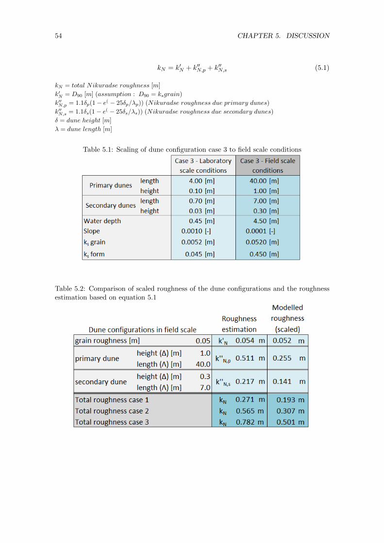
54 CHAPTER 5. DISCUSSION
kN = k′N + k′′N,p + k′′N,s (5.1)
kN = total Nikuradse roughness [m]
k′N = D90 [m] (assumption : D90 = ksgrain)
k′′N,p = 1.1δp(1− e( − 25δp/λp)) (Nikuradse roughness due primary dunes)
k′′N,s = 1.1δs(1− e( − 25δs/λs)) (Nikuradse roughness due secondary dunes)
δ = dune height [m]
λ = dune length [m]
Table 5.1: Scaling of dune configuration case 3 to field scale conditions
Table 5.2: Comparison of scaled roughness of the dune configurations and the roughnessestimation based on equation 5.1

5.2. MODEL ASSUMPTIONS 55
5.2.2 Static and idealized shaped bed forms
The shapes of all dune configuration are idealized bed forms, consisting of a sinusoidalstoss side and a 30◦ lee side angle. Besides the bed forms are static (no migration) andsediment transport is not part of the model. The static bed forms are in contradictionto the bed being in constant movement (chapter 1). However, due the relatively slowmorphological process it is appropriate to neglect this effect.
The assumption of the typical asymmetrical dune shape consisting of an angle of reposeof 30◦ is believed to have a high impact on the form drag. Best (2002) discuss that inmany models of alluvial dunes these typical bed form shapes are assumed, while mostdunes in large sand bed rivers possess more symmetrical profiles, lower lee side angles,and flow separation that is either intermittent or absent. Many river bed forms wouldshow no permanent flow separation and the turbulent region behind the bed forms wouldbe much lower. Therefore it is arguable if the shapes of the experimental dune configura-tions (chapter 4) are representative for real bed forms in rivers. Nevertheless, these duneconfigurations show till which extent the roughness of form drag may reach.
5.2.3 2DV model versus 3D reality
In this research the width directional dimension of the flow is neglected and only the effectof two dimensional dune configurations is studied. However, in rivers the dunes vary inheight and length, as well as in the width directional dimension. Therefore the 2DV flowpattern along this dimension change as result of the change in bed form shape. Besides,2DH (horizontal plane) flow patterns become important as well.
The experiments of Maddux et al. (2003) show that averaged friction coefficients for flowover 3D (primary) bed forms was 50% higher than for the 2D shapes. However, despite thelarger friction of the 3D dunes, the turbulence generated by them was much weaker. Theincrease in friction coefficients is contributed to the higher spatial variability in near-bedvelocities and to the non-linear increase in skin friction induced by local high velocities.Grigoriadis et al. (2009) also shows different turbulent structures arising for 3D (primary)dune shapes. They used a large-eddy simulation to reveal spanwise roller coherent struc-tures to develop because of separation at the dune crest. However, at the reattachmentpoint they found horseshoe structures. Venditti (2007) shows both an increase and de-crease of the flow separation zone of 3D (primary) bed forms compared to flow over 2Ddune shapes. The magnitude of the flow separation of saddle shaped bed forms was lowerthan the flow separation over a lobe.
This research consists of a first exploration to secondary bed forms in 2DV. However,while the understanding of primary and secondary bed forms increases, the 3D modellingof primary and secondary dunes may be part of future research.

56 CHAPTER 5. DISCUSSION
5.3 Improvements of the model set up
Several improvements to the free surface OpenFOAM model are proposed in this section.
Regarding the reliability of the model it is important a comprehensive study to the meshsensitivity and the optimum mesh settings for free surface modelling in OpenFOAM isperformed. To further improve confidence in the model a validation based on measure-ments of a dune profile consisting of merged secondary dunes is useful. The performedvalidation in chapter 3 exists of only single dune profiles and it remains unknown if themore complex case 3 of the dune configuration is accurately modelled.
Another improvement refers to the way in which the model is used for determining theform drag. For computing the flow properties of the different dune configurations, eachtime the slope (horizontal bodyforce) is predefined in the model. Therefore the shearvelocity and bed shear stress do not change for the different cases. Only the velocitiesor discharge (since the water depth is remained) change as effect of the differences inform drag. However, for real river cases it is the discharge which always is assumed tobe remained. Therefore a general hydrodynamic model setup consists of a discharge inletand a controlled water level outlet. In order to maintain the benefits of the cyclic modelbut include a constant discharge, the slope (horizontal bodyforce) should be adjusted foreach case until a certain discharge is achieved. In this way the cyclic model can be usedto show the differences in total shear stress for each dune configuration.

Chapter 6
Conclusions and outlook
The first chapter defined the research objective: ’To provide a better understanding of theroughness variability during flood waves, by computing the form drag of typical primaryand secondary dune configurations in rivers’. The research questions were used to fulfil thisobjective. Section 6.1 shortly recaps each research question and summarizes the importantconclusions. An outlook for additional research is given in section 6.2.
6.1 Conclusions
Which model settings are used for creating a free surface model in OpenFOAM?In chapter 2 the model settings are explained. The interFoam solver is selected to create afree surface flow while the k-epsilon turbulence model is used for simulating the turbulenceaspects of the model. In order to able to work with a small model domain, cyclic boundaryconditions are implemented for which the interFoam solver is adapted to work properly.Two mesh restrictions show to be important for flow modelling in OpenFOAM. The y+
values should have a minimum value of 30 in order to properly model the grain roughness.For the same reason the ratio of the height of the cell centre to the grain roughness ksshould not exceed the value of 0.2.
How do the model results compare to a validation reference case?The validation of the model is subject of chapter 3. The flat bed validation shows to fitthe logarithmic velocity profile well and the grain roughness parameters obtained fromthe flow properties were in accordance to the input grain roughness of the model. Thedune validation is carried out by comparing the model results to a laboratory experiment.However, grain roughness was not defined for these experiments. Therefore one laboratoryexperiment is used for calibration of the grain roughness. The actual validation of a seconddune case was successful and shows a high agreement in measured and modelled velocityprofiles, flow separation zones and total roughness parameters. Therefore it is concludedthe model performs properly for modelling free surface flow.
What is the form drag of the investigated dune configurations?The simulation of the flow over the experimental dune configurations is part of chapter4. Long and high primary dunes (case 2) induce a higher form drag than the smallerand lower secondary dunes (case 1). However, the dune configuration consisting of bothprimary and secondary dunes (case 3) shows to induce the highest form drag. The form
57

58 CHAPTER 6. CONCLUSIONS AND OUTLOOK
drag of case 3 is even higher than the summation of the form drag of case 1 and cases 2.However, this does not directly follow from the turbulent kinetic energy plots. The TKEinduced behind the trough of the primary dune shape of case 3 is lower than the similarprimary dune shape of case 2. The secondary dune shapes of case 3 show divergent TKEintensities behind their troughs. The TKE intensities increase from the 1st secondarydune (close to the trough of the primary bed form) towards the last secondary dune closeto the crest of the primary bed form. The first three secondary bed forms induce a lowerTKE compared to case 1, while the last secondary dune induces approximately the sameamount of turbulence in perspective to case 1.
What are the variations in form drag during floods, following the proposed model of bedformevolution?Chapter 5 discusses the results of the experimental dune configurations in perspective tothe variances of the form drag during the floods using the proposed bed form evolutionprocess. Figure 1.2 refers to the bed evolution process consisting of six bed form stages.For the first three stages where the primary dunes are growing in both length and height isconcluded that the form drag increases. For the last three stages, where the primary dunekeeps increasing in length but decreases in height and secondary dunes start to occur, isconcluded that it is possible for these dune configurations to induce a higher form dragthan the high primary dunes of the 3th stage. The investigated dune configurations showform drag increases by a factor of 1.8 when secondary dunes occur on the primary dune.Therefore, secondary dunes merged on primary dunes add a significant amount of formdrag, but the effect of decay of primary dunes in these stages is not determined. It dependson actual primary and secondary bed form shape and dimensions if form drag increasesor decreases during the falling stage of a flood wave.
6.2 Outlook
The conclusions of this research are based on an exploratory investigation to form drag ofprimary and secondary dune configurations. Therefore many aspects of the dune shapeand dimensions are not varied even though these definitely have their influence on the formdrag. This section discusses the areas in which research should be continued to verify theapplicability of the stated conclusions and gain a better understanding of the form dragduring floods.
This research shows that the influence of primary and secondary bed forms are importantfor the development of turbulences inducing form drag to the flow. Nevertheless there isyet much to discover about primary bed forms and superimposed secondary bed forms.Changes in shape and dimensions of both the primary and superimposed secondary bedforms should be researched in order to improve the understanding of form drag duringfloods. Besides the influence of variations to the location of the superimposed secondarybed forms may be studied, which show to be important for the amount of turbulenceinduced by the superimposed secondary bed form. Actual knowledge of these influencesis for now insufficient to fully understand form drag variations during the bed evolutionprocess. In general, more dune configurations should be researched in order to these formdrag variations.
In future research 3D modelling may also be considered. Measurements (i.e. Venditti(2007) and Maddux et al. (2003)) and 3D modelling (Grigoriadis et al., 2009) already showfor some primary bed form cases the total roughness by the 2D shapes is underestimated.

6.2. OUTLOOK 59
However, 3D modelling is complex and time consuming due high computer processorrequirements.
This research shows the form drag of primary and superimposed secondary bed forms isof high importance to total roughness of rivers. Proposed additional research may leadto better understanding and prediction of total roughness of specific dune configurations.This information could then be used to implement variable roughness parameters in thenumerical models predicting the design water levels (chapter 1).

60 CHAPTER 6. CONCLUSIONS AND OUTLOOK

Bibliography
Best, J. (2002). An experimental study of turbulent flow over a low-angle dune. Journalof Geophysical Research, 107(C9):3135.
Best, J. (2005). The fluid dynamics of river dunes: A review and some future researchdirections. Journal of Geophysical Research, 110(F4):F04S02.
Booij, R. (1992). TURBULENTIE in de waterloopkunde. Technische Universiteit Delft.
Engelund, F. (1967). A monograph on sediment transport in alluvial streams by FrankEngelund and Eggert Hansen. Teknisk Forlag.
Fernandez, R., Best, J., and Lopez, F. (2006). Mean flow, turbulence structure, andbed form superimposition across the ripple-dune transition. Water Resources Research,42(5).
Grigoriadis, D. G. E., Balaras, E., and Dimas, a. a. (2009). Large-eddy simulations ofunidirectional water flow over dunes. Journal of Geophysical Research, 114(F2):F02022.
Julien, P. Y., M.ASCE, Klaassen, G. J., Brinke, W. B. M. T., and Wilbers, A. W. E.(2002). Case Study : Bed Resistance of Rhine River during 1998 Flood. Journal ofHydraulic Engineering, 128(12):1042–1050.
Knighton, D. (1998). Fluvial Forms and Processes: A New Perspective. A Hodder ArnoldPublication. Arnold.
Kundu, S. and Ghoshal, K. (2012). Velocity Distribution in Open Channels : Combinationof Log-law and Parabolic-law. World Academy of Science, Engineering and Technology,68:1735–1742.
Lefebvre, A., Paarlberg, A. J., and Winter, C. (2013). Flow separation and shear stressover angle of repose bedforms: a numerical investigation. Water Resources Research,49(10).
Liu, X., Garcıa, M. H., and Asce, M. (2008). Three-Dimensional Numerical Model withFree Water Surface and Mesh Deformation for Local Sediment Scour. Journal of Wa-terway, Port, Coastal, and Ocean Engineering, (August):203–217.
Maddux, T. B., Nelson, J. M., and McLean, S. R. (2003). Turbulent flow over three-dimensional dunes: 1. Free surface and flow response. Journal of Geophysical Research:Earth Surface, 108(F1).
Martinez, B. (2011). Wind resource in complex terrain with OpenFOAM. PhD thesis,Technical University of Denmark.
61

62 BIBLIOGRAPHY
McLean, S., Wolfe, S., and Nelson, J. (1999a). Predicting Boundary Shear Stress andSediment Transport over Bed Forms. Journal of Hydraulic Engineering, 125(7):725–736.
McLean, S. R., Wolfe, S. R., and Nelson, J. M. (1999b). Spatially averaged flow over a wavyboundary revisited. Journal of Geophysical Research: Oceans, 104(C7):15743–15753.
Moradnia, P. (2010). CFD of Air Flow in Hydro Power Generators. Technical report,Chalmers University of Technology, Goteborg, Sweden.
Ogink, H. J. M. (1989). Hydraulic Roughness of Single and Compound Bed Forms. DelftHydraulics.
OpenFOAM Foundation (2012). OpenFOAM, The Open Source CFD Toolbox - UserGuide version 2.1.1. Technical report.
OpenFOAM Foundation (2013). Standard Solvers.
Paarlberg, A. J., Dohmen-Janssen, C. M., Hulscher, S. J. M. H., and Termes, P. (2007). Aparameterization of flow separation over subaqueous dunes. Water Resources Research,43(12):W12417.
Pattanapol, W., Wakes, S. J., Hilton, M. J., and Dickinson, K. J. M. (2007). Modeling ofSurface Roughness for Flow Over a Complex Vegetated Surface. Proceedings of worldacademy of science, engineering and technology, 26(December).
Salim, S. M. and Cheah, S. C. (2009). Wall y + Strategy for Dealing with Wall-boundedTurbulent Flows. Proceedings of the International MultiConference of Engineers andComputer Scientists, II.
Van Rijn, L. C. (1984). Sediment transport, part {III:} bed forms and alluvial roughness.Journal of Hydraulic Engineering, 110(12):1733–1754.
van Rijn, L. C. (1993). Principles of sediment transport in rivers, estuaries and coastalseas. Number dl. 1 in Principles of Sediment Transport in Rivers, Estuaries, and CoastalSeas. Aqua Publications.
Venditti, J. G. (2007). Turbulent flow and drag over fixed two- and three-dimensionaldunes. Journal of Geophysical Research, 112(F4):F04008.
Warmink, J., Dohmen-Janssen, C., and Schielen, R. (2012). Bed form evolution undervarying discharges, flume versus field. In River Flow 2012, pages 183–190. CRC Press.
Wilbers, A. and Ten Brinke, W. (2003). The response of subaqueous dunes to floods insand and gravel bed reaches of the Dutch Rhine. Sedimentology, 50(6):1013–1034.

Appendix A
Technical details boundaryconditions
The technical details of the boundary conditions used in the OpenFOAM model are sum-marized in table A.1. Most of the settings (including the numerical scheme) are obtainedfrom the ’dam break’ tutorial of OpenFOAM Foundation (2012).
Table A.1: Technical details of the used boundary conditions in the OpenFOAM model
63

Appendix B
Adapted interFoam solver
The full code of the adapted UEqn.h file of the interFoam solver is covered in figure B.1.
Figure B.1: Adapated UEqn.h file of the interFoam solver
64

Appendix C
Convergence of the solutionsgenerated by the free surfaceOpenFOAM model
To ensure the output of the free surface model is converged the Courant numbers and theresiduals of the solutions are monitored. The Courant numbers and residuals showed infigure C.1 and C are obtained from the same timestep as the output shown in chapter 3and 4.
Figure C.1: Residuals and Courant numbers of the flat bed validation
Table C.1: Residuals and Courant numbers of the dune validation and model experiments
65

Appendix D
Sensitivity analysis flat bed case
Several mesh adjustments to the flat bed case have been made in order to determine themesh dependence of the model output. The meshes corresponding to the cases mentionedin chapter 3 are visualised in this appendix. The water depth in each of these models isset to 0.5 meter.
Figure D.1: Mesh used for flatbed 1a, 1b and 1c (varying roughness constant cs)
66

67
Figure D.2: Mesh used for flatbed 2 (surface refinement)
Figure D.3: Mesh used for flatbed 3 (total refinement)

68 APPENDIX D. SENSITIVITY ANALYSIS FLAT BED CASE
Figure D.4: Mesh used for flatbed 4a (bottom refinement using SnappyHexMesh)
Figure D.5: Mesh used for flatbed 4b (partly bottom refinement using SnappyHexMesh)

Appendix E
Dune validation cases includingDelft3D results
The Delft3D results achieved by Lefebvre et al. (2013) are added to the dune validationcases ML2 and ML6. Velocity profiles of both cases are compared in figure E.1 and E.3.The comparison of flow separation zones is shown in figure E.2 and E.4. The modelledDelft3D velocities near the bottom sometimes appear below the bed. This is likely theresult of the Cartesian grid used by Lefebvre et al. (2013). Therefore diagonal bed shapesare modelled as a staircase.
69

70 APPENDIX E. DUNE VALIDATION CASES INCLUDING DELFT3D RESULTS
Figure E.1: ML2 - Velocity profiles of measurements of McLean (black), modelled byDelft3D (blue) and modelled by OpenFOAM (red). Velocities are scaled by a factor 1
10 .

71
Figure E.2: ML2 - Flow separation zones of measurements of McLean (black dots), Delft3D(blue dots) and OpenFOAM (red line)

72 APPENDIX E. DUNE VALIDATION CASES INCLUDING DELFT3D RESULTS
Figure E.3: ML6 - Velocity profiles of measurements of McLean (black), modelled byDelft3D (blue) and modelled by OpenFOAM (red). Velocities are scaled by a factor 1
10 .

73
Figure E.4: ML6 - Flow separation zones of measurements of McLean (black dots), Delft3D(blue dots) and OpenFOAM (red line)

Appendix F
Constructed meshes for modelexperiments
The constructed meshes for all model experiments are depicted in figure F.2, F.3 and F.4.
Figure F.1: Flatbed: Mesh
74

75
Figure F.2: Case 1 - Secondary dune: Mesh
Figure F.3: Case 2 - Primary dune: Mesh

76 APPENDIX F. CONSTRUCTED MESHES FOR MODEL EXPERIMENTS
Figure F.4: Case 3 - Primary dune: Mesh

Appendix G
Sensitivity varying grainroughness
In order to gain insight in the sensitivity of the form drag to the grain roughness, the threedune cases are run again with a 20% higher and 20% lower grain roughness. Small changesin grain roughness are applied to be able to use the same mesh (see chapter 2.1.6 for meshrestrictions). Therefore no visual differences are noticed in figures of the horizontal flowvelocities or turbulent kinetic energy, however they do slightly change.
• Grain roughness variations:Decrease 20% : z0 = 0.000144 [m]
Default z0 = 0.00018 [m]
Increase 20% : z0 = 0.000216 [m]
Table G.1 summarizes the sensitivity results of the flatbed case and dune configurationsfor variations in grain roughness. The flat bed case shows to model the change in grainroughness well. The total Nikuradse roughness (for the flat bed case the grain roughness)derived from velocities of the model shows a decrease and increase of 19% for respectivelythe smoother and rougher grain roughness.
Results of the dune configurations show an interesting pattern. For all dune cases, anincrease in grain roughness also results in an increase in form roughness. Sensitivity of theform drag is however of a lower magnitude in perspective to the grain roughness variations.In general the form drag varies from around -8% to +12% in comparison to the ±19%variation of the grain roughness. Considering only case 3, containing the primary andsecondary dunes, this sensitivity is reduced to about ±5%.
77

78 APPENDIX G. SENSITIVITY VARYING GRAIN ROUGHNESS
Table G.1: Sensitivity of the average velocity, total roughness and form roughness incomparison to the variation of the grain roughness