[1]

DRAFT: METHODS FOR CONDUCTING A SUBAQUEOUS SOIL SURVEY

Introduction: The creation of subaqueous soil maps is an extension of the marine spatial planning

initiative that has been established for the entire marine environment. It is vital to include these shallow water areas in mapping as they are the most highly impacted and visible oceanic areas in everyday life. Estuaries and shallow coastal waters are some of the most productive habitats in the world, making up only 1-2% of the ocean area, yet supporting approximately 20% of oceanic primary production. Almost two-thirds of the worldwide population currently lives in coastal areas and recent demographic studies suggest that in the next 25 years 75% of the US population will be living near the coast. Despite being such highly valued and heavily used resources, it has become evident in recent years that the nation’s shoreline and shallow water areas are lacking in consistent and comprehensive baseline data. This data will be critical to managing risk and creating the adaptation strategies for the sea level rise and other impacts associated with climate change. In an effort to fill this data gap, the National Cooperative Soil Survey has begun to include shallow water soils in their mapping protocol. For over 100 years the National Cooperative Soil Survey has been responsible for documenting the nation’s soil resources using standard procedures and taxonomic naming systems across the country. These data provide valuable land use interpretations, land use histories, and a baseline of chemical and physical data that allow us to create new interpretations as need arises. These same protocols have recently been transferred to mapping subaqueous soils - soils found in intertidal areas to a depth of approximately 5 meters. Mapping these areas as soils allows for consistent data collection around the country by a network of trained scientists using already established data collection, naming, and mapping standards.

Soils on land develop in predictable patterns as a result of the climate, organisms that interact with the soil, topography of the land, parent material from which the soil developed, and the age of the soil or the amount of time the soil has been undergoing pedogenesis (Jenny, 1941). Soil types are repeated across the terrain and similar soils are consistently found in areas where soil forming factors act in a distinctive way (Hudson, 1990). Soils that form underwater have additional factors that control soil development including flow regime, water column attributes, catastrophic events, and bathymetry (Demas and Rabenhorst, 2001). Because subaqueous soils develop as a result of the environment in which they developed, these soils are a very good indication of many important estuarine properties including water quality attributes over time, past catastrophic events, changes in types or numbers of organisms over time, and changes in sea level over time. Current and accurate maps and baseline data allow for the development of interpretations based on this data. Currently subaqueous soil interpretations are in

[2]

development for carbon pools, and it has been shown that subaqueous soil organic carbon (SOC) pools are comparable to SOC pools in some terrestrial ecosystems and should be considered important global sinks that are currently unaccounted for (Pruett, 2010). Additional research on dredge disposal and the potential for acid sulfate soil creation has shown that certain subaqueous soils should not be deposited on land as beach replenishment or dredge disposal due to the potential to create highly acidic soil materials as a result of oxidation of sulfides (Salisbury, 2010). Identification of prime locations for shellfish aquaculture and replanting of seagrass are other needs of growing importance in coastal areas. Locations with high potential for successful oyster or seagrass restoration can be identified using subaqueous soils information, as well as locations that could provide prime aquaculture areas (Bradley and Stolt, 2006). Because subaqueous soils develop as a result of water column attributes and flow regime, soil maps can be an effective method of incorporating all of these environmental factors that influence the growth of marine organisms into one map. The National Cooperative Soil Survey is a well established entity with a long history of mapping the land for making land management decisions. Extending the methodology and data structure of soil mapping into shallow water areas makes precise mapping products available for these ecologically and economically important areas using existing data structures and data distribution venues. A complete suite of soils data for these areas provides us with a baseline of data as well as the potential to develop new interpretations as the need arises. Although the National Cooperative Soil Survey is currently only extending mapping to 5 meters of water depth, NOAA’s Coastal and Marine Ecological Classification Standard (CMECS) has adopted the subaqueous soils terminology as the principal means of classifying the sub-benthic component. This classification scheme is currently in review by FGDC and, if approved, will become the national standard for mapping and classifying all marine ecosystems. This document can serve as an initial manual or guideline for providing methods and mapping techniques that the Rhode Island NRCS and MapCoast partnership has been developing since 2004.

[3]

Step 1: Determine Area to be mapped

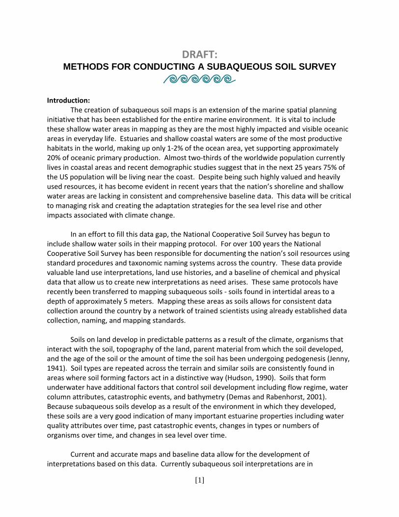
Knowing the area that will be mapped is the first step to determine the time and extent of the work involved. You also need to determine the data set (base map) you will use to make the break from subaerial to subtidal map units and be able to close the soil polygon to an extent. Terrestrial soil surveys should include all coastal and intertidal soil map units. In many cases the coastal areas (dunes, beaches, and tidal marshes) have been mapped but are in need of update mapping to adjust for erosion and deposition of the features.

Figure 1: Left: Published soil survey map for an area in Nantucket, MA (1976), Right 2001 aerial photo of same

area, note the changes of the barrier island spits.

Many older surveys did not map intertidal areas as miscellaneous map units (such as intertidal mud or sand flats) so these areas should be included either as soil units or miscellaneous areas. If you have existing SSURGO data it is recommended this new mapping area be appended to the existing soil polygons to create a seamless map, some adjusting for new ortho-photography may be needed. The decision where to draw the line on the map between the sub-aerial and subaqueous soils is often difficult and depends on the tide the base map photography was flown, it is possible to make the determination once you have completed the bathymetric survey. This decision should be made with consultation with your partners and identified in the work plan. You should also check NOAA Shoreline Map to determine if your area has been mapped by NOAA: http://shoreline.noaa.gov/

For SSURGO data it may be necessary to have the survey area boundary coverage (soils_a_ri600 for example) adjusted to a new boundary to include the submerged lands. This could follow a state water line, a bathymetric cut-off depth (5m for example) or some other break.

[4]

Step 2: Identify Existing data for your Area

this step is similar to terrestrial mapping, review what other scientists and mappers have collected at the site prior to collecting any field data. You may find a wealth of existing bathymetry (NOAA, COE, State, etc.), acoustic data, water quality, sediment and geologic maps, etc. Also it is always good to research imagery for your area, old imagery may provide information about the area and new imagery is usually available from a variety of sources. Assemble all existing data and review it prior to mapping.

Step 3: Creating a Subaqueous Terrain Map (bathymetry and soil landscapes)

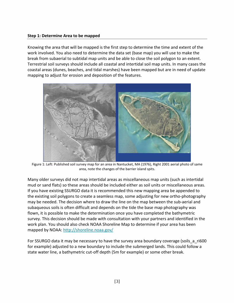
Because of the overlying water, submerged landscapes and landforms cannot be identified easily using standard methods such as stereo photography or visual assessment of the landscape. Therefore, identification and delineation of subaqueous landscape units is somewhat more complicated than that of terrestrial landscapes, and development of subaqueous topographic maps is a critical first step toward delineating subaqueous landscape units.

Figure 2: Oblique aerial photo of Ninigret Pond, Charlestown, RI showing landscape units.

Subaqueous landscape units provided a first approximation of soil distributions and offered an objective delineation of subaqueous soil map units. These landscape units are based on water depth, slope, coastal geologic landforms, and geographic position. Landforms and landscape units such as coves, submerged beaches, shoals, washover fan flats, and slopes are common examples found in many coastal lagoons along the east coast of the United States. These units were defined and described by the Subaqueous Soils Subcommittee (2005). Subaqueous

[5]

landforms are fundamentally the same as those in the subaerial environment and have a discernable topography from which subaqueous landscape units may be identified (Bradley and Stolt, 2003; Subaqueous Soils Subcommittee, 2005). In many areas, these features can be observed using aerial photography and side-scan imagery, but in general, a contour map illustrating the subtidal topography was necessary to define the boundaries of each unit. Information on the glossary developed can be found at: http://nesoil.com/sas/glossary.htm or on the NSSH - ftp://ftp-fc.sc.egov.usda.gov/NSSC/Soil_Survey_Handbook/629_glossary.pdf

The data used to construct such a map are generally bathymetric data (water depths). The water depth data are used to produce a contour map from which subaqueous landforms can be identified and delineated to begin the soil survey. Thus, x, y, and z coordinates are necessary to create a contour map.

XY locations can be accurately measured using a Differential GPS or a GPS with WAAS (Wide Area Augmentation System; http://www8.garmin.com/aboutGPS/waas.html) correction.

Water depths can be determined in a number of ways. The quickest and most cost-effective approach is to use a single beam fathometer or sounder. These devices are sold for navigation and fishing purposes, but provide accurate location (XY) data, as well as depth (Z) and, in many cases, an acoustic image of the subaqueous soil surface and profile. Trackline data can be viewed on the screen of the sounder over nautical charts, and XYZ data is stored in the sounder’s computer. Survey grade multibeam fathometers are also available, which provide a more complete picture of the subaqueous soil surface, however, the abundance of point data requires a significant amount of post-processing. Often expensive third-party software in needed to process the data from survey grade equipment.

Both fathometers use a transducer that is attached to the boat just below the water line. As the boat moves along, water depths are obtained and stored in the fathometer computer or a device such as laptop. Demas and Rabenhorst (1998) reported that soundings were collected at approximately 4 km2/hr.

In tidally influenced waters, tide corrections are made from data collected from tide gauges operating at the same time that the bathymetric data are being collected. One to three tide gauges are generally required depending upon the size of the area of interest and the complexity of the tidal cycle within the estuary. Tide gauges should be surveyed in to determine the exact elevation of the gauge. Tide corrections can be made in a number of ways. Simple tidal fluctuations can be corrected for using Excel or other spreadsheet software. Complex corrections may require use of software designed for the purpose (ie. Hypack 2.12A Gold software).

Data should be reviewed to remove aberrant depths and aberrant XY locations. A number of software programs are available to construct topographic maps. As an example, an ArcView approach is provided here:

[6]

A TIN model was created using the bathymetric soundings and a hard breakline (depth = 0) consisting of the wetline from recent orthophotos. The TIN was converted to a GRID (30 foot pixel size). Land from the orthophoto wetline was used as a mask to set all land-based pixels to NODATA. The bathymetric GRID was smoothed by applying a 3 pixel radius averaging filter and contours were created from the smoothed bathymetric GRID. The data processing can be validated by repeating the processing with fewer points and using the randomly selected points that were removed for statistical comparisons based on residuals.

Using the fathometer from a boat is limited to certain water depths (greater than 45 cm). In areas where there is considerable tidal fluctuation (a meter of more tidal fluctuation), shallow water may be profiled at high tides. If tidal fluctuations are less, surveying of the shallow water may be necessary. This can be done with a survey grade GPS that records elevations (RTK), a total station, or an all-purpose elevation rod and level. This approach can also be used to validate contour maps created from bathymetric data.

In waters with a large amount of submerged aquatic vegetation (SAV), acoustic sounders can provide inaccurate water depth data as they often reflect the top of the thick SAV instead of the true water depth. For this reason, fathometer readings should be periodically verified with manual water depth readings using a stadia rod. In cases where SAV is very thick, manual measurements may have to be the sole source of bathymetry data. In coastal areas where the SAV consists mostly of eelgrass, fathometer data collection during the winter months when eelgrass has died back can provide better results as well.

Bathymetric data is collected relative to NAVD88 in order to produce a seamless terrain model. While NAVD88 is the standard vertical datum in North America, it is a fixed geodetic vertical datum, and as such, does not reflect local variations in sea level between different stations (Rapp, 1994; NGS, 2007). Continuous water level observations, collected over a set period (typically one lunar month that overlaps with bathymetric surveying), are used to calculate the tidal datums (i.e. Mean Lower Low Water (MLLW), Mean Sea-level (MSL), Mean Higher High Water (MHHW) etc.). These datums are determined relative to the stations NAVD88 elevation using the definitions of Voigt (1998) and can be converted to the desired datum (i.e., MLLW) by setting that particular datum to zero. A tidal datum should be considered a local datum, and as such, should not be extended across areas with differing hydrographic characteristics (NOAA, 2003). http://www.esri.com/news/arcuser/0703/geoid1of3.html Bathymetry Process for tidally influenced waters Tide data collection: 1: Deploy tide gauges

-Tide gauges deployed to record water depth every 6 minutes during the time that surveys are being conducted.

[7]

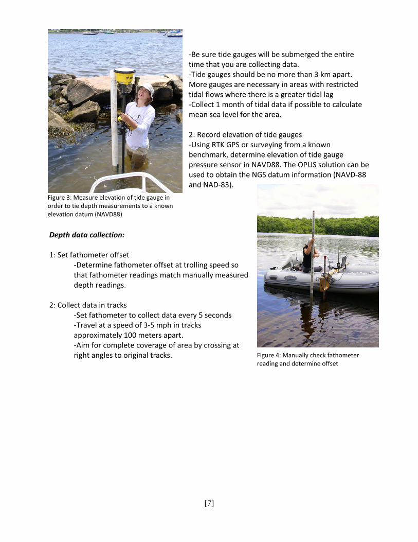
-Be sure tide gauges will be submerged the entire time that you are collecting data. -Tide gauges should be no more than 3 km apart. More gauges are necessary in areas with restricted tidal flows where there is a greater tidal lag -Collect 1 month of tidal data if possible to calculate mean sea level for the area. 2: Record elevation of tide gauges -Using RTK GPS or surveying from a known benchmark, determine elevation of tide gauge pressure sensor in NAVD88. The OPUS solution can be used to obtain the NGS datum information (NAVD-88 and NAD-83).

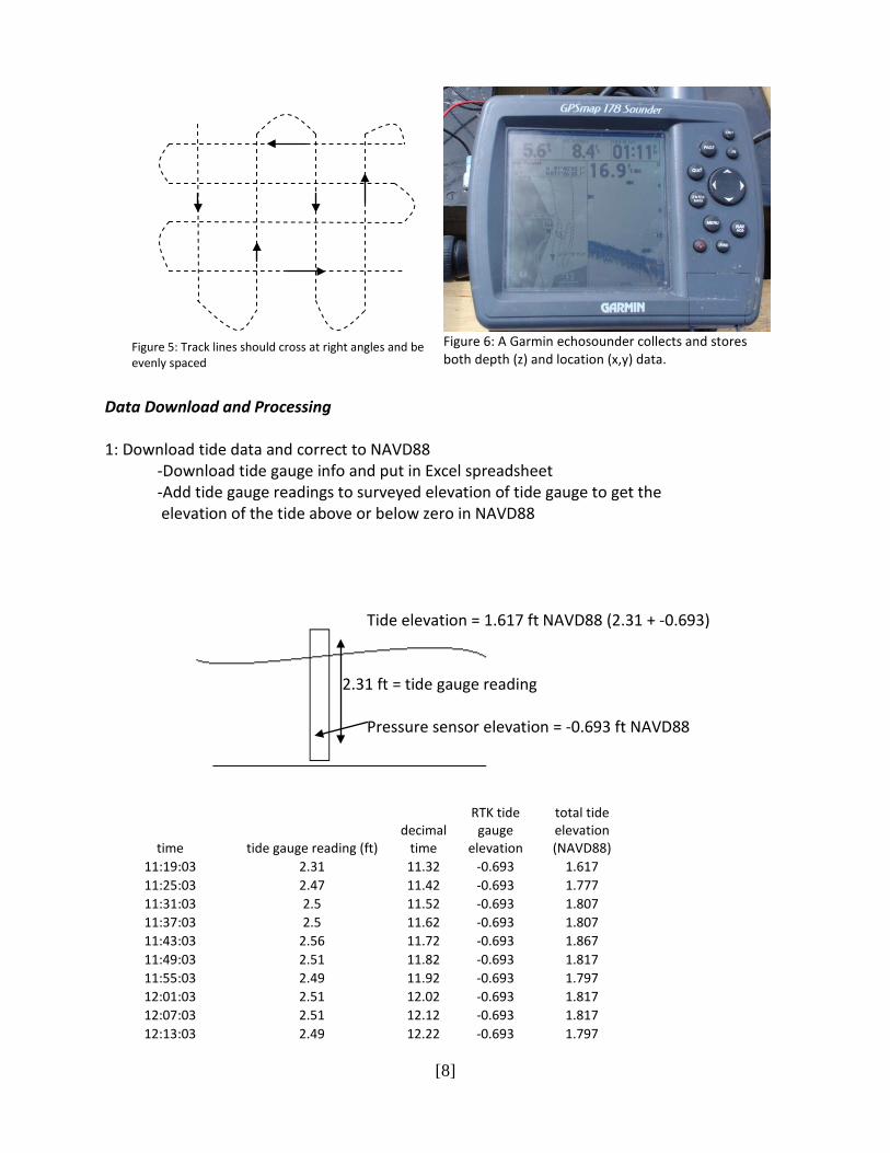
Depth data collection: 1: Set fathometer offset

-Determine fathometer offset at trolling speed so that fathometer readings match manually measured depth readings.

2: Collect data in tracks

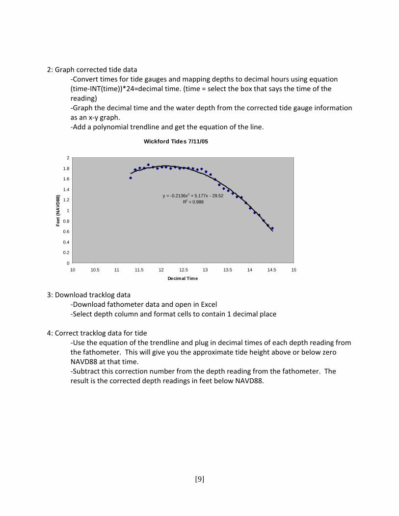
-Set fathometer to collect data every 5 seconds -Travel at a speed of 3-5 mph in tracks approximately 100 meters apart. -Aim for complete coverage of area by crossing at right angles to original tracks.

Figure 3: Measure elevation of tide gauge in order to tie depth measurements to a known elevation datum (NAVD88)

Figure 4: Manually check fathometer reading and determine offset

[8]

Data Download and Processing 1: Download tide data and correct to NAVD88

-Download tide gauge info and put in Excel spreadsheet -Add tide gauge readings to surveyed elevation of tide gauge to get the elevation of the tide above or below zero in NAVD88

Tide elevation = 1.617 ft NAVD88 (2.31 + -0.693)

2.31 ft = tide gauge reading

Pressure sensor elevation = -0.693 ft NAVD88

time tide gauge reading (ft) decimal

time

RTK tide gauge

elevation

total tide elevation (NAVD88)

11:19:03 2.31 11.32 -0.693 1.617 11:25:03 2.47 11.42 -0.693 1.777 11:31:03 2.5 11.52 -0.693 1.807 11:37:03 2.5 11.62 -0.693 1.807 11:43:03 2.56 11.72 -0.693 1.867 11:49:03 2.51 11.82 -0.693 1.817 11:55:03 2.49 11.92 -0.693 1.797 12:01:03 2.51 12.02 -0.693 1.817 12:07:03 2.51 12.12 -0.693 1.817 12:13:03 2.49 12.22 -0.693 1.797

Figure 5: Track lines should cross at right angles and be evenly spaced

Figure 6: A Garmin echosounder collects and stores both depth (z) and location (x,y) data.

[9]

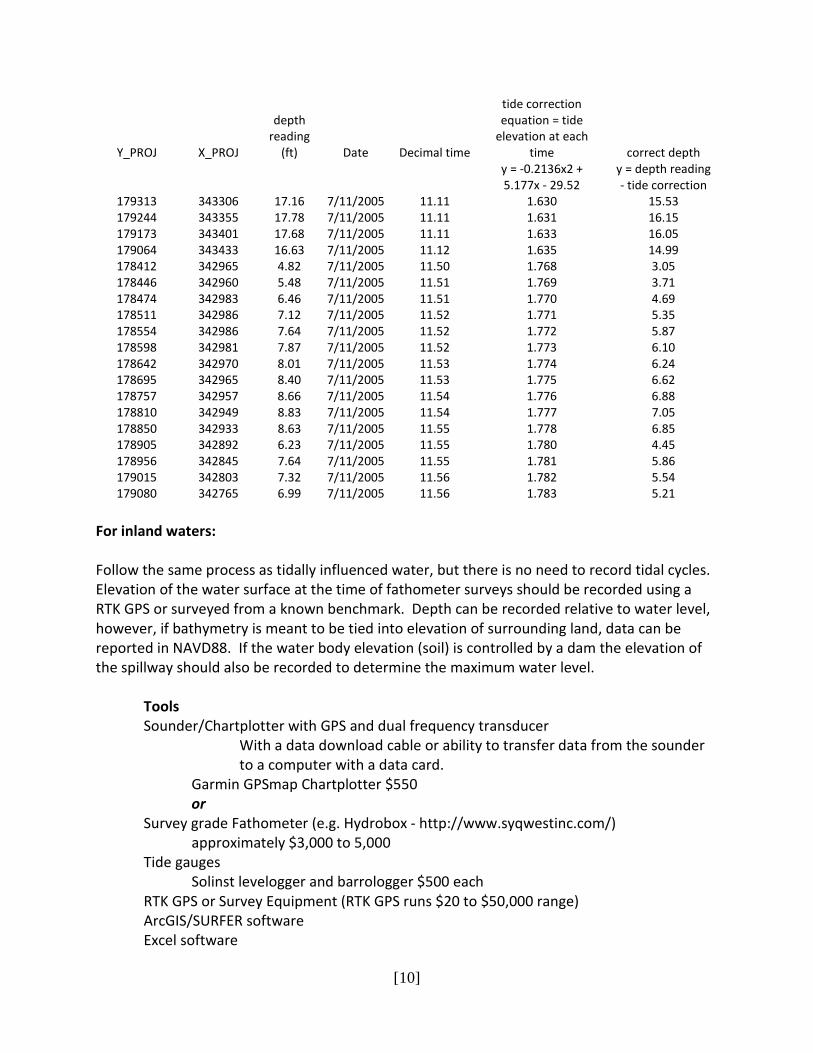
2: Graph corrected tide data

-Convert times for tide gauges and mapping depths to decimal hours using equation (time-INT(time))*24=decimal time. (time = select the box that says the time of the reading) -Graph the decimal time and the water depth from the corrected tide gauge information as an x-y graph. -Add a polynomial trendline and get the equation of the line.

Wickford Tides 7/11/05

y = -0.2136x2 + 5.177x - 29.52R2 = 0.988

0

0.2

0.4

0.6

0.8

1

1.2

1.4

1.6

1.8

2

10 10.5 11 11.5 12 12.5 13 13.5 14 14.5 15

Decimal Time

Feet

(NA

VD88

)

3: Download tracklog data

-Download fathometer data and open in Excel -Select depth column and format cells to contain 1 decimal place

4: Correct tracklog data for tide

-Use the equation of the trendline and plug in decimal times of each depth reading from the fathometer. This will give you the approximate tide height above or below zero NAVD88 at that time. -Subtract this correction number from the depth reading from the fathometer. The result is the corrected depth readings in feet below NAVD88.

[10]

Y_PROJ X_PROJ

depth reading

(ft) Date Decimal time

tide correction equation = tide

elevation at each time correct depth

y = -0.2136x2 + 5.177x - 29.52

y = depth reading - tide correction

179313 343306 17.16 7/11/2005 11.11 1.630 15.53 179244 343355 17.78 7/11/2005 11.11 1.631 16.15 179173 343401 17.68 7/11/2005 11.11 1.633 16.05 179064 343433 16.63 7/11/2005 11.12 1.635 14.99 178412 342965 4.82 7/11/2005 11.50 1.768 3.05 178446 342960 5.48 7/11/2005 11.51 1.769 3.71 178474 342983 6.46 7/11/2005 11.51 1.770 4.69 178511 342986 7.12 7/11/2005 11.52 1.771 5.35 178554 342986 7.64 7/11/2005 11.52 1.772 5.87 178598 342981 7.87 7/11/2005 11.52 1.773 6.10 178642 342970 8.01 7/11/2005 11.53 1.774 6.24 178695 342965 8.40 7/11/2005 11.53 1.775 6.62 178757 342957 8.66 7/11/2005 11.54 1.776 6.88 178810 342949 8.83 7/11/2005 11.54 1.777 7.05 178850 342933 8.63 7/11/2005 11.55 1.778 6.85 178905 342892 6.23 7/11/2005 11.55 1.780 4.45 178956 342845 7.64 7/11/2005 11.55 1.781 5.86 179015 342803 7.32 7/11/2005 11.56 1.782 5.54 179080 342765 6.99 7/11/2005 11.56 1.783 5.21

For inland waters: Follow the same process as tidally influenced water, but there is no need to record tidal cycles. Elevation of the water surface at the time of fathometer surveys should be recorded using a RTK GPS or surveyed from a known benchmark. Depth can be recorded relative to water level, however, if bathymetry is meant to be tied into elevation of surrounding land, data can be reported in NAVD88. If the water body elevation (soil) is controlled by a dam the elevation of the spillway should also be recorded to determine the maximum water level.

Tools Sounder/Chartplotter with GPS and dual frequency transducer

With a data download cable or ability to transfer data from the sounder to a computer with a data card.

Garmin GPSmap Chartplotter $550 or

Survey grade Fathometer (e.g. Hydrobox - http://www.syqwestinc.com/) approximately $3,000 to 5,000

Tide gauges Solinst levelogger and barrologger $500 each

RTK GPS or Survey Equipment (RTK GPS runs $20 to $50,000 range) ArcGIS/SURFER software Excel software

[11]

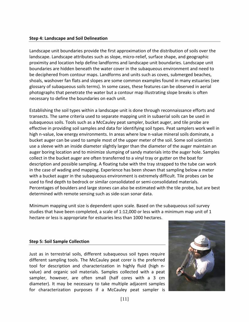
Step 4: Landscape and Soil Delineation Landscape unit boundaries provide the first approximation of the distribution of soils over the landscape. Landscape attributes such as slope, micro-relief, surface shape, and geographic proximity and location help define landforms and landscape unit boundaries. Landscape unit boundaries are hidden beneath the water cover in the subaqueous environment and need to be deciphered from contour maps. Landforms and units such as coves, submerged beaches, shoals, washover fan flats and slopes are some common examples found in many estuaries (see glossary of subaqueous soils terms). In some cases, these features can be observed in aerial photographs that penetrate the water but a contour map illustrating slope breaks is often necessary to define the boundaries on each unit. Establishing the soil types within a landscape unit is done through reconnaissance efforts and transects. The same criteria used to separate mapping unit in subaerial soils can be used in subaqueous soils. Tools such as a McCauley peat sampler, bucket auger, and tile probe are effective in providing soil samples and data for identifying soil types. Peat samplers work well in high n-value, low energy environments. In areas where low n-value mineral soils dominate, a bucket auger can be used to sample most of the upper meter of the soil. Some soil scientists use a sleeve with an inside diameter slightly larger than the diameter of the auger maintain an auger boring location and to minimize slumping of sandy materials into the auger hole. Samples collect in the bucket auger are often transferred to a vinyl tray or gutter on the boat for description and possible sampling. A floating tube with the tray strapped to the tube can work in the case of wading and mapping. Experience has been shown that sampling below a meter with a bucket auger in the subaqueous environment is extremely difficult. Tile probes can be used to find depth to bedrock or similar consolidated or semi-consolidated materials. Percentages of boulders and large stones can also be estimated with the tile probe, but are best determined with remote sensing such as side-scan sonar data. Minimum mapping unit size is dependent upon scale. Based on the subaqueous soil survey studies that have been completed, a scale of 1:12,000 or less with a minimum map unit of 1 hectare or less is appropriate for estuaries less than 1000 hectares. Step 5: Soil Sample Collection Just as in terrestrial soils, different subaqueous soil types require different sampling tools. The McCauley peat corer is the preferred tool for description and characterization in highly fluid (high n-value) and organic soil materials. Samples collected with a peat sampler, however, are often small (half cores with a 3 cm diameter). It may be necessary to take multiple adjacent samples for characterization purposes if a McCauley peat sampler is

[12]

employed because materials with a high n-value often has a small dry mass. High n-value materials can also be collected in a core barrel using a piston sampler. This type of sampler is an open tube or core barrel with a rubber plug inside the barrel that rises up as the barrel is pushed into the soil. The plug maintains a short, nearly air-tight space just above the sample to minimize disturbance, while the suction minimizes compaction. Bucket augers are used for collecting field note descriptions, transects, and field mapping in areas of non-fluid soils (sandy to gravelly areas) and for locating areas for collecting full vibra-core samples. Using a bucket auger in shallow water can be extremely labor intensive and is generally limited to coring to approximately 50 to 70 cm, below this depth suction makes retrieving the sample difficult. For both of the traditional hand tools above it is useful to have multiple extensions available for the various water depths. The best type to use are the augers that have the “quick release” system rather than the threaded screw systems as these become difficult to add extensions and often freeze up with rust. If available stainless augers will last longer but are more expensive. A 4 inch diameter regular bucket auger works best but having several auger types is also helpful along with a dutch auger. For the McCauley a 50 cm length blade works well but a 1 m blade, while a lot heavier, will cut the number of samples needed in half. Another useful tool is to have two rubber rings on each extension (a garden hose gasket works fine). These are used to slide to the water level to mark your current depth, this will help determine you next sampling interval for a complete sample. Vibracoring: Vibracore sampling is the most effective approach to obtain minimally disturbed samples of less fluid material for detailed description and sampling of typical pedons. A vibracore rig consists of an engine (minimum 5.5 hp, best is 8 hp), a cable, and vibrating head (2.5 in or bigger). The engine creates a high frequency, low amplitude vibration. The vibration is transferred through a cable to the vibracore head that is bolted to the top of core barrel or tube. These vibrators are made for vibrating concrete for removing bubbles before setting. The vibration essentially liquefies the soil materials, enabling the core barrel to penetrate into the soil materials. Core barrels are generally made out of 7.5 to 10 cm inside diameter aluminum pipe (irrigation pipe). Some barrels are made out of polycarbonate (these are clear and light, but also 6 to 7 times more expensive than aluminum). Core barrel lengths should be as long as the soil to be sampled, plus water depth, and an extra 50 or 60 cm. Sources of core barrels may be found from irrigation supply companies, another potential source is to talk with your NRCS planners and engineers to see if they know of farms that have them stockpiled and available to buy. Many farms are switching from aluminum to plastic irrigation and are looking to scrap their old tubes. Prices for new tubes runs $2-3/foot, best o buy in 30 foot sections and cut in half for use.

[13]

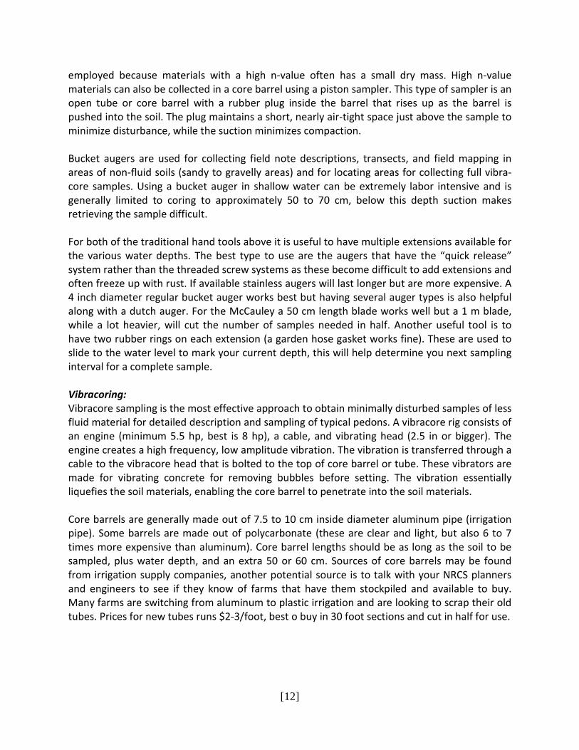
The vibracore head is bolted to the core using either heavy-duty U-bolts or a custom welded fitting. The attachment must be very secure, as the vibration tends to loosen bolts and cause slippage if not properly tightened. Vibracore heads are usually custom made by a fabricator, depending on the boat platform you will either need to have a head that runs parallel to the core (if moon-pool space is limited) or perpendicular if you have more space, the later setup appears to create the strongest vibrations and works best. If no head is available attaching the head directly to the barrel using u-clamps works but often comes loose and dents the barrel.

Step by Step Procedure: Step 1: Preparation - Define the area to be cored, select the best location for the map unit,

determine proper tide conditions (outgoing or low tide for deep areas, high tide for shallows). A checklist of equipment needed for the coring day is highly recommended; forgetting one piece of equipment can cause delays. Extra equipment and tools should be brought along as dropping stuff overboard is inevitable. A heavy duty magnet is good to have onboard along with diving equipment in case equipment is dropped overboard.

Step 2: Secure Vessel – Once you are at the site to be cored you must get the coring vessel secured so it will not move. There are several ways to keep the boat from drifting around; first is to have the boat face the wind or flowing water direction. Two bow anchors are needed to be dropped in a Y-pattern and a stern anchor set. Keeping the engine in reverse also works well if no stern anchor is available. Other options are to use steel rods drilled into the soil from the bow and stern or have a person in the water holding the boat still.

Step 3: Core Preparation – Once the vessel is secure mark the waypoint location with a GPS and determine the water elevation (depth) with a survey rod. The core should then be cut to the proper length to allow the proper amount of soils to be sampled, an additional 5-7 feet of core barrel should be added for core settlement, tide changes, and to have some of the core above the water for retrieval. Once the core barrel is cut it should be measured and the total length noted on the core form.

Step 4: Coring – Once the core is attached to the core head and you are ready to begin the vital next step is SAFTEY. Anyone on board the vessel needs to have a hard hat, gloves, shoes (no open toes), and is paying attention to the coring operation. The core barrel and head are inserted into the moon pool and positioned straight. The engine operator then turns on the engine and the core is vibrated into the soil. In some cases the vibracoring may require weight to be applied to get through some soil layers. People may need to

Figure 7: A vibracore set up using a tripod and chain-fall to extract a core through the “moon pool” of a pontoon boat.

[14]

stand on the head and top of core or pull ropes down. If the core won’t budge any deeper turn off the engine and note refusal on the log.

Step 5: Retrieving the Core - Once a core is vibrated into the soil to a satisfactory depth, the amount of soil compaction (referred to as “core rot”) within the core is measured, this is done to be able to provide corrections for depths to layers and bulk density measurements. This is done by measuring the length from the top of the core barrel to the soil surface outside of the core as well as inside the core using a sinker attached to a rope. The difference in length is the amount of compaction or settling that occurred in the sample during vibracoring. See the log sheet at end of this document. Once these measurements are made it is time to pull the core. The core barrel is filled to the top with water and a cap is screwed to the top as tight as possible to create suction. Pulling the core out of the soil is done using either a chain-fall or a power winch, using a come-along is not recommended. Make sure your straps are strong enough to pull the cores out. Once the core is almost out of the soil a person with a bottom cap needs to be ready to quickly seal the bottom of the core as the final section is pulled onto the boat. Remove the vibracore head assembly.

Step 6: Completing the core – Once the core is on the deck of the boat and the bottom cap is duct taped shut, the core is ready to be cut. Place the weighted string into the core to determine the soil surface and mark that level on the core. Using a large pipe-cutter or hack saw cut the barrel a few inches above the soil surface – use caution when cutting the core, one person needs to grab the top section and one the bottom, gloves should be worn as the cores are very sharp. Once cut place something in the core to protect the surface (a “whacky noodle” works best) and attach the top cap and duct tape it shut. Using a sharpie label the core with the pedon ID, Waypoint, date, and an arrow indicating the surface. Cores are then stored upright on board the sampling vessel and then transferred to cold storage (4C). Cores are kept refrigerated until they can be opened and sampled.

Tools/Sources: 5.5 HP. GAS VIBRATOR - 14 FT. SHAFT - 2-1/2" HEAD $2,500 (2007) http://www.improvedconstructionmethods.com/dreyer_gasoline_concrete_vibrators.htm Tripod (search rescue tripod in Internet) $1,290 Chain fall $250 Plastic caps for cores (EC-64?) http://www.caplugs.com List of Equipment Used: Engine and Shaft Straps Sharpie Vibracore head Core catcher Duct Tape (lots) Tripod Bolts and nuts (spares) Screw Cap Chainfall \ Power Winch Hard Hats Core barrels Bucket for water Caps (two per core) GPS Survey Rod Anchors (3) First aid kits

[15]

Example of Vibracore Log Sheet:

[16]

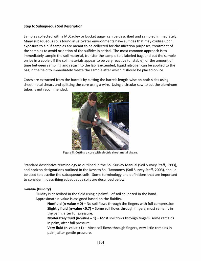
Step 6: Subaqueous Soil Description Samples collected with a McCauley or bucket auger can be described and sampled immediately. Many subaqueous soils found in saltwater environments have sulfides that may oxidize upon exposure to air. If samples are meant to be collected for classification purposes, treatment of the samples to avoid oxidation of the sulfides is critical. The most common approach is to immediately sample the soil material, transfer the sample to a labeled bag, and put the sample on ice in a cooler. If the soil materials appear to be very reactive (unstable), or the amount of time between sampling and return to the lab is extended, liquid nitrogen can be applied to the bag in the field to immediately freeze the sample after which it should be placed on ice. Cores are extracted from the barrels by cutting the barrels length-wise on both sides using sheet metal shears and splitting the core using a wire. Using a circular saw to cut the aluminum tubes is not recommended.

Figure 8: Cutting a core with electric sheet metal shears.

Standard descriptive terminology as outlined in the Soil Survey Manual (Soil Survey Staff, 1993), and horizon designations outlined in the Keys to Soil Taxonomy (Soil Survey Staff, 2003), should be used to describe the subaqueous soils. Some terminology and definitions that are important to consider in describing subaqueous soils are described below. n-value (fluidity)

Fluidity is described in the field using a palmful of soil squeezed in the hand. Approximate n-value is assigned based on the fluidity.

Nonfluid (n-value = 0) – No soil flows through the fingers with full compression Slightly fluid (n-value <0.7) – Some soil flows through fingers, most remains in the palm, after full pressure. Moderately fluid (n-value = 1) – Most soil flows through fingers, some remains in palm, after full pressure. Very fluid (n-value >1) – Most soil flows through fingers, very little remains in palm, after gentle pressure.

[17]

Odor Sulfide odor is described as strong, moderate, weak, or none immediately after soil is exposed to air.

Reaction to hydrogen peroxide Sulfidic materials accumulate within a soil that is permanently saturated, generally with brackish water. The sulfates in the water are biologically reduced to sulfides as the materials accumulate. Sufidic materials commonly accumulate in coastal marshes near the mouth of rivers that carry noncalcareous sediments, but they may occur in freshwater marshes if there is sulfur in the water. Monosulfides, often in the form of Fe(II) monosulfides, are visible in reduced soil as a dark black color. When a sulfidic soil is oxidized, either in place due to oxidized water conditions, or when the soil is drained, Fe(III) is formed, and the typical black color is lost, leaving a gray or brown color (Lyle, 1983). An example of a common monosulfide oxidation reaction:

FeS + O2 + H2O = Fe(OH)3 + H+ + SO4 Sulfidic materials are typically determined in the laboratory using incubation pH measurement in which a soil is kept in incubation for 8 weeks and the initial and final pH measurements are made. Hydrogen peroxide has also been used in determination of the presence of reduced sulfides in soil samples with pH measurements made after complete oxidation with H2O2 (Finkelman and Giffin, 1986; Jennings et al., 1999). Hydrogen peroxide speeds up the natural oxidation reaction and can be represented in the following reaction:

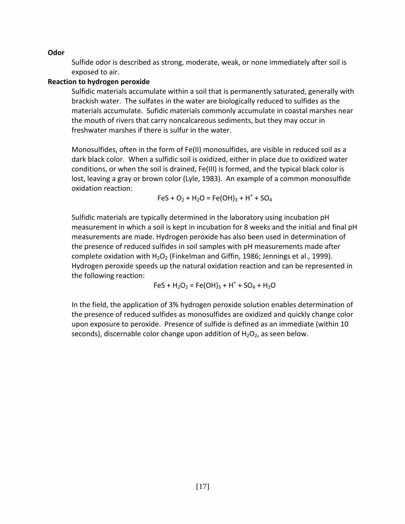
FeS + H2O2 = Fe(OH)3 + H+ + SO4 + H2O In the field, the application of 3% hydrogen peroxide solution enables determination of the presence of reduced sulfides as monosulfides are oxidized and quickly change color upon exposure to peroxide. Presence of sulfide is defined as an immediate (within 10 seconds), discernable color change upon addition of H2O2, as seen below.

[18]

Figure 9: Applying hydrogen peroxide to a reduced soil

Horizon Designations:

A horizons: “Mineral horizons that formed at the surface or below an O horizon, that exhibit obliteration of all or much of the original rock structure, and that show one or more of the following: (1) an accumulation of humified organic matter intimately mixed with the mineral fraction and not dominated by properties characteristic of E or B horizons (defined below) or (2) properties resulting from cultivation, pasturing, or similar kinds of disturbance.” (Soil Survey Staff, 1993)

Subaqueous soils are often described with an A horizon at the surface if that horizon shows a darker color due to an accumulation of organic matter. Some subaqueous soils are described without an A horizon if there is no obvious accumulation of organic matter such as in a very active flood tidal delta landform. Buried A horizons (Ab) are commonly described when a soil is interpreted to have had a stable surface long enough to accumulate organic matter, and was subsequently buried with mineral material. These horizons are identified by a darker color.

B horizons: “Horizons that formed below an A, E,, or O horizon and are dominated by obliteration of all or much of the original rock structure and show one or more of the following:

1. illuvial concentration of silicate clay, iron, aluminum, humus, carbonates, gypsum, or

silica, alone or in combination;

2. evidence of removal of carbonates;

[19]

3. residual concentration of sesquioxides;

4. coatings of sesquioxides that make the horizon conspicuously lower in value, higher in

chroma, or redder in hue than overlying and underlying horizons without apparent

illuviation of iron;

5. alteration that forms silicate clay or liberates oxides or both and that forms granular,

blocky, or prismatic structure if volume changes accompany changes in moisture

content; or

6. brittleness.” (Soil Survey Staff, 1993)

Subaqueous soils very rarely are described with B horizons. In cases where a submerged soil is present, a B horizon may be described within the buried soil profile.

C horizons or layers: “Horizons or layers, excluding hard bedrock, that are little affected by pedogenic processes and lack properties of O, A, E, or B horizons. The material of C layers may be either like or unlike that from which the solum presumably formed. The C horizon may have been modified even if there is no evidence of pedogenesis.” (Soil Survey Staff, 1993)

Transitional Horizons: AC and CA horizons are described in subaqueous soils. These transitional horizons are formed between surface A horizons and subsurface C horizons and have qualities of both master horizons.

g Strong gleying: “This symbol is used to indicate either that iron has been reduced and removed during soil formation or that saturation with stagnant water has preserved a reduced state. Most of the affected layers have chroma of 2 or less and many have redox concentrations. The low chroma can be the color of reduced iron or the color of uncoated sand and silt particles from which iron has been removed.” (Soil Survey Staff, 1993)

The subscript g is used in subaqueous soils for those horizons with a value of 4 or more moist or 6 or more dry and a chroma of 2 or less.

Use of discontinuity: “A discontinuity is a significant change in particle-size distribution or mineralogy that indicates a difference in the material from which the horizons formed and/or a significant difference in age, unless that difference in age is indicated by the suffix "b." Symbols to identify discontinuities are used only when they will contribute substantially to the reader's understanding of relationships among horizons. Stratification common to soils formed in alluvium is not designated as discontinuity, unless particle size distribution differs markedly (strongly contrasting particle-size class, as defined by Soil Taxonomy) from layer to layer even though genetic horizons have formed in the contrasting layers.” (Soil Survey Staff, 1993) Discontinuities in subaqueous soils are described when there is a significant change in particle-size that indicates that the material was deposited by a different process. Important examples are a discontinuity at the change from material deposited in a marine environment to older

[20]

material deposited on land and later inundated. Deposits of similar particle size from multiple overwash events behind a barrier are not described as discontinuities. si-sulfidic (proposed subordinate distinction – 2010): This symbol indicates the presence of sulfides in mineral or organic horizons. Sulfidic horizons typically have dark colors; values <4, and chromas <2. These horizons typically form in coastal environments that are permanently saturated (tidal marshes or estuarine subaqueous soils) and have a source of sulfur to form sulfides. Such horizons may have a sulfidic odor when first exposed to air. Sulfidic horizons may also be geologic in origin. Examples include coal deposits or coastal plain deposits such as glauconite that have not been oxidized because of thick overburden. Step 7: Soil Sample Analysis Most sample analysis for subaqueous soils can be made following standard procedures outlined in the Soil Survey Laboratory Methods Manual (Soil Survey Staff, 2004). Certain soil properties will be affected by the subaqueous environment and laboratory procedures should be conducted with this in mind. Sulfides, salts, and shell fragments are the most important to consider when analyzing the soil and are worth noting. The presence of sulfides in the soils has been noted above and should be accommodated. Measurements of sulfides are not well documented in soil survey publications. Thus, if this characteristic is to be measured consideration should be given to the numerous methods to measure chromium reducible and acid volatile sulfides. Particle size distribution analysis may need to be altered to accommodate for the weight and flocculation capability of salts. Samples can be washed to remove salts using dialysis tubing. Carbonates in shell fragments can be an issue in measuring organic carbon and should be considered when organic and inorganic carbon is being determined.

A. Particle Size Particle size is conducted in the standard Soil Survey Laboratory method (3A1a1;

Soil Survey Staff, 2004), being sure to pretreat for the removal of organic matter and soluble salts that can impact dispersion.

B. Organic Carbon and Inorganic Carbon Total organic carbon and calcium carbonate can be determined sequentially by percent weight loss on ignition (LOI) assuming organic matter combustion at 550 °C and a soil organic carbon-organic matter ratio of 0.5 (Nelson and Sommers, 1996). Calcium carbonate can be determined by loss on ignition at 1000 ˚C calculated as:

CaCO3 = (DW550-DW1000)/0.5995 where CaCO3 is the weight of the calcium carbonate in the original sample, DW550 is the dry weight after LOI at 550 ˚C, DW1000 is the dry weight after combustion at 1000 ˚C, and

[21]

0.5995 represents the percent of CaCO3 that is lost as carbon dioxide through combustion (Heiri et al., 2001). C. Incubation pH Soil pH was is measured initially after sampling or thawing a frozen sample using a pH probe. Samples are mixed with equal parts soil and water. Samples are incubated in open beakers at room temperature for 16 weeks with water added weekly to maintain moist conditions.

D. Electrical Conductivity (5:1 method)

Electrical conductivity is measured on samples that have been stored in the freezer immediately after sampling. One part soil to five parts DI water by volume are mixed in a beaker. Electrical conductivity is measured using a hand-held conductivity meter. E. Bulk Density Bulk density measurements are calculated based on the dried weight of a known volume of soil at the field moisture status. For samples taken as vibracores and opened by cutting, a 50 ml syringe with the end removed is used as a mini-core to sample a 10 ml volume sample. Samples collected in a peat sampler can be analyzed for bulk density if a known volume is sampled and dried. F. Sulfides

Sulfide extraction can be done according to the diffusion method in which sulfides are trapped in a sulfide antioxidant buffer (SAOB) (Fossing and Jorgensen, 1989; Brouwer and Murphy, 1994; Ulrich et al., 1997; Boothman, 1998; Bradley and Stolt, 2006). One gram of frozen soil is added to 150 ml serum bottles that contained a 10 x 75 mm vial containing 3 ml SAOB. Bottles are immediately filled with N2 gas and stoppered. A second set of samples are weighed and dried overnight in a 105 ˚C oven to determine dry weight. Soils are reacted with 12 ml of O2-free 2N HCl added with a syringe to the sample bottle. Bottles are rotated for one hour at 150 rpm, after which SAOB traps are removed for analysis. A second SAOB trap is inserted into the same bottle. The bottle is purged of O2 with N2 gas and reacted with 4 ml of O2-free 12N HCl and eight ml of Cr2+ added with a syringe. The Cr2+ solution is prepared by adding 1M CrCl3·H2O in 0.5N HCl to a modified Jones Reductor built from a separatory funnel filled with mossy Zinc and a glass wool filter (Fossing and Jorgensen, 1989). Bottles are rotated at 150 rpm for 20 hours and SAOB traps are removed for CRS analysis. Concentrations of AVS and CRS in the SAOB traps are determined using a silver/sulfide ion specific electrode standardized to known concentrations of sulfide in Na2S·9H2O and SAOB solutions (Thermo Electron, 2003). Sulfide concentrations are determined as μg sulfide per g dry soil.

[22]

Sources of exisitng data: http://coastalmap.marine.usgs.gov/ArcIms/Website/usa/eastcoast/atlanticcoast/viewer.htm Trimble Hydrographic - Bathy: http://www.trimble.com/mr_hydrographic.html Bradley Stolt: http://soil.scijournals.org/cgi/content/abstract/67/5/1487 NOAA CSC Lidar: http://www.csc.noaa.gov/crs/rs_apps/sensors/lidar.htm Glossary of coastal terms: http://www.csc.noaa.gov/text/glossary.html Geotech core analyser??: http://www.geotek.co.uk/site/scripts/module.php?webSubSectionID=26 Geodas Data: http://www.ngdc.noaa.gov/mgg/gdas/ LIDAR: http://proceedings.esri.com/library/userconf/proc02/pap0580/p0580.htm ERF: http://www.erf.org/ Coastal america: http://www.coastalamerica.gov/ References: Boothman, W.S. 1998. Determination of degree of pyritization (DOP) in sediments.

Environmnetal Protection Agency, National Health and Ecological Effects Research Laboratory, Atlantic Ecology Division, Narragansett, RI.

Bradley, M.P., and M.H. Stolt. 2003. Subaqueous soil-landscape relationships in a Rhode Island estuary. Soil Science Society of America Journal 67:1487-1495. Bradley, M.P., and M.H. Stolt. 2006. Landscape-level seagrass-sediment relations in a coastal

lagoon. Aquatic Botany 84:121-128. Brouwer, H., and T.P. Murphy. 1994. Diffusion method for the determination of acid-volatile

sulfides (AVS) in sediment. Environmental Toxicology and Chemistry 13:1273–1275. Demas, G.P., and M.C. Rabenhorst. 1999. Subaqueous soils: pedogenesis in a submersed environment. Soil Science Society of America Journal 63:1250-1257. Demas, G.P., and M.C. Rabenhorst. 2001. Factors of subaqueous soil formation; a system of

qualitative pedology for submersed environments. Geoderma 102:189-204. Fossing, H., and B.B. Jorgensen. 1989. Measurement of bacterial sulfate reduction in sediments:

evaluation of a single-step chromium reduction method. Biogeochemistry 8:205-222. Heiri, O., A.F. Lotter, and G. Lemeke. 2001. Loss on ignition as a method for estimating organic

and carbonate content in sediments: reproducibility and comparability of results. Journal of Paleolimnology 25:101-110.

Hudson, B.D. 1990. Concepts of soil mapping and interpretation. Soil Survey Horizons 31:63-73.

[23]

Jenny, H. 1941. Factors of soil formation. McGraw Hill Book Co. Inc., New York, NY. Nelson, D.W., and L.E. Sommers. 1996. Total carbon, organic carbon and organic matter. p. 961-

1010. In Sparks, D.L., A.L. Page, P.A. Helmke, R.H. Loeppert, P.N. Soltanpour, M.A. Tabatabai, C.T. Johnston, and M.E. Sumner (eds.).

Pruett, C. 2010. Developing subaqueous soil interpretations for Rhode Island estuaries: focus

on eelgrass restoration, soil organic carbon pools, and metal pollution. University of Rhode Island Department of Natural Resources Science Master’s Thesis.

Salisbury, A. 2010. Developing subaqueous soil interpretations for Rhode Island estuaries: focus

on shellfish and dredged material placement. University of Rhode Island Department of Natural Resources Science Master’s Thesis.

Soil Survey Staff. 1993. Soil survey manual. Agricultural Handbook No. 18, USDA-NRCS, U.S.

Government Printing Office, Washington, D.C. Soil Survey Laboratory Staff. 2004. Soil survey laboratory methods manual. Soil survey

investigation report no. 42 version 4.0. Unites States Department of Agriculture, Government Printing Office, Washington, D.C.

Thermo-electron. 2003. Orion Silver/Sulfide Electrode Instruction Manual. Thermo-Electron

Corporation, Beverly, MA, USA. Ulrich, G.A., L.R. Krumholz, and J.M. Sulfita. 1997. A rapid and simple method for estimating

sulfate reduction activity and quantifying inorganic sulfides. Applied and Environmental Microbiology 63:1627-1630.