fractional-order control: theory and applications...

Fractional-Order Control: Theory and Applications in Motion Control

by Chengbin Maand Yoichi Hori

Past and Present

The concept of fractional-ordercontrol (FOC) means controlledsystems and/or controllers are

described by fractional-order differen-tial equations. Expanding derivativesand integrals to fractional orders is byno means new and actually has a firmand long-standing theoretical founda-tion. Interest in this subject was evi-dent almost as soon as the ideas ofclassical calculus were known. The ear-liest more or less systematic studiesseem to have been made in the begin-ning and middle of the 19th century byLiouville, Holmgren, and Riemann,although Eular, Lagrange, and othersmade contribution even earlier [1]. Par-allel to these theoretical beginningswas the development of applying frac-tional calculus to various problems [1].

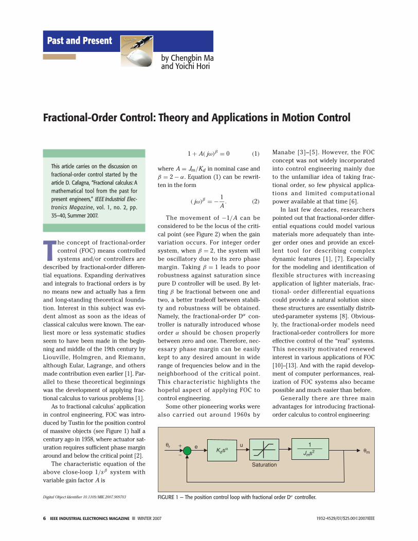
As to fractional calculus’ applicationin control engineering, FOC was intro-duced by Tustin for the position controlof massive objects (see Figure 1) half acentury ago in 1958, where actuator sat-uration requires sufficient phase marginaround and below the critical point [2].

The characteristic equation of theabove close-loop 1/sβ system withvariable gain factor A is

1 + A( jω)β = 0 (1)

where A = Jm/Kd in nominal case andβ = 2 − α. Equation (1) can be rewrit-ten in the form

( jω)β = − 1A

. (2)

The movement of −1/A can beconsidered to be the locus of the criti-cal point (see Figure 2) when the gainvariation occurs. For integer ordersystem, when β = 2, the system willbe oscillatory due to its zero phasemargin. Taking β = 1 leads to poorrobustness against saturation sincepure D controller will be used. By let-ting β be fractional between one andtwo, a better tradeoff between stabili-ty and robustness will be obtained.Namely, the fractional-order Dα con-troller is naturally introduced whoseorder α should be chosen properlybetween zero and one. Therefore, nec-essary phase margin can be easilykept to any desired amount in widerange of frequencies below and in theneighborhood of the critical point.This characteristic highlights thehopeful aspect of applying FOC tocontrol engineering.

Some other pioneering works werealso carried out around 1960s by

Manabe [3]–[5]. However, the FOCconcept was not widely incorporatedinto control engineering mainly dueto the unfamiliar idea of taking frac-tional order, so few physical applica-tions and limited computationalpower available at that time [6].

In last few decades, researcherspointed out that fractional-order differ-ential equations could model variousmaterials more adequately than inte-ger order ones and provide an excel-lent tool for describing complexdynamic features [1], [7]. Especiallyfor the modeling and identification offlexible structures with increasingapplication of lighter materials, frac-tional- order differential equationscould provide a natural solution sincethese structures are essentially distrib-uted-parameter systems [8]. Obvious-ly, the fractional-order models needfractional-order controllers for moreeffective control of the “real” systems.This necessity motivated renewedinterest in various applications of FOC[10]–[13]. And with the rapid develop-ment of computer performances, real-ization of FOC systems also becamepossible and much easier than before.

Generally there are three mainadvantages for introducing fractional-order calculus to control engineering:

Digital Object Identifier 10.1109/MIE.2007.909703

This article carries on the discussion onfractional-order control started by thearticle D. Cafagna, “Fractional calculus: Amathematical tool from the past forpresent engineers,” IEEE Industrial Elec-tronics Magazine, vol. 1, no. 2, pp.35–40, Summer 2007.

1932-4529/07/$25.00©2007IEEE

FIGURE 1 — The position control loop with fractional order Dα controller.

1+

−

θrθm

Saturation

e uKdsα

Jms2

6 IEEE INDUSTRIAL ELECTRONICS MAGAZINE ■ WINTER 2007

1) adequate modeling of controlplant’s dynamic features

2) effective and clear-cut robust con-trol design

3) reasonable realization by approxi-mation.In following sections, detailed

descriptions of the above three advan-tages will be given.

Mathematical Aspects

Mathematic DefinitionsOne of the most frequently encountereddefinitions of fractional-order calculus iscalled the Grünwald-Letnikov definition:

aDαt = lim

h→0nh = t−α

h−αn∑

j=0

(−1) j(

α

j

)

× f(t − jh) (3)

where (

α

j

)are the binomial coeffi-

cients. Obviously, introducing the frac-tional-order calculus leads to infinitedimension, while the integral calculusis finite dimension.

Another widely known definition iscalled the Riemann-Liouville definitionwith an integrodifferential expression.The definition for the fractional-orderintegral is

aD−αt f(t) = 1

�(α)

∫ t

a(t − ξ)α−1

× f(ξ)dξ (4)

while the definition of fractional-orderderivatives is

aDαt f(t) = dγ

dtγ

[aD−(γ−α)

t

](5)

where �(x) is the Gamma function, aand t are limits, and α (α > 0 andα ∈ R) is the order of the operation. γ isan integer that satisfies γ − 1 < α ≤ γ .The Grünwald-Letnikov and Riemann-Liouville definitions are both a unifica-tion of integer order derivatives andintegrals [7].

Laplace and Fourier TransformsFractional-order calculus is quite com-plicated in time domain, as shown inits two definitions. Fortunately one ofthe features most important to controlengineers, its Laplace transform, is

very straightforward [7]. The finalexpression of the Laplace transform ofthe fractional-order derivative is

L{

0Dαt f(t)

} = sα F (s)

−n−1∑k=0

sk0Dα−k−1

t f (0)

(6)

where n − 1 < α < n again. If all theinitial conditions are zero, the Laplacetransform of fractional-order derivativeis simply

L{

0Dαt f(t)

} = sα F (s). (7)

Therefore the Laplace transforms offractional ±α order calculus lead tothe use of fractional-order Laplaceoperator s±α . The transfer functions ofmodels and controllers, which aredescribed by fractional-order differen-tial equations, can be derived conve-niently using fractional-order Laplaceoperator s±α .

Similarly, the Fourier transform offractional-order derivative is

Fe{

0Dαt f(t)

} = ( jω)α F ( jω). (8)

The frequency response of FOC sys-tem can be exactly obtained by substi-tuting s±α with ( jω)±α in its transferfunction. This advantage implies fre-quency-domain analysis of FOC systemis as convenient as integer order con-trol (IOC) systems. The graphical toolsfor IOC in frequency domain are stillavailable for FOC analysis and design.

Modeling and IdentificationRecently, there has been a growing sig-nificant demand for better mathematic

models to describe real objects. Thefractional-order model can provide anew possibility to acquire more ade-quate modeling of dynamic processes.Fractional-order models have beenapplied to describe reheating furnaces[7], viscoelasticity [1], [7], [8], chemicalprocesses [14], and chaos systems [15].

Actually, using a fractional-ordermodel for describing distributed-parameter systems is quite naturalsince the Laplace transform of partialdifferential equations will inevitablyintroduce the fractional-order s opera-tor. For a simple example, consider atorsional model as shown in Figure 3,which consists of a flexible shaftattached to a rigid disk [16]. The rigidbody equation of the disk is given as

I1s2θ1 = T1 + T12. (9)

Take a small element of length dxalong the shaft axis and observe thecylindrical surface, as shown in

FIGURE 3 — The flexible shaft attached to a rigid disk.

T1θ1

T12

I1 I2, d, kθ(t, x)

θ2

l

FIGURE 2 — Nyquist plots of the fractionalorder 1/sβ system.

0

−1

ω

S-Plane

−1/A

Ims

Res

β

WINTER 2007 ■ IEEE INDUSTRIAL ELECTRONICS MAGAZINE 7

Figure 4(a). This element will deformthrough a small angle dθ .

Based on the theory of elasticity,the corresponding shear stress at thedeformed point at radius r is

τ = Gγ = Gr∂θ(t, x)

∂x(10)

where G is shear modulus and γ isthe shear strain [17]. As shown in Fig-

ure 4(b), since this shear stress actstangentially, the overall torque at theshaft cross section is

T =∫

r × (τ × 2πrdr)

= G∂θ(t, x)

∂x

∫2πr3dr

= G J∂θ(t, x)

∂x. (11)

Apply Newton’s second law for rotato-ry motion of the small element dxshown in Figure 4(a), the equation ofmotion is

ρ Jdx∂ 2θ(t, x)

∂ t 2= T + dT − T

= ∂T(t, x)

∂xdx. (12)

For a uniform shaft segment of length lwith associated overall angular defor-mation θ , the torsional stiffness k is

k = Tθ

= G J∂θ(t, x)

∂x· 1θ

= G Jl

. (13)

Based on (11) and (12), the followingequation can be obtained:

I2l

∂2θ(t, x)

∂ t 2− kl

∂2θ(t, x)

∂x 2= 0. (14)

For (14), the Laplace transform in t, asecond-order differential equation, is

I2l

s2θ(x) − kld 2θ(x)

dx 2= 0 (15)

where θ(s, x) is abbreviated as θ(x) forsimplicity. For the free end of the shaft,there is no deformation and the shearstress is zero. Therefore, the followingboundary conditions can be obtained:

θ(x)

∣∣∣∣x =0

= θ1,dθ(x)

dx

∣∣∣∣x=l

= 0.

(16)

Torque T12 in Figure 3 can be obtained:

T12(s) = kldθ(x)

dx

∣∣∣∣x=0

= −tanh(μls)θ1 (17)

where μ 2 = I2/kl . Finally, substituteT12 in (9), the transfer functionbetween T1 and θ1 can be achieved:

T1

θ1= I1s2 + kl · μs · tanh(μls). (18)

However, in a conventional modelingmethod, the torsional system inFigure 3 is usually modeled as a rigidbody system with inertia I = I1 + I2:

T1

θ1= ( I1 + I2)s

2. (19)

As shown in the Bode plots of Figure 5,the fractional-order transfer functionmodel in (18) displays the mechanicalresonance effect naturally. At low fre-quency range, the two models give sim-ilar frequency responses. At highfrequency range, the fractional modelcan describe the distributed nature ofthe torsional system; while in conven-tional integer order model, this natureis totally ignored. Fractional-order mod-eling is a useful tool to give a more ade-quate description of system’s “real”dynamic features.

From the above example, it can beseen that distributed-parameter sys-tems are naturally described by a setof partial differential equations. How-ever, these equations will lead totransfer functions that are quotients oftranscendental functions.

Using a fractional-order transfer func-tion model, a quotient of polynomials in

FIGURE 4 — Deformation of the torsionalshaft: (a) small element of the torsional shaftand (b) shear stress in a small annular crosssection.

T

dx

T+ dTγ r dθ

ShearStress

τr+dr

r

(a)

(b)

FIGURE 5— Bode plots of the torsional system’s fractional-order model and conventional integerorder model.

104100 101 102 103

104100 101 102 103

−100

−50

0

50

100

Mag

nitu

de (

dB)

0

50

100

150

200

Freq. (rad/s)

Pha

se (

°)

Classical Model

Fractional Order Model


sα , it is also possible to fit better a setof experimental data. For example, thefrequency-domain identification of aflexible structure by a fractional-ordermodel can take into account not onlymaterial damping, but also other vari-eties of physical phenomena such asviscoelasticity and anomalous relax-ation. This fact indicts fractional-ordermodels can be an appropriate andhopeful tool to model the dynamic fea-tures of flexible structure more accu-rately which is becoming more andmore important due to lighter materi-als and faster motions [7], [8].

For fractional-order models like(20), frequency-domain identificationmethods to determine the coeffi-cients αk, βk(k = 0, 1, 2, . . . ) andak, bk(k = 0, 1, 2, . . . ) are as routineas conventional integer order models.

G(s) = Y(s)U(s)

= bmsβm + · · · + b1sβ1 + b0sβ0

ansαn + · · · + a1sα1 + a0sα0.

(20)

Various identification methods fordetermination of the coefficients weredeveloped [7]–[9], based on minimiza-tion of the difference between themeasured frequency response F (ω)

and the frequency response of themodel G( jω). For example, the quad-ratic criterion for the optimization canbe in following form:

Q =M∑

m=0

W 2(ωm)|F (ωm) − G( jωm)|2

(21)

where W(ωm) is a weighting functionand M is the number of measured valuesof frequencies ω = (ω0, ω1, . . . , ωM ).

Compared to the general fractional-order model as in (20), a special modelcan be introduced, in which only inte-ger orders of the fractional-order oper-ator sα are used:

G(s) =∑m

i=0 ai(sα)i

(sα)n + ∑n−1j=0 bj(sα) j

,

n ≥ m. (22)

It is interesting to note that the selec-tion of α can actually be seen as

selecting the phenomena that can bemodeled. For example, when modelinga flexible structure, using α = 2 cannot model damping. In α = 1 case, thedamping can be modeled. By furthertaking α = 0.5, other phenomena suchas viscoelasticity and anomalousrelaxation will be described. The otheradvantage of this model is that exist-ing optimization methods can still beused since only integer order sα isintroduced.

Realization MethodsThough it is not difficult to under-stand the theoretical advantages ofFOC, especially in frequency domain,realization issue kept being some-what problematic and perhaps wasone of the most doubtful points forthe application of FOC. Fractional-order systems have an infinite dimen-sion; while the conventional integerorder systems are finite dimension.To realize fractional-order controllersperfectly, all the past inputs shouldbe memorized. It is impossible in realapplications. Proper approximationby finite differential or differenceequation must be introduced.

A frequency-band, fractional-ordercontroller can be realized by broken lineapproximation in frequency domain. Butfurther discretization is required for thismethod [18]–[20]. As to direct discretiza-tion, various methods have been pro-posed such as sampling time scaling[21], short memory principle [7], TustinTaylor expansion [22], Lagrange functioninterpolation method [10], while all theapproximation methods need truncationof the expansion series. A detailed com-parison of the above direct discretiza-tion methods can be found in [23].

Frequency-Band ApproximationSince a fractional-order system’s fre-quency responses can be exactlyknown, approximating fractional-ordercontrollers by frequency-domainapproaches is natural. At the sametime, it is neither practicable nor desir-able to try to make the order be frac-tional in whole frequency range. Thefrequency-band, fractional-order con-trollers are required and practical inmost control applications. The broken-line approximation method can beintroduced to realize frequency-band,fractional-order I α controller. Let

FIGURE 6— An example of broken-line approximation (N = 3).

O

−20dB/dec

−20αdB/dec

0dB/dec

−20αdB/dec

Magnitude (dB)

logω

ωbω1'

ω3

ωh


( sωh

+ 1s

ωb+ 1

)α

≈N−1∏i=0

sω ′

i+ 1

sωi

+ 1. (23)

Based on Figure 6, ωi and ω ′i can be

calculated as

ωi =(

ωh

ωb

) i+ 12 − α

2N

ωb,

ω ′i =

(ωh

ωb

) i+ 12 + α

2N

ωb. (24)

Figure 7 shows the Bode plots of idealfrequency-band case (α = 0.4, ωb =200 Hz, ωh = 10, 000 Hz) and itsfirst-, second-, and third-order approx-imations by broken-line approxima-

tion method. Even taking N = 2 cangive a satisfactory accuracy in fre-quency domain.

Direct DiscretizationThe most commonly used discretiza-tion method of a fractional-order con-troller is called the short memoryprinciple method. This discretizationmethod is based on the observationthat for the Grünwald-Letnikov defini-tion, the values of the binomial coeffi-cients near “starting point’’ t = 0 aresmall enough to be neglected or “for-gotten’’ for large t. Therefore the prin-ciple takes into account the behaviorof x(t) only in “recent past,” i.e., in

the interval [t − L, t], where L is thelength of “memory”

0Dαt x(t ) ≈t−L Dα

t x(t ), (t > L). (25)

Based on approximation of the timeincrement h through the sampling timeT , the discrete equivalent of the frac-tional-order α derivative is given by

Z {Dα[x(t)]} ≈⎛⎝ 1

Tα

m∑j=0

cjz− j

⎞⎠ X (z)

(26)

where m = [L/T] and the coefficientscj are

c0 = 1,

cj = (−1) j(

α

j

)

= j − α − 1j

· cj−1, j ≥ 1.

(27)

It must be pointed out that the neces-sary memory length, namely how goodthe approximation is needed, should bedecided by the demand of specific con-trol problem [23]. Larger memory givesbetter performance but also leads to alonger computation time. However, thistradeoff is not restricted in FOC, actuallya common problem in digital control.

An Example in Motion ControlHere a factional order PIDk controlleris applied to torsional system’s back-lash vibration suppression control[24]. In PIDk controller D’s order can

FIGURE 7— Bode plots of ideal case, the first-, second-, and third-order approximations.

100 101 102 103 104 105 106

100 101 102 103 104 105 106

−15

−10

−5

0

Mag

nitu

de (

dB)

−50

−40

−30

−20

−10

0

Freq. (rad/s)

Pha

se (

°)Ideal Case

N=2 and 3

N=1

FIGURE 8— Experimental setup of torsional system.

Bearing

Friction Load Adjustment

Belt

Driving Flywheel (Changeable)Load Servomotor

Encoder

Tacho-Generator

Backlash Adjustment

Load Flywheel(Changeable)

Torsional Shaft(Changeable)

DrivingServomotor


be any real number, not necessarily bean integer. The experimental setup oftorsional system is shown in Figure 8where gear backlash exists. Tuningfractional-order k can adjust controlsystems frequency response directly;therefore a straightforward design canbe achieved for robust control againstbacklash nonlinearity.

The simplest model of the torsionalsystem with gear backlash is the three-inertia model shown in Figure 9, whereJm, Jg , and Jl are driving motor, gear(driving flywheel) and load’s inertias,Ks shaft elastic coefficient, ωm and ωl

motor and load rotation speeds, Tm

input torque, and Tl disturbancetorque. An interesting and more thor-ough analysis of backlash nonlinearitybased on the describing functionmethod can be found in [25], in whichthe fractional-order dynamics of thebacklash is illustrated.

Since the gear elastic coefficient Kg

is much larger than the shaft elasticcoefficient Ks (Kg >> Ks), for speedcontrol design the two-inertia model iscommonly used in which drivingmotor inertia Jm and gear inertia Jg

are simplified to a single inertiaJmg(= Jm + Jg) (see Figure 10).

The PID controller is designedbased on the simplified two-inertiamodel. Simulation results with the sim-plified two-inertia model show thisinteger order PID control system has asuperior performance for suppressingtorsion vibration (see Figure 11).

For three-inertia plant P3m(s), theclose-loop transfer function of integerorder PID control system from ωr toωm is

Gclose(s) =C I(s)P3m(s)

1 + C I(s)P3m(s) + C PD(s)P3m(s)

(28)

where C I(s) is I controller and C PD(s)is the paral lel of P and D con-trollers in minor loop; thereforeGclose(s) is stable if and only ifGl(s) = CI(s)P3m(s)+ C PD(s)P3m(s)has positive gain margin and phasemargin. But as shown in Figure 12 thegain margin of Gl(s) is negative. With

FIGURE 9— Block diagram of the three-inertia model.

Tl

ωm

ωl+

+

+

−

1/(J ls)

Ks/s

Kg

−δ

1/(Jms)

+δ

+−

−

+

−

+

Tm

1/s

1/(Jgs)

FIGURE 10— Block diagram of the two-inertia model.

ωl

Ks /s

ωm1/(Jmgs)

1/(JIs) Tl

Tm

+

+

−

−

+

+

FIGURE 11— Time responses of the integer order PID two-inertia system by simulation.

0 0.1 0.2 0.3 0.4 0.5 0.6 0.7 0.8 0.9 10

10

20

30

40

50

60

ωm

(ra

d/s)

0 0.1 0.2 0.3 0.4 0.5 0.6 0.7 0.8 0.9 10

5

10

15

20

25

30

Time (s)

ωl (

rad/

s)



the existence of gear backlash thedesigned integer order PID controlsystem will easily be unstable and leadto backlash vibration.

To be robust against backlash non-linearity, several methods have beenproposed, but their design processesare very complicated. As an example,for PID control introducing a low-passfilter Kds/(Tds + 1) and redesigningthe whole control system with three-inertia model can be a solution [26].Due to the necessity of solving highorder equations, the design is noteasy to carry out. On the contrary,fractional-order PIDk controller canachieve a straightforward design ofrobust control system against gearbacklash non-linearity. By changingthe D k controller’s fractional-orderk the frequency response of Gl(s)FIGURE 12— Bode plot of Gl(s) in PID control.

101 102 103 104 105

101 102 103 104 105

−100

−50

0

50

100M

agni

tude

(dB

)

−200

−150

−100

−50

0

50

100

Freq. (rad/s)

Pha

se (

°)

FIGURE 13— Bode plots of Gl(s) in PIDk control: (a) k = 0.85, (b) k = 0.8, (c) k = 0.7, and (d) k = 0.5.

101 102 103 104 101 102 103 104105 105−100

−50

0

50

100

Mag

nitu

de (

dB)

−200−150−100

−500

50100

−100

−50

0

50

100

−200−150−100

−500

50100

Freq. (rad/s)

(a) (b)

Pha

se (

°)

Freq. (rad/s)

Freq. (rad/s)

(c) (d)

Freq. (rad/s)

Mag

nitu

de (

dB)

Pha

se (

°)

−100

101 102 103 104 101 102 103 104105 105

101 102 103 104 101 102 103 104105 105

101 102 103 104 101 102 103 104105 105

−200

−50

0

50

100

Mag

nitu

de (

dB)

−150−100

−500

50100

−100

−50

0

50

100

−200−150−100

−500

50100

Pha

se (

°)M

agni

tude

(dB

)P

hase

(°)


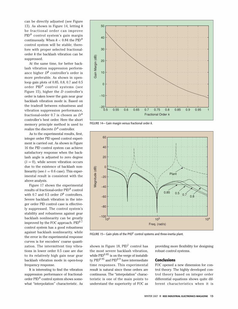
can be directly adjusted (see Figure13). As shown in Figure 14, letting kbe fractional order can improvePIDk control system’s gain margincontinuously. When k < 0.84 the PIDk

control system will be stable; there-fore with proper selected fractional-order k the backlash vibration can besuppressed.

At the same time, for better back-lash vibration suppression perform-ance higher Dk controller’s order ismore preferable. As shown in open-loop gain plots of 0.85, 0.8, 0.7 and 0.5order PIDk control systems (seeFigure 15), higher the D controller’sorder is taken lower the gain near gearbacklash vibration mode is. Based onthe tradeoff between robustness andvibration suppression performance,fractional-order 0.7 is chosen as D k

controller’s best order. Here the shortmemory principle method is used torealize the discrete D k controller.

As to the experimental results, first,integer order PID speed control experi-ment is carried out. As shown in Figure16 the PID control system can achievesatisfactory response when the back-lash angle is adjusted to zero degree(δ = 0), while severe vibration occursdue to the existence of backlash non-linearity (see δ = 0.6 case). This exper-imental result is consistent with theabove analysis.

Figure 17 shows the experimentalresults of fractional-order PIDk controlwith 0.7 and 0.5 order Dk controllers.Severe backlash vibration in the inte-ger order PID control case is effective-ly suppressed. The control system’sstability and robustness against gearbacklash nonlinearity can be greatlyimproved by the FOC approach. PID0.7

control system has a good robustnessagainst backlash nonlinearity, whilethe error in the experimental responsecurves is for encoders’ coarse quanti-zation. The intermittent tiny vibra-tions in lower order 0.5 case are dueto its relatively high gain near gearbacklash vibration mode in open-loopfrequency response.

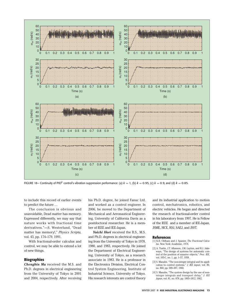
It is interesting to find the vibrationsuppression performance of fractional-order PIDk control system shows some-what “interpolation’’ characteristic. As

shown in Figure 18, PID1 control hasthe most severe backlash vibration,while PID0.85 is on the verge of instabili-ty. PID0.95 and PID0.9 have intermediatetime responses. This experimentalresult is natural since these orders arecontinuous. The “interpolation’’ charac-teristic is one of the main points tounderstand the superiority of FOC as

providing more flexibility for designingrobust control systems.

ConclusionsFOC opened a new dimension for con-trol theory. The highly developed con-trol theory based on integer orderdifferential equations shows quite dif-ferent characteristics when it is

FIGURE 14— Gain margin versus fractional order k.

0.5 0.55 0.6 0.65 0.7 0.75 0.8 0.85 0.9 0.95 1−20

−10

0

10

20

30

40

50

Fractional Order k

Gai

n M

argi

n (d

B)

FIGURE 15— Gain plots of the PIDk control systems and three-inertia plant.

102 103 104−100

−80

−60

−40

−20

0

20

40

60

Freq. (rad/s)

Mag

nitu

de (

dB)

Plant

0.850.70.5

0.8


expanded into a fractional-order field.At the same time, FOC is actually anice generalization of IOC theory. Thisgeneralization gives huge space forresearchers to see conventional IOCtheory in a fresh light and find new andinteresting things.

From a practice viewpoint, the idealfractional-order controllers can only berealized by proper approximation withfinite differential or difference equa-tions. Namely, “design by FOC and real-ize by IOC” are inevitable. Thepractical advantages for FOC is to pro-

vide more flexibility and insight in con-trol design and thus give a clear-cutapproach for designing robust controlsystem. The authors do believe somewell-designed IOC system might in factbe a unconscious approximation ofFOC system.

And the dynamic features of “real”systems can be described more ade-quately by fractional-order models.Especially for light materials and flex-ible structures, not only damping,but also other variety of physicalphenomena such as viscoelasticity

and anomalous relaxation should betaken into account. This demand nat-urally needs fractional-order modelsand hence fractional-order con-trollers, which are hopeful tools formodeling and controlling complexdynamic features.

Finally, the authors would like toend this introduction of FOC with thefollowing expressive quotation:

“… all systems need a fractionaltime derivative in the equations thatdescribe them … systems have memo-ry of all earlier events. It is necessary

FIGURE 16— Time responses of the integer order PID control: (a) δ = 0◦ and (b) δ = 0.6◦ .

0 0.1 0.2 0.3 0.4 0.5 0.6 0.7 0.8 0.9 1 0 0.1 0.2 0.3 0.4 0.5 0.6 0.7 0.8 0.9 1

0 0.1 0.2 0.3 0.4 0.5 0.6 0.7 0.8 0.9 1 0 0.1 0.2 0.3 0.4 0.5 0.6 0.7 0.8 0.9 1

0102030405060

ωm

(ra

d/s

)

05

1015202530

Time (s)

ωl (

rad

/s)

0102030405060

ωm

(ra

d/s

)

05

1015202530

ωl (

rad

/s)

Time (s)

(a) (b)

FIGURE 17— Time responses of PIDk control: (a) k = 0.7 and (b) k = 0.5.

0 0.1 0.2 0.3 0.4 0.5 0.6 0.7 0.8 0.9 10

102030405060

ωm

(ra

d/s

)

05

1015202530

Time (s)

ωl (

rad

/s)

0102030405060

ωm

(ra

d/s

)

05

1015202530

ωl (

rad

/s)

0 0.1 0.2 0.3 0.4 0.5 0.6 0.7 0.8 0.9 1

0 0.1 0.2 0.3 0.4 0.5 0.6 0.7 0.8 0.9 1 0 0.1 0.2 0.3 0.4 0.5 0.6 0.7 0.8 0.9 1

Time (s)

(a) (b)


to include this record of earlier eventsto predict the future …

The conclusion is obvious andunavoidable, Dead matter has memory.Expressed differently, we may say thatnature works with fractional timederivatives.”—S. Westerlund, “Deadmatter has memory!,” Physics Scripta,vol. 43, pp. 174–179, 1991.

With fractional-order calculus andcontrol, we may be able to extend a lotof new things.

BiographiesChengbin Ma received the M.S. andPh.D. degrees in electrical engineeringfrom the University of Tokyo in 2001and 2004, respectively. After receiving

his Ph.D. degree, he joined Fanuc Ltd.and worked as a control engineer. In2006, he moved to the Department ofMechanical and Aeronautical Engineer-ing, University of California Davis as apostdoctoral researcher. He is a mem-ber of IEEE and IEE-Japan.

Yoichi Hori received the B.S., M.S.and Ph.D. degrees in electrical engineer-ing from the University of Tokyo in 1978,1980, and 1983, respectively. He joinedthe Department of Electrical Engineer-ing, University of Tokyo, as a researchassociate in 1983. He is a professor inthe Electronics Division, Electrical Con-trol System Engineering, Institute ofIndustrial Science, University of Tokyo.His research interests are control theory

and its industrial application to motioncontrol, mechatronics, robotics, andelectric vehicles. He began and directedthe research of fractional-order controlin his laboratory from 1997. He is Fellowof the IEEE and a member of IEE-Japan,JSME, SICE, RSJ, SAEJ, and JSST.

References[1] K.B. Oldham and J. Spanier, The Fractional Calcu-

lus. New York: Academic, 1974.

[2] A. Tustin, J.T. Allanson, J.M. Layton, and R.J. Jake-ways, “The design of systems for automatic con-trol of the position of massive objects,” Proc. IEE,vol. 105-C, no. 1, pp. 1–57, 1958.

[3] S. Manabe, “The non-integer integral and its appli-cation to control systems,” J. IEE Japan, vol. 80,no. 860, pp. 589–597, 1960.

[4] S. Manabe, “The system design by the use of non-integer integrals and transport delay,” J. IEEJapan, vol. 81, no. 878, pp. 1803–1812, 1962.

FIGURE 18— Continuity of PIDk control’s vibration suppression performance: (a) k = 1, (b) k = 0.95, (c) k = 0.9, and (d) k = 0.85.

0 0.1 0.2 0.3 0.4 0.5 0.6 0.7 0.8 0.9 10

102030405060

ωm

(ra

d/s)

05

1015202530

Time (s)

ωl (

rad/

s)

0 0.1 0.2 0.3 0.4 0.5 0.6 0.7 0.8 0.9 1

0 0.1 0.2 0.3 0.4 0.5 0.6 0.7 0.8 0.9 1 0 0.1 0.2 0.3 0.4 0.5 0.6 0.7 0.8 0.9 1

Time (s)

(a) (b)

0102030405060

ωm

(ra

d/s)

05

1015202530

ωl (

rad/

s)

0102030405060

ωm

(ra

d/s)

0

0 0.1 0.2 0.3 0.4 0.5 0.6 0.7 0.8 0.9 1

Time (s)

0 0.1 0.2 0.3 0.4 0.5 0.6 0.7 0.8 0.9 1

0 0.1 0.2 0.3 0.4 0.5 0.6 0.7 0.8 0.9 1 0 0.1 0.2 0.3 0.4 0.5 0.6 0.7 0.8 0.9 1

Time (s)

(c) (d)

0

51015202530

ωl (

rad/

s)

0102030405060

ωm

(ra

d/s)

51015202530

ωl (

rad/

s)

BETA

Introducing

Exclusive programming for technology professionals.

Reports from IEEE Spectrum Special Features and more!

FEATURING: Conference Highlights Author Profi les Careers in Technology

access via

IEEE.tv is made possible by the members of IEEE

New programs every month!

Tune in. www.ieee.org/ieeetv

887-Qb IEEEtv 7x4.75.indd 1 8/16/06 11:13:37


[5] S. Manabe, “The system design by the use of amodel consisting of a saturation and non-integer integrals,” J. IEE Japan, vol. 82, no. 890,pp. 1731–1740, 1962.

[6] M. Axtelland and M.E. Bise, “Fractional calculusapplications in control systems,” in Proc. IEEE1990 Nat. Aerospace and Electronics Conf., NewYork, USA, pp. 563–566, 1990.

[7] I. Podlubny, “Fractional differential equations,” inMathematics in Science and Engineering, vol. 198,New York: Academic, 1999.

[8] B.M. Vinagre, V. Feliú, and J.J. Feliú, “Frequencydomain identification of a flexible structure withpiezoelectric actuators using irrational transferfunction,” in Proc. 37th IEEE Conf. Decision andControl, Tampa, FL, pp. 1278–1280, 1998.

[9] L.L. Ludovic, A. Oustaloup, J.C. Trigeassou, and F.Levron, “Frequency identification by non-integermodel,” in Proc. IFAC System Structure and ControlConf., Nantes, France, 1998, pp. 297–302.

[10] J.A. Tenreiro Machado, “Theory analysis anddesign of fractional-order digital control sys-tems,” J. Syst. Anal. Modeling Simulation, vol. 27,no. 2–3, pp. 107–122, 1997.

[11] A. Oustaloup, J. Sabatier, and X. Moreau, “From frac-tal robustness to the CRONE approach,” Euro. SeriesApplied Ind. Math., vol. 5, pp. 177–192, Dec. 1998.

[12] I. Petras, B.M. Vinagre, “Practical application of

digital fractional-order controller to temperaturecontrol,” in Proc. Acta Montanistica Slovaca, vol. 7,no. 2, pp. 131–137, 2002.

[13] W. Li and Y. Hori, “Vibration suppression usingneuron-based pi fuzzy controller and fractional-order disturbance observer,” IEEE Trans. Ind. Elec-tron., vol. 54, no. 1, pp. 117–126, 2007.

[14] I. Petras, B.M. Vinagre, L. Dorcak, and V. Feliú,“Fractional digital control of a heat solid, experi-mental results,” in Proc. 3rd Int. Carpatian ControlConf., Malenovice, Czech Republic, pp. 365–370,2002.

[15] I. Petras, “Control of fractional-order Chua’s sys-tem,” J. Elec. Eng., vol. 53, no. 7–8, pp. 219–222, 2002.

[16] S. Manabe, “A suggestion of fractional-ordercontroller for flexible spacecraft attitude con-trol,” Nonlinear Dynam., vol. 29, no. 1–4, pp.251–268, 2002.

[17] C.W. de Silva, Vibration Fundamentals and Prac-tice. London and New York: CRC, 2000.

[18] A. Oustaloup, F. Levron, and F.M. Nanot, “Fre-quency-band complex noninteger differentiator,characterization and synthesis,” IEEE Trans. Circ.Sys. I, vol. 47, no. 1, pp. 25–39, 2000.

[19] H. Sun, A. Abdelwahab, and B. Onaral, “Linearapproximation of transfer function with a pole offractional power,” IEEE Trans. Automat. Contr.,vol. 29, no. 5, pp. 441–444, 1984.

[20] A. Charef, H. Sun, Y. Tsao, and B. Onaral, “Fractalsystem as represented by singularity function,”IEEE Tran. Automat. Contr., vol. 37, no. 9, pp.1465–1470, 1992.

[21] C. Ma and Y. Hori, “The time-scaled trape-zoidal rule for discrete fractional order con-trol lers,” Nonlinear Dynam. , vol . 38, pp.171–180, 2004.

[22] J.A. Tenreiro Machado, “Discrete-time fractional-order controllers,” Fractional Calculus AppliedAnal., vol. 4, no. 1, pp. 47–66, 2001.

[23] C. Ma, Y. Hori, “Time-domain evaluation of frac-tional order controllers’ direct discretizationmethods,” IEE J. Trans. Ind. Applicat., vol. 124, no.8, pp. 837–842, 2004.

[24] C. Ma, Y. Hori, “Backlash vibration suppressioncontrol of torsional system by novel fractionalorder P ID k controller,” IEE J. Trans. Ind.Applicat., vol. 124, no. 3, pp. 312–317, 2004.

[25] R.S. Barbosa and J.A. Tenreiro Machado,“Describing function analysis of systems withimpacts and backlash,” Nonlinear Dynam., vol.29, no. 1–4, pp. 235–250, 2002.

[26] H. Kobayashi, Y. Nakayama, and K. Fujikawa,“Speed control of multi-inertia system only by aPID controller,” IEE J. Trans. Ind. Applicat., vol.122-D, no. 3, pp. 260–265, 2002.

fractional-order control: theory and applications...

Documents