DOCUMENTOS DE TRABAJO

Calibrating the Dynamic Nelson-Siegel Model: A Practitioner Approach

Francisco Ibáñez

N.º 774 Enero 2016BANCO CENTRAL DE CHILE

BANCO CENTRAL DE CHILE

CENTRAL BANK OF CHILE

La serie Documentos de Trabajo es una publicación del Banco Central de Chile que divulga los trabajos de investigación económica realizados por profesionales de esta institución o encargados por ella a terceros. El objetivo de la serie es aportar al debate temas relevantes y presentar nuevos enfoques en el análisis de los mismos. La difusión de los Documentos de Trabajo sólo intenta facilitar el intercambio de ideas y dar a conocer investigaciones, con carácter preliminar, para su discusión y comentarios.

La publicación de los Documentos de Trabajo no está sujeta a la aprobación previa de los miembros del Consejo del Banco Central de Chile. Tanto el contenido de los Documentos de Trabajo como también los análisis y conclusiones que de ellos se deriven, son de exclusiva responsabilidad de su o sus autores y no reflejan necesariamente la opinión del Banco Central de Chile o de sus Consejeros.

The Working Papers series of the Central Bank of Chile disseminates economic research conducted by Central Bank staff or third parties under the sponsorship of the Bank. The purpose of the series is to contribute to the discussion of relevant issues and develop new analytical or empirical approaches in their analyses. The only aim of the Working Papers is to disseminate preliminary research for its discussion and comments.

Publication of Working Papers is not subject to previous approval by the members of the Board of the Central Bank. The views and conclusions presented in the papers are exclusively those of the author(s) and do not necessarily reflect the position of the Central Bank of Chile or of the Board members.

Documentos de Trabajo del Banco Central de ChileWorking Papers of the Central Bank of Chile

Agustinas 1180, Santiago, ChileTeléfono: (56-2) 3882475; Fax: (56-2) 3882231

Documento de Trabajo

N° 774

Working Paper

N° 774

CALIBRATING THE DYNAMIC NELSON-SIEGEL MODEL:

A PRACTITIONER APPROACH

Francisco Ibáñez

Banco Central de Chile

Abstract

The dynamic version of the Nelson-Siegel model has shown useful applications in the investment

management industry. These applications go from forecasting the yield curve to portfolio risk

management. Because of the complexity in the estimation of the parameters, some practitioners are

unable to benefit from the uses of this model. This note presents two approximations to estimate the

time series of the model’s factors. The first one has a more technical aim, focusing on the

construction of a representative base to work, and uses a genetic algorithm to face the optimization

problem. The second approximation has a practitioner spirit, focusing on the easiness of

implementation. The results show that both methodologies have good fitting for the U.S. Treasury

bonds market.

Resumen

La versión dinámica del modelo Nelson-Siegel ha mostrado útiles aplicaciones para la industria de

gestión de inversiones. Estas extensiones van desde proyectar la curva de rendimientos, hasta la

gestión de riesgo de un portafolio de bonos. Dado que la complejidad en la estimación de los

parámetros es significativa, algunos practicantes no son capaces de beneficiarse de los usos de este

modelo. En esta nota se presentan dos aproximaciones para estimar las series de tiempo de los

factores del modelo. La primera tiene un enfoque más técnico, concentrándose en la construcción de

una base de trabajo representativa, y usa un algoritmo genético para enfrentar el problema de

optimización. La segunda aproximación conserva un espíritu práctico, enfocándose en la facilidad de

su implementación. Los resultados muestran que ambas metodologías poseen un buen ajuste para el

mercado de bonos del Tesoro Estadounidense.

Open Market Trading desk. The author would like to thank Rodolfo J. Prieto, Augusto O. Castillo, Rodrigo A. Alfaro and

Sarah E. Lally for their valuable contributions to this study. Email: fibanez@bcentral.cl.

1 Introduction

Over the last decades, modelling the yield curve has become a major interestfor both academics and investment practitioners. Jones (1991) indicates thatapproximately 95% of the total return of a US Treasury bonds portfolio canbe explained by three type of movements. These movements include parallelshifts (86%), slope twists (9.8%) and butterfly type movements (3.6%). Litter-man and Sheinkman (1991) find similar results and expose the benefits of athree-factor approach (level, slope, curvature) on bond portfolio hedging.

There are many techniques and models to fit a yield curve, but very fewof them end up being as popular as the model proposed by Nelson and Siegel(1987). Diebold and Rudebusch (2013) attribute this success to three main fea-tures. Firstly, the model respects the restrictions imposed by the economic andfinancial theory (e.g. discount factor tends to zero as maturity grows). Sec-ondly, its parsimonious approximation avoids in-sample overfitting, improv-ing its forecasting capacity. Finally, it can take any yield curve form, empiri-cally observed in the market.

Thanks to the great versatility shown by the Nelson-Siegel model and therecent interest of researchers, many extensions of the model have emerged.Some of them include additional variables (Svensson, 1995), and no-arbitrageconditions (Christensen, Diebold and Rudebusch, 2011). Diebold, Ji and Li,(2006) extend the use of the model and show that managing interest rate riskwith a three-factor approach (level, slope and curvature durations), can bemore reliable than a one-factor approach (modified duration and convexity).

Although this model could be a powerful tool in the hands of portfoliomanagers, estimation techniques can result somewhat unfamiliar and techni-cal. This study is organized as follows: the second section introduces, briefly,the Nelson-Siegel model. The third section develops a model calibration for theUS market. The fourth section proposes a practitioner version of the exercise,more pragmatic and replicable. The fifth section concludes.

2 Modelling the yield curve

Nelson and Siegel (1987) modelled the yield curve using three components.The first one remains constant when the term to maturity (τ) varies. The sec-ond factor has more impact on short maturities. The impact of the third factorincreases with maturity, reaches a peak and then decays to zero. The authorsconclude that each one of these three factors governs the part of the yield curvewhere they have more impact; long (β1), short (β2) and medium term (β3), re-spectively. There is a fourth factor (not entirely described), λ, that can be inter-preted as a decay factor. The value of λ affects the fitting power of the modelfor different segments of the curve.

y (τ) = β1 + (β2 + β3)

(1− e−λτ

λτ

)− β3e−λτ (1)

1

Diebold and Li (2006) propose a dynamic version of the model. Firstly, theyreinterpret the three components of the original model as level (lt), slope (st)and curvature (ct), at period t. Secondly, they realise that if the yield curveevolves in time, so do the factors explaining it. This allows the potential use ofthe model for forecasting purposes.

yt (τ) = lt + st

(1− e−λtτ

λtτ

)+ ct

(1− e−λtτ

λtτ− e−λtτ

)(2)

λ introduces a non-linearity in the equation (2). Nelson and Siegel (1987)note that by fixing this parameter, the problem assumes a lineal form, and it canbe solved by OLS. Following this, Diebold and Li (2006) propose the two-stepestimation. The first step of the procedure consists of fixing the decay factor toestimate the parameters. The second step consists of fitting a dynamic model tothe factors

{lt, st, ct

}with a VAR or other relevant model. Diebold and Rude-

busch (2013) analyse various methodologies to estimate the parameters of themodel. The authors note that although more complex methodologies are supe-rior, in principle, they have only slightly better fitting results than the two-stepestimation.

This study has the objective of providing tools to estimate the first partof the two-step methodology. In other words, we intend to fix λ, so we canestimate the time series of level, slope and curvature. We will present twoapproaches. The first one will be a more rigorous approach, from the academicpoint of view. The second one will be more pragmatic, focusing on the easinessof implementation. Both methodologies will focus on the US Treasury market,due to its high liquidity and data availability.

3 Rigorous approach

This approach works on a rich price base, an ideal scenario to calibrate themodel. Though its representation of the bond market is the best and its re-sults are very good, the construction of the price base is time consuming andthe estimation is computationally demanding. The rigorous methodology isdescribed as follows:

• Using a secondary market price base of bills, notes and bonds issued bythe US Treasury, over a determined window, we construct a panel of yieldcurves.

• Bootstrapping the yield curve of each period, we find the spot rates.

• We fit the model on each observation, without fixing the decay factor. Asa result, we get a distribution of λ over the estimation window.

• Finally, we choose the one λ that shows the best fitting power over thewhole window. Then, we can construct the time series for the factors oflevel, slope and curvature.

2

3.1 Data

Choosing the securities to be included in the estimation is no trivial task. Gürkay-nak, Sack and Wright (2007) estimate the parameters of the Nelson-Siegel-Svensson model for the US Treasury yield curve from 1961 to 20061. Althoughthe authors intend to work on a rich sample that, ideally, includes every avail-able security at every observation, they recognise that not all Treasuries arecomparable in terms of liquidity, and specific features (e.g. callable bonds).To address this issue they set a few rules to filter these undesirable securities.Even though our work has a different aim than the cited study (the authors fo-cus on a cross-sectional fit), the treatment of the data under this approach willbe similar.

We set a daily frequency window between December 1999 and December2013. This gives us 3,523 observations. For each period we gather the pricesand features of the securities that had been part of the Barclays U.S. TreasuryIndex and the Barclays U.S. Treasury Bill Index during that day2. The firstincludes notes and bonds issued by the U.S. Government, excluding TIPS andSTRIPS. The second index contains bills with less than a year of maturity. Theless populated observation has 112 bonds and bills, while the most populatedhas 268. On average, we have 166 securities in each yield curve, making thisan almost ideal price base to work with.

For each observation we bootstrap the yield curve, to obtain the spot rates.The roll-down effect and new issuances make it impossible to compare eachcurve directly. To face this problem, Diebold and Li (2006) interpolate the termsto maturity 3, 6, 9, 12, 15, 18, 21, 24, 30, 36, 48, 60, 72, 84, 96, 108 and 120 months.Using cubic splines, we extend their work adding maturities up to 25 years,spaced 12 months from each other. We do not reach the 30 years because thereare some periods when the Treasury stopped issuing 30-year bonds. Addition-ally, and following market practices, we express term to maturity in years. Asa result we obtain a spot rate surface with 32 constant maturities, shown infigure 1.

3.2 Estimation

Our next objective is to find a fixed value of λ that provides the best fit for everyobservation along the window. On each observation we seek to minimize theroot mean squared error (RMSE) between the yields generated by the modeland the spot rates bootstrapped on the previous section. Although this think-ing appears to be straight forward, it is necessary to impose some restrictionson the excercise. By doing this, we can improve the economic interpretation ofthe factors and use less resources solving the optimization problem.

1The resulting yields and the estimated parameters are being constantly updated, and can beaccessed on the website http://www.federalreserve.gov/econresdata/feds/2006/.

2Using both indexes we leave the Treasury notes with maturity less than a year out of thesample. Gürkaynak et al. (2007) argue that short maturity notes often behave oddly, probably dueto the lack of liquidity, and segmented demand.

3

Figure 1: Spot yield surface

2000 2002 2004 2006 2008 2010 2012 2014

0

10

20

30

1

2

3

4

5

6

7

Pe r i odTe r m ( y e ar s )

Spotrate

After bootstrapping each yield curve in the estimation window, we interpolate constant maturitiesfrom 1/4 to 25 years. Each one of these spot rates are comparable over time.

limτ→∞

yt (τ) = lt

While the term to maturity (τ) increases, the equation (2) tends to the levelfactor. According to data published by the United States Treasury, the highestlevel recorded for a 30-year bond is 15.2% (September 1981), and has not ex-ceeded levels over 10% since October 1985. Consistenly with this, we cap lt at15. Negative values for the level factor will imply a negative long term rate,which is inconsistent with the financial theory. For this reason, we set the lowerlimit to zero. By construction, this restriction affects the values that st and ctcan assume. Both can take positive and negative values, so we set their limitsat -15 and 153.

A higher correlation between the slope and curvature factor loadings willaffect the identification of the factors. Gilli, Grobe and Schumann (2010) statethat a lower identification will translate in factors exchanging their values overtime. Figure 2 shows that correlation between the level and slope loadingstends to be perfectly inverse when λt is close to zero. The correlation rapidlyincreases with the decay factor, becoming near perfect for values over 30. Inorder to address the collinearity and identification problem, we will set limitsfor λt between 0 and 30.

3If the instantaneous rate (yt(0)) is zero, the maximum value that the slope (yt(∞)− yt(0)) canassume is the level factor. Analogously, if the instantaneous rate is 15, the slope will be -15, thanksto the restriction of positive long term rate. Similar logic can be applied to set the limit of thecurvature, so they will share the same limits.

4

Figure 2: Correlation between level and slope loadings

5 10 15 20 25 30

−1

0

1

λ

ρ

We graphed the correlation between the level and slope loadings (vertical axis), for each value ofλt. The figure shows that the correlation tends to -1 when the decay factor tends to 0. On the otherhand, the correlation tends to be perfect for λt over 30.

limτ→0

yt (τ) = lt + st

When the term to maturity tends to zero (instantaneous interest rate), theyield provided by equation (2) approximates to the sum of the level and slopefactors. With the objective of having a positive overnight rate, the sum of bothfactors must be positive.

Grouping all restrictions, we are going to resolve the following optimiza-tion problem:

minθ

Z =1√m‖yt − yt‖2 (3)

θ = {lt, st, ct, λt}

s.t.

0 < lt ≤ 15−15 ≤ st ≤ 15−15 ≤ ct ≤ 15

0 < λt ≤ 300 < lt + st

where yt is a vector containing the observed spot yields at period t, whileyt is a vector that contains yields provided by the equation (2), for each of them terms of the curve.

Gilli et al. (2010) identify three major problems with estimating this model.Firstly, the optimization problem is nonconvex, showing multiple local optima.Secondly, the model is badly-conditioned for a certain range of parameters,thus the estimates are unstable before small price movements. Finally, thevalue of the decay factor directly affects the correlation between the loadings of

5

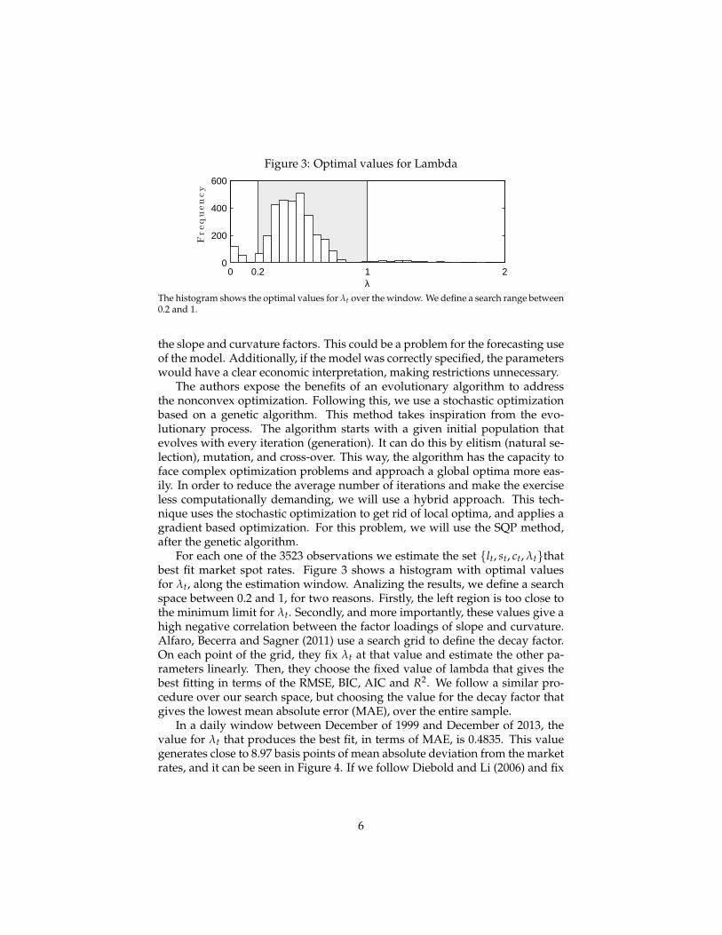
Figure 3: Optimal values for Lambda

0 0.2 1 20

200

400

600

λ

Frequency

The histogram shows the optimal values for λt over the window. We define a search range between0.2 and 1.

the slope and curvature factors. This could be a problem for the forecasting useof the model. Additionally, if the model was correctly specified, the parameterswould have a clear economic interpretation, making restrictions unnecessary.

The authors expose the benefits of an evolutionary algorithm to addressthe nonconvex optimization. Following this, we use a stochastic optimizationbased on a genetic algorithm. This method takes inspiration from the evo-lutionary process. The algorithm starts with a given initial population thatevolves with every iteration (generation). It can do this by elitism (natural se-lection), mutation, and cross-over. This way, the algorithm has the capacity toface complex optimization problems and approach a global optima more eas-ily. In order to reduce the average number of iterations and make the exerciseless computationally demanding, we will use a hybrid approach. This tech-nique uses the stochastic optimization to get rid of local optima, and applies agradient based optimization. For this problem, we will use the SQP method,after the genetic algorithm.

For each one of the 3523 observations we estimate the set {lt, st, ct, λt}thatbest fit market spot rates. Figure 3 shows a histogram with optimal valuesfor λt, along the estimation window. Analizing the results, we define a searchspace between 0.2 and 1, for two reasons. Firstly, the left region is too close tothe minimum limit for λt. Secondly, and more importantly, these values give ahigh negative correlation between the factor loadings of slope and curvature.Alfaro, Becerra and Sagner (2011) use a search grid to define the decay factor.On each point of the grid, they fix λt at that value and estimate the other pa-rameters linearly. Then, they choose the fixed value of lambda that gives thebest fitting in terms of the RMSE, BIC, AIC and R2. We follow a similar pro-cedure over our search space, but choosing the value for the decay factor thatgives the lowest mean absolute error (MAE), over the entire sample.

In a daily window between December of 1999 and December of 2013, thevalue for λt that produces the best fit, in terms of MAE, is 0.4835. This valuegenerates close to 8.97 basis points of mean absolute deviation from the marketrates, and it can be seen in Figure 4. If we follow Diebold and Li (2006) and fix

6

Figure 4: Mean absolute error

0.2 0.3 0.4 0.5 0.6 0.7 0.8 0.9 1

10

15

20

λ

MAE

(bp)

the value of the decay factor at 0.73084, we get 12.12 basis points of error. Werecognize two possible reasons for this. Firstly, the authors do not perform anoptimization excercise to find this value. Instead, they fix λt at the value thatmaximizes the loading on the curvature factor at exactly 30 months. Secondly,their excercise considers maturities up to 10 years. Because we fit the model onrates up to 25 years, there could be a loss of fit on the longer maturities. Becausethe methodology proposed on this study is able to deliver better results thanusing the decay factor of the original work, we are content with it.

4 Practitioner Approach

Although the methodology described in the previous section shows a stronggoodness of fit, the amount of time required to construct the base to work withis high, and the optimization procedure can become computationally demand-ing. Now we present a more pragmatical methodology that can be replicatedby investment analysts. The practitioner methodology is described as follows:

• Using public and free data, we construct a spot rates surface.

• Then, we find a fixed value for λ, without a resource consuming calibra-tion. This way, the methodology remains as simple as possible.

• Finally, we estimate the time series for the factors of level, slope and cur-vature. We use the restricted least squares (RLS) method, so we can in-corporate restrictions imposed in the previous section.

4.1 Data

We use the information provided by the United States Treasury, and the FederalReserve of Saint Luis Economic Data (FRED). On a daily basis, they publishyields to maturities for Government securities with 1/12, 1/4, 1/2, 1, 2, 3, 5, 7,10, 20 and 30 years to maturity. These are commonly referred to as Constant

4The authors propose 0.0609. Because they measure term to maturity in terms of months, weannualize their value.

7

Maturity Treasury rates (CMT)5, and are a result of an interpolation on theclosing market bid yields of actively traded securities. We define an estimationwindow with the same features specified in the previous section. Using thetime series of the CMT we bootstrap every observation. Using cubic splines,we interpolate the same terms defined in the other approach, then we constructthe spot yield surface. As a result, we have a rates base completely comparablewith the one generated in the previous section.

4.2 Estimation

Diebold and Li (2006) noted that λt determines the maturity where the factorloading reaches its highest value. They fixed the decay factor at 0.0609, placingthe maximum loading at 30 months, which is consistent with the empirical ev-idence about the curvature. The main advantage of this analysis is that it doesnot depend on the base you work on. This makes the model easily adaptableto other economies and windows.

Gilli et al (2010) find that for a certain range of values for λt the factor load-ings of slope and curvature become highly correlated. This problem couldtranslate in collinearity within the model, allowing parameters to exchangewith each other at their estimation. If we fit a cross-section model, collinearityis not a problem itself6. It becomes an issue when using the model with fore-casting purpose, because of the need for stable and identifiable time series offactors.

minλ

R = ρ2FS ,FC

(4)

FS =

(1− e−λτ1

)(λτ1)

−1(1− e−λτ2

)(λτ2)

−1

...(1− e−λτn

)(λτn)

−1

, FC =

(1− e−λτ1

)(λτ1)

−1 − e−λτ1(1− e−λτ2

)(λτ2)

−1 − e−λτ2

...(1− e−λτn

)(λτn)

−1 − e−λτn

We intend to fix λt using a similiar logic described in the previous para-

graph. Instead of focusing on the curvature maximization, we try to work onthe correlation problem, exposed by Gilli et al. (2010). In the excercise (4) welook for the λ that minimizes the squared correlation between the slope (FS)and curvature (FC) factor loadings. To evaluate the correlation, we create avector τ containing daily terms to maturity between 30 days up to 30 years.After running the optimization, the decay factor that nullifies the correlation is0.2262. In order to linearize the estimation of the model, and face its collinearityproblem, we fix λt at this value7.

5These securities assume a semiannual payment. In case of maturities below a year, the Trea-sury uses recently issued bills and estimates their bond equivalent yield.

6Actually, fitting the model without fixing the decay factor will increase its degrees of freedom.7It is not necessary for the practitioner to repeat this process. This value can be used to linearize

the model for any 30-year yield curve, of any economy.

8

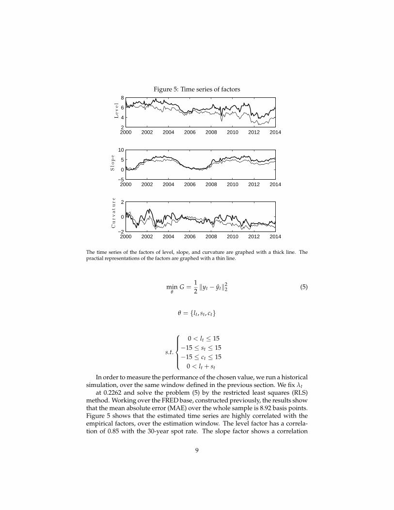
Figure 5: Time series of factors

2000 2002 2004 2006 2008 2010 2012 20142

4

6

8

Level

2000 2002 2004 2006 2008 2010 2012 2014−5

0

5

10

Slo

pe

2000 2002 2004 2006 2008 2010 2012 2014−2

0

2

Curvature

The time series of the factors of level, slope, and curvature are graphed with a thick line. Thepractial representations of the factors are graphed with a thin line.

minθ

G =12‖yt − yt‖2

2 (5)

θ = {lt, st, ct}

s.t.

0 < lt ≤ 15

−15 ≤ st ≤ 15−15 ≤ ct ≤ 15

0 < lt + st

In order to measure the performance of the chosen value, we run a historicalsimulation, over the same window defined in the previous section. We fix λt

at 0.2262 and solve the problem (5) by the restricted least squares (RLS)method. Working over the FRED base, constructed previously, the results showthat the mean absolute error (MAE) over the whole sample is 8.92 basis points.Figure 5 shows that the estimated time series are highly correlated with theempirical factors, over the estimation window. The level factor has a correla-tion of 0.85 with the 30-year spot rate. The slope factor shows a correlation

9

of 0.97 with the negative of the slope (measured with the difference betweenthe 3-month and the 30-year spot rates). The curvature factor has a correlationof 0.55 with a butterfly constructed with the 3-month, 2-year and 30-year spotrates. Using the value proposed by Diebold and Li (2006), we obtain a MAEof 12.47 basis points. Our results are satisfactory because by using the decayfactor proposed in this section, we are able to achieve a better fit, in contrastto using the value suggested by the original study. Additionally we are able toface the collinearity problem.

5 Conclusions

Modelling the yield curve has never been a trivial process. This is the principalreason it is still one of the most prominent focuses of fixed income researchover the decades. Few models have shown the success and popularity of theNelson-Siegel model. This could be attributed to its parsimonious and intuitiveinterpretations of its factors (level, slope, and curvature).

The extension that transforms it in a dynamic model has allowed other usesto be discovered. The most known application is the ability to forecast thefactors, and hence, the entire yield curve.

This note has described two methodologies to estimate the time series ofthe factors. The first uses a very rich Treasury securities price base and fitsthe model using a hybrid optimization method with a genetic algorithm toface the optimization problem. The second methodology presented has a morepractitioner approach. It works on a publicly available base, and linearizes theproblem fixing the decay factor at the value that minimizes the correlation be-tween the slope and curvature factor loadings. Over an estimation window,with daily frequency, between December of 1999 and December of 2013, bothapproaches provide a good fit, in terms of mean absolute error (MAE). Therigourous approach gives an average deviation of 8.97 basis points, from mar-ket rates. The practitioner approach deviates 8.92 basis points, on average. Asa reference point, we estimated the deviaton for both methodologies, fixing λat the value proposed by Diebold and Li (2006). Our results are satisfactorybecause both methodologies proposed to fix the decay factor show better fit, incomparison with the original study.

References

[1] Alfaro, R., Becerra, S., and Sagner, A. Estimación de la estructura de tasasnominales en Chile: Aplicación del modelo dinámico de Nelson-Siegel.Economía Chilena, 14(3):57–74, 2011.

[2] Christensen, J. H. E., Diebold, F. X., and Rudebusch, G. D. The affinearbitrage-free class of Nelson-Siegel term structure models. Journal ofEconometrics, (164):4–20, 2011.

10

[3] Diebold, F. X., Ji, L., and Li, C. A three-factor yield curve model: Non-affine structure, systematic risk sources and generalized duration. Macroe-conomics, Finance and Econometrics: Essay in Memory of Albert Ando, pages240–274, 2006.

[4] Diebold, F. X. and Li, C. Forecasting the term structure of governmentbond yields. Journal of Econometrics, 130:337–364, 2006.

[5] Diebold, F. X. and Rudebusch, G. D. Yield Curve Modeling and Forecasting:The Dynamic Nelson-Siegel Approach. Princeton University Press, 2013.

[6] Gilli, M., Grosse, S., and Schumann, E. Calibrating the Nelson-Siegel-Svensson model. COMISEF Working Paper Series No.31, 2010.

[7] Gürkaynak, R. S., Sack, B., and Wright, J. H. The U.S. Treasury yieldcurve: 1961 to the present. Journal of Monetary Economics, 54(8):2291–2304,November 2007.

[8] Jones, F. J. Yield curve strategies. The Journal of Fixed Income, 1(2):43–48,1991.

[9] Litterman, R. and Scheinkman, J. Common factors affecting bond returns.The Journal of Fixed Income, 1(1):54–61, 1991.

[10] Nelson, C. R. and Siegel, A. F. Parsimonious modeling of yield curves.Journal of Business, 60(4):473–489, 1987.

[11] Svensson, L. Estimating forward interest rates with the extended Nelson-Siegel method. Sveriges Riskbank Quarterly Review, 3:13–26, 1995.

11

A Matlab Code

%% P a r a m e t e r s .c lear , c l cs e r i e s = { ’DGS3MO’ ’DGS6MO’ ’DGS1 ’ ’DGS2 ’ ’DGS3 ’ ’DGS5 ’ ’DGS7 ’ . . .

’DGS10 ’ ’DGS20 ’ ’DGS30 ’ } ;cmt_terms = [3/12 6/12 1 2 3 5 7 10 20 3 0 ] ;spot_terms = [3/12 6/12 9/12 12/12 15/12 18/12 21/12 24/12 3 0 / 1 2 . . .

36/12 4 : 1 : 3 0 ] ;window ={ ’ 12/31/1999 ’ ’ 12/31/2013 ’ } ;t o l = 3 ; % T o l e r a n c e f o r m i s s i n g d a t a from FRED .lambda = 0 . 2 2 6 2 ;

%% CMT y i e l d s b a s e c o n s t r u c t i o n .% C o n e c t i o n with FRED .conect ion = fred ( ’ h t tps :// research . s t l o u i s f e d . org/fred2/ ’ ) ;n s e r i e s = length ( s e r i e s ) ; % We count t h e number o f s e r i e s .for i = 1 : n s e r i e s

get = f e t c h ( conect ion , s e r i e s ( i ) , window ( 1 ) , window ( 2 ) ) ;i f i == 1

cmt_dates = get . Data ( : , 1 ) ;cmt_ytm = zeros ( length ( get . Data ) , n s e r i e s ) ;

endcmt_ytm ( : , i ) = get . Data ( : , 2 ) ;

endclose ( conect ion )c l e a r i get n s e r i e s conect ion s e r i e s window

% We c l e a n t h e b a s e o f m i s s i n g d a t a o b s e r v a t i o n s .index = sum( isnan ( cmt_ytm ) , 2 ) > t o l ;count = 0 ;for i = 1 : length ( cmt_dates )

i f index ( i ) == 1cmt_ytm ( i − count , : ) = [ ] ;cmt_dates ( i − count , : ) = [ ] ;count = count + 1 ;

endendc l e a r i count index t o l

%% B o o t s t r a p p i n g t h e y i e l d s u r f a c e .spot_sur f = zeros ( length ( cmt_dates ) , length ( spot_terms ) ) ;for i = 1 : length ( cmt_dates )

aux = [ cmt_ytm ( i , : ) ’ / 1 0 0 zeros ( length ( cmt_terms ) , 1 ) ] ;for j = 1 : length ( cmt_terms )

aux ( j , 2 ) = addtodate ( cmt_dates ( i , 1 ) , . . .cmt_terms ( j )∗1 2 , ’month ’ ) ;

endaux = aux (~any ( isnan ( aux ) , 2 ) , : ) ;[ z , t ] = pyld2zero ( aux ( : , 1 ) , aux ( : , 2 ) , cmt_dates ( i ) ) ;t = y e a r f r a c ( cmt_dates ( i ) , t ) ;spot_sur f ( i , : ) = spline ( t , z , spot_terms )∗1 0 0 ;

endclc , c l e a r i j z t aux

%% Curve F i t t i n g .loadings = zeros ( length ( spot_terms ) , 3 ) ;

12

loadings ( : , 1 ) = 1 ;loadings ( : , 2 ) = (1−exp(−lambda .∗ spot_terms ’ ) ) . / . . .

( lambda .∗ spot_terms ’ ) ;loadings ( : , 3 ) = (1−exp(−lambda .∗ spot_terms ’ ) ) . / . . .

( lambda .∗ spot_terms ’)−exp(−lambda .∗ spot_terms ’ ) ;l s c = zeros ( length ( cmt_dates ) , 3 ) ; % Time s e r i e s v e c t o r .

% O p t i m i z a t i o n .bounds = [0 −15 −15; 15 15 1 5 ] ; % P a r a m e t e r s b o u n d r i e s .r e s t = [−1 ,−1 ,0]; % ( b1 + b2 ) > 0opt = optimoptions ( @lsql in , ’ Display ’ , ’ o f f ’ , ’ Algorithm ’ , ’ ac t ive−s e t ’ ) ;for i = 1 : length ( cmt_dates )

l s c ( i , : ) = l s q l i n ( loadings , spot_sur f ( i , : ) , r e s t , 0 , [ ] , [ ] , . . .bounds ( 1 , : ) , bounds ( 2 , : ) , [ ] , opt ) ;

end

13

Documentos de Trabajo

Banco Central de Chile

NÚMEROS ANTERIORES

La serie de Documentos de Trabajo en versión PDF

puede obtenerse gratis en la dirección electrónica:

www.bcentral.cl/esp/estpub/estudios/dtbc.

Existe la posibilidad de solicitar una copia impresa

con un costo de Ch$500 si es dentro de Chile y

US$12 si es fuera de Chile. Las solicitudes se pueden

hacer por fax: +56 2 26702231 o a través del correo

electrónico: bcch@bcentral.cl.

Working Papers

Central Bank of Chile

PAST ISSUES

Working Papers in PDF format can be

downloaded free of charge from:

www.bcentral.cl/eng/stdpub/studies/workingpaper.

Printed versions can be ordered individually for

US$12 per copy (for order inside Chile the charge

is Ch$500.) Orders can be placed by fax: +56 2

26702231 or by email: bcch@bcentral.cl.

DTBC – 773

Terms of Trade Shocks and Investment in Commodity-Exporting Economies

Jorge Fornero, Markus Kirchner y Andrés Yany

DTBC – 772

Explaining the Cyclical Volatility of Consumer Debt Risk

Carlos Madeira

DTBC – 771

Channels of US Monetary Policy Spillovers into International Bond Markets

Elías Albagli, Luis Ceballos, Sebastián Claro y Damián Romero

DTBC – 770

Fuelling Future Prices: Oil Price and Global Inflation

Carlos Medel

DTBC – 769

Inflation Dynamics and the Hybrid Neo Keynesian Phillips Curve: The Case of Chile

Carlos Medel

DTBC – 768

The Out-of-sample Performance of an Exact Median-unbiased Estimator for the

Near-unity AR(1) Model

Carlos Medel y Pablo Pincheira

DTBC – 767

Decomposing Long-term Interest Rates: An International Comparison

Luis Ceballos y Damián Romero

DTBC – 766

Análisis de Riesgo de los Deudores Hipotecarios en Chile

Andrés Alegría y Jorge Bravo

DTBC – 765

Economic Performance, Wealth Distribution and Credit Restrictions Under Variable

Investment: The Open Economy

Ronald Fischer y Diego Huerta

DTBC – 764

Country Shocks, Monetary Policy Expectations and ECB Decisions. A Dynamic Non-

Linear Approach

Máximo Camacho, Danilo Leiva-León y Gabriel Péres-Quiros

DTBC – 763

Dynamics of Global Business Cycles Interdependence

Lorenzo Ductor y Danilo Leiva-León

DTBC – 762

Bank’s Price Setting and Lending Maturity: Evidence from an Inflation Targeting

Economy

Emiliano Luttini y Michael Perdersen

DTBC – 761

The Resource Curse: Does Fiscal Policy Make a Difference?

Álvaro Aguirre y Mario Giarda

DTBC – 760

A Microstructure Approach to Gross Portfolio Inflows: The Case of Chile

Bárbara Ulloa, Carlos Saavedra y Carola Moreno

DTBC – 759

Efectos Reales de Cambios en el Precio de la Energía Eléctrica

Lucas Bertinato, Javier García-Cicco, Santiago Justel y Diego Saravia

DOCUMENTOS DE TRABAJO • Enero 2016