from kandel, schwartz and jessel, principles of neural...

4 Concept neurons — Introduction to artificial neural networks4.1 Typical neuron/nerve cell:

from Kandel, Schwartz and Jessel, Principles of Neural Science

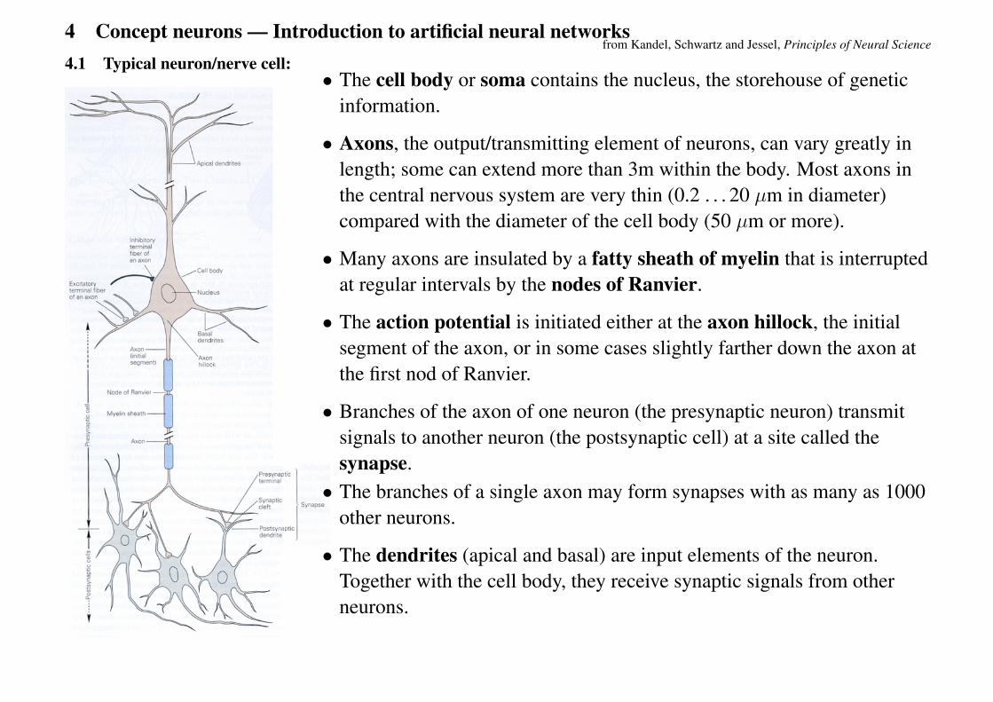
• The cell body or soma contains the nucleus, the storehouse of geneticinformation.

• Axons, the output/transmitting element of neurons, can vary greatly inlength; some can extend more than 3m within the body. Most axons inthe central nervous system are very thin (0.2 . . . 20 µm in diameter)compared with the diameter of the cell body (50 µm or more).

• Many axons are insulated by a fatty sheath of myelin that is interruptedat regular intervals by the nodes of Ranvier.

• The action potential is initiated either at the axon hillock, the initialsegment of the axon, or in some cases slightly farther down the axon atthe first nod of Ranvier.

• Branches of the axon of one neuron (the presynaptic neuron) transmitsignals to another neuron (the postsynaptic cell) at a site called thesynapse.

• The branches of a single axon may form synapses with as many as 1000other neurons.

• The dendrites (apical and basal) are input elements of the neuron.Together with the cell body, they receive synaptic signals from otherneurons.

Intro. Comp. NeuroSci. — Ch. 4 August 10, 2005

Simplified functions of these very complex in their nature “building blocks” of a neuron are as follow:

• The synapses are elementary signal processing devices.

– A synapse is a biochemical device which converts a pre-synaptic electrical signal into a chemicalsignal and then back into a post-synaptic electrical signal.

– The input pulse train has its amplitude modified by parameters stored in the synapse. The nature ofthis modification depends on the type of the synapse, which can be either inhibitory or excitatory.

• The postsynaptic signals are aggregated and transferred along the dendrites to the nerve cell body.

• The cell body generates the output neuronal signal, activation potential, which is transferred along theaxon to the synaptic terminals of other neurons.

• The frequency of firing of a neuron is proportional to the total synaptic activities and is controlled bythe synaptic parameters (weights).

• The pyramidal cell can receive 104 synaptic inputs and it can fan-out the output signal to thousands oftarget cells — the connectivity difficult to achieve in the artificial neural networks.

Other examples of neurons can be found in:http://www.csse.monash.edu.au/courseware/cse2330/Lnts/neurons/

A.P. Paplinski 4–2


4.2 A simplistic model of a biological neuron

t

xi

t

Dendrite

Axon

Synapses

Post−synaptic signal

Axon−HillockCell Body (Soma)

Activation potential

Output Signal, j

x

y

Input Signals,

y j

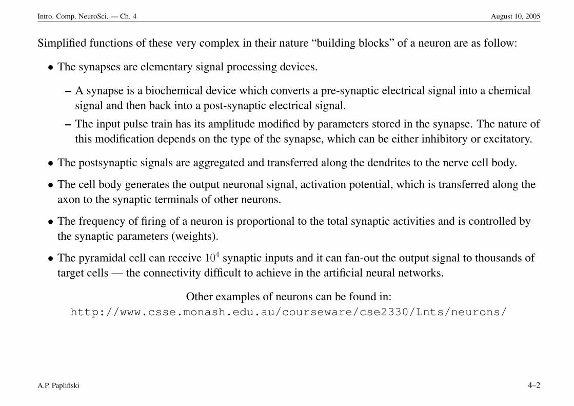
Figure 4–1: Conceptual structure of a biological neuron

Basic characteristics of a biological neuron:

• data is coded in a form of instantaneous frequency of pulses

• synapses are either excitatory or inhibitory

• Signals are aggregated (“summed”) when travel along dendritic trees

• The cell body (neuron output) generates the output pulse train of an average frequency proportional tothe total (aggregated) post-synaptic activity (activation potential).



4.3 Models of artificial neurons

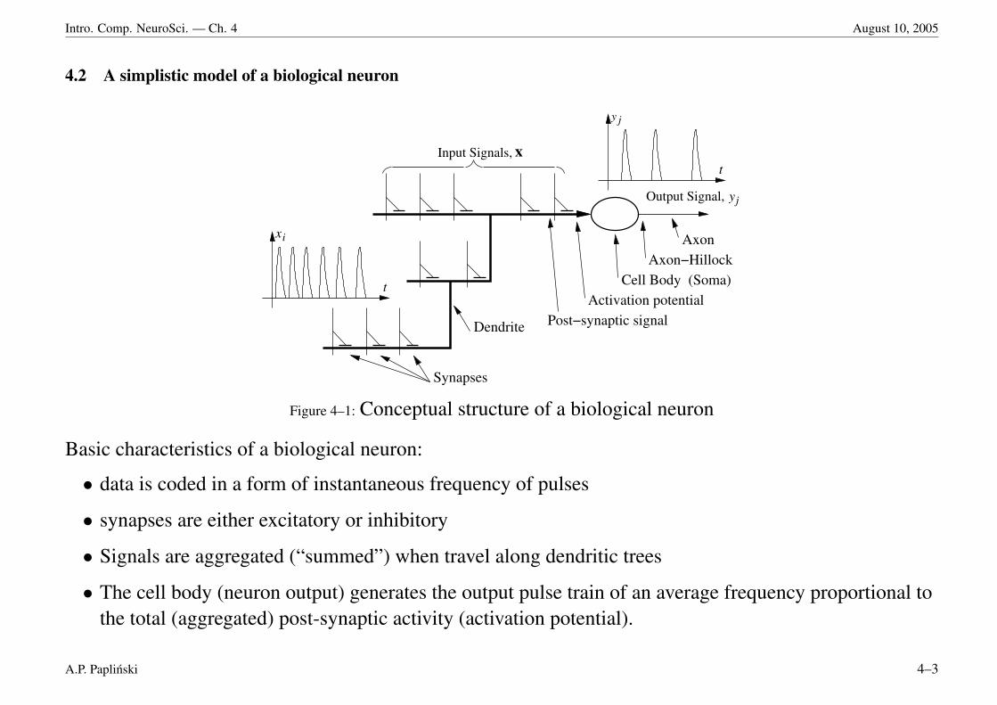
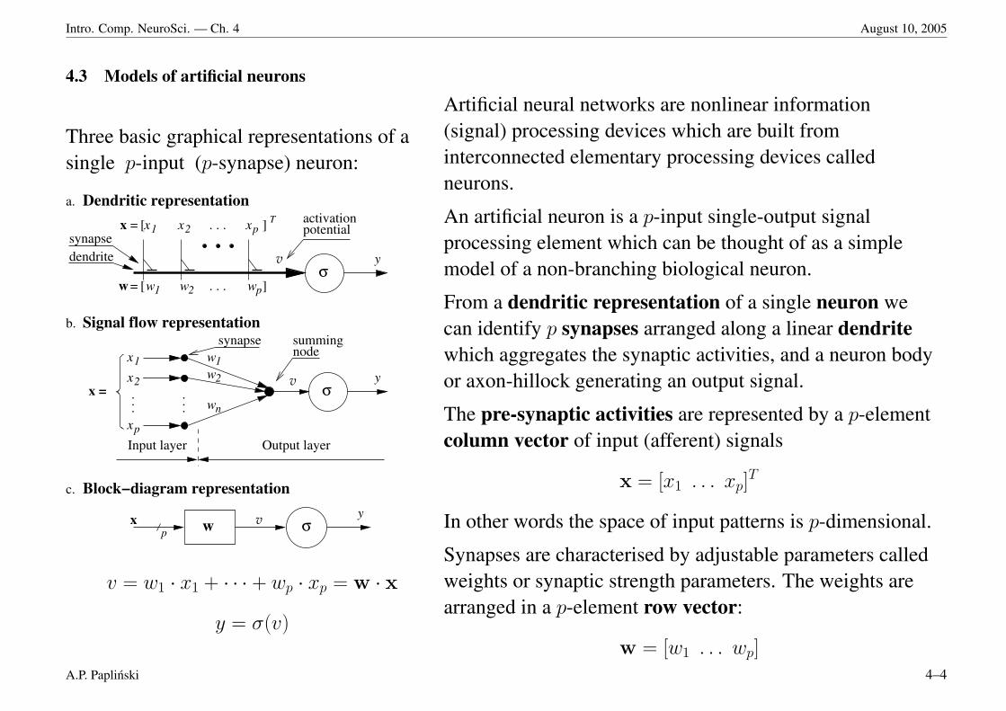
Three basic graphical representations of asingle p-input (p-synapse) neuron:

.

. ...

summingnode

. . .

. . .

x1

y

w1

= [

= [ ]

] Tx

w

xx2

w2 w

p

p

vsynapsedendrite

a.activationpotential

Input layer Output layerx

x2

x1

y

w1

y

x =

x w

p

p

v

v

synapse

c.

Dendritic representation

b.

Block−diagram representation

σ

σ

σ

w

Signal flow representation

2

wn.

v = w1 · x1 + · · · + wp · xp = w · x

y = σ(v)

Artificial neural networks are nonlinear information(signal) processing devices which are built frominterconnected elementary processing devices calledneurons.

An artificial neuron is a p-input single-output signalprocessing element which can be thought of as a simplemodel of a non-branching biological neuron.

From a dendritic representation of a single neuron wecan identify p synapses arranged along a linear dendritewhich aggregates the synaptic activities, and a neuron bodyor axon-hillock generating an output signal.

The pre-synaptic activities are represented by a p-elementcolumn vector of input (afferent) signals

x = [x1 . . . xp]T

In other words the space of input patterns is p-dimensional.

Synapses are characterised by adjustable parameters calledweights or synaptic strength parameters. The weights arearranged in a p-element row vector:

w = [w1 . . . wp]A.P. Paplinski 4–4


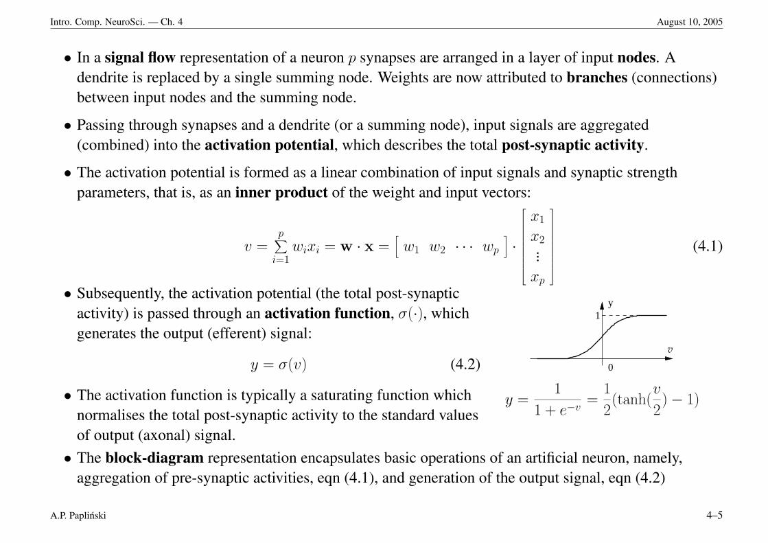
• In a signal flow representation of a neuron p synapses are arranged in a layer of input nodes. Adendrite is replaced by a single summing node. Weights are now attributed to branches (connections)between input nodes and the summing node.

• Passing through synapses and a dendrite (or a summing node), input signals are aggregated(combined) into the activation potential, which describes the total post-synaptic activity.

• The activation potential is formed as a linear combination of input signals and synaptic strengthparameters, that is, as an inner product of the weight and input vectors:

v =p∑

i=1wixi = w · x =

[w1 w2 · · · wp

]·

x1

x2...

xp

(4.1)

• Subsequently, the activation potential (the total post-synapticactivity) is passed through an activation function, σ(·), whichgenerates the output (efferent) signal:

y = σ(v) (4.2)

• The activation function is typically a saturating function whichnormalises the total post-synaptic activity to the standard valuesof output (axonal) signal.

y1

0

v

y =1

1 + e−v=

1

2(tanh(

v

2)− 1)

• The block-diagram representation encapsulates basic operations of an artificial neuron, namely,aggregation of pre-synaptic activities, eqn (4.1), and generation of the output signal, eqn (4.2)



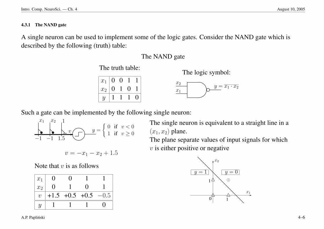
4.3.1 The NAND gate

A single neuron can be used to implement some of the logic gates. Consider the NAND gate which isdescribed by the following (truth) table:

The NAND gate

The truth table:

x1 0 0 1 1x2 0 1 0 1y 1 1 1 0

The logic symbol:x2

x1

$%g y = x1 · x2

Such a gate can be implemented by the following single neuron:

v

y =

0 if v < 01 if v ≥ 0@ @u u @

x1 x2 1

−1 −1 1.5-

v = −x1 − x2 + 1.5

Note that v is as follows

x1 0 0 1 1x2 0 1 0 1v +1.5 +0.5 +0.5 −0.5

y 1 1 1 0

The single neuron is equivalent to a straight line in a(x1, x2) plane.The plane separate values of input signals for whichv is either positive or negative

-x1

6x2

0 1

1

4 4

4 y = 1 y = 0

@@

@@

@@

@@

@@

@@



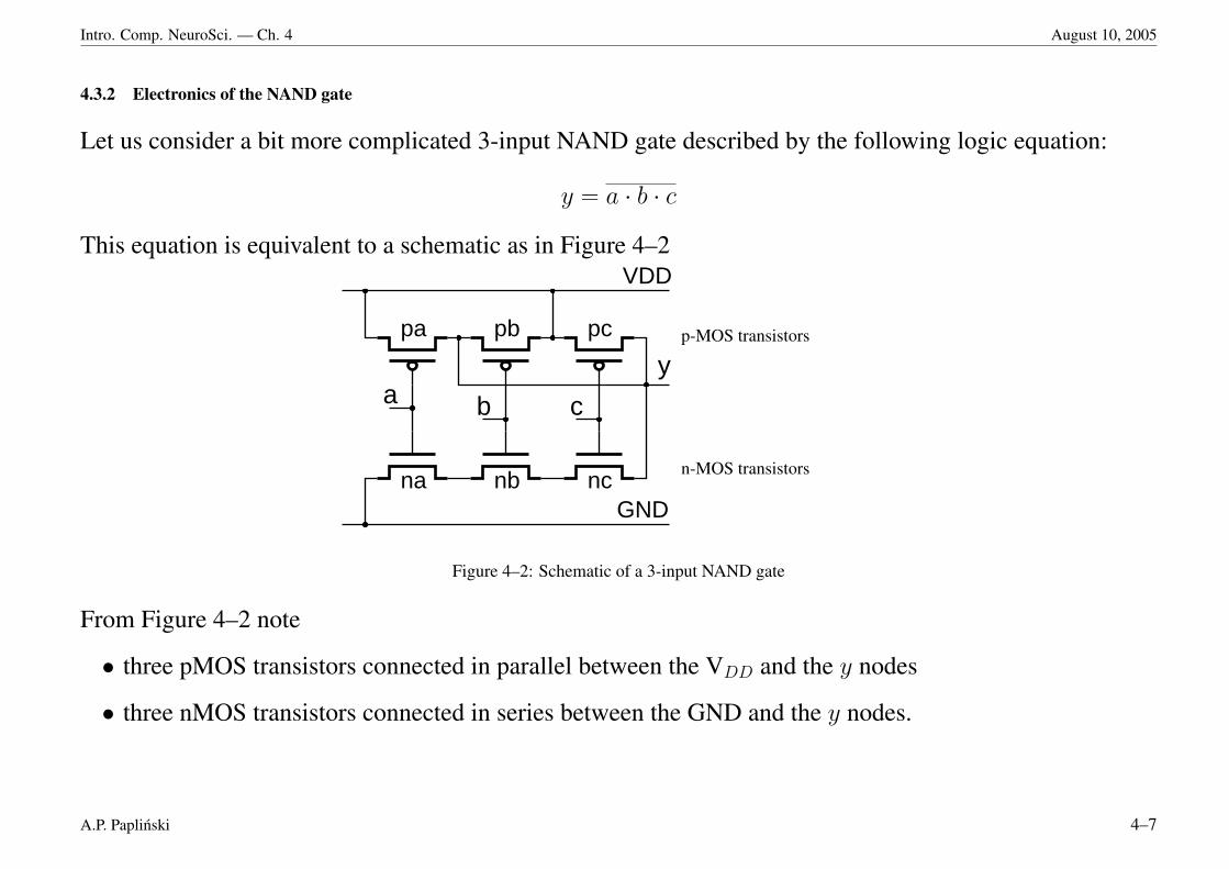
4.3.2 Electronics of the NAND gate

Let us consider a bit more complicated 3-input NAND gate described by the following logic equation:

y = a · b · c

This equation is equivalent to a schematic as in Figure 4–2

pa pb

na nb

y a b

GND

VDD

pc

nc

c

p-MOS transistors

n-MOS transistors

Figure 4–2: Schematic of a 3-input NAND gate

From Figure 4–2 note

• three pMOS transistors connected in parallel between the VDD and the y nodes

• three nMOS transistors connected in series between the GND and the y nodes.



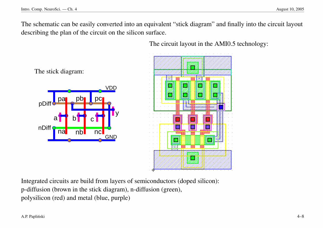
The schematic can be easily converted into an equivalent “stick diagram” and finally into the circuit layoutdescribing the plan of the circuit on the silicon surface.

The stick diagram:

y a b

pa pb

na nb

VDD

GND

nDiff

pDiffpc

nc

c

The circuit layout in the AMI0.5 technology:

Integrated circuits are build from layers of semiconductors (doped silicon):p-diffusion (brown in the stick diagram), n-diffusion (green),polysilicon (red) and metal (blue, purple)



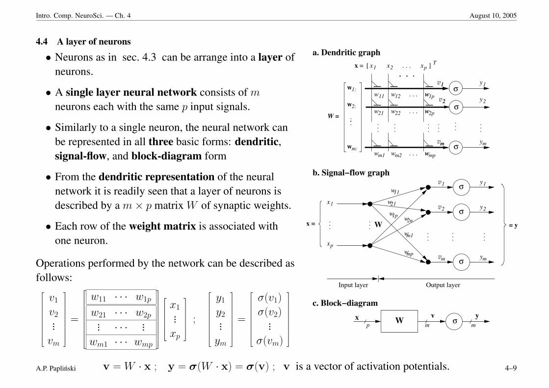
4.4 A layer of neurons

• Neurons as in sec. 4.3 can be arrange into a layer ofneurons.

• A single layer neural network consists of m

neurons each with the same p input signals.

• Similarly to a single neuron, the neural network canbe represented in all three basic forms: dendritic,signal-flow, and block-diagram form

• From the dendritic representation of the neuralnetwork it is readily seen that a layer of neurons isdescribed by a m× p matrix W of synaptic weights.

• Each row of the weight matrix is associated withone neuron.

Operations performed by the network can be described asfollows:

v1

v2...

vm

=

w11 · · · w1p

w21 · · · w2p... · · · ...

wm1 · · · wmp

x1...

xp

;

y1

y2...

ym

=

σ(v1)

σ(v2)...

σ(vm)

......

......

......

. . .

. . .

. . .

w

w

ww

w

w11

21

2n

m1

2

m y

y2

m

W

Input layer Output layer

= yx =

xp

1p

mp

1v

v

v

x ]

w w w

yw w w

y1

w w

y

2

m

w

= [ 1

11

21

m1

12

m2

2

m

1

x

w

w

w

2

m

1

x2 x

..

1:

2:

m:

w

w

w

.

1p

v

v

v

2p

mp

pT

W = ...

. . .

22

b. Signal−flow graph

c. Block−diagram

σ

σ

σ

σ

σ

σ

a. Dendritic graph

px

m

vσ

m

y

x

W

1

... ...... ...

1y

...

v = W · x ; y = σ(W · x) = σ(v) ; v is a vector of activation potentials.A.P. Paplinski 4–9


• From the signal-flow graph it is visible that each weight parameter wij (synaptic strength) is nowrelated to a connection between nodes of the input layer and the output layer.

• Therefore, the name connection strengths for the weights is also justifiable.

• The block-diagram representation of the single layer neural network is the most compact one, henceoften most convenient to use.

• A layer of neurons can be connected together to form a multi-layer structure.

• Multi-layer feedforward networks are known also as Multilayer Perceptrons (MLPs).



4.5 Static and Dynamic Systems — General Concepts

Static systems — feedforward networks

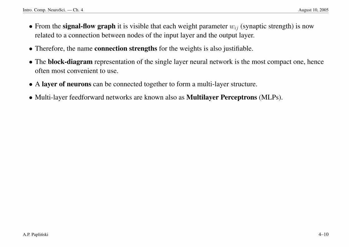
Neural networks considered in previous sections belong to the class of static systems which can be fullydescribed by a set of m-functions of p-variables as in Figure 4–3.

f(x)-x

op

-y

om

Figure 4–3: A static system: y = f (x)

The defining feature of the static systems is that they are time-independent — current outputs dependsonly on the current inputs in the way specified by the mapping function, f .Such a function can be very complex.

Dynamic systems — Recurrent Neural Networks

In the dynamic systems, the current output signals depend, in general, on current and past input signals.

There are two equivalent classes of dynamic systems: continuous-time and discrete-time systems.

The dynamic neural networks are referred to as recurrent neural networks.



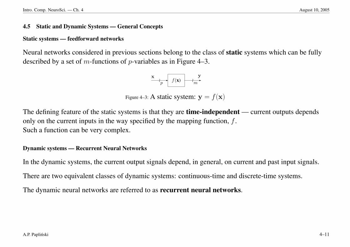
4.6 Continuous-time dynamic systems

• Continuous-time dynamic systems operate with signals which are functions of a continuous variable,t, interpreted typically as time. A spatial variable can be also used.

• Continuous-time dynamic systems are described by means of differential equations. The mostconvenient yet general description uses only first-order differential equations in the following form:

y(t) = f (x(t),y(t)) (4.3)

wherey(t) df=

dy(t)

dtis a vector of time derivatives of output signals.

• In order to model a dynamic system, or to obtain the output signals, the integration operation isrequired. The dynamic system of eqn (4.3) is illustrated in Figure 4–4.

f(x,y)-

xop

-om

-yom

∫-y

om

s

Figure 4–4: A continuous-time dynamic system: y(t) = f(x(t),y(t))

• It is evident that feedback is inherent to dynamic systems.



4.6.1 Discrete-time dynamic systems

• Discrete-time dynamic systems operate with signals which are functions of a discrete variable, n,interpreted typically as time, but a discrete spatial variable can be also used.

• Typically, the discrete variable can be thought of as a sampled version of a continuous variable:

t = n · ts ; t ∈ R , n ∈ N

and ts is the sampling time

• Analogously, discrete-time dynamic systems are described by means of difference equations.

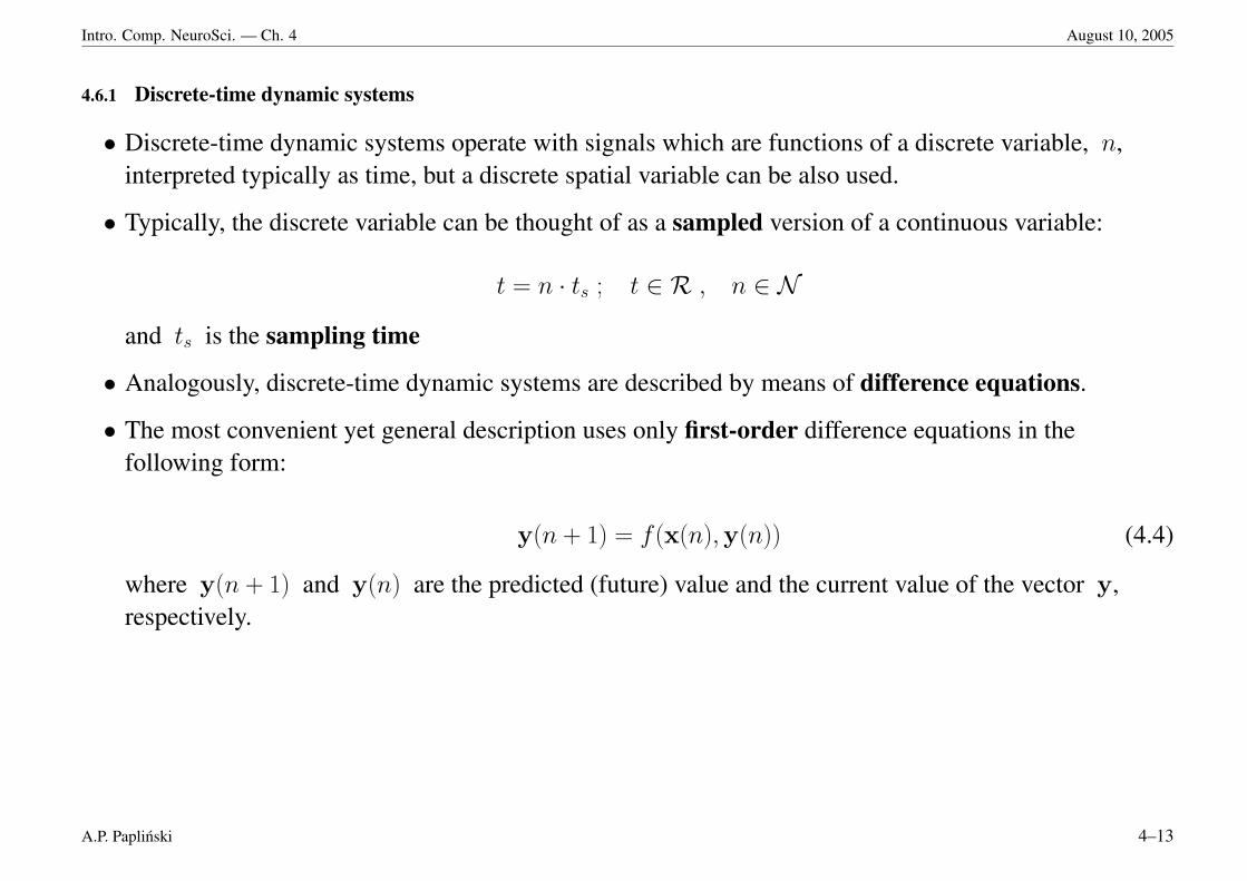
• The most convenient yet general description uses only first-order difference equations in thefollowing form:

y(n + 1) = f (x(n),y(n)) (4.4)

where y(n + 1) and y(n) are the predicted (future) value and the current value of the vector y,respectively.



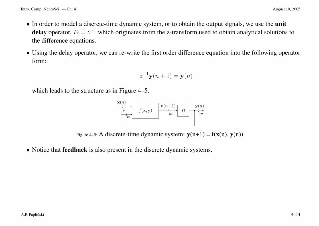
• In order to model a discrete-time dynamic system, or to obtain the output signals, we use the unitdelay operator, D = z−1 which originates from the z-transform used to obtain analytical solutions tothe difference equations.

• Using the delay operator, we can re-write the first order difference equation into the following operatorform:

z−1y(n + 1) = y(n)

which leads to the structure as in Figure 4–5.

f(x,y)-

x(n)op

-om

-y(n+1)

om

D -y(n)om

s

Figure 4–5: A discrete-time dynamic system: y(n+1) = f(x(n), y(n))

• Notice that feedback is also present in the discrete dynamic systems.



4.6.2 Example: A continuous-time generator of a sinusoid

• As a simple example of a continuous-time dynamic system let us consider a linear system whichgenerates a sinusoidal signal.

• Eqn (4.3) takes on the following form: y(t) = A · y(t) + B · x(t) (4.5)

where y =

y1

y2

; A =

0 ω

−ω 0

; B =

0

b

; x = δ(t)

δ(t) is the unit impulse which is non-zero only for t = 0 and is used to describe the initial condition.

• In order to show that eqn (4.5) really describes the sinusoidal generator we re-write this equation forindividual components. This yields:

y1 = ω y2 (4.6)y2 = −ω y1 + b δ(t)

• Differentiation of the first equation and substitution of the second one gives the second-order lineardifferential equation for the output signal y1:

y1 + ω2y1 = ω b δ(t)

• Taking the Laplace transform and remembering that Lδ(t) = 1, we have:

y1(s) = bω

s2 + ω2



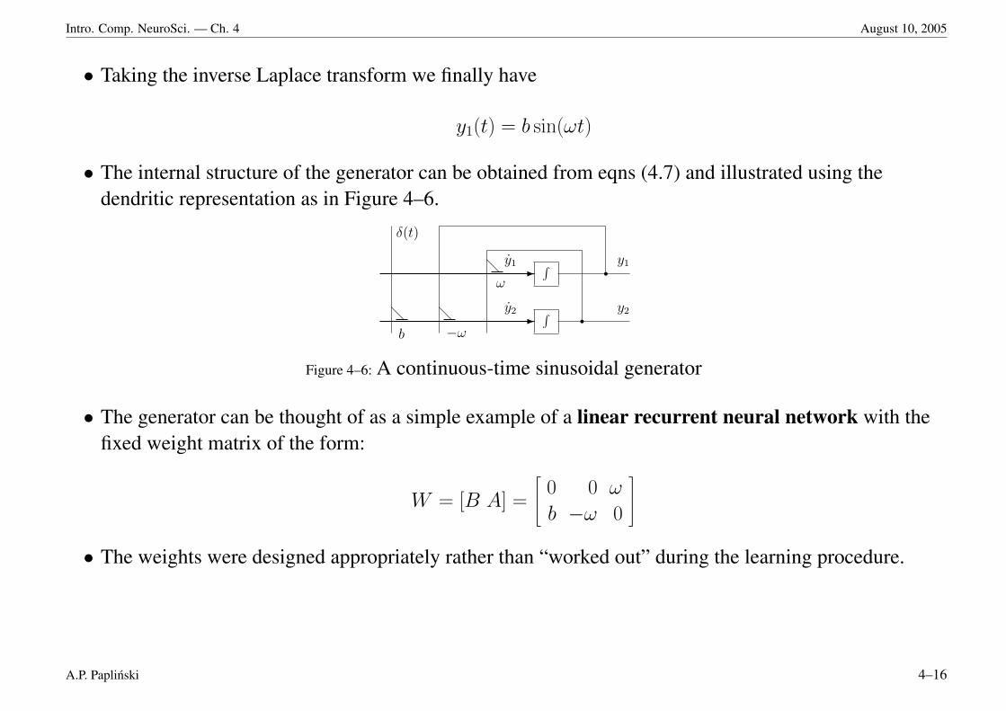
• Taking the inverse Laplace transform we finally have

y1(t) = b sin(ωt)

• The internal structure of the generator can be obtained from eqns (4.7) and illustrated using thedendritic representation as in Figure 4–6.

-

-

∫y1 y1

∫y2 y2

δ(t)

@

b

r@

−ωr

@

ω

Figure 4–6: A continuous-time sinusoidal generator

• The generator can be thought of as a simple example of a linear recurrent neural network with thefixed weight matrix of the form:

W = [B A] =

0 0 ω

b −ω 0

• The weights were designed appropriately rather than “worked out” during the learning procedure.



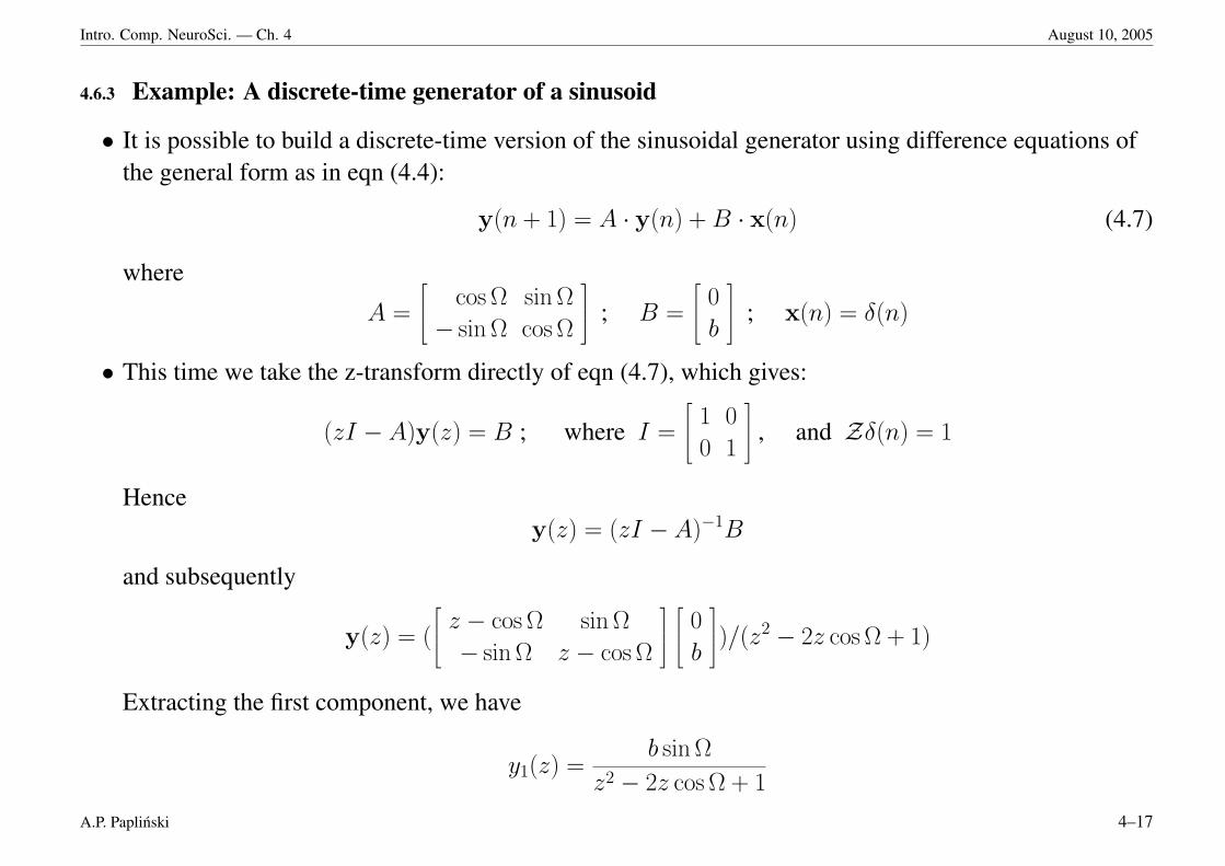
4.6.3 Example: A discrete-time generator of a sinusoid

• It is possible to build a discrete-time version of the sinusoidal generator using difference equations ofthe general form as in eqn (4.4):

y(n + 1) = A · y(n) + B · x(n) (4.7)

where

A =

cos Ω sin Ω

− sin Ω cos Ω

; B =

0

b

; x(n) = δ(n)

• This time we take the z-transform directly of eqn (4.7), which gives:

(zI − A)y(z) = B ; where I =

1 0

0 1

, and Zδ(n) = 1

Hencey(z) = (zI − A)−1B

and subsequently

y(z) = (

z − cos Ω sin Ω

− sin Ω z − cos Ω

0

b

)/(z2 − 2z cos Ω + 1)

Extracting the first component, we have

y1(z) =b sin Ω

z2 − 2z cos Ω + 1



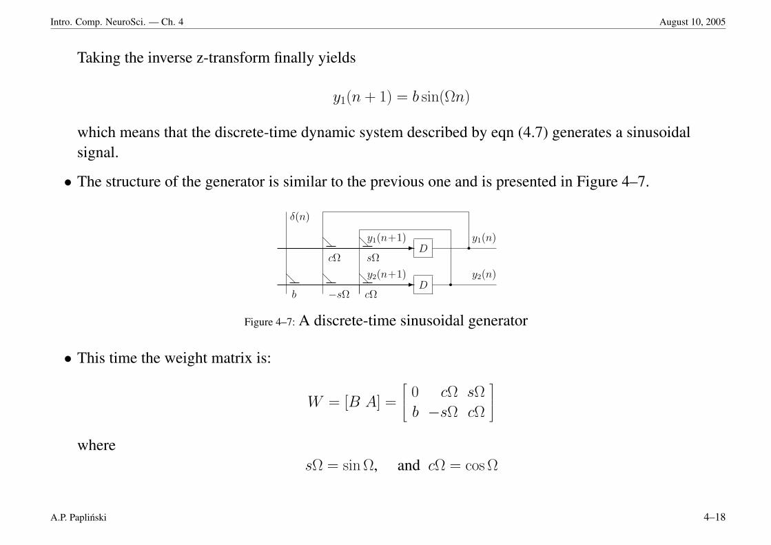
Taking the inverse z-transform finally yields

y1(n + 1) = b sin(Ωn)

which means that the discrete-time dynamic system described by eqn (4.7) generates a sinusoidalsignal.

• The structure of the generator is similar to the previous one and is presented in Figure 4–7.

-

-

Dy1(n+1) y1(n)

Dy2(n+1) y2(n)

δ(n)

@

b

r@

cΩ

@

−sΩr

@

sΩ

@

cΩ

Figure 4–7: A discrete-time sinusoidal generator

• This time the weight matrix is:

W = [B A] =

0 cΩ sΩ

b −sΩ cΩ

wheresΩ = sin Ω, and cΩ = cos Ω



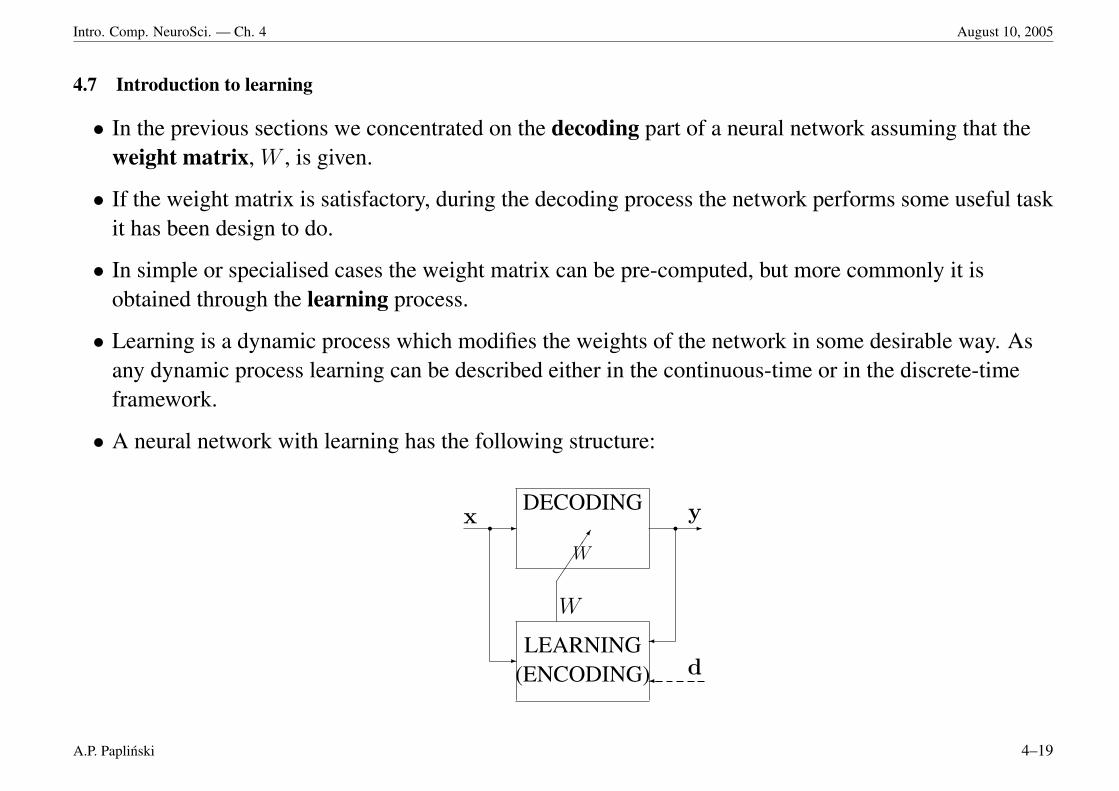
4.7 Introduction to learning

• In the previous sections we concentrated on the decoding part of a neural network assuming that theweight matrix, W , is given.

• If the weight matrix is satisfactory, during the decoding process the network performs some useful taskit has been design to do.

• In simple or specialised cases the weight matrix can be pre-computed, but more commonly it isobtained through the learning process.

• Learning is a dynamic process which modifies the weights of the network in some desirable way. Asany dynamic process learning can be described either in the continuous-time or in the discrete-timeframework.

• A neural network with learning has the following structure:

DECODING

W

LEARNING(ENCODING)

W

-x r

-

-yr

d



• The learning can be described either by differential equations (continuous-time)

W (t) = L( W (t),x(t),y(t),d(t) ) (4.8)

or by the difference equations (discrete-time)

W (n + 1) = L( W (n),x(n),y(n),d(n) ) (4.9)

where d is an external teaching/supervising signal used in supervised learning.

• This signal in not present in networks employing unsupervised learning.

• The discrete-time learning law is often used in a form of a weight update equation:

W (n + 1) = W (n) + ∆W (n) (4.10)∆W (n) = L( W (n),x(n),y(n),d(n) )


from kandel, schwartz and jessel, principles of neural...

Documents