function approximation using back...

i

FUNCTION APPROXIMATION USING BACK PROPAGATION ALGORITHM IN

ARTIFICIAL NEURAL NETWORKS

A THESIS SUBMITTED IN PARTIAL FULFILLMENT OF THE

REQUIREMENTS FOR THE DEGREE OF

Bachelor of Technology

In

Electrical Engineering

By

VANKADARA NVD MANOHAR GAURAV UDAY CHAUDHARI

BISWAJIT MOHANTY

Department of Electrical Engineering

National Institute of Technology

Rourkela

2007

ii

FUNCTION APPROXIMATION USING BACK PROPAGATION ALGORITHM IN


A THESIS SUBMITTED IN PARTIAL FULFILLMENT OF THE

REQUIREMENTS FOR THE DEGREE OF

Bachelor of Technology

In

Electrical Engineering

By

VANKADARA NVD MANOHAR GAURAV UDAY CHAUDHARI

BISWAJIT MOHANTY

Under the Guidance of

Mrs. K.R. SUBHASHINI

Department of Electrical Engineering


Rourkela

2007

iii


Rourkela

CERTIFICATE This is to certify that the thesis entitled, “FUNCTION APPROXIMATION USING BACK

PROPAGATION ALGORITHM IN ARTIFICIAL NEURAL NETWORKS” submitted

by Mr. Gaurav Uday Chaudhari, Mr. V. Manohar, Mr. Biswajit Mohanty in partial fulfillment

of the requirements of the award of Bachelor of Technology Degree in Electrical Engineering

at the National Institute of Technology, Rourkela (Deemed University) is an authentic work

carried out by them under my supervision and guidance.

To the best of my knowledge, the matter embodied in the thesis has not been submitted to any

other university / institute for the award of any Degree or Diploma.

Date: Mrs. K. R. SUBHASHINI

(Lecturer) Dept. of Electrical Engg.

National Institute of Technology Rourkela - 769008

iv

A C K N O W L E D G E M E N T

I wish to express my profound sense of deepest gratitude to my guide and motivator

Mrs. K. R. Subhashini, Lecturer, Electrical Engineering Department, National Institute of

Technology, Rourkela for her valuable guidance, sympathy and co-operation and finally help

for providing necessary facilities and sources during the entire period of this project.

I wish to convey my sincere gratitude to all the faculties of Electrical Engineering

Department who have enlightened me during my studies. The facilities and co-operation

received from the technical staff of Electrical Engg. Dept. are thankfully acknowledged.

I express my thanks to all those who helped me in one way or other.

Last, but not least, I would like to thank the authors of various research articles and

book that referred to.

Biswajit Mohanty Roll No: 10302023 National Institute of

Technology, Rourkela

Gaurav Uday Chaudhari Roll No: 10302012 National Institute of


V. Manohar Roll No: 10302024 National Institute of


v

C O N T E N T S

1 ADAPTIVE SYSTEMS 1

1.1 INTRODUCTION 2

1.2 LINEAR & NON LINEAR MODELS 4

2 ARTIFICIAL NEURAL NETWORKS 5

2.1 INTRODUCTION 6

2.2 WHY ANN? 6

2.3 HISTORICAL OVERVIEW 8

2.4 BIOLOGICAL NEURAL NETWORKS 8

2.5 ARTIFICIAL NEURAL NETWORKS 10

3 STRUCTURE OF ANN 11

3.1 NETWORK ARCHITECTURE 12

3.2 MULTILAYER PERCEPTRONS 13

3.3 STRUCTURE OF A NEURON 14

4 BACK PROPAGATION ALGORITHM 15

4.1 LEARNING 16

4.2 BPA ALGORITHM 17

4.3 BPA FLOWCHART 18

4.4 DATA FLOW DESIGN 19

vi

5 CHALLENGING PROBLEMS 21

5.1 PATTERN RECOGNITION 22

5.2 CLUSTERING 22

5.3 PREDICTION/FORECASTING 22

5.4 OPTIMIZATION 22

5.5 CONTENT ADDRESSABLE MEMORY 23

5.6 FUNCTION APPROXIMATION

6 CHANNEL EQUALIZATION 24

6.1 INTRODUCTION 25

6.2 NEED FOR EQUALIZATION 25

6.3 CLASSIFICATION OF EQUALIZER 27

6.4 NEURAL NETWORK EQUALIZER 27

7 FIXED STRUCTURE ANN 29

7.1 STRUCTURE 30

7.2 RESULTS 31

8 GENERALIZED STRUCTURE ANN 36

8.1 STRUCTURE 37

8.2 RESULTS 38

9 CONCLUSION & DISCUSSION 59

vii

A B S T R A C T

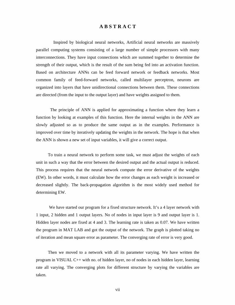
Inspired by biological neural networks, Artificial neural networks are massively

parallel computing systems consisting of a large number of simple processors with many

interconnections. They have input connections which are summed together to determine the

strength of their output, which is the result of the sum being fed into an activation function.

Based on architecture ANNs can be feed forward network or feedback networks. Most

common family of feed-forward networks, called multilayer perceptron, neurons are

organized into layers that have unidirectional connections between them. These connections

are directed (from the input to the output layer) and have weights assigned to them.

The principle of ANN is applied for approximating a function where they learn a

function by looking at examples of this function. Here the internal weights in the ANN are

slowly adjusted so as to produce the same output as in the examples. Performance is

improved over time by iteratively updating the weights in the network. The hope is that when

the ANN is shown a new set of input variables, it will give a correct output.

To train a neural network to perform some task, we must adjust the weights of each

unit in such a way that the error between the desired output and the actual output is reduced.

This process requires that the neural network compute the error derivative of the weights

(EW). In other words, it must calculate how the error changes as each weight is increased or

decreased slightly. The back-propagation algorithm is the most widely used method for

determining EW.

We have started our program for a fixed structure network. It’s a 4 layer network with

1 input, 2 hidden and 1 output layers. No of nodes in input layer is 9 and output layer is 1.

Hidden layer nodes are fixed at 4 and 3. The learning rate is taken as 0.07. We have written

the program in MAT LAB and got the output of the network. The graph is plotted taking no

of iteration and mean square error as parameter. The converging rate of error is very good.

Then we moved to a network with all its parameter varying. We have written the

program in VISUAL C++ with no. of hidden layer, no of nodes in each hidden layer, learning

rate all varying. The converging plots for different structure by varying the variables are

taken.

1

Chapter 1

ADAPTIVE SYSTEMS INTRODUCTION

LINEAR& NONLINEAR MODELS

2

INTRODUCTION

ADAPTIVE SYSTEMS

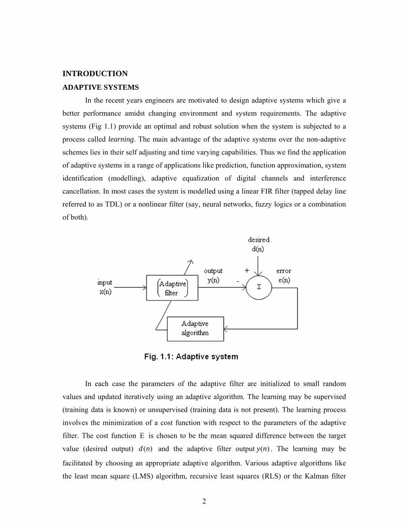
In the recent years engineers are motivated to design adaptive systems which give a

better performance amidst changing environment and system requirements. The adaptive

systems (Fig 1.1) provide an optimal and robust solution when the system is subjected to a

process called learning. The main advantage of the adaptive systems over the non-adaptive

schemes lies in their self adjusting and time varying capabilities. Thus we find the application

of adaptive systems in a range of applications like prediction, function approximation, system

identification (modelling), adaptive equalization of digital channels and interference

cancellation. In most cases the system is modelled using a linear FIR filter (tapped delay line

referred to as TDL) or a nonlinear filter (say, neural networks, fuzzy logics or a combination

of both).

In each case the parameters of the adaptive filter are initialized to small random

values and updated iteratively using an adaptive algorithm. The learning may be supervised

(training data is known) or unsupervised (training data is not present). The learning process

involves the minimization of a cost function with respect to the parameters of the adaptive

filter. The cost function Ε is chosen to be the mean squared difference between the target

value (desired output) )(nd and the adaptive filter output )(ny . The learning may be

facilitated by choosing an appropriate adaptive algorithm. Various adaptive algorithms like

the least mean square (LMS) algorithm, recursive least squares (RLS) or the Kalman filter

3

algorithm may be applied for learning. For instance the LMS algorithm provides robust

performance by iteratively minimizing the mean square error in the direction opposite to the

gradient of the cost function with respect to the parameters )(nwi of a TDL filter (see

Fig.1.2). This can be expressed as

∑=

=P

nneE

1

2 )( (1.1)

where the error over P ensembles of a training data set is given by )()()( nyndne −= (1.2) If the output of the adaptive filter is given as ∑ −=

ii inxnwny )(*)()( (1.3)

then the parameters )(nwi are updated using a learning rate η as

)(

*)()1(nw

Enwnwi

ii ∂∂

−=+ η (1.4)

LINEAR FILTER:

+

e(n)

d(n)

wN-1

y(n)

w2 w1 w0

x(n) Z-

1 Z-1 Z-1

∑

Fig 1.2: Tapped Delay Line Filter

- ∑

4

LINEAR& NON-LINEAR MODELS

The models may be classified as linear or nonlinear depending on the architecture.

Linear systems are modelled on the tapped delay line filter. They are the simplest structures

that can be realized. They require least computational complexity and training period. But

such systems can never approach the optimal performance since they can at the best provide a

linear classification of the received data. This may be compensated by increasing the filter

length and employing a nonlinear cost function as the criterion. In most cases it has been

observed that an increase in the filter length (or order) enhances the additive white Gaussian

noise.

This leads to the definition of an optimal performance since nonlinear process

involving the construction of a nonlinear decision boundary between the received data points

(channel states) belonging to the various classes of data symbols used in transmission. Thus

an optimal model operates with the least number of misclassifications. Due to the above said

drawbacks of the linear models we used here the nonlinear models (ARTIFICIAL NEURAL

NETWORKS, ANN) for our function approximation problem.

5

Chapter 2


INTRODUCTION

WHY ANN?

HISTORICAL OVERVIEW

BIOLOGICAL NEURAL NETWORKS


6

INTRODUCTION


Numerous advances have been made in developing intelligent systems, some inspired

by biological neural networks. Researchers from many scientific disciplines are designing

artificial neural networks (ANN) to solve a variety of problems in pattern recognition,

function approximation, prediction, optimization, associative memory, and control.

Conventional approaches have been proposed for solving these problems. Although

successful applications can be found in certain well-constrained environments, none is

flexible enough to perform well outside its domain. ANNs provide exciting alternatives, and

many applications could benefit from using them.

We discuss the motivations behind the development of ANNs , describe the basic biological

neuron and the artificial computational model, outline network architectures and learning

processes, and present some of the most commonly used ANN models. We conclude with

function approximation a successful ANN application.

WHY ARTIFICIAL NEURAL NETWORKS?

The long course of evolution has given the human brain many desirable characteristics that

are not present in Von Neumann system or in modern parallel computers. These include

massive parallelism,

distributed representation and computation,

learning ability,

generalization ability,

adaptivity,

inherent contextual information processing,

fault tolerance, and

low energy consumption.

It is hoped that devices based on biological neural networks will possess some of these

desirable characteristics.

7

Modern digital computers outperform humans in the domain of numeric computation

and related symbol manipulation. However, humans can effortlessly solve complex

perceptual problems (like recognizing a man in a crowd from a mere glimpse of his face) at

such a high speed and extent as to dwarf the world’s fastest computer. Why is there such a

remarkable difference in their performance? The biological neural system architecture is

completely different from the von Neumann architecture. This difference significantly affects

the type of functions each computational model can best perform.

Numerous efforts to develop “intelligent” programs based on von Neumann’s

centralized architecture have not resulted in general-purpose intelligent programs. Inspired by

biological neural networks, ANNs are massively parallel computing systems consisting of an

extremely large number of simple processors with many interconnections. ANN models

attempt to use some “organizational” principles believed to be used in the human brain.

Modelling a biological nervous system using ANNs can also increase our

understanding of biological functions. State-of-the-art computer hardware technology (such

as VLSI and optical) has made this modelling feasible.

A thorough study of ANNs requires knowledge of neurophysiology, cognitive

science/psychology, physics (statistical mechanics), control theory, computer science,

artificial intelligence, statistics/mathematics, pattern recognition, computer vision, parallel

processing, and hardware (digital/analog/VLSI/optical). New developments in these

disciplines continuously nourish the field. On the other hand, ANNs also provide an impetus

to these disciplines in the form of new tools and representations. This symbiosis is necessary

for the vitality of neural network research. Communications among these disciplines ought to

be encouraged.

8

HISTORICAL OVERVIEW

ANN research has experienced three periods of extensive activity. The first peak in

the 1940s was due to McCulloch and Pitts' pioneering work. The second occurred in the

1960s with Rosenblatt's perceptron convergence theorem and Minsky and Papert's work

showing the limitations of a simple perceptron. Minsky and Papert's results dampened the

enthusiasm of most researchers, especially those in the computer science community. The

resulting lull in neural network research lasted almost 20 years. Since the early 1980s, ANNs

have received considerable renewed interest. The major developments behind this resurgence

include Hopfield's energy approach in 1982 and the back-propagation learning algorithm for

multilayer perceptrons (multilayer feed forward networks) first proposed by Werbos,

reinvented several times, and then popularized by Rumelhart et aL in 1986. Anderson and

Rosenfeld provide a detailed historical account of ANN developments.

BIOLOGICAL NUERAL NETWORKS

A neuron (or nerve cell) is a special biological cell that processes information. It is

composed of a cell body, and two types of out-reaching tree-like branches: the axon and the

dendrites. The cell body has a nucleus that contains information about hereditary traits and

plasma that holds the molecular equipment for producing material needed by the neuron. A

neuron receives signals (impulses) from other neurons through its dendrites (receivers) and

transmits signals generated by its cell body along the axon (transmitter), which eventually

branches into strands and sub strands. At the terminals of these strands are the synapses. A

synapse is an elementary structure and functional unit between two neurons (an axon strand

of one neuron and a dendrite of another), When the impulse reaches the synapse's terminal,

certain chemicals called neurotransmitters are released. The neurotransmitters diffuse across

the synaptic gap, to enhance or inhibit, depending on the type of the synapse, the receptor

neuron's own tendency to emit electrical impulses. The synapse's effectiveness can be

adjusted by the signals passing through it so that the synapses can learn from the activities in

which they participate. This dependence on history acts as a memory, which is possibly

responsible for human memory.

9

Fig 2.1: A SKETCH OF BIOLOGICAL NEURON

The cerebral cortex in humans is a large flat sheet of neurons about 2 to 3 millimeters

thick with a surface area of about 2,200 cm2, about twice the area of a standard computer

keyboard. The cerebral cortex contains about 1011 neurons, which is approximately the

number of stars in the Milky Way. Neurons are massively connected, much more complex

and dense than telephone networks. Each neuron is connected to 103 to 104 other neurons. In

total, the human brain contains approximately 1014 to 1015 interconnections.

Neurons communicate through a very short train of pulses, typically milliseconds in

duration. The message is modulated on the pulse-transmission frequency. This frequency can

vary from a few to several hundred hertz, which is a million times slower than the fastest

switching speed in electronic circuits. However, complex perceptual decisions such as face

recognition are typically made by humans within a few hundred milliseconds. These

decisions are made by a network of neurons whose operational speed is only a few

milliseconds. This implies that the computations cannot take more than about 100 serial

stages. In other words, the brain runs parallel programs that are about 100 steps long for such

perceptual tasks. This is known as the hundred step rule. The same timing considerations

show that the amount of information sent from one neuron to another must be very small (a

few bits). This implies that critical information is not transmitted directly, but captured and

distributed in the interconnections-hence the name, connectionist model, used to describe

ANNs.

10


Artificial neurons are similar to their biological counterparts. They have input

connections which are summed together to determine the strength of their output, which is

the result of the sum being fed into an activation function. Though many activation functions

exist, the most common is the sigmoid activation function, which outputs a number between

0 (for low input values) and 1 (for high input values). The resultant of this function is then

passed as the input to other neurons through more connections, each of which are weighted.

These weights determine the behaviour of the network.

In the human brain the neurons are connected in a seemingly random order and send

impulses asynchronously. If we wanted to model a brain this might be the way to organize an

ANN, but since we primarily want to create a function approximator, ANNs are usually not

organized like this.

When we create ANNs, the neurons are usually ordered in layers with connections

going between the layers. The first layer contains the input neurons and the last layer contains

the output neurons. These input and output neurons represent the input and output variables

of the function that we want to approximate. Between the input and the output layer a number

of hidden layers exist and the connections (and weights) to and from these hidden layers

determine how well the ANN performs. When an ANN is learning to approximate a function,

it is shown examples of how the function works and the internal weights in the ANN are

slowly adjusted so as to produce the same output as in the examples. The hope is that when

the ANN is shown a new set of input variables, it will give a correct output. Therefore, if an

ANN is expected to learn to spot tumours in an X-ray image, it will be shown many X-ray

images containing tumours, and many X-ray images containing healthy tissues. After a period

of training with these images, the weights in the ANN should hopefully contain information

which will allow it to positively identify tumours in X-ray images that it has not seen during

the training.

11

Chapter 3

STRUCTURE OF ANN NETWORK ARCHITECTURE

MULTILAYER PERCEPTRONS

STRUCTURE OF A NEURON

12

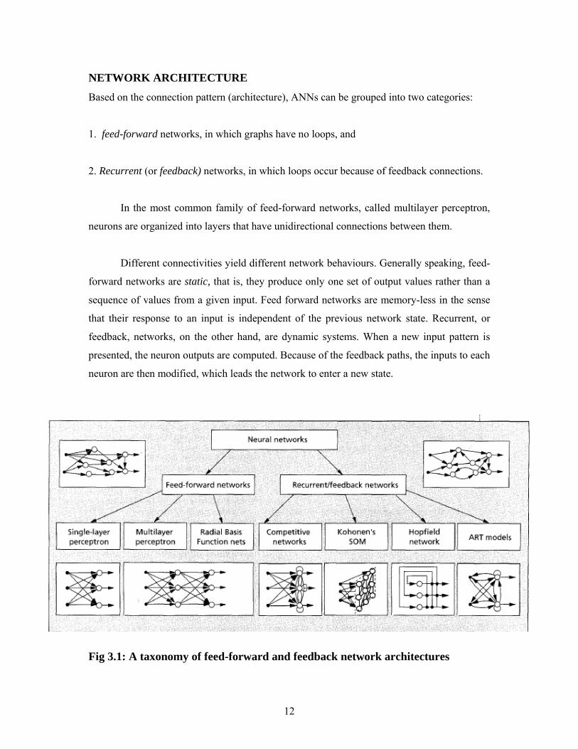
NETWORK ARCHITECTURE

Based on the connection pattern (architecture), ANNs can be grouped into two categories:

1. feed-forward networks, in which graphs have no loops, and

2. Recurrent (or feedback) networks, in which loops occur because of feedback connections.

In the most common family of feed-forward networks, called multilayer perceptron,

neurons are organized into layers that have unidirectional connections between them.

Different connectivities yield different network behaviours. Generally speaking, feed-

forward networks are static, that is, they produce only one set of output values rather than a

sequence of values from a given input. Feed forward networks are memory-less in the sense

that their response to an input is independent of the previous network state. Recurrent, or

feedback, networks, on the other hand, are dynamic systems. When a new input pattern is

presented, the neuron outputs are computed. Because of the feedback paths, the inputs to each

neuron are then modified, which leads the network to enter a new state.

Fig 3.1: A taxonomy of feed-forward and feedback network architectures

13

MULTILAYER PERCEPTRONS

MLPs consist of a number of neurons (or perceptrons) that have inputs and generate

an output using nonlinearity. Neurons in a MLP can be categorized into input neurons, output

neurons and neurons that are neither of the two – so called hidden neurons. An MLP network

is grouped in layers of neurons, i.e. input layer, output layer and hidden layers of neurons that

can be seen as groups of parallel processing units. Each neuron of a layer is connected with

all neurons of the following layer. These connections are directed (from the input to the

output layer) and have weights assigned to. The operation of a MLP can be divided into two

phases:

1. The training phase: Here the MLP is trained for its specific purpose using learning

algorithms (e.g. Back propagation training).

2. The retrieve phase: The previously trained MLPs are used to generate outputs.

Fig 3.2: A structure of MLP

14

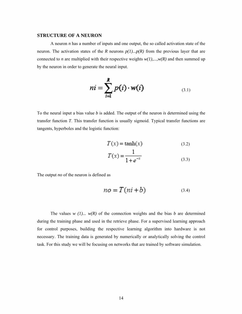
STRUCTURE OF A NEURON

A neuron n has a number of inputs and one output, the so called activation state of the

neuron. The activation states of the R neurons p(1)...p(R) from the previous layer that are

connected to n are multiplied with their respective weights w(1),...,w(R) and then summed up

by the neuron in order to generate the neural input.

(3.1)

To the neural input a bias value b is added. The output of the neuron is determined using the

transfer function T. This transfer function is usually sigmoid. Typical transfer functions are

tangents, hyperboles and the logistic function:

(3.2)

(3.3)

The output no of the neuron is defined as

(3.4)

The values w (1)... w(R) of the connection weights and the bias b are determined

during the training phase and used in the retrieve phase. For a supervised learning approach

for control purposes, building the respective learning algorithm into hardware is not

necessary. The training data is generated by numerically or analytically solving the control

task. For this study we will be focusing on networks that are trained by software simulation.

15

Chapter 4

BACK PROPAGATION ALGORITHM LEARNING

BPA ALGORITHM

FLOW CHART

DATA FLOW DESIGN

16

LEARNING

The ability to learn is a fundamental trait of intelligence. Although a precise definition

of learning is difficult to formulate, a learning process in the ANN context can be viewed as

the problem of updating network architecture and connection weights so that a network can

efficiently perform a specific task. The network usually must learn the connection weights

from available training patterns. Performance is improved over time by iteratively updating

the weights in the network. ANNs' ability to automatically learn from examples makes them

attractive and exciting. Instead of following a set of rules specified by human experts, ANNs

appear to learn underlying rules (like input-output relationships) from the given collection of

representative examples. This is one of the major advantages of neural networks over

traditional expert systems.

To understand or design a learning process, you must first have a model of the

environment in which a neural network operates, that is, you must know what information is

available to the network. We refer to this model as a learning paradigm. Second, you must

understand how network weights are updated, that is, which learning rules govern the

updating process.

A learning algorithm refers to a procedure in which learning rules are used for

adjusting the weights. There are three main learning paradigms: supervised, unsupervised,

and hybrid. In supervised learning, or learning with a “teacher,” the network is provided with

a correct answer (output) for every input pattern. Weights are determined to allow the

network to produce answers as close as possible to the known correct answers.

Reinforcement learning is a variant of supervised learning in which the network is provided

with only a critique on the correctness of network outputs, not the correct answers

themselves. In contrast, unsupervised learning, or learning without a teacher, does not require

a correct answer associated with each input pattern in the training data set. It explores the

underlying structure in the data, or correlations between patterns in the data, and organizes

patterns into categories from these correlations. Hybrid learning combines supervised and

unsupervised learning.

17

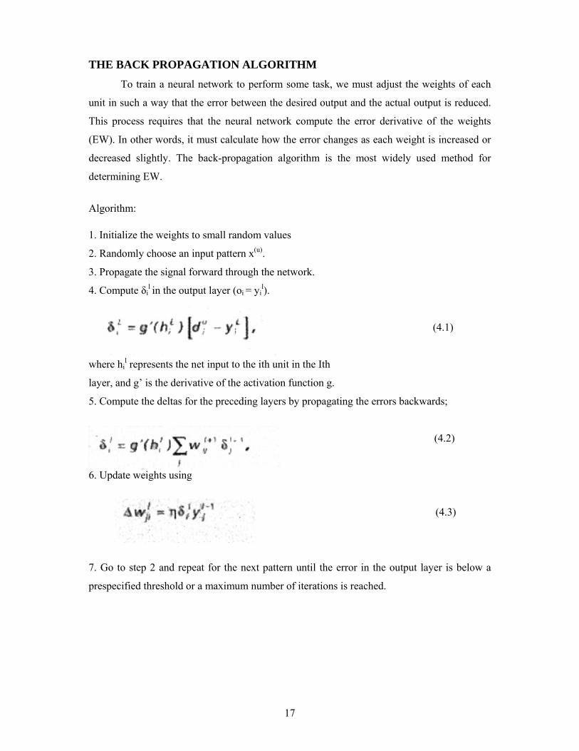
THE BACK PROPAGATION ALGORITHM

To train a neural network to perform some task, we must adjust the weights of each

unit in such a way that the error between the desired output and the actual output is reduced.

This process requires that the neural network compute the error derivative of the weights

(EW). In other words, it must calculate how the error changes as each weight is increased or

decreased slightly. The back-propagation algorithm is the most widely used method for

determining EW.

Algorithm: 1. Initialize the weights to small random values

2. Randomly choose an input pattern x(u).

3. Propagate the signal forward through the network.

4. Compute δil in the output layer (oi = yi

l).

(4.1)

where hil represents the net input to the ith unit in the Ith

layer, and g’ is the derivative of the activation function g.

5. Compute the deltas for the preceding layers by propagating the errors backwards;

(4.2)

6. Update weights using

(4.3)

7. Go to step 2 and repeat for the next pattern until the error in the output layer is below a

prespecified threshold or a maximum number of iterations is reached.

18

FLOW CHART: Yes No Yes No No

No Yes

Compute cycle error E

Get pattern X and feed forward

Initialize weights W for all neurons

Get desired using the equation

Adjust weights for output layer using

F (w, x, d)

START

Adjust weights for hidden layer using

F(w, x, d)

E = 0 More

hidden layers?

More patterns?

E < Emax?

STOP

19

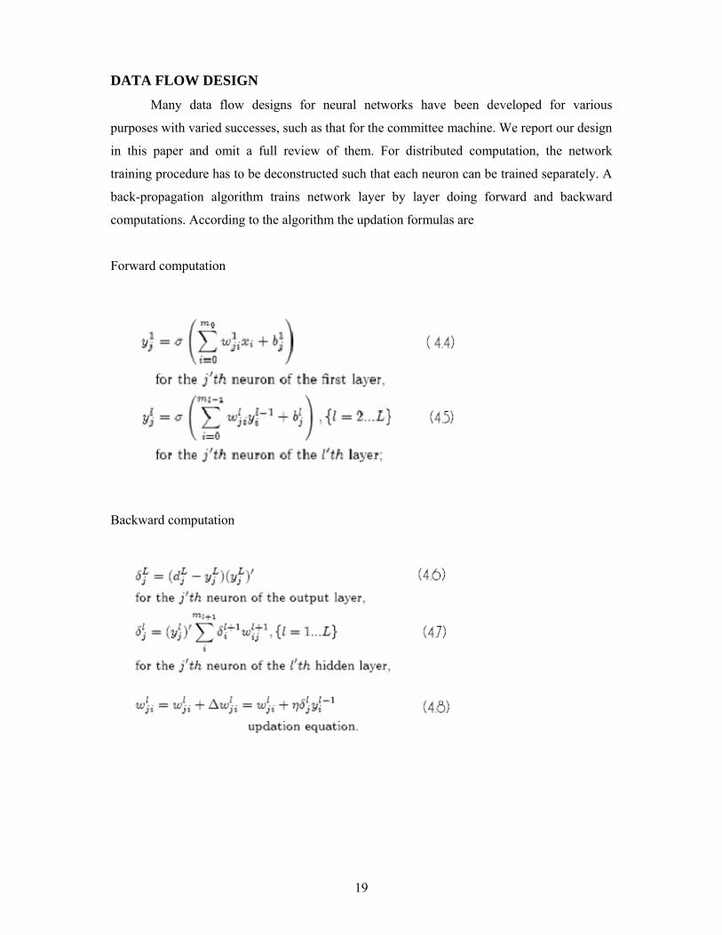
DATA FLOW DESIGN

Many data flow designs for neural networks have been developed for various

purposes with varied successes, such as that for the committee machine. We report our design

in this paper and omit a full review of them. For distributed computation, the network

training procedure has to be deconstructed such that each neuron can be trained separately. A

back-propagation algorithm trains network layer by layer doing forward and backward

computations. According to the algorithm the updation formulas are

Forward computation

Backward computation

20

In the above equations w denotes the weight between two neurons. d is the desired

response. x is the input. y denotes the neuron’s output. σ is the active function. η is a tunable

learning rate. l denotes the number of layer, where 1 denotes the first hidden layer and L is

the output layer. i or j denote the number of neuron in each layer. So, ylj is the output of the

j’th neuron in the l’th hidden layer, wlji is the weight between the j’th neuron in the l’th layer

and the I’th neuron in the (l − 1)’th layer. Blj is the j’th neuron’s bias. dl

j is the desired

response of the j’th neuron in the l’th layer. δlj is the j’th neuron’s delta value for weight

correction. m0 is the number of neurons in input layer, ml−1 is the number of neurons in the (l

− 1)’th layer . All neurons use these equations to improve their weights. Each neuron uses the

outputs of all neurons in the next precedent layer as inputs. We will isolate each neuron with

all its weights, inputs, desired response, and output. This allows us to implement the BP

algorithm on distribute parallel machine.

21

Chapter 5

CHALLENGING PROBLEMS PATTERN RECOGNITION

CLUSTERING

PREDICTION/FORECASTING

OPTIMIZATION

CONTENT ADDRESSABLE MEMORY

FUNCTION APPROXIMATION

22

CHALLENGING PROBLEMS

INTRODUCTION

Let us consider the following problems of interest to computer scientists and

engineers.

PATTERN CLASSIFICATION

The task of pattern classification is to assign an input pattern (like a speech waveform

or handwritten symbol) represented by a feature vector to one of many prespecified classes.

Well-known applications include character recognition, speech recognition, EEG waveform

classification, blood cell classification, and printed circuit board inspection.

CLUSTERING& CATEGORIZATION

In clustering, also known as unsupervised pattern classification, there are no training

data with known class labels. A clustering algorithm explores the similarity between the

patterns and places similar patterns in a cluster. Well-known clustering applications include

data mining, data compression, and exploratory data analysis.

PREDICTION& FORECASTING

Given a set of n samples {y(t1), y(t2) y(t,,)} in a time sequence, t, t2, t,,, the task is to

predict the sample y(t1) at some future time Prediction/forecasting has a significant impact on

decision-making in business, science, and engineering. Stock market prediction and weather

forecasting are typical applications of prediction/forecasting techniques.

OPTIMIZATION

A wide variety of problems in mathematics, statistics, engineering, science, medicine,

and economics can be posed as optimization problems. The goal of an optimization algorithm

is to find a solution satisfying a set of constraints such that an objective function is

maximized or minimized. The Travelling Salesman Problem (TSP), an NP- complete

problem, is a classic example.

23

CONTENT ADDRESSABLE MEMORY

In the von Neumann model of computation, an entry in memory is accessed only

through its address, which is independent of the content in the memory. Moreover, if a small

error is made in calculating the address, a completely different item can be retrieved.

Associative memory or content-addressable memory, as the name implies, can be accessed by

their content. The content in the memory can be recalled even by a partial input or distorted

content. Associative memory is extremely desirable in building multimedia information

databases.

FUNCTION APPROXIMATION

Suppose a set of n labelled training patterns (input-output pairs),{(x1,y1),(x2,y2),...,

(x,y,,)}, have been generated from an unknown function i(x) (subject to noise). The task of

function approximation is to find an estimate, say u^, of the unknown function u. Various

engineering and scientific modelling problems require function approximation. Since our

project is corresponding to the function approximation problem, let us look into this problem

thoroughly by the application of the non-linear model of ADAPTIVE SYSTEM namely

ARTIFICIAL NEURAL NETWORKS.

ANNs apply the principle of function approximation by example, meaning that they

learn a function by looking at examples of this function. One of the simplest examples is an

ANN learning the XOR function, but it could just as easily be learning to determine the

language of a text, or whether there is a tumour visible in an X-ray image.

If an ANN is to be able to learn a problem, it must be defined as a function with a set

of input and output variables supported by examples of how this function should work. A

problem like the XOR function is already defined as a function with two binary input

variables and a binary output variable, and with the examples which are defined by the results

of four different input patterns. However, there are more complicated problems which can be

more difficult to define as functions. The input variables to the problem of finding a tumour

in an X-ray image could be the pixel values of the image, but they could also be some values

extracted from the image. The output could then either be a binary value or a floating point

value representing the probability of a tumour in the image. In ANNs this floating-point

value would normally be between 0 and 1, inclusive.

24

Chapter 6 CHANNEL EUALIZATION INTRODUCTION

NEED FOR EQUALIZATION

CLASSIFICATION OF EQUALIZER

NEURAL NETWORK EQUALIZER

25

INTRODUCTION

First we will understand the reasons that distort the pulses that we transmit over a

communication channel. Then we go to different equalizer structures that were developed

over the decades. The primary being linear transversal equalizer. Then we will observe the

drawbacks in the linear equalizers and why we go for nonlinear structures. Then we

concentrate on the need for decision feedback in an equalizer.

NEED FOR EQUALIZATION

INTERSYMBOL INTERFERENCE (ISI)

Ideally, the impulse response of a linear transmission medium is defined by

)()( τδ −= tAth (6.1)

where t denotes continuous time,

)(th designates the impulse response,

A is an amplitude scaling factor,

)(tδ is the Dirac delta function

τ denotes the propagation delay incurred in the

course of transmitting the signal over the channel.

Equivalently, in frequency domain the above equation can be written as

)exp()( ωτω jAjH −= (6.2)

Where )( ωjH is the frequency response of the transmission media. In practice,

it is impossible for any physical channel to satisfy the stringent requirements embodied in

equations (1) and (2). The best we can do is to approximate equation (2) over a band of

frequencies representing the essential spectral content of the transmitted signal, which makes

the channel ‘dispersive’ [1]. This channel impairment gives rise to ‘Inter-symbol

Interference’. - A smearing of the successive pulses into one another with the result that they

are no longer distinguishable.

26

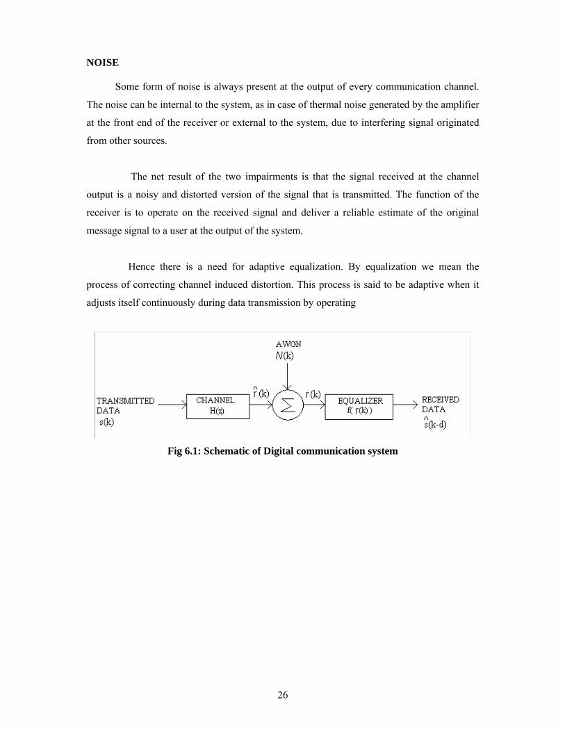
NOISE Some form of noise is always present at the output of every communication channel.

The noise can be internal to the system, as in case of thermal noise generated by the amplifier

at the front end of the receiver or external to the system, due to interfering signal originated

from other sources.

The net result of the two impairments is that the signal received at the channel

output is a noisy and distorted version of the signal that is transmitted. The function of the

receiver is to operate on the received signal and deliver a reliable estimate of the original

message signal to a user at the output of the system.

Hence there is a need for adaptive equalization. By equalization we mean the

process of correcting channel induced distortion. This process is said to be adaptive when it

adjusts itself continuously during data transmission by operating

Fig 6.1: Schematic of Digital communication system

27

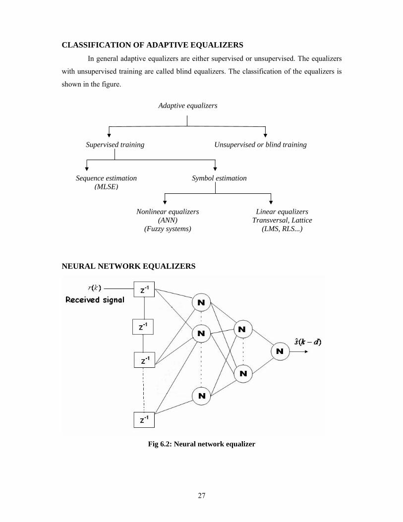
CLASSIFICATION OF ADAPTIVE EQUALIZERS

In general adaptive equalizers are either supervised or unsupervised. The equalizers

with unsupervised training are called blind equalizers. The classification of the equalizers is

shown in the figure.

NEURAL NETWORK EQUALIZERS

Fig 6.2: Neural network equalizer

Supervised training Unsupervised or blind training

Sequence estimation (MLSE)

Adaptive equalizers

Symbol estimation

Nonlinear equalizers(ANN)

(Fuzzy systems)

Linear equalizers Transversal, Lattice

(LMS, RLS...)

28

Back-propagation algorithm is used to train the neural network. The algorithm may

be stated as follows.

Firstly, the correction )()( nynw ijji ∗∗=Δ δη .

Where η is the learning rate parameter

)(njδ is the local gradient

)(nyi is the input signal of neuron j.

Second, the local gradient )(njδ depends on whether neuron j is an input node or a

hidden node:

If neuron j is an output node, )(njδ equals the product of the derivative ))(( nv jjϕ′

and the error signal )(ne j , both of which are associated with neuron j.

If neuron j is a hidden node, )(njδ equals the product of the associated derivative

))(( nv jjϕ′ and the weighted sum of the δ s computed for the neurons in the next hidden or

output layer that are connected to neuron j.

The main disadvantage of using neural networks is that their convergence is slower

compared to linear filters.

The performance of the equalizer is always better than those of linear equalizer.

But there are some channels for which the negative centers and positive centers are very near

and overlap in many cases due to the presence of additive noise. Such channels are called

overlapping channels. One of the examples of such a channel is

216 4084.08164.04084.0)( −− ++= zzzH . (6.6)

Hence we need a decision feedback equalizer to classify these overlapping

patterns. The advantage of the decision feedback equalizer is that ISI is eliminated without

enhancement of noise by using past decisions to subtract out a portion of ISI in addition to

the normal feed forward filter.

29

Chapter 7 FIXED STRUCTURE ANN STRUCTURE OF ANN

RESULTS

30

FIXED STRUCTURE ANN

First we start the project by assuming a fixed structure for the ANN for our

convenience. The structure is given by:

This ANN has 4 layers in total they include the input layer having 9 nodes, the output

layer having 1 node, and the two hidden layers each having 4,3 nodes respectively. This

means our structure can be defined in short as 9,4,3,1 structure. The main advantage of

assuming a structure is to reduce considerably the number of variable parameters of the

ANN.

The various variable parameters of an ANN include:

No. of layers

No. of neurons in each layer

Activation function

Learning factor

Use of batch & sequential mode

So by choosing a fixed structure the other variable parameters get fixed except activation

function which can be varied according to our convenience.

The reason for choosing 9,4,3,1 as the structure is that this structure is universally

regarded as one of the best structure for convergence.

The results for the above structure for various functions and for various activation

function are given in the pages to follow.

31

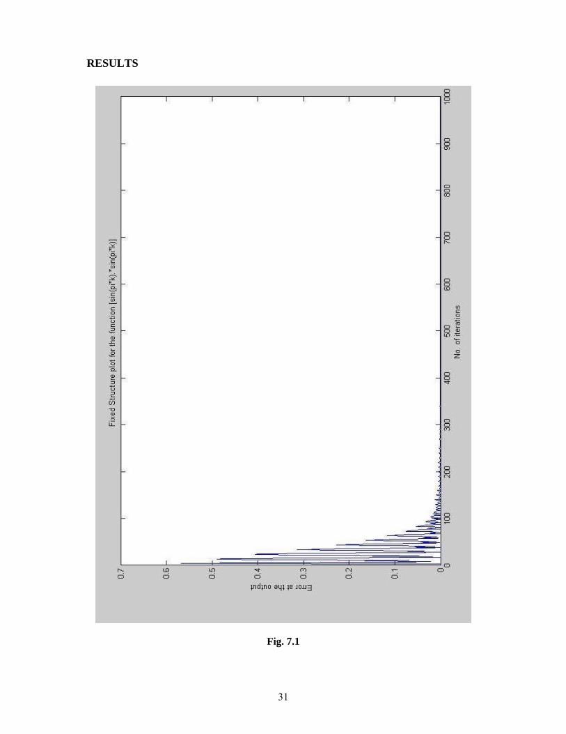
RESULTS

Fig. 7.1

32

Fig. 7.2

33

Fig. 7.3

34

Fig. 7.4

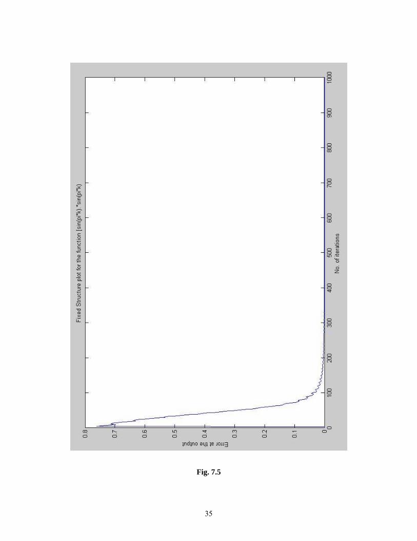
35

Fig. 7.5

36

Chapter 8

GENERALIZED STRUCTURE ANN STRUCTURE

RESULTS

37

STRUCTURE

As said in the chapter above the various variable parameters in the ANN

include:

The various variable parameters of an ANN include:

No. of layers

No. of neurons in each layer

Activation function

Learning factor

Use of batch & sequential mode

The function that we have approximated is a simple square function. The results of

convergence plots for various structures of ANN i.e. for various no. of layers, for various no.

of neurons in each layer, various values of learning rate are obtained and the conclusion for

the optimum no. of layers, for the structure of the no. of neurons in each layer and for the

optimum value of learning rate are deduced.

Here the comparisons are given in terms of groups of three having the same number

of hidden layers and the same number of neurons in each layer for three different values of

the learning factor. The first three graphs correspond to the results of the structure having one

hidden layer, which in turn is having two neurons at three different learning rates. These

learning rates are 0.075, 0.1, 0 .5

The results for the generalized model are shown in the pages to follow.

38

RESULTS

Fig. 8.1

39

Fig. 8.2

40

Fig. 8.3

41

Fig. 8.4

42

Fig. 8.5

43

Fig. 8.6

44

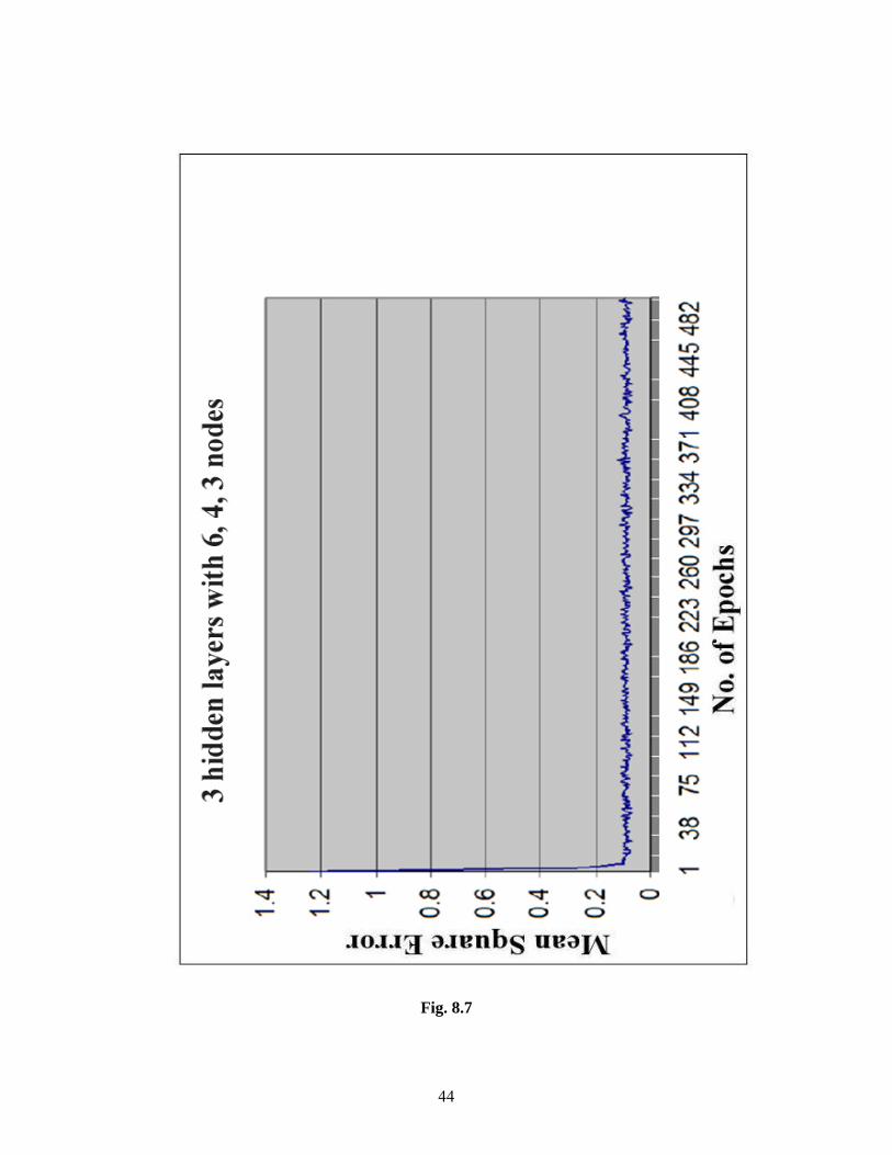
Fig. 8.7

45

Fig. 8.8

46

Fig. 8.9

47

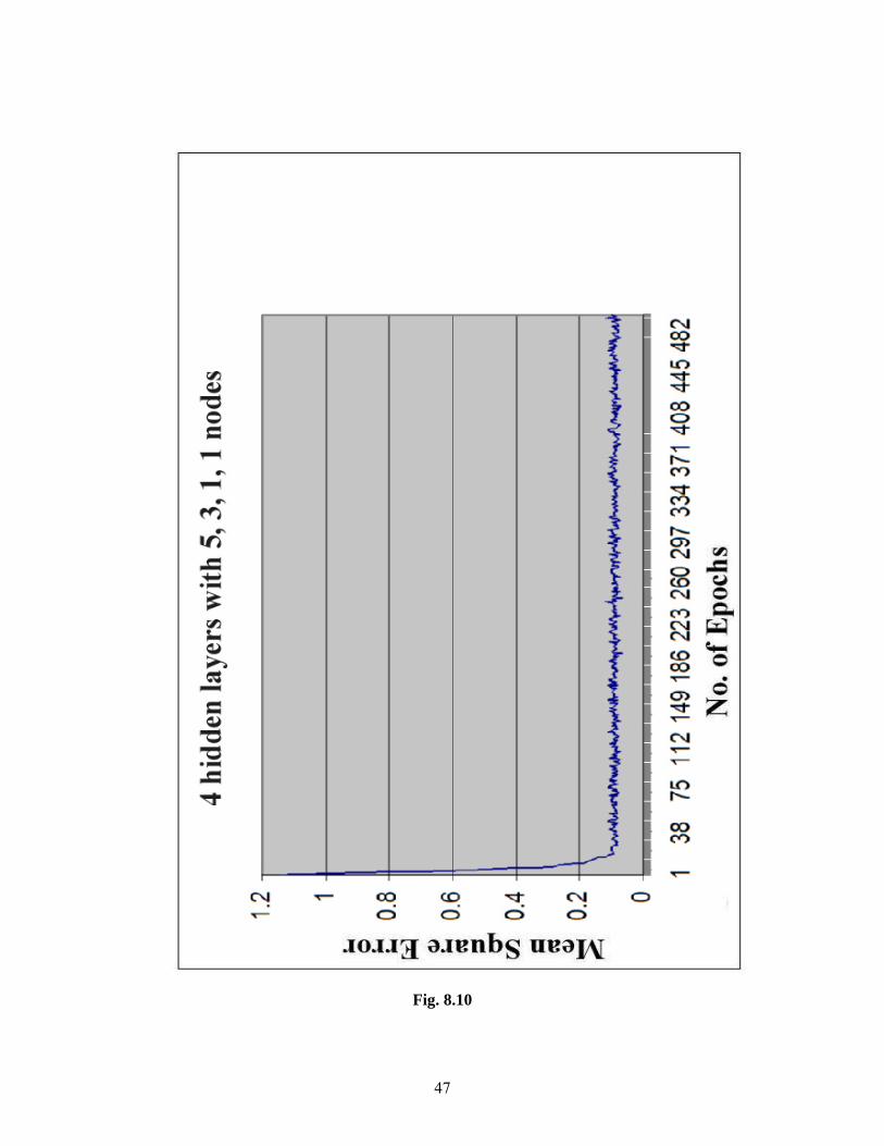
Fig. 8.10

48

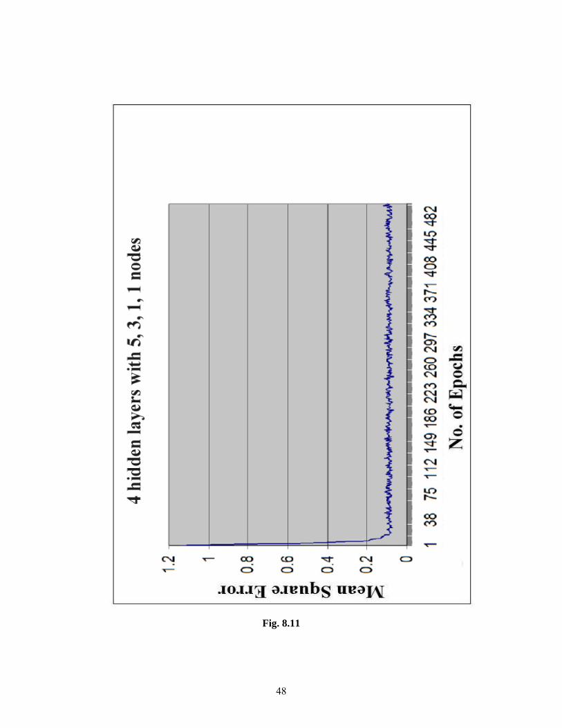
Fig. 8.11

49

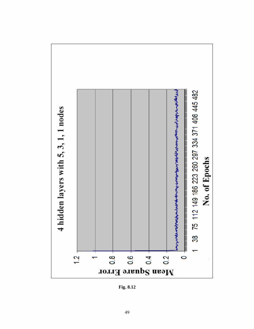
Fig. 8.12

50

Fig. 8.13

51

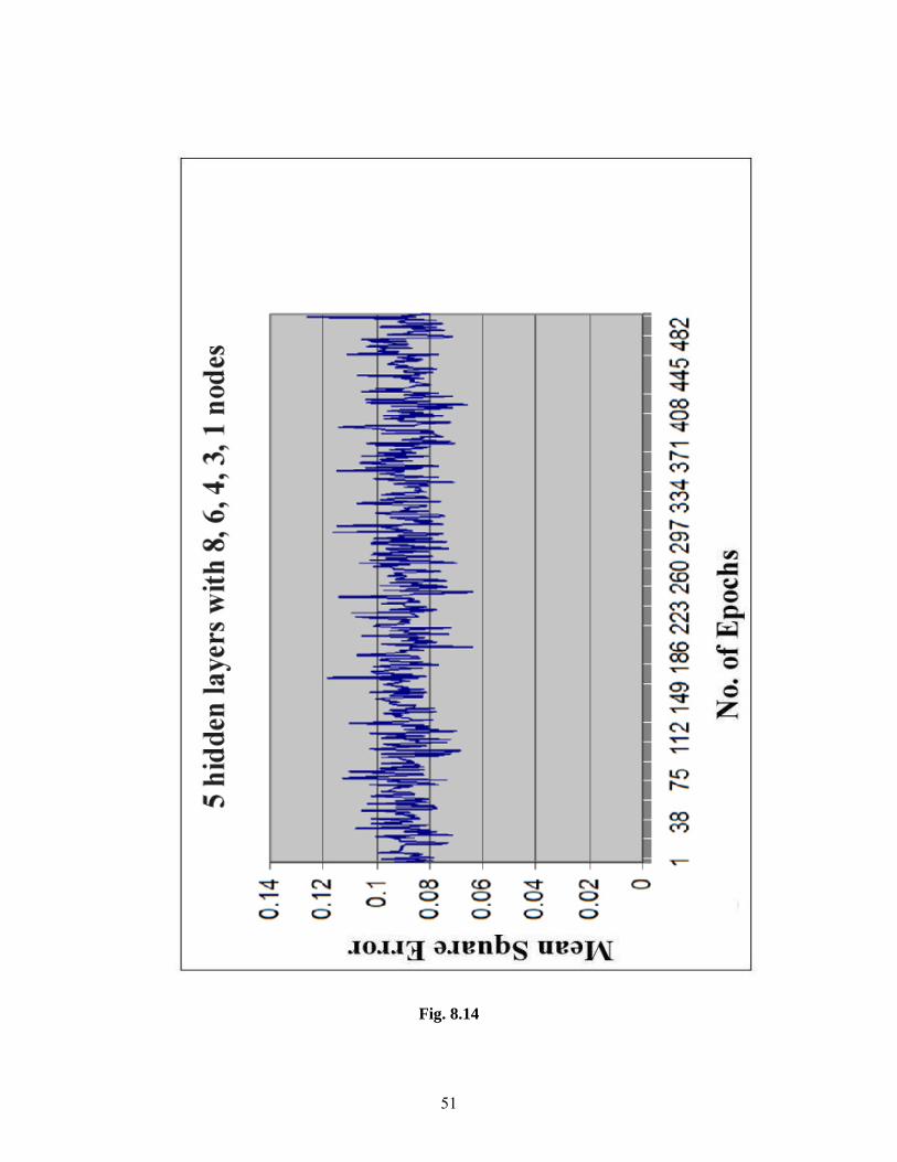
Fig. 8.14

52

Fig. 8.15

53

Fig. 8.16

54

Fig. 8.17

55

Fig. 8.18

56

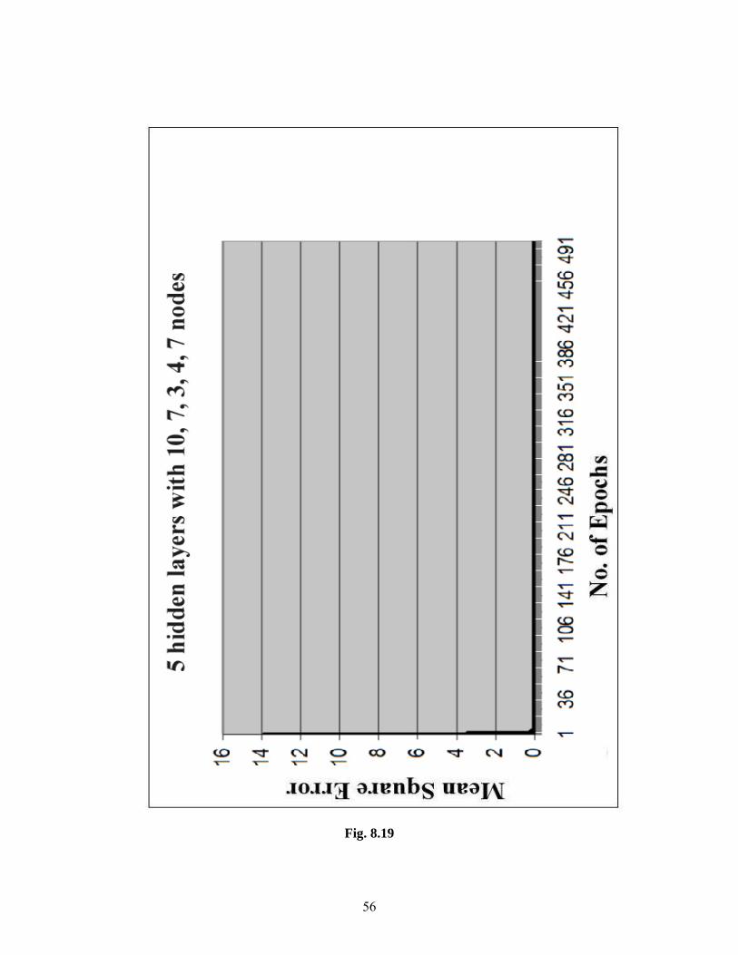
Fig. 8.19

57

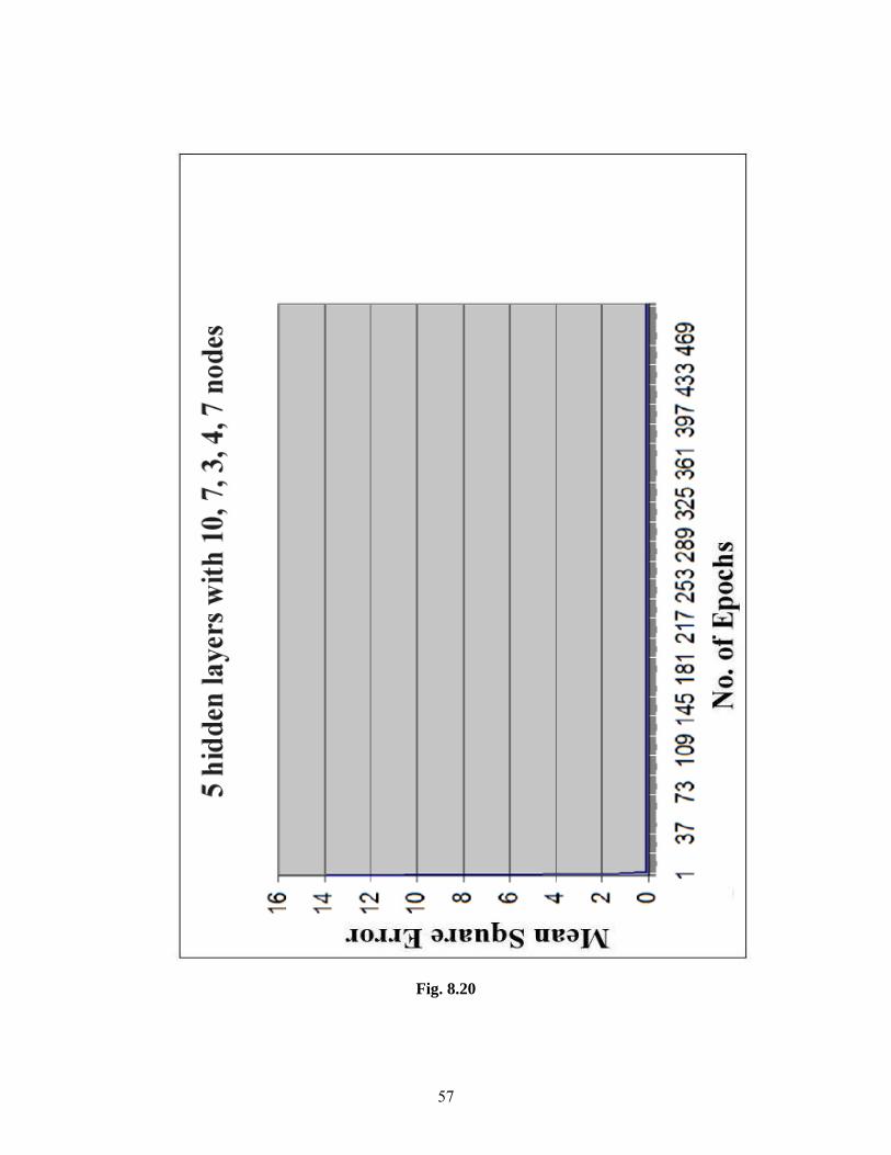
Fig. 8.20

58

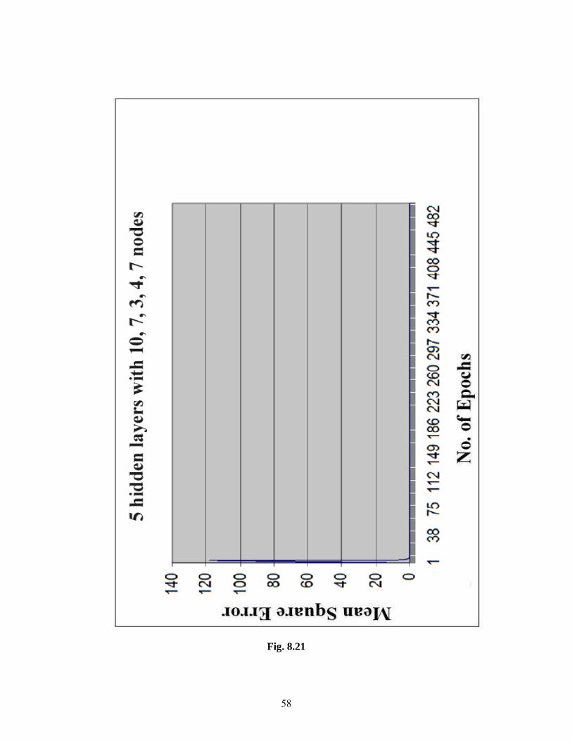
Fig. 8.21

59

Chapter 9

CONCLUSION

60

CONCLUSION

From the above graphs we came to the conclusions regarding the parameters for obtaining the

optimum structure for ANN.

The optimum number of layers including the hidden layers.

Structure for the number of neurons in each hidden layer.

Optimum value for the learning rate.

The difference between the batch& sequential mode.

The graphs are drawn between the number of iterations as the independent variable

and the mean squared error as the dependent variable. From Fig 8.1 it can be seen that the

mean square error starts at 1.6 and gradually reduces to 0.07 at the end of 500 epochs. Thus

we can say that the weights of the ANN model has got trained, and will give the output of the

function approximated for any input with an error up to 0.25

From Fig 8.1- Fig 8.12 it can be seen that the mean square error starts from around a

reasonable value to a minimum of about 0.07 hence these are good examples of training. But

our quest for a best trained ANN structure is not over.

From Fig 8.13- 8.15 show that for a structure like five hidden layers with 8, 6,4,3,1

neurons in each hidden layer have a poor quality of convergence. Here the term convergence

means that the graph between the number of epochs versus the mean square error value must

be smooth. But in the above said graphs the graph is not smooth, even the mean squared error

value just before the 500th epoch is equal to the mean squared error value at the starting of

the program. Therefore we conclude that the structures having a large number of hidden

layers and having the neuron number in each hidden layer in descending order have a poor

quality of convergence. This may be due to over fitting.

Contrary to the above said phenomenon the Figures 8.16- 8.21 show that for the

structures like 4 hidden layers with 9,6,4,6 neurons in respective layers have a very good

quality of convergence. The mean squared error starts at a very high value and at the end of

500th epoch reaches a very low value (as low as 0.07). Hence we can say that the structures

having a medium number of hidden layers with a specific kind of neurons have good quality

61

convergence. Here good convergence is because of the smoothness of the graphs which could

not be observed in case of Figures 8.13- 8.15

The specific kind of structure of ANN, as we have mentioned above is that the

minimum number of neurons are present in the middle hidden layer and it increases on both

sides of this layer. For example if there are four hidden layers, the minimum number of

neurons are present in either of the second or the third hidden layer (9, 6, 4, 6).

Thus we have found out the optimum structure for the ANN model for function

approximation leaving the learning factor parameter untouched. The comparison for getting

the optimal value of the learning rate is given by the graphs in each group. From the graphs it

can be seen that there is no much difference between them as the learning rats is increased.

Hence we choose an optimal value for the learning rate as 0.1.

Hence it can be seen that the Fig 8.17 represents the best structure for function

approximation at the above said learning rate.

62

REFERENCES

1. Jose D. Martin-Guerrero - Luis Gomez-Chova – Gustavo Camps-Valls - Antonio

Serrano-Lopez - Joan Vila-Frances - Javier Calpe-Maravilla - Emilio Soria-Olivas,

“Journal of Electrical Engineering”, Vol. 55, No. 5-6, 2004, 156-160.

2. Lipo Wang, Jagath C. Rajapakse, Kunihiko Fukushima, Soo-Young Lee, and Xm

Yao, “Proceedings of the 9th International Conference on Neural Information

Processing (ICONIP'02)”, Vol. 1, 2002.

3. Graham C. Goodwin - Centre for Complex Dynamic Systems and Control, Day 5:

Lecture 4, 17th September 2004.

4. Cheng- Yuan Liou and Yen-Ting Kuo, “Dept. of Computer Science and Information

Engineering, National Taiwan University Supported by National Science Council

under Project NSC 90-2213-E-002-092”

5. Cangelosi, A., S. Nolfi, and D. Parisi, “Cell division and migration in a 'genotype' for

neural networks, Network- Computation in Neural Systems”, 1994, 5:497-515.

6. Xin Yao, Senior Member, IEEE “Invited Paper Proceedings of the IEEE”, September

1999, Vol. 87, No. 9.

7. S. C. Ng, S. H. Leung and A. Luk, IEEE 0-7803-5471-0/99, 1999.

8. HE Zhen-ya, “The Adaptive Signal Processing”. Bei Jing: Science Press, 2002:1-54. 9. DARFA Neural Network Study, A FCEA Int’l Press, Fairfax, Va., 1998.

10. Haykin Simon, “Neural Networks: A Comprehensive Foundation”, New Jersey:

Macmillan Publishing Company, 1994.

11. PROAKIS, J. G., “Digital Communications”, New York: McGraw-Hill, 3rd edition

1995.

12. Jain Ani1 K. - Michigan State University, Mao Jianchang, K.M. Mohiuddin – IBM

Admaden Research Center, “IEEE journal”, 0018-9162/96 March 96.

13. Veen, Arthur H, “Dataflow Machine Architecture. ACM Computing Surveys”, Vol.

18, No. 4, Dec. 1986, pp. 365-396.

14. X. Yao, “Evolution of connectionist networks,” in Preprints Int. Symp. AI, Reasoning

& Creativity, Queensland, Australia, Griffith Univ., 1991, pp. 49–52.

function approximation using back...

Documents